Abstract
Inappropriate soil management accelerates soil erosion and thus poses a serious threat to food security and biodiversity. Due to poor data availability and fragmented terrain, the landscape pattern of garden erosion in tropical Xishuangbanna is not clear. In this study, by integrating multi-source satellite imagery, field investigation and visual interpretation, we realized high-resolution mapping of gardens and soil conservation measures at the landscape scale. The Chinese Soil Loss Equation (CSLE) model was then performed to estimate the garden erosion rates and to identify critical erosion-prone areas; the landscape pattern of soil erosion was further discussed. Results showed the following: (1) For the three major plantations, teas have the largest degree of fragmentation and orchards suffer the highest soil erosion rate, while rubbers show the largest patch area, aggregation degree and soil erosion ratio. (2) The average garden erosion rate is 1595.08 t·km−2a−1, resulting in an annual soil loss of 9.73 × 10⁶ t. Soil erosion is more susceptible to elevation and vegetation cover rather than the slope gradient. Meanwhile, irreversible erosion rates only occur in gardens with fraction vegetation coverage (FVC) lower than 30%, and they contribute 68.19% of total soil loss with the smallest land portion, indicating that new plantations are suffering serious erosion problems. (3) Garden patches with high erosion intensity grades and aggregation indexes should be recognized as priorities for centralized treatment. For elevations near 1900 m and lowlands (<950 m), the decrease in the fractal dimension index of erosion-prone areas indicates that patches are more regular and aggregated, suggesting a more optimistic conservation situation.
1. Introduction
Soil erosion refers to the process of detachment and removal of soil by exogenous forces; it is the main cause of land degradation and as a consequence leads to reduced productive capacity of agriculture and terrestrial ecosystems, posing a severe threat to the achievement of the Sustainable Development Goals [1,2,3]. Soil erosion depends on both anthropogenic factors and natural conditions. It is commonly accepted that serious soil erosion generally does not take place under natural conditions, as the vegetation cover forms a sound protection for soil against detachment, which reduces its vulnerability to soil erosion [4,5]. However, human interventions, such as land use change, deforestation, overgrazing, slope reclamation and intensive tillage, accelerate the soil erosion process dramatically, with current rate orders of magnitude higher than the natural soil formation rate [6,7,8].
For decades, increasing attention has been paid to study the soil erosion of cultivated land (mainly grains) worldwide, as it is the primary source of soil loss and sediment [6,9]; about 80% of agricultural land worldwide suffers from moderate to severe erosion [10]. However, garden land, as an indispensable form of agriculture land, suffers serious soil erosion problems and has been largely ignored thus far, especially at the landscape scale [11]. Garden lands include orchards, tea gardens, mulberry gardens, rubber plantations and other gardens such as those for planting grapes, coffee, cocoa, pepper, flowers and medicinal herbs [12,13]. The tropical Xishuangbanna (XSBN) region has the most concentrated garden plantations in China, motivated by economic interests, traditional croplands and biodiverse natural forests, that are continuously being reclaimed as garden plantations, mostly for monoculture rubbers and teas [14,15].
Compared with natural forests, garden plantations under rain-fed agriculture are especially susceptible to soil erosion and inappropriate soil management for several reasons. Firstly, a vegetation canopy has a great impact on rainfall interception and buffering, but the long-term vegetation cover of monoculture garden plantations is less stable, resulting in reduced rainfall interception ability [16,17,18]. Meanwhile, mostly planted in transition zones onto steep highlands, the poor water-holding capacity of soil makes it vulnerable to climate change and human activities [19]. In addition, gardens usually lack land levelling and soil conservation measures like terraces but are intensively managed for high production and high yield; fertilizers, herbicides and weeding are commonly used to keep the soil surface bare and exposed [20,21], especially for orchards (Figure 1). The rapid expansion of gardens and intensive farming activities undoubtedly brings serious soil erosion and land degradation problems and poses a profound impact on habitats’ fragmentation, ecosystem service losses, water shortages and poor carbon sequestration capacities [2,9,22]. To assess the environmental impacts of erosion and find strategies to deal with them, quantitative information on the erosion characteristics of garden land is crucial.
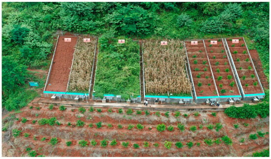
Figure 1.
Views of typical garden land (citrus orchards, plots 5–7) showing evidence of high soil erosion rates compared to bare soil (plot 1), cropland (plot 2 and plot 4) and shrub (plot 3) in our field experiments.
A wide variety of approaches, such as empirical models and physically based models, as well as radioisotopic and physicochemical background indicators [23,24,25], have been employed to quantify garden erosion rates at different temporal and spatial scales. Specifically, these are the Universal Soil Loss Equation (USLE) [26], the revised RUSLE [27], the Water Erosion Prediction Project (WEPP) [28], the sediment delivery distributed (SEDD) model [29] and the 137Cs method [30]. For regions like Mediterranean areas, tropical regions and the Loess Plateau, high soil erosion rates have been observed in the different kinds of land of garden plantations involving vineyards [31], citrus [32], olive orchards [33], apricots [4], tea [30] and rubber [34]. In terms of surface runoff and sediment loss control, previous studies have also confirmed the efficiency of major conservation measures in reducing garden erosion [35,36,37], including contour tillage [38], grass cover [39], straw mulching [40], intercropping [18], hedgerows [41] and terracing [42]. To date, satellite data have provided significant information for mapping, monitoring and predicting runoff and soil erosion, and mainly follow two main lines of research [43,44,45]: the monitoring of signals, which describes variations of earth surface characteristics [46,47,48], and the improvement of modelling methods with signals of hydrological or geomorphological variables relevant to the erosion processes [24,49,50].
However, most soil erosion models are established based on the scale of plot size, hill slope and catchment, with certain applicable conditions and scopes. When applied to regional or landscape scales, the establishment conditions of the model, the characteristics of the applicable objects and the requirements for input variables or parameters must be simplified accordingly, and the reliability of the results is often questioned. In addition, due to the similar spectrum between garden plantations and other vegetation and to poor remote-sensing data availability in cloudy and rainy mountainous regions, many limitations still exist in identifying gardens and soil conservation measures at large scales using single-sensor data, as most land use/cover (LULC) products cannot provide the distribution information of complex fragmented garden lands, as well as the conservation measures, including the leading LULC products, such as ESA_WorldCover, Dynamic_World from Google and ESRI Land_Cover with a 10 m resolution. At present, the contradiction between the low resolution of available data in fragmented mountainous areas and the high resolution required to study the runoff–erosion process brings huge difficulties and challenges to the quantification of soil erosion [51]. Specifically, little research has been carried out on garden erosion on the landscape scale in tropical Xishuangbanna with complex erosion environments.
In recent years, the use of landscape pattern metrics and multi-source remote sensing imagery to describe soil erosion landscape patterns and their inter-relationships has gained a lot of attention, but few related studies of garden erosion in tropical regions have been reported so far, despite the fact land area transformed to rubber, tea and fruit production is booming, and the distribution of gardens has obvious vertical zonal characteristics. The reasons behind this are the poor data availability and quality, since in tropical mountainous areas, the fragmented terrain, cloudy and rainy weather (low image availability), complex planting system of gardens, unobservable soil conservation measures, limitations of soil erosion models and similar spectral features between gardens and vegetation all lead to uncertainty in high-precision garden land mapping. To effectively control soil loss from garden plantations, it is of great significance to quantify soil erosion rates, identify critical erosion hotspots using multi-source satellite imagery and a well-proved model and implement targeted soil management interventions at the landscape scale.
Take the garden plantations of XSBN as the research object; the aims of this study, therefore, were to (a) obtain high-precision distribution information of gardens and soil conservation measures; (b) quantitatively estimate the soil erosion modulus according to the CSLE model, and combine the landscape metrics to reveal the vertical landscape pattern characteristics of garden erosion; (c) identify critical soil-erosion-prone areas by analyzing garden erosion variations and regional differences, and provide scientific basis for the determination of priority areas of human interventions in the region.
2. Materials and Methods
2.1. Study Area
Xishuangbanna Dai Autonomous prefecture is situated in the extreme south of Yunnan province, southwest China, and lies between 21°08′N–22°36′N and 99°56′E–101°50′E. The prefecture covers an area of about 19,200 km2, and shares borders with Laos and Myanmar (Figure 2). Altitude varies from 477 to 2429 m above the sea level. With the Hengduan Mountains running north–south, high mountains and deep valleys characterize the prefecture and about 95% of the region is mountainous. The Lancang River (upper reaches of the Mekong River) runs through the center of XSBN from north to south. XSBN sits on the northern edge of the tropics south of the Tropic of Cancer, and is one of the only two places in China that are considered to have a tropical monsoon climate [52]. Specifically, the uplifted Himalayas forms a barrier preventing cold continental air masses of a subtropical origin in winter, and enables the penetration of warm–wet tropical air masses from the Indian Ocean in summer, resulting in a rainy season lasting from May to October and a dry season from November to April [53,54]. The average annual temperature is 15.1–21.7 °C, and the mean annual rainfall ranges from 1200 to 2500 mm, with average annual precipitation of about 1500 mm, of which nearly 90% occurs in the rainy season, showing an uneven distribution in time and space [55]. Laterite soils developed from siliceous rocks (600–1000 m), the lateritic red soil (above 1000 m) and the limestone soils are the dominant soil types in XSBN [56], and the major soil groups (FAO/UNESCO classifications) are Acrisols, Alisols, Cambisols and Anthrosols, characterized by being rich in clay and formed under conditions of high precipitation and temperature. The combination of geography and climate creates a vast territory with diverse and unique natural resources, making the region with the highest level of biodiversity in China. During the past decades, the landscape in XSBN has changed dramatically due to the conversion from tropical rainforests to rubbers, especially for the lowlands, which have already been fully utilized [57].
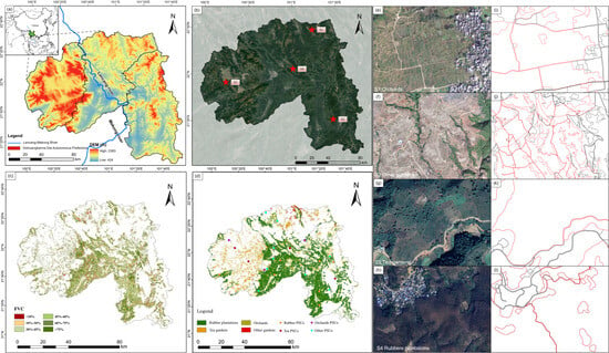
Figure 2.
(a) Map of XSBN showing its location, elevation and counties; (b) S1–S4 are orchards, other gardens, tea gardens and rubber plantations, and high-resolution remote sensing images of XSBN. (c) Fraction vegetation coverage of gardens in XSBN in 2020; (d) distribution of gardens in XSBN in 2020 and Primary Sample Units with measured erosion rates for validation in the National Soil Erosion Survey in China; (e−l) are high-resolution satellite images of GF–7, Beijing–2 and Sentinel–2 and corresponding retrieved garden polygons (red ones).
2.2. Data Sources
Critical data concerning garden erosion quantification at the landscape scale were obtained as follows: daily erosive rainfall (≥12 mm) data from 143 weather stations in a recent-30-year download from the National Meteorological Data Sharing Service System (http://data.cma.cn, accessed on 20 June 2022) were employed to compute the rainfall erosivity. Soil profiles and soil-type data (347 series, 18 groups, 42 soil sub-groups), including soil organic matter, texture, permeability and structure, collected from the Second National Soil Survey in China, were used to acquire soil erodibility using the USLE nomograph. ALOS DEM data (https://search.asf.alaska.edu/, accessed on 1 July 2022) of 12.5 m were used to calculate terrain factors using the maximum downhill slope methods (proposed by Hickey) and the segment slope length equation (proposed by Foster). The multi-source remote sensing data include the time series Sentinel−2A/B, Landsat 8 OLI images (a total of 340 images, accessed on 1 June 2022, to retrieve vegetation index) and two high-resolution satellites in China, including GF−7 (0.8 m) images and Beijing−2 (resolution of 0.65 m) from the Third National Land Resources Survey, which were prepared to derive a garden land use map and soil conservation distribution map at the regional scale in XSBN. The land use map of gardens, therefore, consists of two parts; one is automatic image classification [58] (we proposed a classification method combining multi-source phenology characteristics and a random forest algorithm for rubber identification with the highest accuracy in this region in our previous work), and the other is visual interpretation of sub-meter-resolution images. All these data were resampled to a 10 m spatial resolution (requirements for input variables in CSLE) before incorporated as input layers in the CSLE model for a further analysis. Primary Sample Units (PSUs) with measured garden erosion rates allocated in XSBN from the National Soil Erosion Survey were used for validation of our estimation (Figure 3).
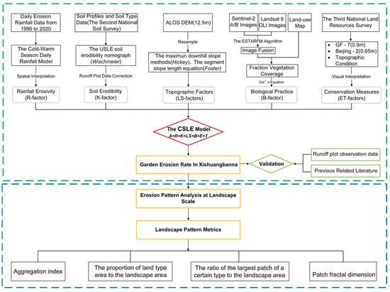
Figure 3.
Schematic flowchart of the methodology employed in this study.
2.3. Methodology
2.3.1. The CSLE Model
Since the 1980s, by modifying parameters of the Universal Soil Loss Equation (USLE) to target areas, many scholars have proposed different regional soil loss prediction models. In 2002, Liu et al. developed the Chinese Soil Loss Equation (CSLE) based on measured data from a unit plot and numerous plots modified to it [59,60]. As the official model of the Ministry of Water Resources of China (MWRC) for water erosion assessment, the major differences of CSLE compared to USLE are modifications made for steep slope conditions and a complex soil conservation measure system. CSLE is a statistical relationship model that correlates the soil erosion rate and the affecting factors, which can be modified according to the local conditions and has been widely verified and applied. The greatest advantage of CSLE is that it is more in line with the actual topographical conditions and the soil conservation measure system in China, and the two factors of cover management and support practices (C, P) in USLE were modified into three factors of biological measures (B), engineering measures (E) and tillage measures (T). Five dimensionless factors of slope length, slope gradient, biological measure, engineering measure and tillage measure are used to modify the soil loss determined by the dimensional rainfall erosivity and soil erodibility in the model. The CSLE formula is expressed as follows [61]:
where A is the soil erosion modulus with a unit of t/(hm2·a); R describes the erosive force of rainfall and runoff, which is referred to as rainfall erosivity, MJ·mm/(hm2·h·a); K represents soil’s susceptibility to be detached and transported by the actions of raindrops and runoff, t·hm2·h/(MJ·hm2·mm); L is the slope length factor and S is the slope steepness factor; B is the biological measure factor; E is the engineering measure factor; T is the factor of tillage measures; B-, E-, T-factors have a dimensionless range of 0–1 and the smaller the value is, the better the soil conservation effect of a certain measure is.
Among the 7 input indicators in CSLE, soil conservation measures largely control the magnitude and variability of soil erosion, and are the ones that are rarely considered in large-scale soil erosion modelling, since it is difficult to estimate in fragmented mountainous areas. The specific calculation methods of R-, K-, L- and S-factors were described in detail in our previous work [59,60] and related literature [62,63,64,65,66]. Here, we focus on the biggest obstacle to quantify soil erosion for complex terrain areas at the landscape scale, which is the implication of soil conservation measures. Due to the influence of cloudy and rainy weather and low image availability, for a long time, low–medium spatial resolution remote sensing images have had great limitations in tropical areas with complex terrain, fragmented land and mixed vegetation, and it is difficult to capture scattered garden land patch distribution, not to mention soil conservation measures. Therefore, we proposed an approach that combines phenology characteristics and a random forest algorithm using the GEE cloud platform, and achieved sound identification of rubber (the most dominant garden land type in XSBN) at the regional scale [58]. To acquire a continuous accurate distribution of all garden types in XSBN, we used the commercial satellite data (with sub-meter resolutions) provided in the Third National Land Survey as well as field investigation to perform visual interpretation for the whole prefecture. We also detected information such as the engineering measure type and area percentage of engineering measures adopted in all gardens.
The B-factor refers to the ratio of soil loss under a certain vegetation coverage condition to soil loss under the same condition in cleared fallow land, reflecting the relative magnitude of soil loss under vegetation coverage compared to soil loss without it. Since soil erosion has a significant negative exponential relationship with vegetation cover, and the role of vegetation cover in controlling soil erosion is well recognized. In this study, the ESTARFM Algorithm [67] was used to fuse time series Sentinel−2A/B and Landsat8 images, to construct functional relationships between adjacent months and establish multi-source time series continuous fraction vegetation coverage (FVC) data with a resolution of 10 m monthly. And with the aid of the GEE cloud computing platform, the pixel binary model was used to divide different planting crops to effectively estimate the vegetation coverage [54]. The basic idea is assuming that the surface of a pixel is composed of a vegetation coverage part and non-vegetation part, the weight of each surface part is determined by the proportion of the respective area to the pixel and the percentage of the land surface covered by vegetation in the pixel is defined as FVC; the B-factor was then calculated using a formula proposed by Cai [68]. Similar to the C-factor in the USLE, B values are weighted average soil loss ratios (Bi), which change as vegetation cover changes during the process of plant growth. The B value then represents the average of Bi values, each weighted by the portion of rainfall erosivity during the same time period. The calculation formulas for affecting factors are listed as follows:
where R is the average annual rainfall erosivity (MJ∙mm∙ha−1∙h−1∙a−1), k represents the 12 months in a year, Rk is the average rainfall erosivity in the k-th month (MJ∙mm∙ha−1∙h−1∙a−1), N refers to the time series from 1990 to 2020, the term α is a value of 0.3937 for the warm season and 0.3101 for the cold season, Pi,j,k is the actual erosive rainfall (≥12 mm) of the j-th day in the k-th month in the i-th year, m is the number of days with erosive rainfall in the corresponding month. WRk is the ratio of average rainfall erosivity in the k-th month to the average annual rainfall erosivity, which reflects the seasonal distribution of rainfall erosivity.
where K is soil erodibility, N1 (particle size: 0.002–0.1 mm) is the percent of silt (0.002–0.05 mm) plus very fine sand (0.05–0.1 mm), N2 (<0.002 mm) is the clay fraction, (100 − N2) (0.002–2 mm) represents all soil fractions other than clay, OM is the soil organic matter content (%), S is the soil structure code and P is the soil permeability code.
where Li is the slope length factor of the i-th pixel, λout and λin are the pixel exit and entrance slope lengths and m is the slope length exponent depending on the slope.
where NDVImax refers to the regional maximum NDVI; NDVIveg is the NDVI value of the pure vegetation pixels; NDVIsoil is the NDVI value of the pure bare soil pixels; Bi is the B-factor of the i-th month. The relationship between the FVC and B value was compiled using Equation (12).
The P-factor in the USLE is described as the engineering measure factor (E) and tillage measure factor (T) in the CSLE. Engineering measures refer to the measures adopted by changing micro terrain conditions to intercept surface runoff, increase soil rainfall infiltration or improve agricultural production conditions, such as the sloping terrace, level terrace, check dam, fruit tree pit, intercepting drain, diversion canal, etc. Tillage measures are usually taken with cultivated equipment, such as those to enhance soil resistance to erosion, and reduce erosion by increasing crop cover and soil infiltration. For most garden lands, the T value equals to 1 as no tillage measure applies.
A terrace is the most common soil conservation measure in South China. According to field investigation, the most dominant soil conservation measures in XSBN are interval terraces, slope terraces, horizontal terraces and inward (reverse) sloping bench terraces, and the effect in controlling soil erosion of those measures has been well studied with plot experiments. The E-factor represents the ratio of soil loss by adopting certain engineering measures to soil loss without engineering measures under the same conditions. Based on a field survey, with reference to corresponding E values from runoff plot experiments [69,70] by local experts, we decoded the engineering measures by visual interpretation with high-resolution images, and the observed E value of the corresponding typical engineering measure was summarized (Table 1); the E value was assigned to 1 for areas without protection. Garden erosion quantification results were then obtained by putting each index layer with a raster multiply operation.

Table 1.
Descriptions, interpretation symbols and E values of typical engineering measures in gardens.
2.3.2. Landscape Pattern Metrics
The landscape pattern metrics describe the complexity of patch types and arrangements, including features such as patch shape, size, number and spatial combination. A single index cannot comprehensively present the characteristics of a landscape ecological pattern [71,72]. Soil erosion is a multiscale, non-linear spatial geo-ecological process, which includes the in situ stripping of soil materials, transport and deposition along the earth surface [72]. Landscape elements act on the whole process of soil erosion, and their spatial configuration also poses a significant impact on soil erosion. Therefore, the quantitative method of landscape metrics can be introduced to the field of soil erosion to make up for the insufficient study in large scales [73,74,75,76].
To analyze and describe the landscape pattern characteristics of garden erosion, on the basis of referring to the existing research results, this study selects the landscape pattern metrics with ecological significance: the patch fractal dimension, the ratio index of the largest patch to the landscape area, the proportion of land-type area to the landscape area and the aggregation index. With reference to previous research [75] and actual terrain conditions, the study area was divided into different elevation zones and Fragstats4.2 software was applied to discuss the vertical landscape characteristics of soil erosion intensity. The calculation formula and landscape pattern index metrics used are as follows:
- Patch fractal dimension (D):
- b.
- Ratio of the largest patch of a certain type to the landscape area (LPI):
- c.
- Proportion of land-type area to the landscape area (PLAND):
- d.
- Aggregation index (AI, %):
3. Results
3.1. Spatial Distribution of Garden Plantations in XSBN
According to the land use map, XSBN had a total garden land area of 6121.88 km2 in 2020, of which rubber accounted for 4526.74 km2, teas occupied 862.78 km2, orchards took up 629.79 km2 and other gardens took up 102.57 km2, with percentages of 73.94%, 14.09%, 10.29% and 1.68%, respectively. Rubber dominates the prefecture in terms of land use and economy at low–mid elevation, as do teas at high elevations. Still, a large amount of high-elevation lands is being converted for rubbers and teas due to actual profits far exceeding other agricultural types such as rice, fruit, vegetables and livestock. For the three administrative units, Jinghong and Mengla share a similar distribution of terrain, and the low–mid-elevation areas in the southern parts of both counties are mainly planted with monoculture rubber. The major difference is Jinghong owns more tea gardens at higher altitudes compared to Mengla, which has more nature reserves and forest. As Menghai is at a much higher altitude where teas grow well and there are few lowland areas that are suited for rubber, tea gardens are the dominant garden land type in Menghai, followed by immature rubber plantations, orchards and other gardens that are generally planted fragmentedly in the landscape.
For the three major garden types, tea plantations are mostly found above 900 m, with the largest fragmentation degree and smallest average patch size, followed by orchards, which are only one-sixth in size compared to that of rubbers (Table 2). The minimum patch area is similar, while the maximum patch areas are quite different from each other, and the patch shape for rubbers and tea gardens is much more complex than orchards.

Table 2.
Patch distribution of each garden type in XSBN.
Garden plantation distribution in XSBN shows a decreasing trend with the increase in the elevation and slope gradient, and is more sensitive to altitude than slope. By analyzing the distribution in different altitude ranges and slope intervals, about 82% of the gardens are concentrated on slopes of 5–30°, with a mean slope gradient of 19.4° for all gardens and the largest proportion at slopes of 10–15°, showing a wide range of planted areas at all slopes (Figure 4a). There are also significant differences in the distribution of gardens across altitude zones; nearly 90% of the prefecture’s gardens are located in areas of elevation below 1200 m, with 43.14% of the gardens concentrated in the 700–950 m zone, much higher than in other elevation classes. Specifically, rubbers are mainly planted in the 700–950-m-elevation zone, and tea plantations are widely distributed in the 700–1700-m-elevation zone (Figure 4b).

Figure 4.
Distribution of gardens at different (a) slope gradient and (b) elevation zones in XSBN.
3.2. Spatial Pattern of Garden-Erosion-Affecting Factors
The R-factor (rainfall erosivity) in XSBN shows a decreasing trend both from south to north and from east to west, and ranges from 3674.28 to 8399.39 MJ·mm/(hm2·h·a), with an average value of 5470.10 MJ·mm/(hm2·h·a) (Figure 5a). The K-factor (soil erodibility) in Figure 5b varies from 0.002 to 0.009 t·hm-2·h/(MJ·mm·hm2), with a mean value of 0.0061 t·hm2·h/(MJ·mm·hm2). High K values are mostly found in inter-mountain basins and valley areas adjacent to the Lancang-Mekong River. The value range of LS-factors (Figure 5c) is 0–63.53, with an average value of 10.92, and the highest values are found in the transition zone from basin areas to a mountain front. The B-factor (vegetation) in Figure 5d varies from 0 to 1, with an average value of 0.1217. Overall, tea gardens, orchards and other gardens are higher in B values compared to rubber plantations, due to the relative lower vegetation coverage.
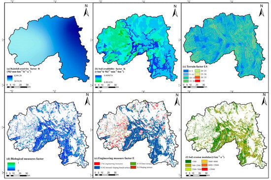
Figure 5.
Spatial distribution maps of soil-erosion-affecting factors and soil erosion modulus estimated using the CSLE model. (a) Rainfall erosivity; (b) Soil erodibility; (c) Topographic factors; (d) Vegetation cover factor; (e) Engineering factor; (f) Soil erosion modulus.
We also quantified the role of typical soil conservation measures in XSBN based on reported field measurements (ISBT, ST, IT) from local experts. As can be seen in Figure 5e, about 81.65% of the gardens in XSBN are treated with certain engineering measures, and the distribution area is ISBT > ST > IT. ISBT (E = 0.343) occupies an area of 4311.82 km², and is widely distributed in areas with slopes less than 25°, with its area gradually decreasing when the slope is greater than 25° (Figure 6). ST (E = 0.4) takes up an area of 527.32 km², mainly covering slopes of 20°–25°, while IT (E = 0.114) shows the best efficiency in soil conservation but has the smallest area (163.05 km2), and is mainly distributed on slopes with a gradient of less than 20°. Nevertheless, a garden land area of about 1123.93 km² is still under no protection in the prefecture.
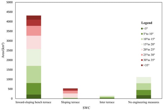
Figure 6.
Typical soil conservation measures implemented for gardens at different slope gradient classes in XSBN.
3.3. Soil Erosion of Garden Plantations in XSBN
As can be seen from the garden erosion modulus map (Figure 5f), lower soil erosion rates are mainly found in the central part of XSBN planted with rubber; high values are dispersedly distributed in steep slopes planted with teas and fruits. The mean garden erosion modulus is 1595.08 t·km−2a−1, which is about three times the soil loss tolerance (T) of 500 t·km−2a−1 in this region, and the average annual soil loss is 9.73 × 10⁶ t. Average soil erosion rates of a rubber plantation, tea plantation, orchard and other gardens are 1564.75 t·km−2a−1, 1590.22 t·km−2a−1, 1827.54 t·km−2a−1 and 1548.90 t·km−2a−1, respectively. Gardens affected by soil erosion (above tolerant) in XSBN make up 3009.45 km2, accounting for 49.34% of the total land area. Most gardens (85.50%) fall within low erosion intensity grades, and only account for about 30% of the soil loss. At the landscape scale, both the distribution and soil erosion rate of gardens decrease as the altitude increases. Gardens with erosion intensity grades above moderate erosion (6.73% of the total land area) contribute more than half of the total soil loss (Table 3). Apparently, garden erosion has high heterogeneity in this region and critical-erosion-prone areas exist in certain locations. By referring to the SL190–2007: Standard for Classification and Gradation of Soil Erosion (Table 3), gardens in XSBN were further divided into six soil erosion intensity grades with different soil erosion rate ranges.

Table 3.
Soil erosion intensity grades of garden lands in XSBN.
The difference in soil erosion can be attributed to the following reasons: rubbers are planted in a wide range of XSBN, and the vegetation coverage is generally high, which has a great effect on intercepting and buffering rainfalls, resulting in a relative lower erosion rate among gardens. But due to the large planted area and dominant rainfall forces, rubber contributes the largest portions of the eroded area, erosion ratio and total soil loss. For tea plantations widely distributed in high-altitude areas in Menghai in the west, they also face serious soil erosion problems due to the steep terrain, despite the low rainfall erosivity. For newly planted gardens that lack engineering conservation measures and vegetation cover, soil erosion is especially not negligible. Most orchards often undergo weeding to keep the ground bare to increase yields, leaving soils directly exposed to heavy rainstorms; thus, orchards show the most serious erosion rates among gardens, but because of the small planted area, they only account for 11.77% of total soil loss (Table 4).

Table 4.
Soil erosion status of different garden plantations in XSBN.
3.4. Validation of the CSLE Estimated Erosion Rates
Different data resolutions or quality brings different results within the same area. In this study, validation was carried out by using measured soil loss data in the National Soil Erosion in China, a total of 24 Primary Sample Units of gardens in XSBN (Table 5). The land uses of those plots were garden land with slopes’ gradient ranging from 5° to 25°. The determination coefficient R2 and root mean square error (RMSE) between the measured and estimated erosion results were applied for validation. Our study showed that the R2 and RMSE of CSLE were 0.92 and 6.85 t·ha−1·a−1, respectively. About 75.0% of plots had absolute errors within 5 t·ha−1·a−1 (Figure 7), indicating the high-precision performance of the CSLE in XSBN, which also conformed the data accuracy for erosion modeling and conservation measures.

Table 5.
Primary Sample Units of gardens in XSBN in the National Soil Erosion Survey (NSES) in China for validation.
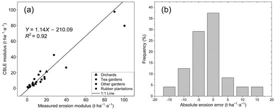
Figure 7.
(a) Validation of estimated soil erosion rates using CSLE model; (b) the absolute error distribution frequency for estimated erosion results.
It should be noted that there is no linear positive correlation between erosion intensity grades and slope gradient (Figure 8a). In terms of the composition of soil erosion grades at different slope gradient zones, except for tolerant grades, the proportion of all erosion grades increases as slope increases. High erosion intensity grades (above moderate erosion) mainly occur at slopes between 10 and 30 ° (Figure 8c). Meanwhile, garden erosion intensity grades are linearly negatively correlated with vegetation coverage (Figure 8b). Almost all the garden plantations that show high soil erosion rates are characterized by FVC values lower than 30%, especially those gardens with FVC less than 10%, which have an average irreversible erosion rate of about 8000 t·km−2a−1, as well as the largest deviation. For gardens with FVC values under 30%, the erosion contribution is about 68.19% of the total soil loss, while garden land of the remaining vegetation coverage classes only contributes 31.81% of the erosion amount (Figure 8d). Given that low vegetation coverage is the necessary condition for high soil erosion rates of gardens in XSBN, soil erosion is far more sensitive to the influence of vegetation coverage than to the slope gradient, and areas with low vegetation coverage on steep slopes, especially those lower than 30%, are undoubtedly critical target area for soil erosion control efforts.
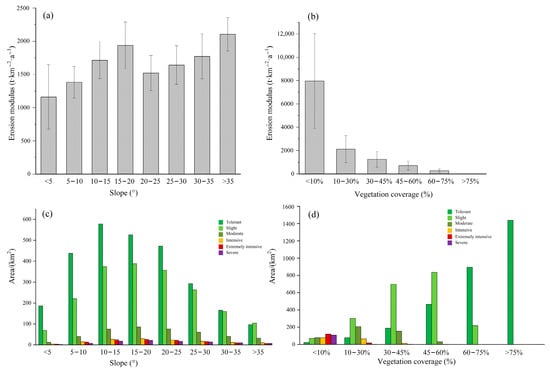
Figure 8.
Garden erosion modulus of different slope gradients (a) and vegetation coverage classes (b); area distribution of garden erosion intensity grades for different slope gradient (c,d) vegetation coverage in XSBN.
3.5. Landscape Pattern of Garden Erosion Intensity
Existing studies rarely analyze the characteristics of agricultural land erosion from the landscape scale, so we employed four metrics with landscape ecological significance to study the differentiation characteristics of garden soil erosion patches, especially in the vertical dimension, to better reveal the law of soil erosion in a complex mountain environment.
On the landscape scale, the patch fractal dimension (D) reflects the shape complexity of garden patches with different erosion intensity levels. As can be clearly seen, garden patches with soil erosion intensity grades of slight, moderate and intensive show higher average D values, indicating that garden patches of these three types of erosion are more complex in shape (Figure 9a). However, low D values are mostly found in garden patches without erosion (tolerant), as well as those with the most serious erosion grades, indicating that their shapes are simpler and more regular; to some extent, human activities have different degrees of intervention in the soil erosion process. Those severely eroded gardens with simpler shapes at lower altitudes undoubtedly signal for better soil conservation measures. Except for tolerant grades, as soil productivity is sustainable, in the remaining five grades, four of them show the characteristics of more complex patch shapes as the altitude increases, indicating that human activities pose much more intervention to garden erosion in lowlands compared to the higher regions, and natural factors are more influential than human factors at higher elevations. Undoubtedly, D value trends for different soil erosion intensities vary considerably at different altitudes, since the degree of human intervention on rubbers, teas, orchards and other plantations is also quite different. The coefficient of variation (CV) is the absolute value that reflects the degree of dispersion of the data. To quantify the magnitude of D value variation in the vertical dimension, the CV of D values for different soil erosion intensities in the elevation zone was calculated and ordered: intensive (1.44%) > severe (1.11%) > tolerant (1.05%) > extremely intensive (1.00%) > moderate (0.96%) > slight (0.81%). Apparently, with the increase in altitude, intensive erosion shows a large fluctuation, while slight erosion exhibits the best stability in each elevation zone, which is mainly due to the fact that most of the garden patches are suffering from soil erosion of this intensity grade.
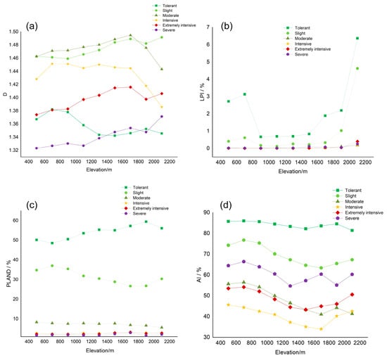
Figure 9.
Landscape metric curves of (a) D, (b) LPI, (c) PLAND and (d) AI for garden erosion intensity in XSBN.
LPI refers to the proportion of the largest land patch to landscape area. In both horizontal and vertical dimensions, LPI values for gardens in XSBN generally decrease with increasing erosion intensity grades, except for small fluctuations in a few elevation ranges. However, LPI values fluctuate more in the vertical dimension. Except for tolerant grades, the average LPI curves for the other five grades are stable and with values less than 1 (Figure 9b), indicating that garden patches are scattered and no phenomenon of concentrated contiguous distribution exists. Tolerant and slight erosion have the largest LPI values, indicating that they are the most dominant types in the study area, especially in areas above 1900 m. For low altitudes, only the tolerant grade shows a dominant distribution due to the widespread distribution of rubber fields with high vegetation coverage. In most mid-elevation classes (900–1500 m), garden erosion intensity grades exhibit higher diversity.
The difference from the LPI value is that the PLAND value places more emphasis on the place of a certain soil erosion type in the landscape, rather than describe the structural characteristic of a single patch, but it does show the same average value trend of a decrease as soil erosion intensity increases (Figure 9c). Low erosion intensities show the absolute dominance in land use distribution at all elevation zones. The sum of the PLAND values of each erosion intensity at the same elevation interval on the vertical axis is 1. In general, tolerant and slight erosion show a trade-off relationship. For uplands, the proportion of tolerant erosion is greater, while in low-elevation areas, the erosion ratio of garden land is higher; especially at an altitude near 700 m, the occurrence probability of the unsustainable soil erosion rate in garden land is the highest. Soil erosion intensity has obvious vertical differentiation, and at low altitudes, although the slope is gentler and the vegetation coverage is higher, there is more precipitation and human activities are more intensive. As the altitude increases, the land of forest and grassland increases, the proportion of garden lands continues to decrease, despite slope increases, the impact of human activities decreases and the connectivity of garden patches tends to be less.
For the aggregation index (AI) of patches, all AI values decrease first and then increase as there is an increase in erosion intensity in the horizontal dimension (Figure 9d). However, the degree of patch aggregation shows a more complex law in the vertical dimension, and the garden patches do not show the characteristics of aggregation linearly with the decrease in the erosion intensity level. The mean AI values in descending order are tolerant > slight > severe > extremely intensive > moderate > intensive. In the 700–1300-m-elevation zones, the aggregation degrees of all intensity grades are decreasing, but in the zones above 1300 m, the aggregation degrees of different erosion intensity grades begin to have different peaks and valleys. Although the land area of high erosion intensity levels is small, considering the outstanding contribution to the total soil erosion amount, finding the local peaks of the AI curves means a lot for the decision making regarding priority and order of soil erosion control. For example, the AI curve shows a local peak at the altitude of 1700 m. However, for all types of erosion intensity, the concentration and aggregation of garden plots between 500 and 900 m are much higher; thus, the allocation of soil and water conservation funds for garden plantations at this elevation can be regarded as priorities and directions. Overall, garden erosion in XSBN has higher heterogeneity in the vertical dimension compared to the horizontal dimension.
4. Discussion
At the landscape scale, limited by the availability and quality of satellite data, it is difficult to extract complex soil conservation measures and multiple cropping structures of gardens only using a single method or single-sensor data. We employed the non-homogenous data voting and random forest classification method to identify rubber distribution in XSBN, and combined a field survey, visual interpretation and model calculation to accurately map the distribution of soil conservation measures and garden erosion in XSBN. However, the process is expensive and time-consuming; machine learning algorithms and cloud computing show promising potential in soil erosion modeling, not only in vegetation-related index inversion. This specifically applies to identifying characteristics of the soil surface by different wavelengths, temporal changes of surface states, incision and geometry of possible water pathways on the surface. Whether for thematic information extraction, thematic mapping, dynamic change monitoring or remote sensing database construction, automatic image classification technology is inseparable. In the future, incorporating field surveys and the spectral–spatial information or other features of gardens in different spectral bands to obtain the fine classification of erosion-related ground features is the focus of the next step.
So far, quantitative assessment of garden erosion is rarely reported at the landscape scale, and most quantitative studies focus on the observation scale of runoff plots, land parcels or small watersheds. In this paper, by improving the accuracy and precession of the input parameters of the CSLE model, we achieved a solid estimation compared with existing observations, and the CSLE model was proven to be a suitable approach for estimating soil loss for the mountainous region. It should be noted that the model is developed to predict long-term averages of sheet and rill erosion from a single slope, and erosion types like gully erosion, freeze–thaw erosion and gravitational erosion are not included. Despite the interpretation of aerial imagery allowing the detection of many conservation measures, the role of typical soil conservation measures was quantified based on previous runoff plot observations from local experts in the region, which is especially important for the CSLE model to perform more reliable erosion estimation. According to the field investigation, we found a huge difference in the vegetation coverage extracted by medium–low-resolution satellite imagery generally overestimated the actual situation, especially in the newly cultivated tea gardens and orchards, which are prone to soil erosion. Nevertheless, how to quantify the scale problem of multi-source data in erosion estimation and its impact on the calculation results needs further discussion with more plot experiments.
For fragmented mountainous areas, the ecological effects of garden erosion such as land degradation and rocky desertification are very prominent, yet they are still not being taken seriously. Due to the fragmented distribution and complex natural environment of gardens, factors like land plowing, multiple cropping, intercropping and crop rotation systems pose significant impact on soil erosion; especially the cultivation and planting modes are constantly changing with crop types, climate, spatial location and seasons. In this study, all the garden crops are regarded as a single monoculture structure, but a substantial portion of orchards and tea gardens has been converted from cropland during the adoption of the Grain for Green Project (returns farmland to forest and grass) in China since 2000; they still retain many characteristics of the original cultivated land, which introduces uncertainty in the erosion rate estimation. Meanwhile, whether the extensive conversion of farmland to forests has achieved the expected benefits needs to be further evaluated from different perspectives, especially the impact on the sustainability of biodiversity, carbon sequestration and clean water sources.
5. Conclusions
Landscape-scale soil erosion assessment is the critical method of decision making associated with land resource management and soil conservation planning. In this paper, to gain a clear understanding of soil erosion in garden plantations in XSBN, we combined multi-source remote sensing data, such as GF−7, Beijing−2 and Sentinel−2 A/B, the CSLE model and landscape metrics to quantitatively estimate garden erosion for the first time at the landscape scale in XSBN, and the following findings were obtained:
- (1)
- Garden distribution in XSBN shows obvious vertical zoning differentiation, and is more sensitive to altitude change rather than the slope gradient, showing a decreasing trend as the altitude increases. In total, 90% of the gardens in XSBN are distributed in low-altitude areas below 1200 m, of which more than 40% are concentrated in the 700–950-m-altitude zone, much higher than other altitude zones. Orchards and teas are fragmented and mostly planted on slopes, while rubbers are clustered.
- (2)
- In total, 49.34% of the gardens in XSBN are being eroded at an erosion rate higher than the soil loss tolerance. The average garden erosion rate in XSBN is 1595.08 t·km−2a−1, which is three times the accepted rate to sustain soil productivity, and the annual soil erosion amount is 9.73 × 10⁶ tons. Extreme and severe erosion are mostly found in those garden lands with FVC lower than 30%, which contribute about 68.19% of the total soil loss. For the three major garden types, orchards suffer from the most serious erosion problem with an erosion rate of 1827.54 t·km−2a−1. Gardens with soil erosion intensity higher than the grade of intensive only account for 6.73% of the total garden area, but contribute more than 50% of the total soil loss amount from gardens. Still, a garden land area of about 1123.93 km² is still under no protection in the prefecture.
- (3)
- The spatial analysis of garden erosion intensity demonstrated that heterogeneity in the vertical dimension is much more complex compared to the horizontal dimension. Affected by human activities, garden patches of lowlands (especially near 700 m) are simpler in shape and high in the erosion ratio. Patches of tolerant and slight erosion intensity dominate the landscape, especially in lowlands and areas above 1900 m, showing a high aggregation degree and stability. Meanwhile, garden patches exhibit higher diversity of soil erosion intensity grades in the mid-elevation classes (900–1500 m). The peaks and troughs of landscape metric curves are critical in identifying garden erosion hotspots, for patches that are high in both erosion intensity and aggregation degree can be regarded as priorities of soil erosion control efforts. As the pressure of population and economy growth keeps driving garden plantations onto increasingly steep slopes, soil erosion occurring under a rubber canopy also needs sufficient attention from relevant departments to maintain sustainable development in tropical areas.
Author Contributions
R.T.: Data curation, Formal analysis, Software, Writing; G.C.: Conceptualization, Methodology, Funding, Writing, Editing; B.T.: Supervision, Review; Y.H.: Data curation, Review; X.M.: Investigation, Review; Z.L.: Image and data processing, Validation; J.F.: Date collection, Visualization. All authors have read and agreed to the published version of the manuscript.
Funding
This research is supported by the Basic Research Project of Yunnan Province (Grant No. 202101AU070161) and the Strategic Priority Research Program of Chinese Academy of Sciences (Grant No. XDA26050301-01).
Data Availability Statement
Available upon request.
Acknowledgments
We deeply thank the related organizations for permitting us to use the data and Wen Qinke of Aerospace Information Research Institute, Chinese Academy of Sciences, for her valuable suggestions.
Conflicts of Interest
The authors declare that they have no known competing financial interest or personal relationships that could have appeared to influence the work reported in this paper.
References
- Morgan, R.P.C. Soil Erosion and Conservation; John Wiley & Sons: New York, NY, USA, 2009. [Google Scholar]
- Borrelli, P.; Robinson, D.A.; Fleischer, L.R.; Lugato, E.; Ballabio, C.; Alewell, C.; Meusburger, K.; Modugno, S.; Schutt, B.; Ferro, V.; et al. An assessment of the global impact of 21st century land use change on soil erosion. Nat. Commun. 2017, 8, 13. [Google Scholar] [CrossRef] [PubMed]
- Liu, B.Y.; Yang, Y.; Lu, S.Y. Discriminations on common soil erosion terms and their implications for soil and water conservation. Sci. Soil Water Conserv. 2018, 16, 10–16. (In Chinese) [Google Scholar]
- Keesstra, S.; Pereira, P.; Novara, A.; Brevik, E.C.; Azorin-Molina, C.; Parras-Alcantara, L.; Jordan, A.; Cerda, A. Effects of soil management techniques on soil water erosion in apricot orchards. Sci. Total Environ. 2016, 551, 357–366. [Google Scholar] [CrossRef] [PubMed]
- Duan, J.; Liu, Y.J.; Yang, J.; Tang, C.J.; Shi, Z.H. Role of groundcover management in controlling soil erosion under extreme rainfall in citrus orchards of southern China. J. Hydrol. 2020, 582, 10. [Google Scholar] [CrossRef]
- Wuepper, D.; Borrelli, P.; Finger, R. Countries and the global rate of soil erosion. Nat. Sustain. 2020, 3, 51–55. [Google Scholar] [CrossRef]
- Borrelli, P.; Ballabio, C.; Yang, J.E.; Robinson, D.A.; Panagos, P. GloSEM: High-resolution global estimates of present and future soil displacement in croplands by water erosion. Sci. Data 2022, 9, 9. [Google Scholar] [CrossRef] [PubMed]
- Kemp, D.B.; Sadler, P.M.; Vanacker, V. The human impact on North American erosion, sediment transfer, and storage in a geologic context. Nat. Commun. 2020, 11, 9. [Google Scholar] [CrossRef]
- Pope, I.; Harbor, J.; Zanotti, L.; Shao, G.; Bowen, D.; Burniske, G.R. Cloud Forest Conservation in the Central Highlands of Guatemala Hinges on Soil Conservation and Intensifying Food Production. Prof. Geogr. 2016, 68, 1–13. [Google Scholar] [CrossRef]
- Meliho, M.; Nouira, A.; Benmansour, M.; Boulmane, M.; Khattabi, A.; Mhammdi, N.; Benkdad, A. Assessment of soil erosion rates in a Mediterranean cultivated and uncultivated soils using fallout 137Cs. J. Environ. Radioact. 2019, 208, 10. [Google Scholar] [CrossRef]
- Guo, L.J.; Liu, R.M.; Men, C.; Wang, Q.R.; Miao, Y.X.; Shoaib, M.; Wang, Y.F.; Jiao, L.J.; Zhang, Y. Multiscale spatiotemporal characteristics of landscape patterns, hotspots, and influencing factors for soil erosion. Sci. Total Environ. 2021, 779, 13. [Google Scholar] [CrossRef]
- Sun, H.L. Chinese Encyclopedia of Resource Science; Encyclopedia of China Publishing House: Beijing, China, 2000; pp. 124–156. [Google Scholar]
- The Detailed Rules for the Land Classification of the Third National Land Survey, Ministry of Natural Resources of the People’s Republic of China. Available online: https://www.mnr.gov.cn/ (accessed on 20 June 2022).
- Liu, X.N.; Feng, Z.M.; Jiang, L.G.; Zhang, J.H. Spatial-Temporal Pattern Analysis of Land Use and Land Cover Change in Xishuangbanna. Resour. Sci. 2014, 36, 233–244. (In Chinese) [Google Scholar]
- Chen, H.F.; Yi, Z.F.; Schmidt-Vogt, D.; Ahrends, A.; Beckschafer, P.; Kleinn, C.; Ranjitkar, S.; Xu, J.C. Pushing the Limits: The Pattern and Dynamics of Rubber Monoculture Expansion in Xishuangbanna, SW China. PLoS ONE 2016, 11, 15. [Google Scholar] [CrossRef]
- Zhu, X.I.; Yuan, X.; Lu, E.F.; Yang, B.; Wang, H.F.; Du, Y.Y.; Singh, A.K.; Liu, W.J. Soil splash erosion: An overlooked issue for sustainable rubber plantation in the tropical region of China. Int. Soil Water Conserv. Res. 2023, 11, 30–42. [Google Scholar] [CrossRef]
- Liu, W.J.; Luo, Q.P.; Lu, H.J.; Wu, J.N.; Duan, W.P. The effect of litter layer on controlling surface runoff and erosion in rubber plantations on tropical mountain slopes, SW China. Catena 2017, 149, 167–175. [Google Scholar] [CrossRef]
- Zhu, X.A.; Chen, C.F.; Wu, J.N.; Yang, J.B.; Zhang, W.J.; Zou, X.; Liu, W.J.; Jiang, X.J. Can intercrops improve soil water infiltrability and preferential flow in rubber-based agroforestry system? Soil Tillage Res. 2019, 191, 327–339. [Google Scholar] [CrossRef]
- Wang, S.S.; Sun, B.Y.; Li, C.D.; Li, Z.B.; Ma, B. Runoff and Soil Erosion on Slope Cropland: A Review. J. Resour. Ecol. 2018, 9, 461–470. [Google Scholar]
- Wang, X.X.; Sun, Y.Y.; Hu, Y.; Zhu, C.J. Impact of Weeds on Surface Runoff and Soil Loss in a Navel Orange Orchard. J. Weed Sci. 2019, 37, 23–28. (In Chinese) [Google Scholar]
- Liu, H.X.; Blagodatsky, S.; Giese, M.; Liu, F.; Xu, J.C.; Cadisch, G. Impact of herbicide application on soil erosion and induced carbon loss in a rubber plantation of Southwest China. Catena 2016, 145, 180–192. [Google Scholar] [CrossRef]
- Sarathchandra, C.; Abebe, Y.A.; Worthy, F.R.; Wijerathne, I.L.; Ma, H.X.; Bi, Y.F.; Guo, J.Y.; Chen, H.F.; Yan, Q.S.; Geng, Y.F.; et al. Impact of land use and land cover changes on carbon storage in rubber dominated tropical Xishuangbanna, South West China. Ecosyst. Health Sustain. 2021, 7, 14. [Google Scholar] [CrossRef]
- Igwe, P.U.; Onuigbo, A.A.; Chinedu, O.C.; Ezeaku, I.I.; Muoneke, M.M. Soil erosion: A review of models and applications. Int. J. Adv. Eng. Res. Sci. 2017, 4, 237341. [Google Scholar]
- Borrelli, P.; Alewell, C.; Alvarez, P.; Anache, J.A.A.; Baartman, J.; Ballabio, C.; Bezak, N.; Biddoccu, M.; Cerda, A.; Chalise, D.; et al. Soil erosion modelling: A global review and statistical analysis. Sci. Total Environ. 2021, 780, 18. [Google Scholar] [CrossRef]
- Laflen, J.M.; Flanagan, D.C. The development of US soil erosion prediction and modeling. Int. Soil Water Conserv. Res. 2013, 1, 1–11. [Google Scholar] [CrossRef]
- Alewell, C.; Borrelli, P.; Meusburger, K.; Panagos, P. Using the USLE: Chances, challenges and limitations of soil erosion modelling. Int. Soil Water Conserv. Res. 2019, 7, 203–225. [Google Scholar] [CrossRef]
- Renard, K.G. Predicting Soil Erosion by Water: A Guide to Conservation Planning with the Revised Universal Soil Loss Equation (RUSLE); ARS: Washington, DC, USA, 2013. [Google Scholar]
- Flanagan, D.C.; Gilley, J.E.; Franti, T.G. Water Erosion Prediction Project (WEPP): Development history, model capabilities, and future enhancements. Trans. ASABE 2007, 50, 1603–1612. [Google Scholar] [CrossRef]
- Taguas, E.V.; Moral, C.; Ayuso, J.L.; Perez, R.; Gomez, J.A. Modeling the spatial distribution of water erosion within a Spanish olive orchard microcatchment using the SEDD model. Geomorphology 2011, 133, 47–56. [Google Scholar] [CrossRef]
- Gharibreza, M.; Samani, A.B.; Arabkhedri, M.V.; Zaman, M.; Porto, P.; Kamali, K.; Sobh-Zahedi, S. Investigation of on-site implications of tea plantations on soil erosion in Iran using Cs-137 method and RUSLE. Environ. Earth Sci. 2021, 80, 14. [Google Scholar] [CrossRef]
- Novara, A.; Gristina, L.; Saladino, S.S.; Santoro, A.; Cerda, A. Soil erosion assessment on tillage and alternative soil managements in a Sicilian vineyard. Soil Tillage Res. 2011, 117, 140–147. [Google Scholar] [CrossRef]
- Niu, Y.H.; Wang, L.; Wan, X.G.; Peng, Q.Z.; Huang, Q.; Shi, Z.H. A systematic review of soil erosion in citrus orchards worldwide. Catena 2021, 206, 9. [Google Scholar] [CrossRef]
- Rodrigo-Comino, J.; Taguas, E.; Seeger, M.; Ries, J.B. Quantification of soil and water losses in an extensive olive orchard catchment in Southern Spain. J. Hydrol. 2018, 556, 749–758. [Google Scholar] [CrossRef]
- Neyret, M.; Robain, H.; de Rouw, A.; Janeau, J.L.; Durand, T.; Kaewthip, J.; Trisophon, K.; Valentin, C. Higher runoff and soil detachment in rubber tree plantations compared to annual cultivation is mitigated by ground cover in steep mountainous Thailand. Catena 2020, 189, 12. [Google Scholar] [CrossRef]
- Ebabu, K.; Tsunekawa, A.; Haregeweyn, N.; Tsubo, M.; Adgo, E.; Fenta, A.A.; Meshesha, D.T.; Berihun, M.L.; Sultan, D.; Vanmaercke, M.; et al. Global analysis of cover management and support practice factors that control soil erosion and conservation. Int. Soil Water Conserv. Res. 2022, 10, 161–176. [Google Scholar] [CrossRef]
- Novara, A.; Cerda, A.; Barone, E.; Gristina, L. Cover crop management and water conservation in vineyard and olive orchards. Soil Tillage Res. 2021, 208, 11. [Google Scholar] [CrossRef]
- Ahmad, N.; Mustafa, F.B.; Yusoff, S.Y.M.; Didams, G. A systematic review of soil erosion control practices on the agricultural land in Asia. Int. Soil Water Conserv. Res. 2020, 8, 103–115. [Google Scholar] [CrossRef]
- Jia, L.Z.; Zhao, W.W.; Zhai, R.J.; Liu, Y.; Kang, M.M.; Zhang, X. Regional differences in the soil and water conservation efficiency of conservation tillage in China. Catena 2019, 175, 18–26. [Google Scholar] [CrossRef]
- Liu, H.X.; Yang, X.Q.; Blagodatsky, S.; Marohn, C.; Liu, F.; Xu, J.C.; Cadisch, G. Modelling weed management strategies to control erosion in rubber plantations. Catena 2019, 172, 345–355. [Google Scholar] [CrossRef]
- Cerda, A.; Rodrigo-Comino, J.; Gimenez-Morera, A.; Novara, A.; Pulido, M.; Kapovic-Solomun, M.; Keesstra, S.D. Policies can help to apply successful strategies to control soil and water losses. The case of chipped pruned branches (CPB) in Mediterranean citrus plantations. Land Use Pol. 2018, 75, 734–745. [Google Scholar] [CrossRef]
- Li, H.Y.; Zhu, N.Y.; Wang, S.C.; Gao, M.N.; Xia, L.Z.; Kerr, P.G.; Wu, Y.H. Dual benefits of long-termecological agricultural engineering: Mitigation of nutrient losses and improvement of soil quality. Sci. Total Environ. 2020, 721, 11. [Google Scholar] [CrossRef]
- Liu, X.Y.; Xin, L.J.; Lu, Y.H. National scale assessment of the soil erosion and conservation function of terraces in China. Ecol. Indic. 2021, 129, 14. [Google Scholar] [CrossRef]
- Sepuru, T.K.; Dube, T. An appraisal on the progress of remote sensing applications in soil erosion mapping and monitoring. Remote Sens. Appl. Soc. Environ. 2018, 9, 1–9. [Google Scholar] [CrossRef]
- King, C.; Baghdadi, N.; Lecomte, V.; Cerdan, O. The application of remote-sensing data to monitoring and modelling of soil erosion. Catena 2005, 62, 79–93. [Google Scholar] [CrossRef]
- Panagos, P.; Ballabio, C.; Poesen, J.; Lugato, E.; Scarpa, S.; Montanarella, L.; Borrelli, P. A soil erosion indicator for supporting agricultural, environmental and climate policies in the European Union. Remote Sens. 2020, 12, 1365. [Google Scholar] [CrossRef]
- Matthews, F.; Verstraeten, G.; Borrelli, P.; Panagos, P. A field parcel-oriented approach to evaluate the crop cover-management factor and time-distributed erosion risk in Europe. Int. Soil Water Conserv. Res. 2023, 11, 43–59. [Google Scholar] [CrossRef]
- Matthews, F.; Panagos, P.; Borrelli, P.; Verstraeten, G. A Crop Phenology-Based Approach to Quantify the C-Factor at the Field-Parcel Scale in Europe; Copernicus Meetings: Vienna, Austria, 2023. [Google Scholar]
- Pijl, A.; Quarella, E.; Vogel, T.A.; D’Agostino, V.; Tarolli, P. Remote sensing vs. field-based monitoring of agricultural terrace degradation. Int. Soil Water Conserv. Res. 2021, 9, 1–10. [Google Scholar] [CrossRef]
- Zhang, F.; Liu, B.Y.; Zhu, L.P.; Cruse, R.; Li, D.F.; Panagos, P.; Borrelli, P.; Kuzyakov, Y.; An, S. Call for joint international actions to improve scientific understanding and address soil erosion and riverine sediment issues in mountainous regions. Int. Soil Water Conserv. Res. 2023, 11, 586–588. [Google Scholar] [CrossRef]
- Matthews, F.; Verstraeten, G.; Borrelli, P.; Vanmaercke, M.; Poesen, J.; Steegen, A.; Degré, A.; Rodríguez, B.C.; Bielders, C.; Franke, C. EUSEDcollab: A network of data from European catchments to monitor net soil erosion by water. Sci. Data 2023, 10, 515. [Google Scholar] [CrossRef]
- Xie, Y.; Yue, Y.T. Application of soil erosion models for soil and water conservation. Sci. Soil Water Conserv. 2018, 16, 25–37. (In Chinese) [Google Scholar]
- Hammond, J.; Yi, Z.; McLellan, T.; Zhao, J. Situational Analysis Report: Xishuangbanna Autonomous Dai Prefecture, Yunnan Province, China; World Agroforestry Centre East and Central Asia: Kunming, China, 2015. [Google Scholar]
- Cao, M.; Zou, X.M.; Warren, M.; Zhu, H. Tropical forests of xishuangbanna, China. Biotropica 2006, 38, 306–309. [Google Scholar] [CrossRef]
- Li, H.M.; Ma, Y.X.; Aide, T.M.; Liu, W.J. Past, present and future land-use in Xishuangbanna, China and the implications for carbon dynamics. For. Ecol. Manag. 2008, 255, 16–24. [Google Scholar] [CrossRef]
- Lü, X.T.; Yin, J.X.; Tang, J.W. Structure, tree species diversity and composition of tropical seasonal rainforests in Xishuangbanna, south-west China. J. Trop. For. Sci. 2010, 22, 260–270. [Google Scholar]
- Zhu, H. Forest vegetation of Xishuangbanna, south China. For. Ecosyst. 2006, 8, 1–58. [Google Scholar]
- Zhang, J.Q.; Corlett, R.T.; Zhai, D.L. After the rubber boom: Good news and bad news for biodiversity in Xishuangbanna, Yunnan, China. Reg. Environ. Chang. 2019, 19, 1713–1724. [Google Scholar] [CrossRef]
- Chen, G.K.; Liu, Z.C.; Wen, Q.K.; Tan, R.; Wang, Y.W.; Zhao, J.J.; Feng, J.X. Identification of Rubber Plantations in Southwestern China Based on Multi-Source Remote Sensing Data and Phenology Windows. Remote Sens. 2023, 15, 1228. [Google Scholar] [CrossRef]
- Chen, G.K.; Zhang, Z.X.; Guo, Q.K.; Wang, X.; Wen, Q.K. Quantitative assessment of soil erosion based on CSLE and the 2010 national soil erosion survey at regional scale in Yunnan Province of China. Sustainability 2019, 11, 3252. [Google Scholar] [CrossRef]
- Chen, G.K.; Wang, Y.W.; Wen, Q.K.; Zuo, L.J.; Zhao, J.J. An Erosion-Based Approach Using Multi-Source Remote Sensing Imagery for Grassland Restoration Patterns in a Plateau Mountainous Region, SW China. Remote Sens. 2023, 15, 2047. [Google Scholar] [CrossRef]
- Liu, B.Y.; Zhang, K.L.; Xie, Y. An empirical soil loss equation. In Proceedings of the 12th International Soil Conservation Organization Conference, Beijing, China, 26–31 May 2002; pp. 21–25. [Google Scholar]
- Liu, B.Y.; Guo, S.; Peichl, M.Z.; Wang, X.J.R.S. Sampling survey of water erosion in China. Soil Water Conserv. China 2017, 10, 26–34. (In Chinese) [Google Scholar]
- Liu, B.Y.; Nearing, M.A.; Shi, P.J.; Jia, Z.W. Slope length effects on soil loss for steep slopes. Soil Sci. Soc. Am. J. 2000, 64, 1759–1763. [Google Scholar] [CrossRef]
- Liu, B.Y.; Xie, Y.; Li, Z.G.; Liang, Y.; Zhang, W.B.; Fu, S.H.; Yin, S.Q.; Wei, X.; Zhang, K.L.; Wang, Z.Q. The assessment of soil loss by water erosion in China. Int. Soil Water Conserv. Res. 2020, 8, 430–439. [Google Scholar] [CrossRef]
- Mccool, D.K.; Brown, L.C.; Foster, G.R.; Mutchler, C.K.; Meyer, L.D. Revised slope steepness factor for the Universal Soil Loss Equation. Trans. ASAE 1987, 30, 1387–1396. [Google Scholar] [CrossRef]
- Liu, B.Y.; Nearing, M.A.; Risse, L.M. Slope gradient effects on soil loss for steep slopes. Trans. ASAE 1994, 37, 1835–1840. [Google Scholar] [CrossRef]
- Yan, K.; Gao, S.; Chi, H.J.; Qi, J.B.; Song, W.J.; Tong, Y.Y.; Mu, X.H.; Yan, G.J. Evaluation of the vegetation-index-based dimidiate pixel model for fractional vegetation cover estimation. IEEE Trans. Geosci. Remote Sens. 2021, 60, 1–14. [Google Scholar]
- Cai, C.F.; Ding, S.W.; Shi, Z.H.; Huang, L.; Zhang, G.Y. Study of applying USLE and geographical information system IDRISI to predict soil erosion in small watershed. J. Soil Water Conserv. 2000, 14, 19–24. [Google Scholar]
- Duan, X.; Rong, L.; Bai, Z.; Gu, Z.; Ding, J.; Tao, Y.; Li, J.; Wang, W.; Yin, X. Effects of soil conservation measures on soil erosion in the Yunnan Plateau, southwest China. J. Soil Water Conserv. 2020, 75, 131–142. [Google Scholar] [CrossRef]
- Duan, X.W.; Bai, Z.W.; Rong, L.; Li, Y.B.; Ding, J.H.; Tao, Y.Q.; Li, J.X.; Li, J.S.; Wang, W. Investigation method for regional soil erosion based on the Chinese Soil Loss Equation and high-resolution spatial data: Case study on the mountainous Yunnan Province, China. Catena 2020, 184, 104237. [Google Scholar] [CrossRef]
- Chen, L.D.; Liu, Y.; Lu, Y.H. Landscape pattern analysis in landscape ecology: Current, challenges andfuture. Acta Ecol. Sin. 2008, 28, 5521–5531. [Google Scholar]
- Liu, Y.; Lu, Y.; Fu, B.J. Implication and limitation of landscape metrics in delineating relationship between landscape pattern and soil erosion. Acta Ecol. Sin. 2011, 31, 267–275. (In Chinese) [Google Scholar]
- Wang, Y.W.; Liu, Q.J.; Yu, X.X. Fractal characteristics of vertical landscape of soil erosion in the Yimeng mountainous area. Trans. Chin. Soc. Agric. Eng. 2010, 26, 304–309. (In Chinese) [Google Scholar]
- Liu, Q.J.; Yu, X.X. Vertical landscape pattern on soil erosion intensity in the rocky area of northern China: A case study in the Yimeng Mountainous Area Shandong. Geogr. Res. 2010, 29, 1471–1483. [Google Scholar]
- Song, S.; Wang, S.H.; Shi, M.X.; Hu, S.S.; Xu, D.W. Influences of landscape pattern on water quality at multiple scales in an agricultural basin of western China. Res. Soil Water Conserv. 2023, 29, 120986. (In Chinese) [Google Scholar]
- Liu, Y. Effectiveness of landscape metrics in coupling soil erosion with landscape pattern. Acta Ecol. Sin. 2017, 37, 4923–4935. (In Chinese) [Google Scholar]
Disclaimer/Publisher’s Note: The statements, opinions and data contained in all publications are solely those of the individual author(s) and contributor(s) and not of MDPI and/or the editor(s). MDPI and/or the editor(s) disclaim responsibility for any injury to people or property resulting from any ideas, methods, instructions or products referred to in the content. |
© 2023 by the authors. Licensee MDPI, Basel, Switzerland. This article is an open access article distributed under the terms and conditions of the Creative Commons Attribution (CC BY) license (https://creativecommons.org/licenses/by/4.0/).
