
Temperature/Emissivity Separation of Typical Grassland of Northwestern China Based on Hyper-CAM and Its Potential for Grassland Drought Monitoring


Abstract
1. Introduction
2. Test Area
3. Specification of Hyper-CAM
4. Methodology and Experiments
4.1. Temperature/Emissivity Separation Algorithm for Hyper-CAM Dataset
4.2. Experimental Design and Collection of Datasets
4.2.1. Experiment 1
Observation Targets
Artemisia subulata Nakai
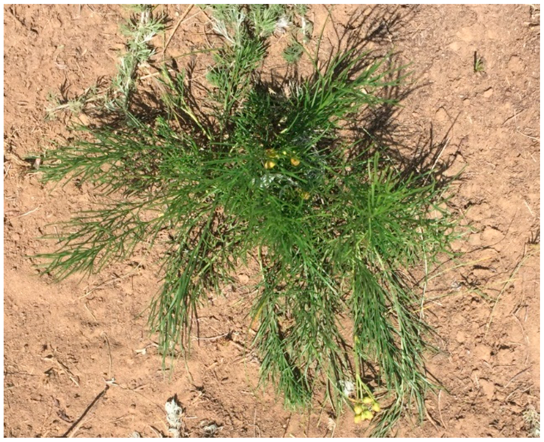
Polygonum divaricatum
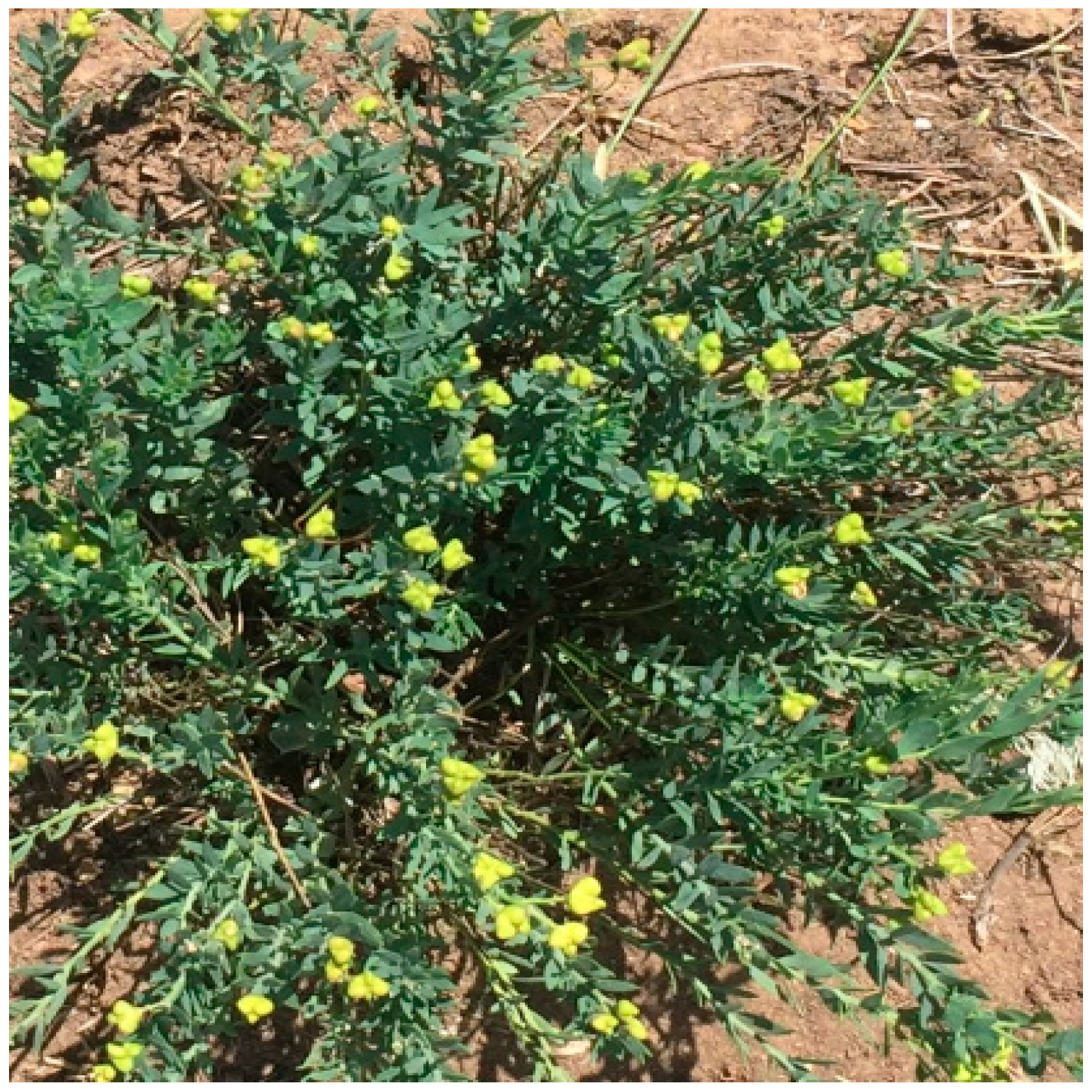
Haplophyllum dauricum
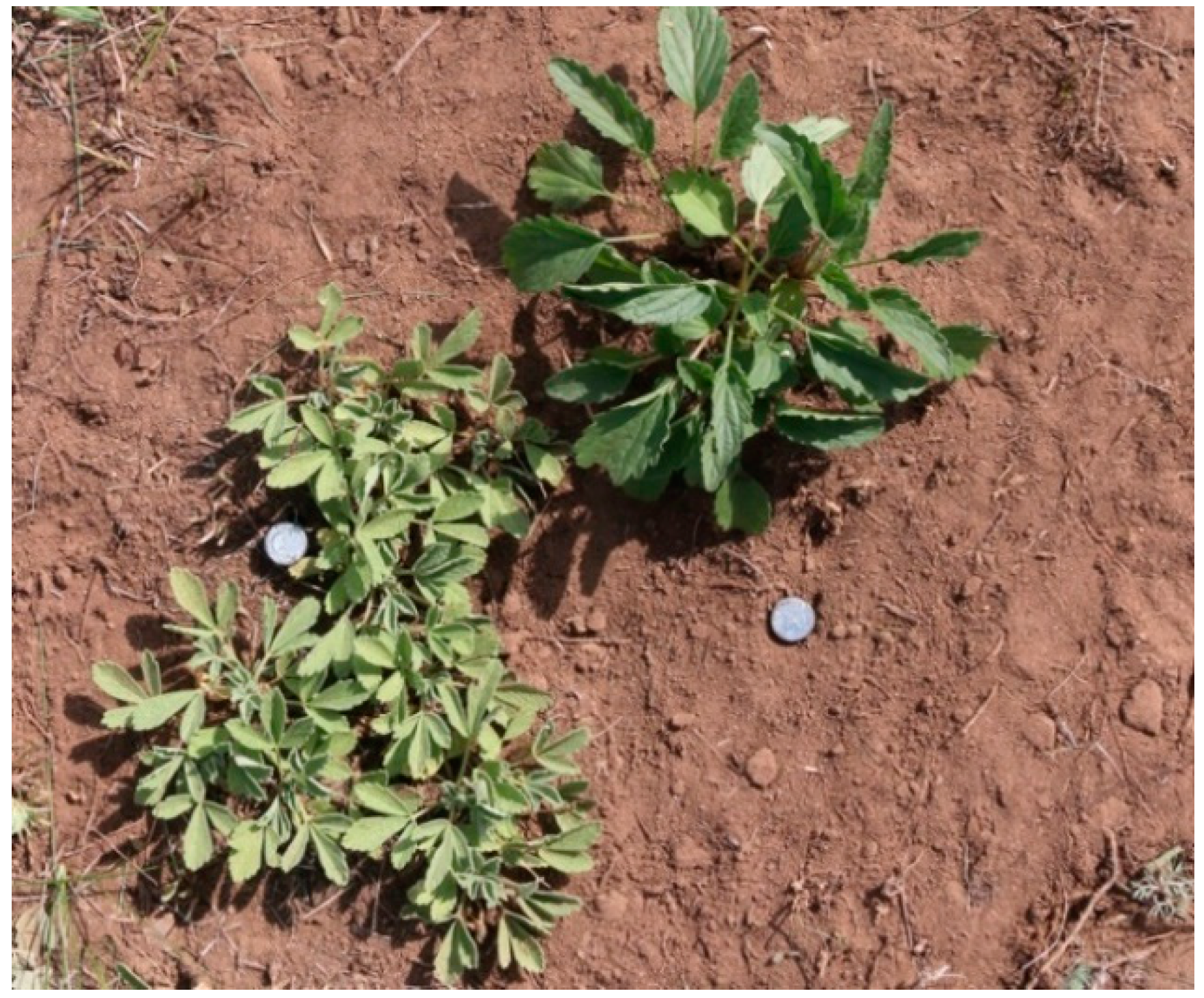
Potentilla chinensis
Cichorium intybus
Stipa capillata
Observation Target: Artemisia frigida
4.2.2. Experiment 2
5. Results and Discussion
5.1. Research on the Characteristics of the Emissivity Curves of Different Types of Grassland Vegetation Based on Experiment 1
5.1.1. Temperature and Emissivity Retrieval of Haplophyllum dauricum
5.1.2. Temperature and Emissivity Retrieval of Artemisia subulata Nakai and Stipa capillata
5.1.3. Temperature and Emissivity Retrieval of Potentilla chinensis
5.1.4. Temperature and Emissivity Retrieval of Cichorium intybus
5.1.5. Temperature and Emissivity Retrieval of Polygonum divaricatum
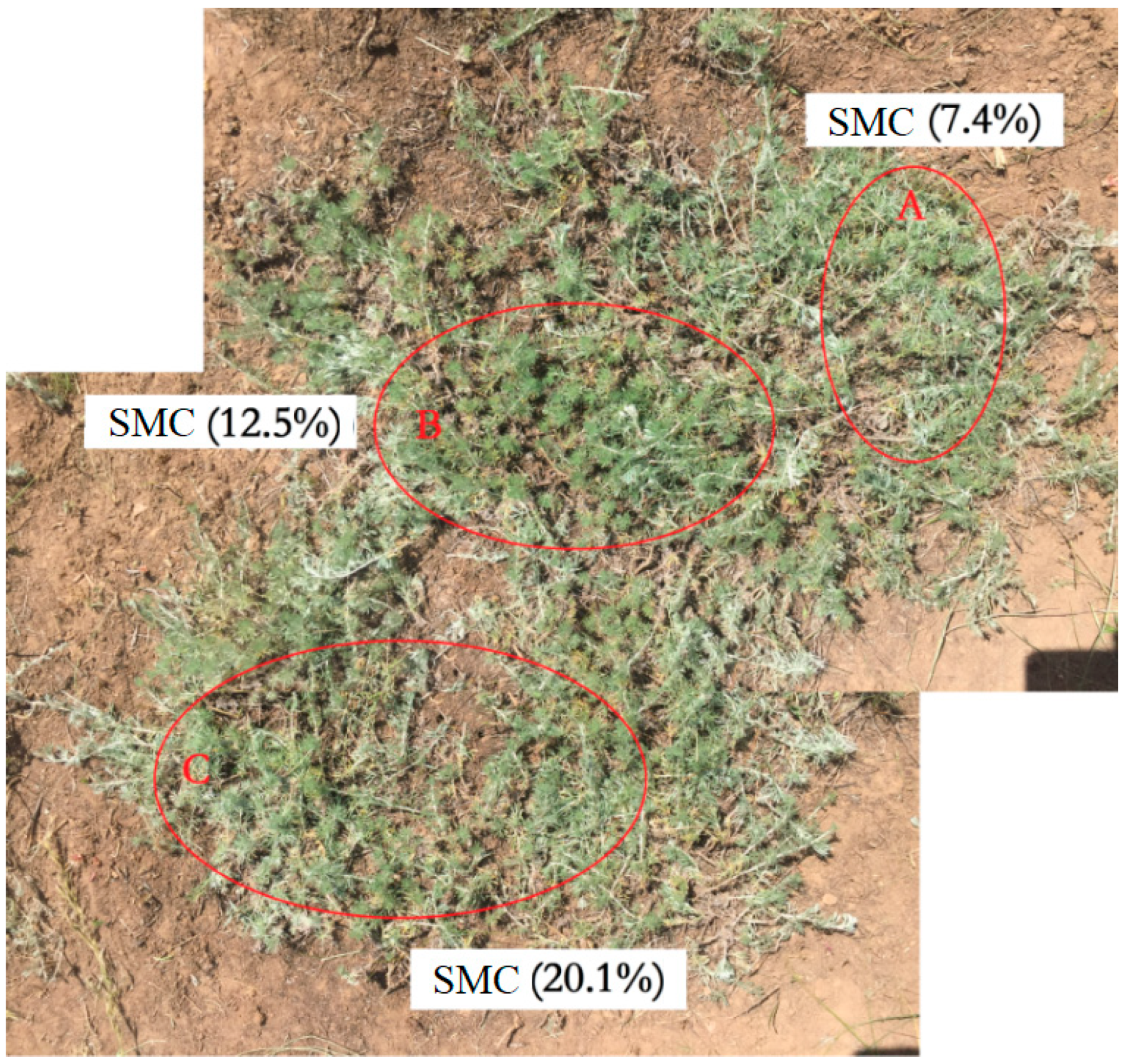
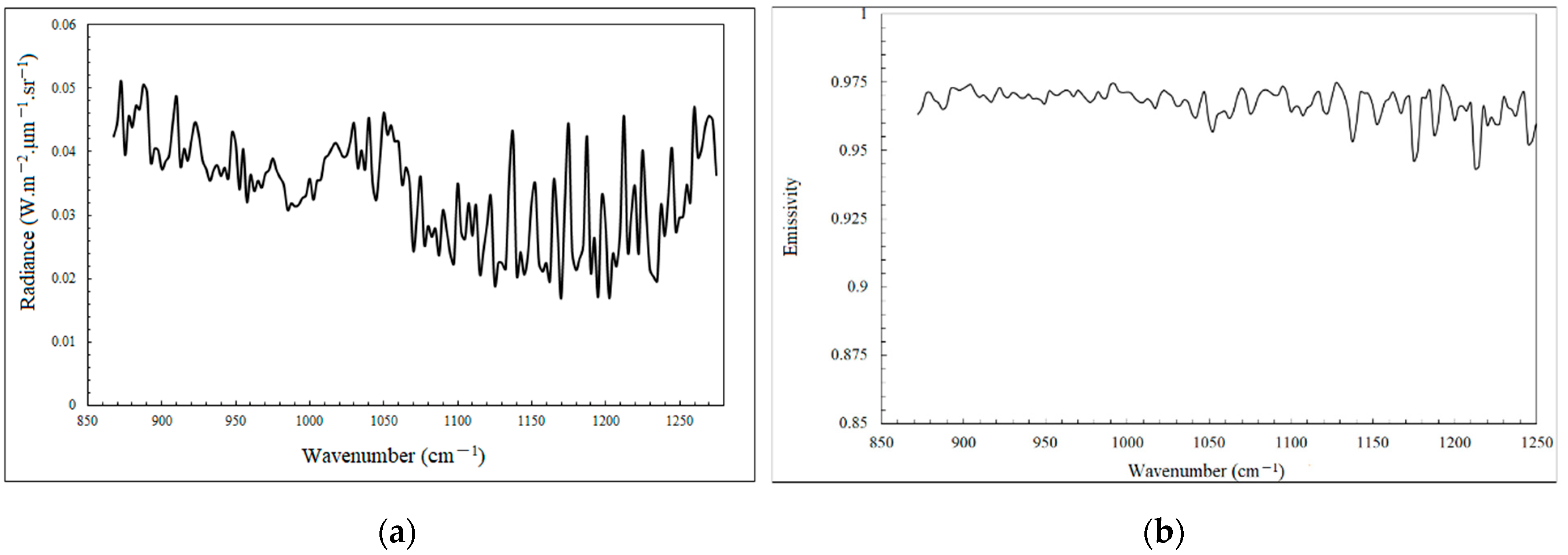
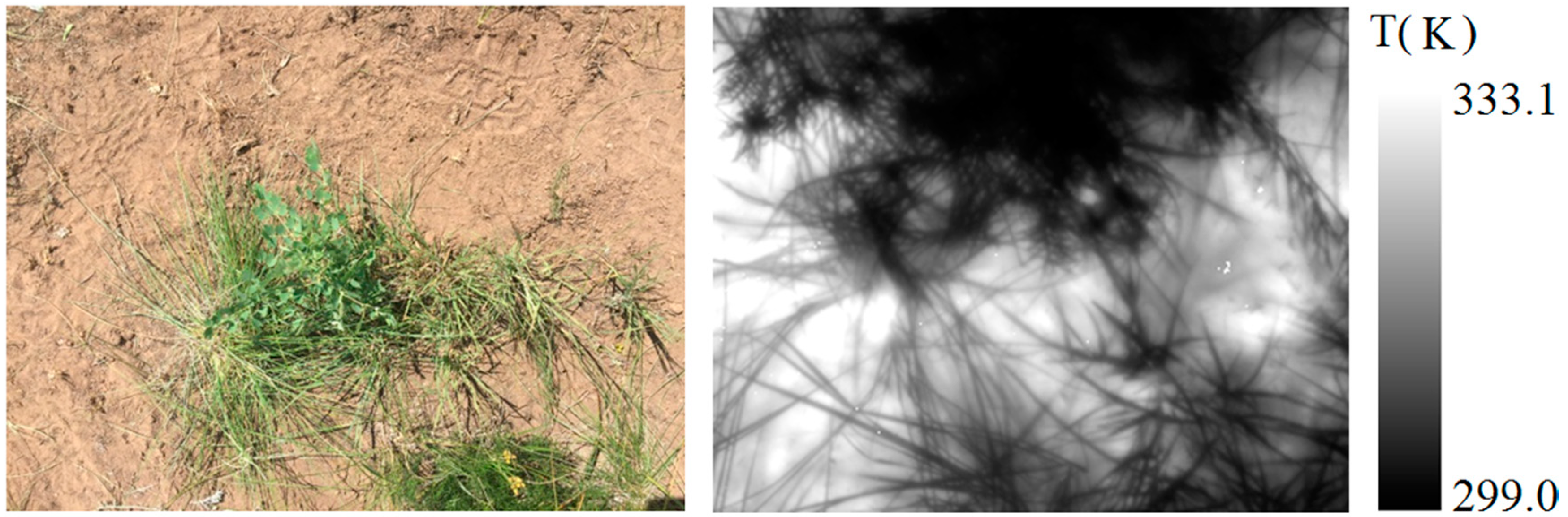
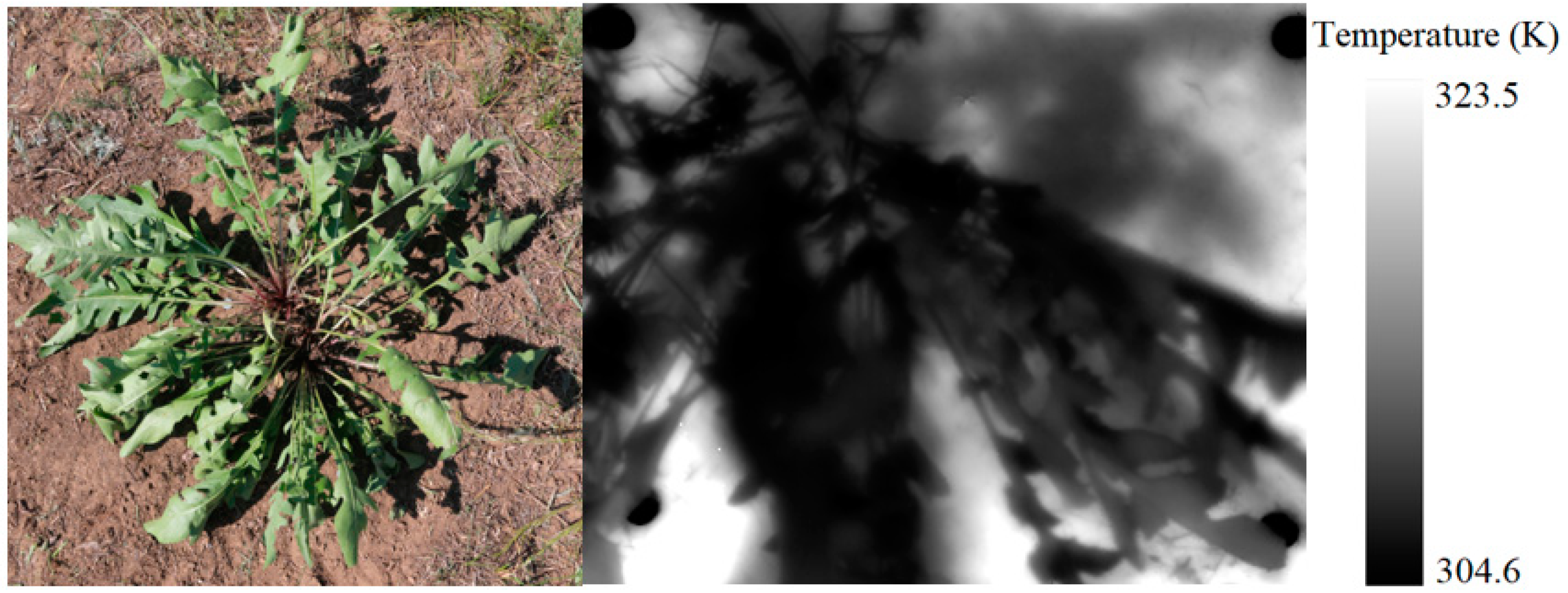
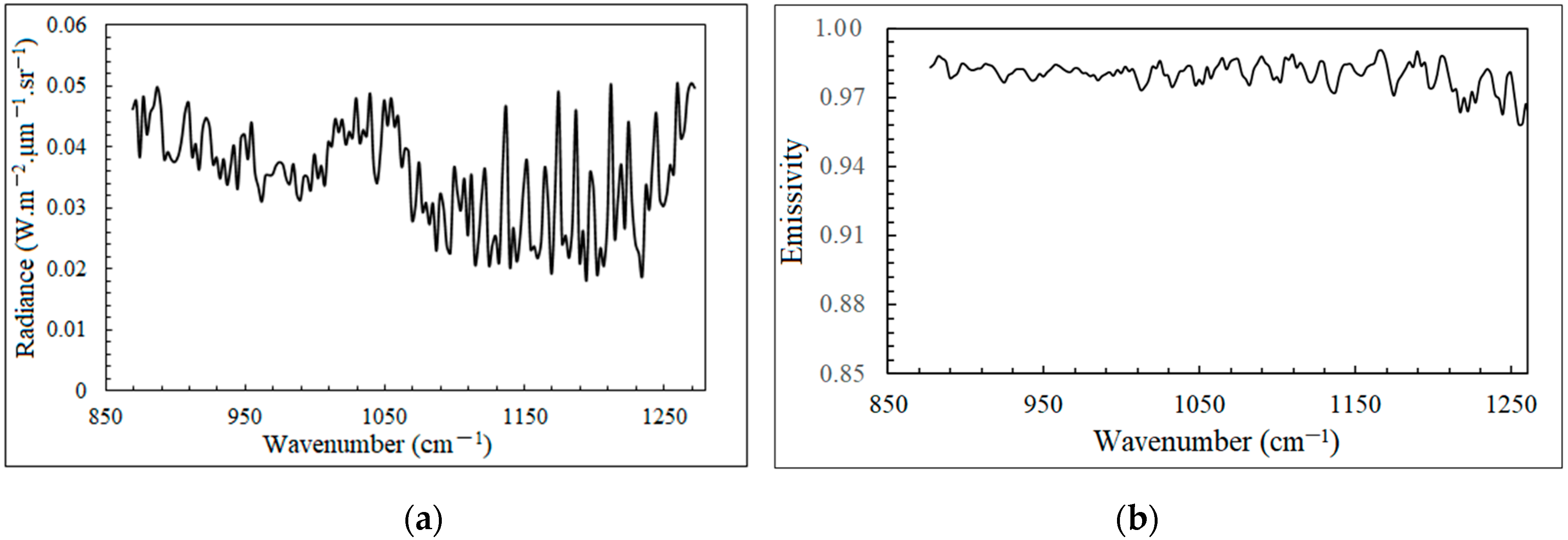
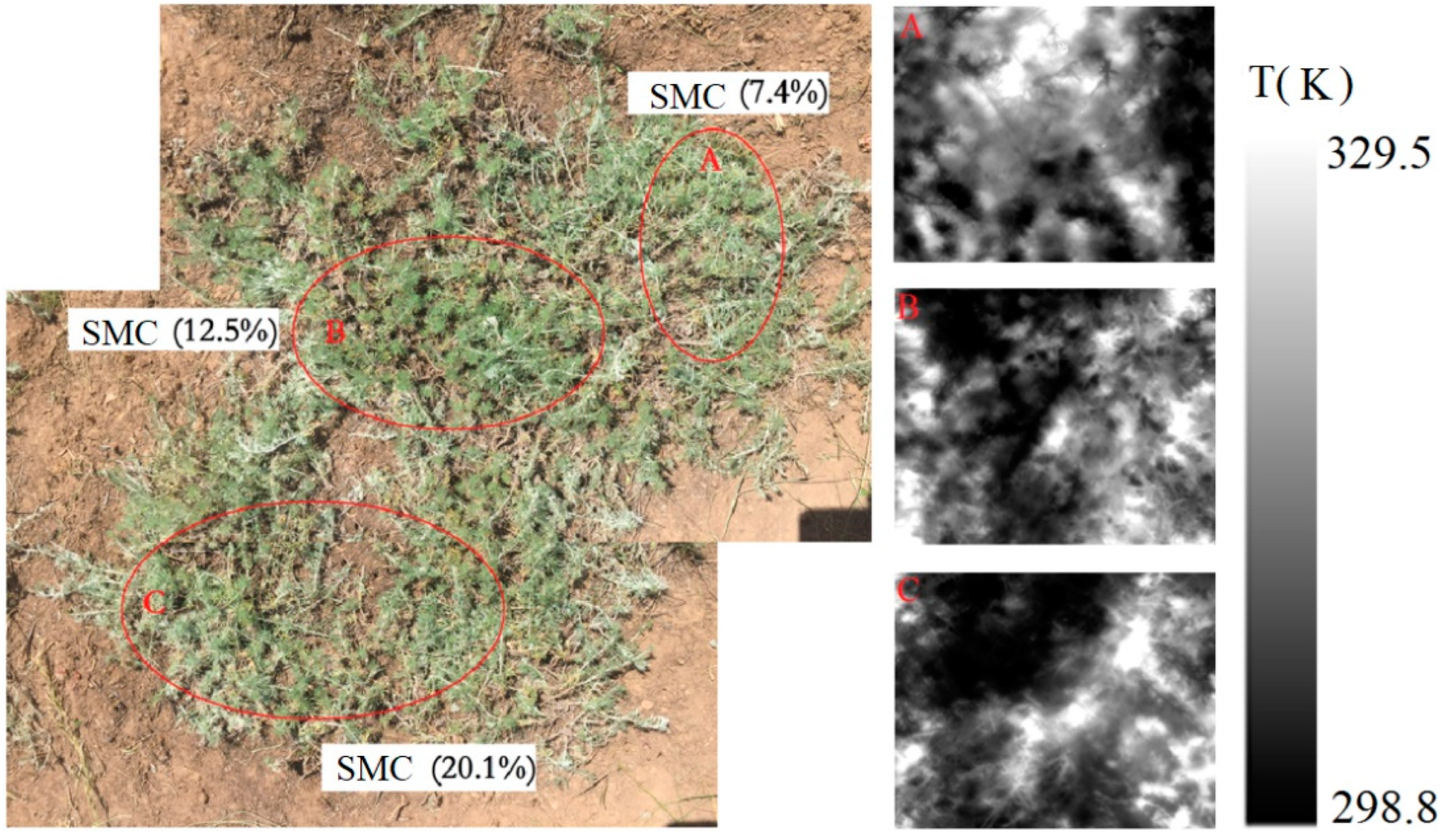
5.2. Characteristic Changes in the Emissivity of Artemisia annua under Different Moisture Conditions Based on Experiment 2
6. Conclusions and Suggestions
Author Contributions
Funding
Data Availability Statement
Conflicts of Interest
References
- Chaves, M.M.; Pereira, J.S.; Maroco, J.; Rodrigues, M.L.; Ricardo, C.P.; Osório, M.L.; Carvalho, I.; Faria, T.; Pinheiro, C. How plants cope with water stress in the field? Photosynthesis and growth. Ann. Bot. 2002, 89, 907–916. [Google Scholar] [CrossRef] [PubMed]
- Hopkins, W.G.; Huner, N.P.A. Responses of plants to environmental stresses. In Introduction to Plant Physiology; John Wiley & Sons, Inc.: Hoboken, NJ, USA, 2009; pp. 223–239. [Google Scholar]
- Ni, Z.; Liu, Z.; Huo, H.; Li, Z.L.; Nerry, F.; Wang, Q.; Li, X. Early Water Stress Detection Using Leaf-Level Measurements of Chlorophyll Fluorescence and Temperature Data. Remote Sens. 2015, 7, 3232–3249. [Google Scholar] [CrossRef]
- Ni, Z.; Huo, H.; Tang, S.; Li, Z.L.; Liu, Z.; Xu, S.; Chen, B. Assessing the response of satellite sun-induced chlorophyll fluorescence and MODIS vegetation products to soil moisture from 2010 to 2017: A case in Yunnan Province of China. Int. J. Remote Sens. 2019, 40, 2278–2295. [Google Scholar] [CrossRef]
- Chaerle, L.; Van Der Straeten, D. Imaging techniques and the early detection of plant stress. Trends Plant Sci. 2000, 5, 495–501. [Google Scholar] [CrossRef]
- Gebbers, R.; Adamchuk, V.I. Precision Agriculture and Food Security. Science 2010, 327, 828–831. [Google Scholar] [CrossRef]
- Mulla, D.J. Twenty five years of remote sensing in precision agriculture: Key advances and remaining knowledge gaps. Biosyst. Eng. 2013, 114, 358–371. [Google Scholar] [CrossRef]
- Huo, H.; Li, Z.L.; Xing, Z. Temperature/emissivity separation using hyperspectral thermal infrared imagery and its potential for detecting the water content of plants. Int. J. Remote Sens. 2019, 40, 1672–1692. [Google Scholar] [CrossRef]
- Pinter, P.J., Jr.; Hatfield, J.L.; Schepers, J.S.; Barnes, E.M.; Moran, M.S.; Daughtry, C.S.T.; Upchurch, D.R. Remote Sensing for Crop Management. Photogramm. Eng. Remote Sens. 2003, 69, 647–664. [Google Scholar]
- Ni, Z.; Lu, Q.; Huo, H.; Zhang, H. Estimation of Chlorophyll Fluorescence at Different Scales: A Review. Sensors 2019, 19, 3000. [Google Scholar] [CrossRef]
- Ni, Z.; Liu, Z.; Li, Z.-L.; Nerry, F.; Huo, H.; Li, X. Estimation of solar-induced fluorescence using the canopy reflectance index. Int. J. Remote Sens. 2015, 36, 5239–5256. [Google Scholar] [CrossRef]
- Ni, Z.; Liu, Z.; Li, Z.-L.; Nerry, F.; Huo, H.; Sun, R.; Yang, P.; Zhang, W. Investigation of Atmospheric Effects on Retrieval of Sun-Induced Fluorescence Using Hyperspectral Imagery. Sensors 2016, 16, 480. [Google Scholar] [CrossRef] [PubMed]
- Zhao, L.; Liu, Z.; Xu, S.; He, X.; Ni, Z.; Zhao, H.; Ren, S. Retrieving the Diurnal FPAR of a Maize Canopy from the Jointing Stage to the Tasseling Stage with Vegetation Indices under Different Water Stresses and Light Conditions. Sensors 2018, 18, 3965. [Google Scholar] [CrossRef] [PubMed]
- Rascher, U.; Alonso, L.; Burkart, A.; Cilia, C.; Zemek, F. Suninduced fluorescence—A new probe of photosynthesis: First maps from the imaging spectrometer HyPlant. Glob. Chang. Biol. 2015, 21, 4673–4684. [Google Scholar] [CrossRef] [PubMed]
- da Luz, B.R.; Crowley, J.K. Spectral reflectance and emissivity features of broad leaf plants: Prospects for remote sensing in the thermal infrared (8.0–14.0 μm). Remote Sens. Environ. 2007, 109, 393–405. [Google Scholar] [CrossRef]
- Seelig, H.-D.; Hoehn, A.; Stodieck, L.S.; Klaus, D.M.; Adams, W.W.; Emery, W.J. Relations of remote sensing leaf water indices to leaf water thickness in cowpea, bean, and sugarbeet plants. Remote Sens. Environ. 2008, 112, 445–455. [Google Scholar] [CrossRef]
- Dechant, B.; Ryu, Y.; Badgley, G.; Zeng, Y.; Berry, J.A.; Zhang, Y.; Goulas, Y.; Li, Z.; Zhang, Q.; Kang, M.; et al. Canopy structure explains the relationship between photosynthesis and sun-induced chlorophyll fluorescence in crops. Remote Sens. Environ. 2020, 241, 111733. [Google Scholar] [CrossRef]
- Meroni, M.; Rossini, M.; Guanter, L.; Alonso, L.; Rascher, U.; Colombo, R.; Moreno, J. Remote sensing of solar-induced chlorophyll fluorescence: Review of methods and applications. Remote Sens. Environ. 2009, 113, 2037–2051. [Google Scholar] [CrossRef]
- Porcar-Castell, A.; Tyystjarvi, E.; Atherton, J.; van der Tol, C.; Flexas, J.; Pfundel, E.E.; Moreno, J.; Frankenberg, C.; Berry, J.A. Linking chlorophyll a fluorescence to photosynthesis for remote sensing applications: Mechanisms and challenges. J. Exp. Bot. 2014, 65, 4065–4095. [Google Scholar] [CrossRef]
- Rossini, M.; Nedbal, L.; Guanter, L.; Ač, A.; Alonso, L.; Burkart, A.; Cogliati, S.; Colombo, R.; Damm, A.; Drusch, M. Red and far red Sun-induced chlorophyll fluorescence as a measure of plant photosynthesis. Geophys. Res. Lett. 2015, 42, 1632–1639. [Google Scholar] [CrossRef]
- Wieneke, S.; Ahrends, H.; Damm, A.; Pinto, F.; Stadler, A.; Rossini, M.; Rascher, U. Airborne based spectroscopy of red and far-red sun-induced chlorophyll fluorescence : Implications for improved estimates of gross primary productivity. Remote Sens. Environ. 2016, 184, 654–667. [Google Scholar] [CrossRef]
- Moran, M.S.; Inoue, Y.; Barnes, E.M. Opportunities and limitations for image-based remote sensing in precision crop management. Remote Sens. Environ. 1997, 61, 319–346. [Google Scholar] [CrossRef]
- Govender, M.; Dye, P.; Weiersbye, I. Review of commonly used remote sensing and groundbased technologies to measure plant water stress. Water SA 2009, 35, 741–752. [Google Scholar] [CrossRef]
- Jones, H.G.; Vaughan, R.A. Remote Sensing of Vegetation : Principles, Techniques, and Applications; Oxford University Press: Oxford, UK, 2010. [Google Scholar]
- Hunt, E., Jr.; Rock, B. Detection of changes in leaf water content using Near- and Middle-Infrared reflectances. Remote Sens. Environ. 1989, 30, 43–54. [Google Scholar]
- Peñuelas, J.; Gamon, J.A.; Fredeen, A.L.; Merino, J.; Field, C.B. Reflectance indicies associated with physiological changes in Nitrogen- and water- limited sunflower leaves. Remote Sens. Environ. 1994, 48, 135–146. [Google Scholar] [CrossRef]
- Jones, H.G. Application of Thermal Imaging and Infrared Sensing in Plant Physiology and Ecophysiology. In Advances in Botanical Research; Academic Press: Cambridge, MA, USA, 2004; pp. 107–163. [Google Scholar]
- Tardy, B.; Rivalland, V.; Huc, M.; Hagolle, O.; Marcq, S.; Boulet, G. A software tool for atmospheric correction and surface temperature estimation of Landsat infrared thermal data. Remote Sens. 2016, 8, 696. [Google Scholar] [CrossRef]
- Maes, W.H.; Steppe, K. Estimating evapotranspiration and drought stress with ground-based thermal remote sensing in agriculture: A review. J. Exp. Bot. 2012, 63, 4671–4712. [Google Scholar] [CrossRef]
- Costa, J.M.; Grant, O.M.; Chaves, M.M. Thermography to explore plant-environment interactions. J. Exp. Bot. 2013, 64, 3937–3949. [Google Scholar] [CrossRef]
- Maes, W.H.; Baert, A.; Huete, A.R.; Minchin, P.E.H.; Snelgar, W.P.; Steppe, K. A new wet reference target method for continuous infrared thermography of vegetations. Agric. For. Meteorol. 2016, 226–227, 119–131. [Google Scholar] [CrossRef]
- Jackson, R.D.; Reginato, R.J.; Idso, S.B. Wheat canopy temperature: A practical tool for evaluating water requirements. Water Resour. Res. 1977, 13, 651–656. [Google Scholar] [CrossRef]
- Idso, S.B.; Jackson, R.D.; Reginato, R.J. Remote sensing for agricultural water management and crop yield prediction. Agric. Water Manag. 1977, 1, 299–310. [Google Scholar] [CrossRef]
- Moran, M.S.; Clarke, T.R.; Inoue, Y.; Vidal, A. Estimating crop water deficit using the relation between surface-air temperature and spectral vegetation index. Remote Sens. Environ. 1994, 49, 246–263. [Google Scholar] [CrossRef]
- Jones, H.G. Use of thermography for quantitative studies of spatial and temporal variation of stomatal conductance over leaf surfaces. Plant Cell Environ. 1999, 22, 1043–1055. [Google Scholar] [CrossRef]
- Mallick, K.; Boegh, E.; Trebs, I.; Alfieri, J.G.; Kustas, W.P.; Prueger, J.H.; Niyogi, D.; Das, N.; Drewry, D.T.; Hoffmann, L.; et al. Reintroducing radiometric surface temperature into the P enman-M onteith formulation. Water Resour. Res. 2015, 51, 6214–6243. [Google Scholar] [CrossRef]
- Jones, H.G.; Serraj, R.; Loveys, B.R.; Xiong, L.; Wheaton, A.; Price, A.H. Thermal infrared imaging of crop canopies for the remote diagnosis and quantification of plant responses to water stress in the field. Funct. Plant Biol. 2009, 36, 978–989. [Google Scholar] [CrossRef] [PubMed]
- Grant, O.M.; Davies, M.J.; James, C.M.; Johnson, A.W.; Leinonen, I.; Simpson, D.W. Thermal imaging and carbon isotope composition indicate variation amongst strawberry (Fragaria × ananassa) cultivars in stomatal conductance and water use efficiency. Environ. Exp. Bot. 2012, 76, 7–15. [Google Scholar] [CrossRef]
- Leng, P.; Li, Z.-L.; Duan, S.-B.; Gao, M.-F.; Huo, H.-Y. First results of all-weather soil moisture retrieval from an optical/thermal infrared remote-sensing-based operational system in China. Int. J. Remote Sens. 2019, 40, 2069–2086. [Google Scholar] [CrossRef]
- Pei, L.; Li, Z.-L.; Duan, S.B.; Tang, R.; Gao, M.-F. A method for deriving all-sky evapotranspiration from the synergistic use of remotely sensed images and meteorological data. J. Geophys. Res. Atmos. 2017, 122, 13–263. [Google Scholar]
- Leng, P.; Li, Z.-L.; Duan, S.-B.; Gao, M.-F.; Huo, H.-Y. A practical approach for deriving all-weather soil moisture content using combined satellite and meteorological data. ISPRS J. Photogramm. Remote Sens. 2017, 131, 40–51. [Google Scholar] [CrossRef]
- Li, Z.L.; Leng, P.; Zhou, C.; Chen, K.S.; Zhou, F.C.; Shang, G.F. Soil moisture retrieval from remote sensing measurements: Current knowledge and directions for the future. Earth-Sci. Rev. 2021, 218, 103673. [Google Scholar] [CrossRef]
- Leng, P.; Liao, Q.Y.; Gao, M.F.; Duan, S.B.; Li, Z.L.; Zhang, X.; Shang, G.F. A full satellite-driven method for the retrieval of clear-sky evapotranspiration. Earth Space Sci. 2019, 6, 2251–2262. [Google Scholar]
- Wang, Y.; Leng, P.; Ma, J.; Peng, J. A Method for Downscaling Satellite Soil Moisture Based on Land Surface Temperature and Net Surface Shortwave Radiation. IEEE Geosci. Remote Sens. Lett. 2022, 19, 3002105. [Google Scholar] [CrossRef]
- Zarco-Tejada, P.J.; González-Dugo, V.; Williams, L.E.; Suárez, L.; Berni, J.A.; Goldhamer, D.; Fereres, E. 2013. A PRI-based water stress index combining structural and chlorophyll effects: Assessment using diurnal narrow-band airborne imagery and the CWSI thermal index. Remote Sens. Environ. 2013, 138, 38–50. [Google Scholar] [CrossRef]
- Ullah, S.; Skidmore, A.K.; Naeem, M.; Schlerf, M. An accurate retrieval of leaf water content from mid to thermal infrared spectra using continuous wavelet analysis. Sci. Total Environ. 2012, 437, 145–152. [Google Scholar] [CrossRef] [PubMed]
- Salisbury, J.W. Preliminary measurements of leaf spectral reflectance in the 8–14 μm region. Int. J. Remote Sens. 1986, 7, 1879–1886. [Google Scholar] [CrossRef]
- da Luz, B.R.; Crowley, J.K. Identification of plant species by using high spatial and spectral resolution thermal infrared (8.0–13.5 μm) imagery. Remote Sens. Environ. 2010, 114, 404–413. [Google Scholar] [CrossRef]


| Habitat Distribution Types | Cosmopolitan | Pantropic | Temperate | |
|---|---|---|---|---|
| Plant Species Types | ||||
| Carex Meadow | 70.8% | 4.2% | 20.8% | |
| Typical Steppe | 85% | 5% | 10% | |
| Sandy Vegetation | 69.2% | 7.7% | 23.1% | |
| Artificial Populus Davidiana Forests | 75% | 10% | 15% | |
| Salix Pentandra Meadow | 82.4% | 7.6% | ||
| Achnatherum Splendens Meadow | 87.5% | 12.5% | ||
| Parameters | Unit | Mini. | Typical | Max. |
|---|---|---|---|---|
| Spectral range | μm | 8 | 11 | |
| Spectral resolution | cm−1 | 0.25 | 4 | 150 |
| Spatial resolution | pixels | 320 × 256 | ||
| Single beam FOV | Mrad | 0.35 | ||
| Noise equivalent | nW/cm2 sr cm−1 | 25 at 10 um | ||
| Radiometric accuracy | K | <1 | ||
| Commucation | Ethernet 10/100 Mbps | Ethernet 10/100 Mbps | ||
| Data transfer | Cameral Link | |||
| Detector cooling | Closed Cycle | |||
| Weight | kg | 27 |
Publisher’s Note: MDPI stays neutral with regard to jurisdictional claims in published maps and institutional affiliations. |
© 2022 by the authors. Licensee MDPI, Basel, Switzerland. This article is an open access article distributed under the terms and conditions of the Creative Commons Attribution (CC BY) license (https://creativecommons.org/licenses/by/4.0/).
Share and Cite
Liu, P.; Huo, H.; Guo, L.; Leng, P.; He, L. Temperature/Emissivity Separation of Typical Grassland of Northwestern China Based on Hyper-CAM and Its Potential for Grassland Drought Monitoring. Remote Sens. 2022, 14, 4809. https://doi.org/10.3390/rs14194809
Liu P, Huo H, Guo L, Leng P, He L. Temperature/Emissivity Separation of Typical Grassland of Northwestern China Based on Hyper-CAM and Its Potential for Grassland Drought Monitoring. Remote Sensing. 2022; 14(19):4809. https://doi.org/10.3390/rs14194809
Chicago/Turabian StyleLiu, Pengfei, Hongyuan Huo, Li Guo, Pei Leng, and Long He. 2022. "Temperature/Emissivity Separation of Typical Grassland of Northwestern China Based on Hyper-CAM and Its Potential for Grassland Drought Monitoring" Remote Sensing 14, no. 19: 4809. https://doi.org/10.3390/rs14194809
APA StyleLiu, P., Huo, H., Guo, L., Leng, P., & He, L. (2022). Temperature/Emissivity Separation of Typical Grassland of Northwestern China Based on Hyper-CAM and Its Potential for Grassland Drought Monitoring. Remote Sensing, 14(19), 4809. https://doi.org/10.3390/rs14194809