Article

Satellite and High-Spatio-Temporal Resolution Data Collected by Southern Elephant Seals Allow an Unprecedented 3D View of the Argentine Continental Shelf

by
Melina M. Martinez
1,2,3,*,
Laura A. Ruiz-Etcheverry
1,2,3,
Martin Saraceno
1,2,3,
Anatole Gros-Martial
4,5,6,
Julieta Campagna
7,
Baptiste Picard
6 and
Christophe Guinet
6
1
Departamento de Ciencias de la Atmósfera y los Océanos (DCAO), Facultad de Ciencias Exactas y Naturales, Universidad de Buenos Aires, Buenos Aires C1428EGA, Argentina
2
Centro de Investigaciones del Mar y la Atmósfera (CIMA), CONICET—Universidad de Buenos Aires, Buenos Aires C1428EGA, Argentina
3
Instituto Franco-Argentino de Estudios sobre el Clima y sus Impactos (IFAECI), IRL 3351, CNRS-CONICET-IRD-UBA, Buenos Aires C1428EGA, Argentina
4
ENSTA-Bretagne, UMR6285 Lab-STICC, F-29200 Brest, France
5
CNRS, Ifremer, IUEM, University Brest, UMR6538 Geo-Ocean, F-29280 Plouzané, France
6
Centre d’Etudes Biologiques de Chizé, UMR 7372, CNRS-La Rochelle Université, F-79360 Villiers en Bois, France
7
Wildlife Conservation Society, Argentina, and Marine Programs, Amenábar 1595, Buenos Aires 1426, Argentina
*
Author to whom correspondence should be addressed.
Remote Sens. 2023, 15(23), 5604; https://doi.org/10.3390/rs15235604
Submission received: 4 October 2023 / Revised: 25 November 2023 / Accepted: 26 November 2023 / Published: 2 December 2023
(This article belongs to the Special Issue Oceans from Space V)

Abstract

:
High spatial and temporal resolution hydrographic data collected by Southern Elephant Seals (Mirounga leonina, SESs) and satellite remote sensing data allow a detailed oceanographic description of the Argentine Continental Shelf (ACS). In-situ data were obtained from the CTD (Conductivity, Temperature, and Depth), accelerometer, and hydrophone sensors attached to five SESs that crossed the ACS between the 17th and 31st of October 2019. The analysis of the temperature (T) and salinity (S) along the trajectories allowed us to identify two different regions: north and south of 42°S. Satellite Sea Surface Temperature (SST) data suggests that north of 42°S, warm waters are coming from the San Matias Gulf (SMG). The high spatio-temporal resolution of the in-situ data shows regions with intense gradients along the T and S sections that were associated with a seasonal front that develops north of Península Valdés in winter due to the entrance of cold and fresh water to the SMG. The speed of the SESs is correlated with tidal currents in the coastal portion of the northern region, which is in good agreement with the macrotidal regime observed. A large number of Prey Catch Attempts (PCA), a measure obtained from the accelerometer sensor, indicates that SESs also feed in this region, contradicting suggestions from previous works. The analysis of wind intensity estimated from acoustic sensors allowed us to rule out the local wind as the cause of fast thermocline breakups observed along the SESs trajectories. Finally, we show that the maximum depth reached by the elephant seals can be used to detect errors in the bathymetry charts.

Graphical Abstract

1. Introduction

In the southern hemisphere (SH), one of the main limitations to understanding the marine environment is the scarce availability of in-situ data. Traditionally, in-situ observations of the marine environment are collected from research vessels, drifting buoys, and moorings. In recent decades, several animals have been used as autonomous platforms to collect oceanographic data, contributing to better sampling of the SH [1]. The use of diving animals allows for the best spatial and temporal resolution in the SH [2,3].
Thanks to the fact that Southern Elephant Seals (SESs) dive almost continuously [4] to deep waters (up to 2000 m) [5,6], on the order of 60 times per day [3,7], and travel thousands of kilometers [8,9], they represent excellent platforms to measure data in the water column of the ocean. SESs show strong site fidelity, returning reliably to natal breeding grounds twice a year, allowing for both attachment and recovery of instruments. The in-situ data collected allows us to study in detail the behavior of those animals and, simultaneously, allows us to evaluate the seasonal and interannual variability of key oceanographic parameters [9].
SESs colonies are located within the Antarctic Circle, except for the one located at Península Valdés (PV), in South America (Figure 1). While at sea, the spatial distribution of females and males is quite different [10]. Males forage mostly on the Patagonian shelf [11] and females mainly along the Patagonian shelf slope, shelf break, or Argentine Basin [12,13,14,15]. SESs females breed between late August and November and molt between December and January along ca. 200 km of open ocean coastline at PV [16,17]. SESs have been instrumented in PV since 1992 [14]. The oceanographic data collected by the PV colony have been used to study mesoscale structures in the open ocean [18], identify foraging places [12], and relate the species that the SESs eat to different water masses along the Patagonian shelf slope [13]. Based on the SESs path, speed, and swimming pattern, Campagna et al. [14] suggested that the shelf area is mainly a transit zone and is not the preferred feeding ground of the SESs females of PV. This was recently confirmed by McGovern et al. [15]. Here we propose to use T and S data to characterize the oceanographic conditions along the trajectories of the SESs within the continental shelf, taking advantage of the fact that they crossed it very fast. Indeed, the high-resolution profile data collected by SESs will provide a synoptic description of the oceanographic conditions of the Argentine Continental Shelf (ACS) adjacent to PV.
We focus our study on the region from the PV coast to the edge of the Patagonian shelf slope (defined by the 200 m isobath) from 55°W to 65°W and from 45°S to 41°S (Figure 1). The portion of ACS adjacent to PV is subject to different dynamics: In the eastern boundary, the Malvinas Current (MC) flows northward over the continental slope, carrying cold, nutrient-rich water. At 41°S, the slope water signal can be observed up to the mid-shelf due to MC intrusions [19]. In the western boundary, the PV tidal front is the main characteristic. The PV front is associated with transitioning between homogeneous coastal waters and vertically stratified mid-shelf waters during spring and summer [20,21]. The homogeneous coastal waters are the product of vertical mixing generated by energetic tidal currents, while the seasonal stratification on the mid-shelf is due to surface warming during spring and summer. The position of the PV front is strongly linked to the bottom topography [22,23], with a NE-SW alignment, following approximately the 75 m isobath between 41°S and 45°S [24,25]. This study area is affected by the MC and by the strong tides in the coastal region, as well as by the circulation of the San Matias Gulf (SMG). This gulf, a semi-enclosed coastal basin, is a source of salty and warm water due to the bathymetry and the current dynamics. Cold and relatively fresh shelf waters enter through the southeastern portion of the mouth mainly in winter and spring [26] and re-circulate within the SMG, gaining heat and salinity through solar heating and evaporation, respectively [27]. The warm and salty waters exported through the northern portion of the gulf mouth to the inner shelf are known as High-Salinity Coastal Waters (>34) [20,28,29]. The other water masses present in the ACS are Mid-Continental Shelf Water, which has a salinity between 33.4 and 33.8 [29,30], Coastal Water (Low Salinity, <33.4), and Malvinas Water (>33.8). Salinity is usually used in ACS to classify water masses [29,31].
The brief oceanographic description of the region presented here is based on the use of remote sensing data, numerical model outputs, and a few in-situ data obtained during oceanographic cruises. As we show below, the high-resolution in-situ data obtained with the instruments mounted on the SESs offer new, three-dimensional observations at a very fine scale resolution in the region, allowing to distinguish small fronts almost not described previously in the literature, which might be crucial in the CO2 flux dynamics. Thus, the aim of this study is to provide an updated and detailed oceanographic description of the PV region using this unique dataset in combination with satellite data. This work also aims to relate the environmental changes to SESs foraging behavior. The article is organized as follows: the data and methods are described in Section 2. Section 3 presents the results. Finally, Section 4 present the discussion and the main conclusions.

2. Materials and Methods

2.1. In-Situ Data

In-situ data used in this work have been collected as part of an international collaboration between the Centre National de la Recherche Scientifique (CNRS), the Wildlife Conservation Society (WCS), the University of Tasmania (UTAS), and the University of Buenos Aires (UBA). We analyzed data collected by 5 Southern elephant seals (SESs hereafter, Mirounga leonina) females that were equipped with Conductivity-Temperature-Depth Satellite Relay Data Loggers (CTD-SRDLs) between October 17 and 31, 2019 in PV, Argentina. Three biologging devices were glued to the animals before their departure to the sea for their post-breeding foraging trip (Table 1 and Table 2, Figure 2): a head-mounted DTAG-4 tag (configured as either a sound and movement tag, 97 × 55 × 33 mm, 200 g in air, n = 10, or a sonar and movement tag, 95 × 55 × 37 mm, 200 g in the air), a back-mounted Satellite Relayed Data Logger (CTD-SRDL, Sea Mammal Research Unit (SMRU), St Andrews, UK, 115 × 100 × 40 mm, 680 g in the air), and a neck-mounted Argos location-only satellite tag (SPOT, Wildlife Computers, Redmond, WA, USA, 72 × 54 × 24 mm, 119 g in the air).
The CTD-SRDL records salinity derived from conductivity, temperature, and pressure in hydrographic profiles. When the animals reach the surface, the data collected along the profiles is compressed and sent via messages, along with the positional information, through the Advanced Research and Global Observation Satellite (ARGOS) (http://www.argos-system.org/, accessed on 3 May 2021) [32]. The transmission occurs several times per day. The CTD-SRDL archives pressure, temperature, and salinity data recorded continuously throughout the foraging trip at 0.5 Hz for internal memory. This is far more frequent than the transmitted data (i.e., 3 to 4 24-T/S point profiles per day), but this requires the tags to be recovered when SESs come back to shore to molt in the summer (December–January) [1]. The typical accuracies are ±0.02 °C for temperature and ±0.05 or better for salinity [33]. Additionally, the SPOT tag was included to facilitate the recovery of the instruments when the animal returned to land in case the CTD-SDRL had stopped transmitting.
Acceleration measurements associated with the head-mounted DTAG-4 movement tag provide an index of prey capture attempts (PCA) [34]. This variable is considered the most reliable proxy for foraging success [35,36]. It offers the opportunity to link variations in elephant seal movements, diving, and foraging behavior with environmental conditions. The wind estimation can be obtained from the sound tag, which is derived from the absolute sound pressure following [37]. The DTAG-4 is also equipped with accurate location sensors that provide depth, longitude, and latitude data. The depth data were sampled at a frequency of 0.2 s, while the latitude and longitude data were sampled intermittently, with a variable sampling rate ranging from 1e-5 to 0.1 s. GPS (Global Positioning System) positions were obtained at each surfacing. At-sea movements were monitored using the ARGOS satellite-tracking system, and the loggers were recovered as soon as the seals hauled out for molting. The geolocation accuracy provided by satellite using ARGOS is ±5 km [38,39] and using GPS is about 50 m [40,41]. The CTD and sonar tags were synchronized by matching the depth data sampled by their respective pressure sensors, according to Le Bras et al. [42]. The environmental data are collected up to 50 Hz (Table 2). To compute the vertical profile data, we followed the procedure described in Siegelman et al. [43]: First, temperature and conductivity are corrected for a thermal mass effect; then salinity spiking and density inversion are removed by adjusting salinity while leaving temperature unchanged.
The methodology used for the colocation of instruments on SESs is described by Campagna et al. [44]. The loggers are noninvasive [45]; they are glued to the animal’s hair and fall off when it molts. Furthermore, elephant seals’ performances do not appear to be impacted by loggers [46]. Thanks to the satellite tag, the tools are recovered when the animals return to shore. After recovering, the data collected were calibrated following the methodology described by Roquet et al. [45] and Sigelman et al. [43].

2.2. Satellite Data

Sea Surface Temperature (SST) from the Multi-scale Ultra-High Resolution L4 product (MUR—https://podaac.jpl.nasa.gov/MEaSUREs-MUR, accessed on 31 August 2021) with daily resolution and spatial resolution of 0.011° × 0.011° is used to compare the surface temperature obtained by the SESs. This high spatial resolution product is generated by combining MODIS, AVHRR, GOES, AMSR-E, and TMI measurements through the technique known as multi-resolution variational analysis [47]. The choice of this product is due to its high spatial resolution, and it has been successfully compared with independent in-situ data in this study region [48,49].

2.3. Reanalysis Data

Surface wind speed values are obtained from ECMWFs reanalysis model, ERA5. Reanalysis data are the product of a physics-based model combined with in-situ and satellite data [50]. More precisely, the integrated forecasting system has a 4D-variational assimilation with 12 h long windows and 12 min time steps [51] and uses data such as French RADOME, Land SYNOP, quickSCAT, and ASCAT as observations [52]. It gives hourly data on a 0.25° grid. The model provides an estimation of the 10 m wind, which is the wind speed ten meters above the surface.

2.4. Bathymetry Data

We used three gridded bathymetry dataset versions (2019, 2020, and 2021) of the General Bathymetric Chart of the Oceans (GEBCO) that are available at https://www.gebco.net/, accessed on 1 July 2021. All versions have been developed through the Nippon Foundation-GEBCO Seabed 2030 Project, which brings together all available bathymetric data to produce a map of the world ocean floor. The GEBCO 2019 portion of the ACS that we used has been corrected, considering bathymetry measurements provided by the Servicio de Hidrografia Naval. This version is currently the most used for regional numerical models in the region [26,53,54].

2.5. Tidal Model

TPXO is a global tidal model that provides a spatial resolution of 1/30°. The model assimilates satellite data from Topex Poseidon, Topex Tandem, ERS, GFO, and other data sets (i.e., tide gauges, ship-born ADCP). The model has a toolbox for accessing the coefficients for tidal harmonic constituents in barotropic tide models and for making predictions of tide height and currents [55]. TPXO8 is used to compare the zonal component velocity obtained by the SESs. The ACS presents a complex tidal region that is largely dominated by the semi-diurnal lunar constituent M2 [20,31]. TPXO8 represents tides very well in the region [56]. It has also been used to implement regional models [26,54].

2.6. Methodology

Several considerations must be considered to compare satellite SST with in-situ data. First, in-situ data are reliable at 15 m depth [35], not at the sea surface, where satellite data indicate SST. Second, satellite images of SST are typically available only once a day, while SESs conduct a vertical profile every 16 min and every 1.1 km on average over the continental shelf and therefore offer about 90 values every day in a large area. Hence, we extracted the nearest value, in time and space, of the satellite images to the 15 m in-situ data. Pearson correlations between both data sets are computed at a 95% confidence level. To evaluate the dispersion between both datasets, biases were calculated for each trajectory as follows:
BIAS = TMur − Tin-situ
The potential temperature and potential density were calculated using the Gibbs Sea Water (GSW) oceanographic toolbox [57] that considers the Thermodynamic Equation of Seawater 2010 (TEOS-2010).

3. Results

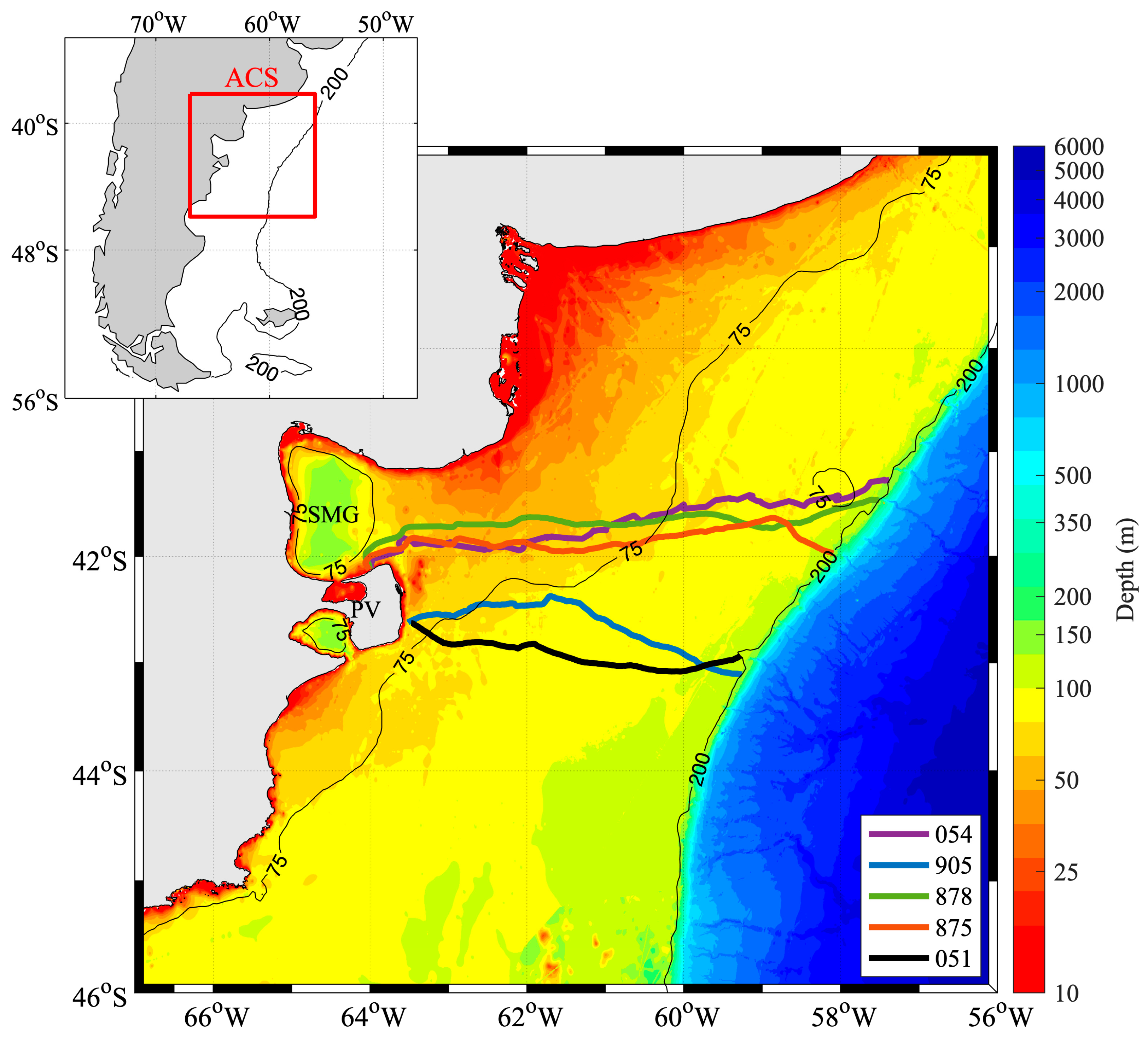
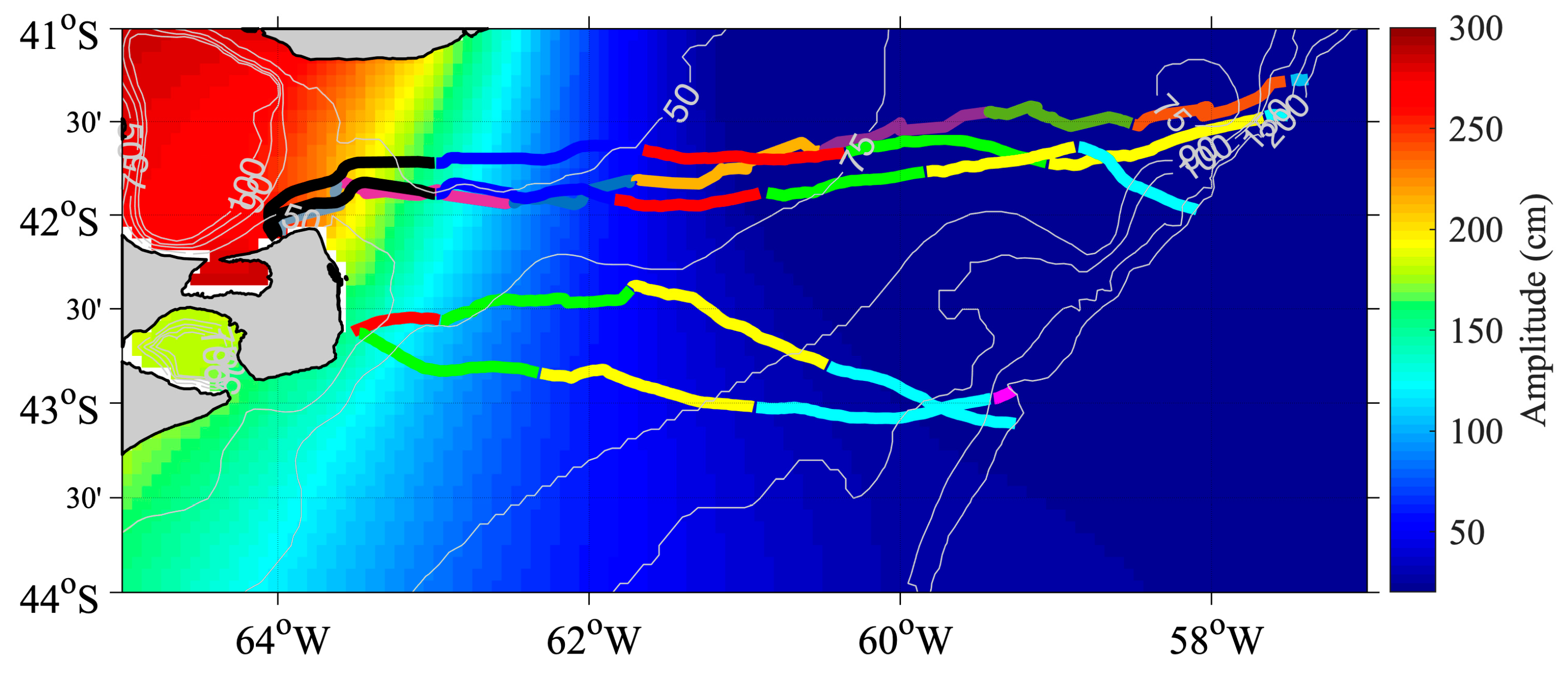
3.1. SESs Trajectories
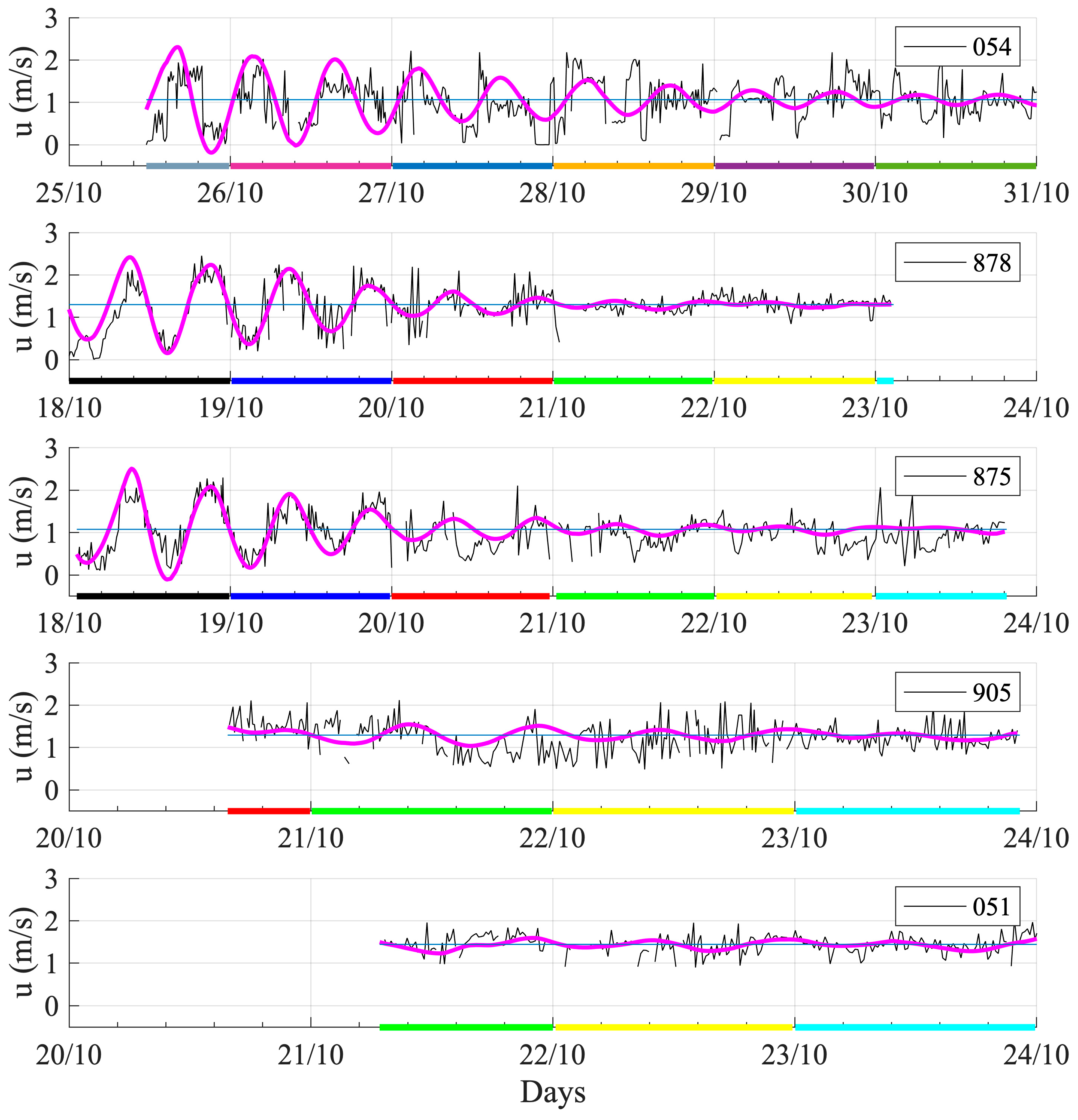
Figure 1 displays the trajectories of the five SESs analyzed in this work. SESs moved mainly towards the east from PV, reaching the open ocean in three to six days. The average number of dives per day on the continental shelf was 92.6 ± 10.2, and the average distance traveled per day was 110.1 ± 13.8 km (Table 3). The five SESs left PV and returned to molt to sites located very close to the place of departure in PV, between 21 December 2019, and 3 January 2020.
Table 3 summarizes basic statistics for the trajectories of the five elephant seals. All the SESs traveled a similar distance per day. The SESs that left from the north of PV (SESs 054, 878, 875) took more days to arrive at the 200 m isobath compared to the SESs that went from the south of PV (SESs 905, 051) because they traveled a longer distance to reach the eastern limit of the ACS, the 200 m isobath (Figure 1). In the following section, we analyze the speed of SESs along their trajectory in more detail.

3.2. SESs Speeds

Figure 3 shows the amplitude of the M2 tidal component and the trajectory of the SESs. M2 is the largest tidal component in the region, leading other components by an order of magnitude almost everywhere [31]. The three SESs left from the northern coast of PV crossed a portion of the ACS where the M2 tidal amplitude values were much greater than those along the trajectories of the SESs that left PV from the south (Figure 3). The speed of the zonal component of the tidal currents (considering all the tidal components of the TPXO8 model) along the trajectory of each SES is compared with the zonal speed of the animals in Figure 4. Both time series present similar variability during the three days after departure for the three northern elephants (054, 878, and 875); this feature is not observed in the two southern elephants (905 and 051). We can therefore observe that SES speed is largely correlated to tidal currents when the latter are large (>150 cm/s). It is an open question whether the SESs are taking advantage of the tidal currents or are affected by them.

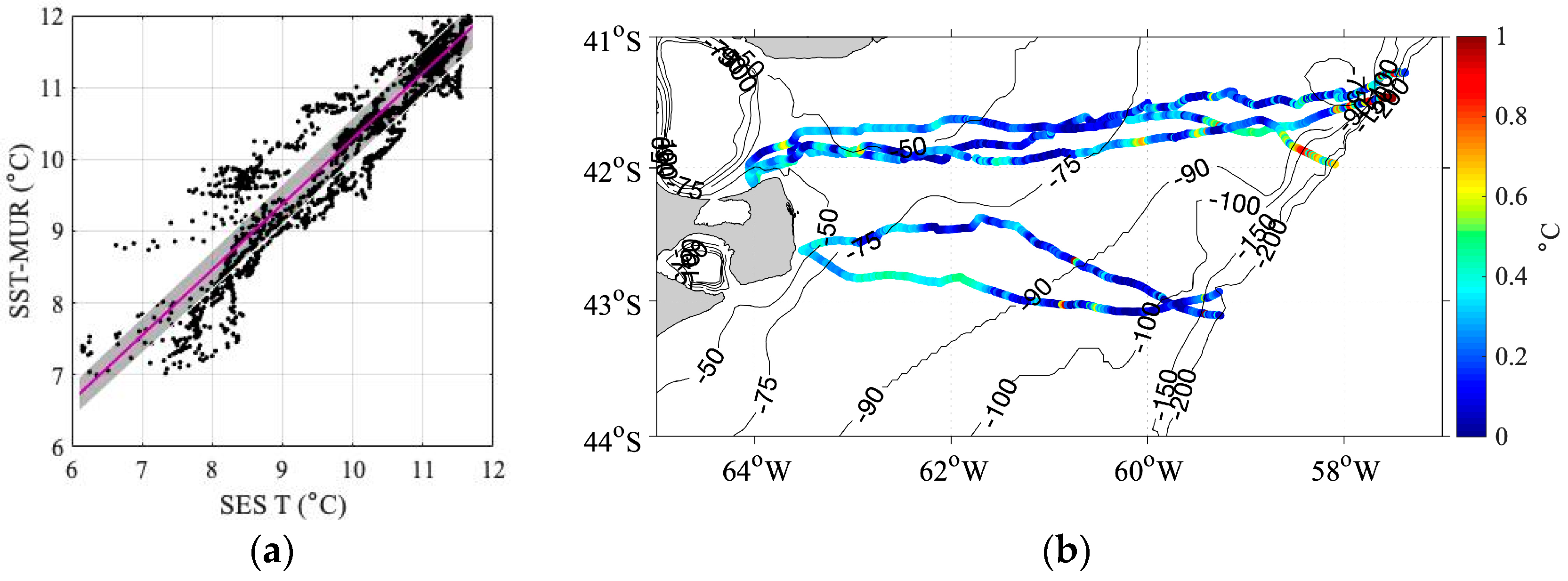
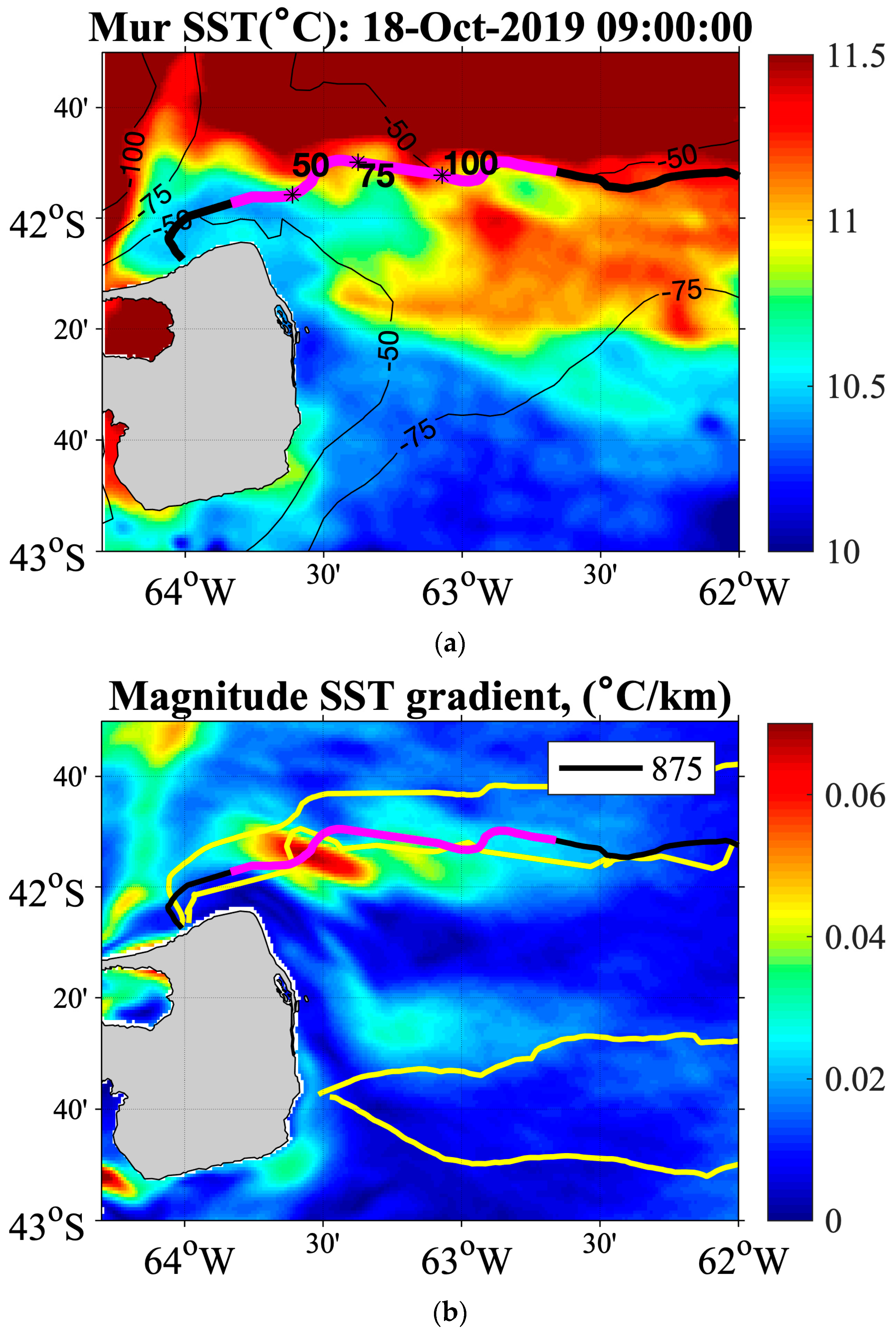
3.3. Comparison between Near-Surface SES Temperatures and Satellite SST

Figure 5 shows the scatterplot and the spatial distribution of the difference between the satellite and in-situ temperature datasets. The correlation between the near-surface temperature (15 m depth) collected by the SESs and the time-space matching SST is 0.97, significant at the 95% confidence level (CL95%).
Despite the good correlation between in-situ and satellite SST, the two datasets show a moderate dispersion in temperature values lower than 8 °C along the linear regression (Figure 5a). The differences are reflected in the bias values (Equation (1)) that, in general, are less than 0.5 °C, except in some parts of the trajectories, mainly near the shelf-break. (Figure 5b). Note that the bias values in all trajectories are positive. This means that the in-situ temperatures are lower than the SST-MUR. At first glance, this is an expected result since in-situ data are collected at 15 dbar, while the satellite sensor represents the skin layer of the ocean. Yet the differences are very small in most of the places, suggesting that the top 15 m of the water column are very well mixed in this portion of the ocean.

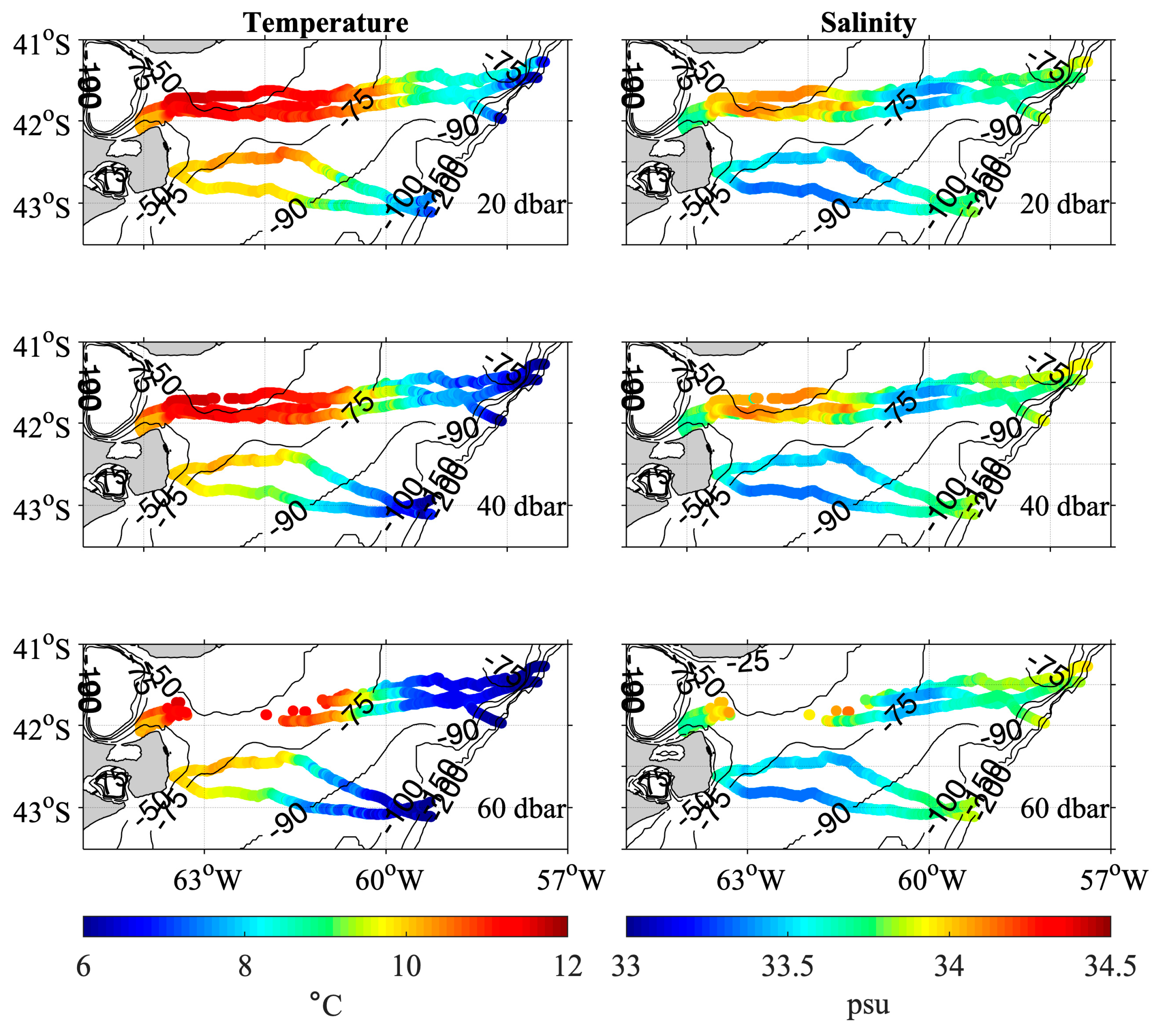
3.4. Analysis of the Temperature and Salinity Spatial Distributions

The spatial distribution of the temperature along the trajectories displays a zonal gradient, observing warm (warmer than 11 °C) water in the inner shelf and cold (colder than 6 °C) water in the outer shelf (Figure 6, left column). This is in good agreement with similar in-situ observations presented by Campagna et al. [11]. The zonal temperature gradient is evident in the three pressure levels (Figure 6, left column). The cold water close to the shelfbreak is associated with MC waters. A meridional gradient in the inner and middle shelves is also evident, showing that, north of 42°S, the surface temperature is 1 °C warmer than in the south (Figure 6).
In the northern trajectories, a maximum salinity (34 < S < 34.2) is observed when the depth is less than 60 m (Figure 6, right column). This region also has the warmest water (~12 °C). Near the 75 m isobath, the salinity decreases by 1 unit (S = 33.3) and increases again until it reaches 33.9 on the outer shelf. The temperature and salinity observed north of 42°S and west of the 75 m isobath are likely due to the mixing with waters coming from the SMG. The 75 m isobath coincides with the limit between the colder and fresher water from the south that moves towards the outer portion of the continental shelf and the hotter and saltier water closer to the coast, north of 42°S. The influence of the SMG waters over the adjacent portion of the continental shelf is in good agreement with previous observations [27].
Along the southern trajectories (south of 42°S), the salinity increases from 33.2 near the coast to 33.9 at the shelf-break in the three depth layers displayed (Figure 6).
Figure 6 also shows different values at the different depths in the temperature record, particularly in the mid and outer shelf, suggesting that waters are more stratified in those regions than in the inner shelf. Considering the large tidal amplitude in the region (Figure 3), we computed the Simpson parameter [58] to quantify in which regions tides are responsible for mixing waters and preventing seasonal stratification. We estimated the Simpson parameter (ϕ) as in Kahl et al. [59] using the in-situ data collected by the SESs. The spatial distribution of ϕ displays low values (<10 J/m3) in the inner shelf and larger values (10–50 J/m3) in the middle and outer shelves (not shown). The most significant ϕ (critical value of 10 J/m3) occurs along the 75 m isobath, suggesting that well-mixed waters are located between such isobath and the coast and stratified waters are in waters deeper than 75 m. This result is in very good agreement with our observations in the following sections. In this study region, Lucas et al. [27] and Kahl et al. [59] showed the spatial distribution of ϕ for spring/summer with a critical value of 40–50 J/m3 that followed the 50–60 m isobath. The values obtained in this work are low because October is a transition period toward strong stratification due to the solar radiation annual cycle. A similar result was found between 47° and 55°S in October 2005 by Sabatini et al. [60].

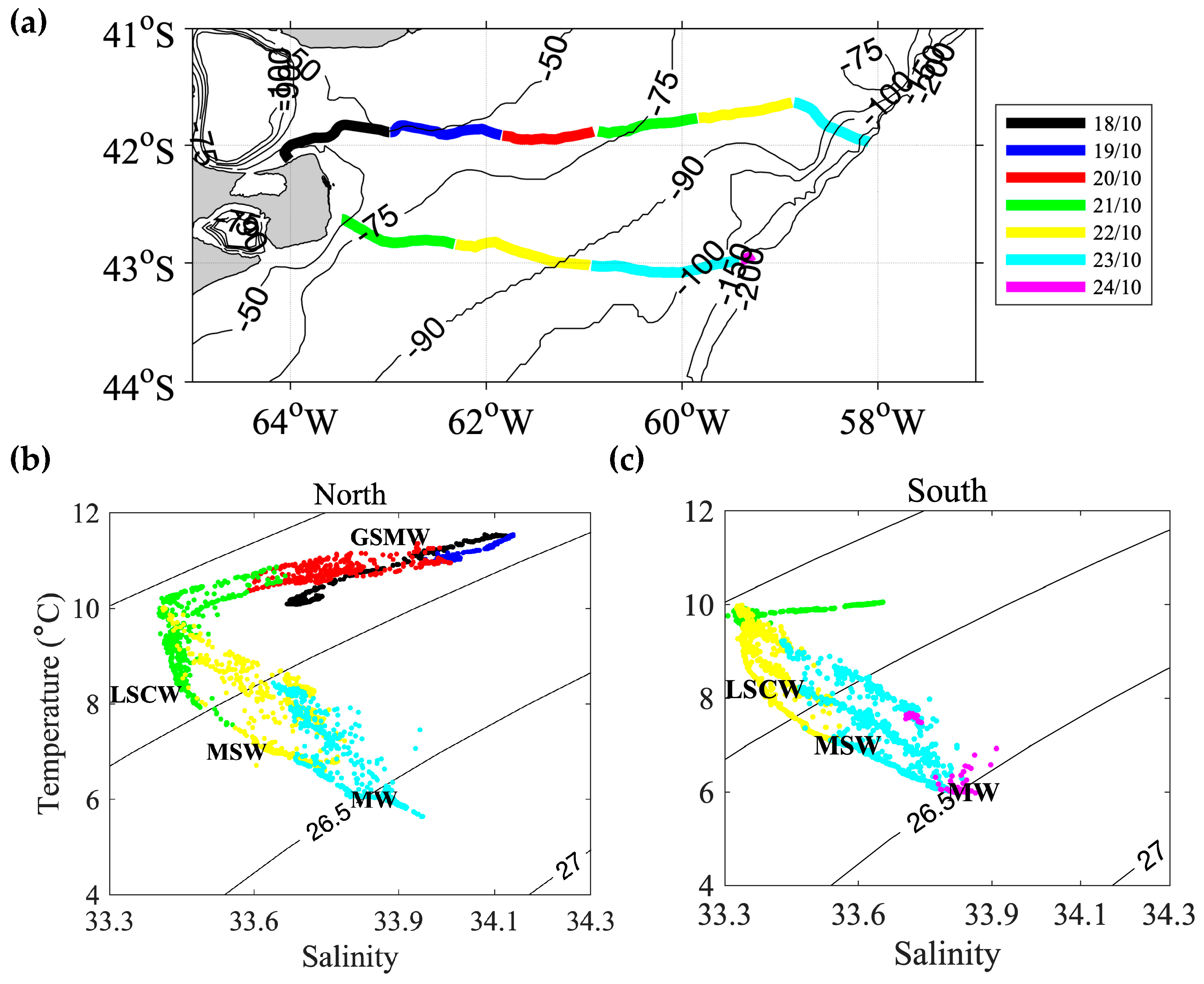
3.5. Water Mass Characterization

In Section 3.4, we showed that the data collected in the northern trajectories differs quite a bit from the data collected in the southern trajectories. In what follows, we analyze the water masses north and south of 42°S, selecting one representative trajectory for each region. We used trajectory 051 to represent the southern ones and 875 for the northern ones (Figure 1).
Both Northern and Southern SESs swam across three distinctive water masses that were identified in the TS diagrams: Low Salinity Coastal Waters (LSCW, S < 33.4), Mid-Shelf Waters (MSW, 33.4 < S < 33.8), and Malvinas Waters (MW, S > 33.8) (Figure 7b,c). The Northern elephant also crossed the High Salinity Coastal Waters (HSCW, S > 34) at the beginning of its trip (18, 19, and 20 of October), which contain waters from SMG (Figure 7b). SMG has higher temperatures and salinity values relative to the continental shelf because it is an evaporation basin, i.e., precipitation is lower than evaporation [28,61,62]. As described above, the waters adjacent to the SMG are affected by the waters from the gulf. The HSCW is not present south of 42°S.
The LSCW and MSW were sampled by the southern and northern SESs on the 22 and 23 of October (Figure 7). These water masses originate in the coastal Pacific Ocean and are transported by the Patagonian current [63].

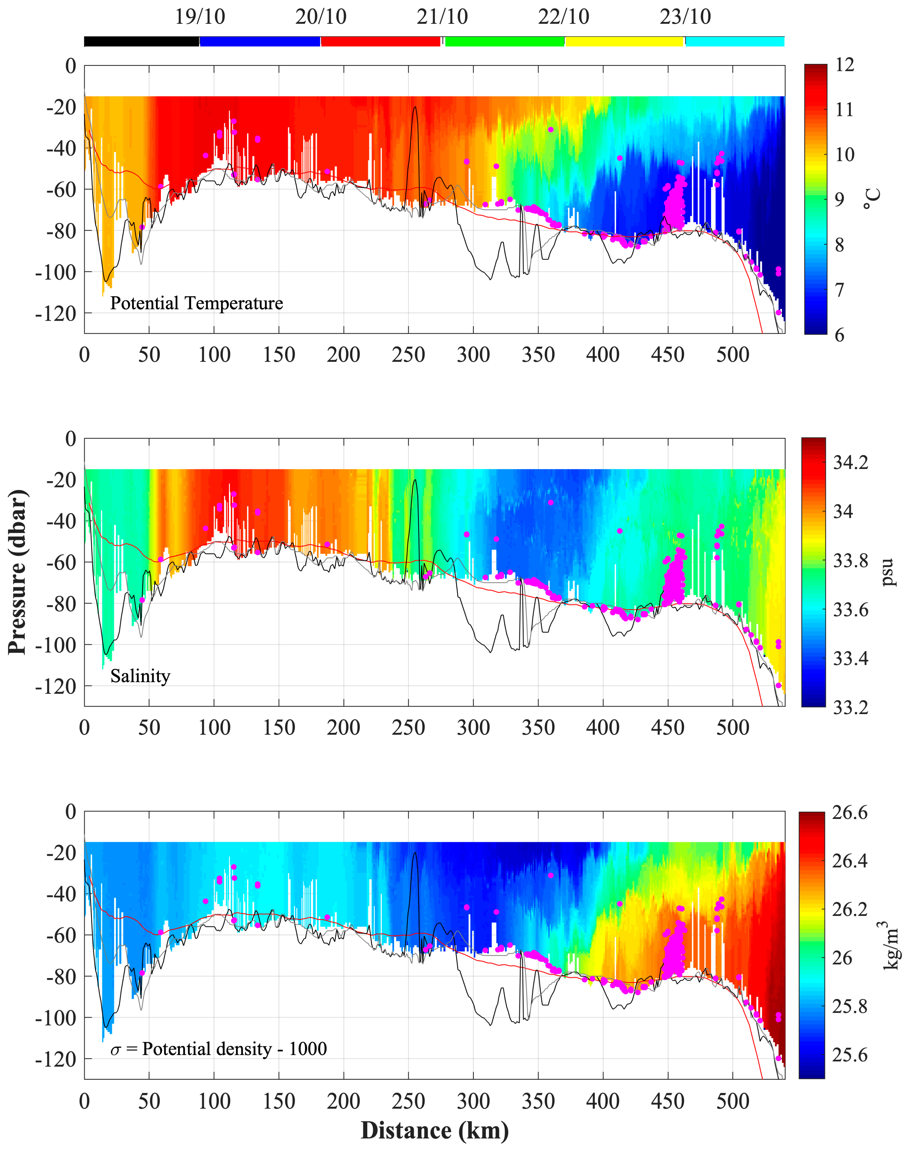
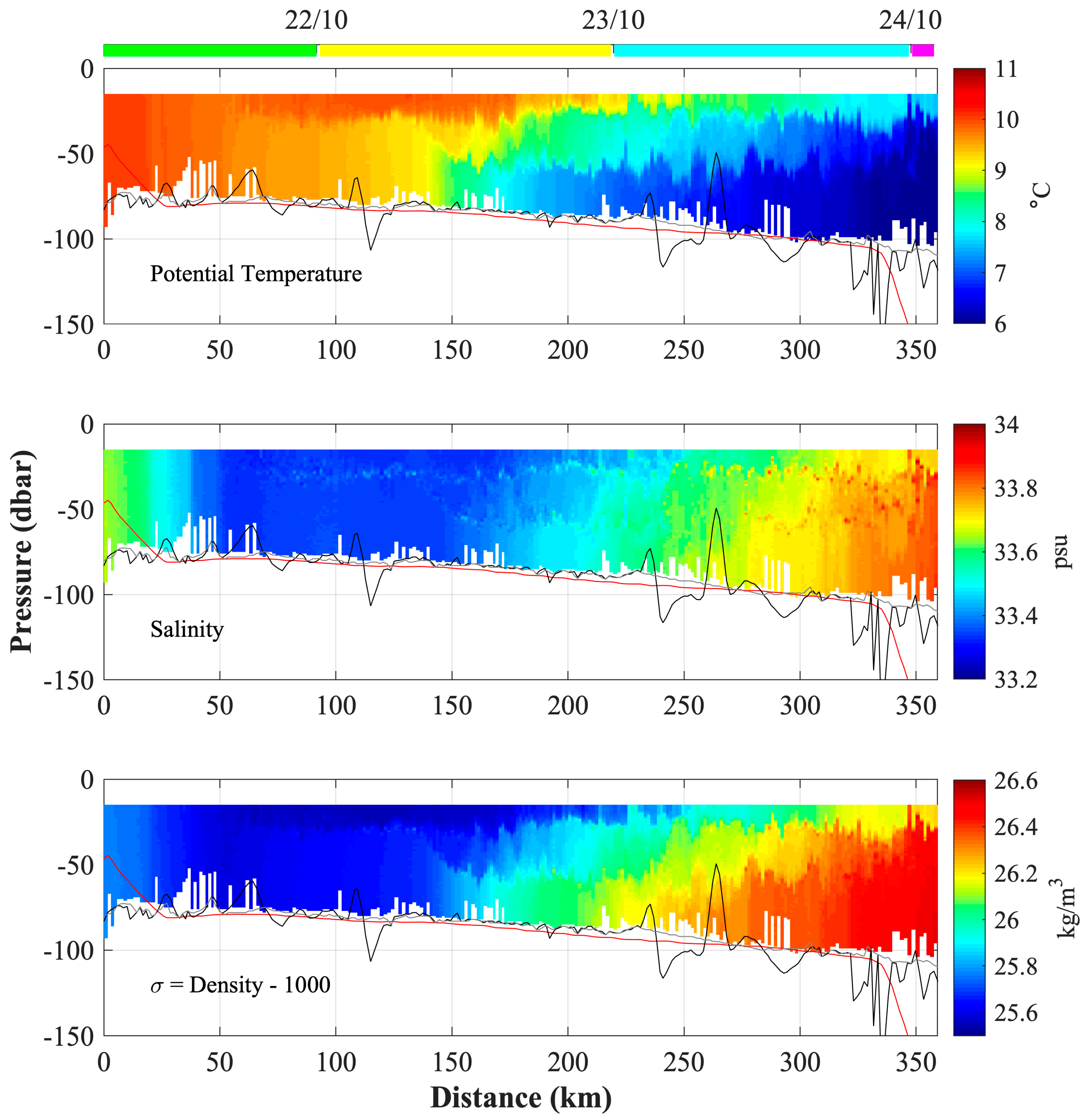
3.6. Vertical Profiles of Temperature, Salinity, and Density

3.6.1. Northern Trajectory

The northern elephant had 479 profiles, with an average distance between each profile of 1.1 km and an average profile depth of 67.3 m.
The vertical structure of the temperature is homogeneous from the surface to the bottom in the first 300 km from the coast (Figure 8, upper panel). During the first day after departure from the north of PV (19 October 2019), the potential temperature profile displays several increases and decreases in temperature (between 10 °C and 11 °C). From km 300 towards the shelf break, a vertical stratification begins, which is accentuated towards the slope with temperatures of 8 °C on the surface and 6 °C on the bottom (Figure 8 upper panel).
The vertical salinity structure along the trajectory also presents an oscillating pattern during the first day after departure, with salinity values between 33.6 and 34. Between 300 and 400 km from the coast, on the middle continental shelf, the salinity shows minimal values of 33.4 from surface to bottom. Then, the salinity increases towards the east, reaching values of 33.6–33.9 (Figure 8 middle panel).
The vertical density structure depends on temperature and salinity; homogeneous values are observed from surface to bottom and from the coast up to about 320 km (Figure 8 bottom panel). The spatial density distribution also shows the strip pattern identified in temperature and salinity during 19th of October. In the middle continental shelf (~350 km), a density minimum modulated mainly by salinity is observed. From 400 km to the edge of the shelf, the density is dominated by T and S. In this section, a weak vertical stratification begins, which increases towards the slope. An increase in salinity (33.6 < S < 33.9) and a decrease in temperature (<8 °C) in the bottom are observed in this portion of the section in Figure 8 (upper and middle panels), clearly suggesting intrusions of the saltier and colder MC water. Such intrusions have been previously reported at 41°S by Piola et al. [19].
PCA values are indicated with magenta dots in the three panels of Figure 8. A few values are observed at the sea bottom along the section. A large concentration of PCAs is observed in a particular region on the outer shelf, between 450 and 480 km from the coast. A careful inspection of the T and S values shows an increase in salinity in this region, which coincides with a decrease in temperature of 0.5 °C and an increase in density (from 26.3 to 26.4 kg/m3). As discussed above, this water mass can only originate from an intrusion of the MC. It is very interesting to note the correspondence between the large number of PCAs and the T and S values that most closely resemble the MC waters. The fact that many PCAs are observed in a particular region where the MC rested isolated suggests that the MC waters bring food the SESs like.
The analysis of Figure 8 in conjunction with the analysis of the spatial distribution of T and S (Section 3.4) and the TS diagrams (Section 3.5) allows us to identify that the warm and salty region (between km 80 and km 250, Figure 8) corresponds to the HSCW from SMG. The strip pattern observed in T and S the first day after its departure indicates that the SES swam across different water masses at the beginning of its trip. To further understand these features, we used satellite SST images that showed excellent agreement with the in-situ data (Section 3.3). On the 18th of October 2019, SST agreed to an alternating pattern of increasing and decreasing values (Figure 9a) that agreed with the pattern observed in Figure 8. The spatial pattern of SST indicates that the relative cold water is advected from the south into the SMG and that the relative warm water corresponds to HSCW. Moreover, the monthly average of 17 years of SST gradient reveals that in October there is a strong and persistent front (0.06 °C/km) at 41.9°S and between 63.3° and 63.6°W (Figure 9b). The front separates warm and salty water from SMG and cold and fresh water from the southern portion of the adjacent shelf. The Northern SES crossed this frontal area, explaining the abrupt temperature changes observed in Figure 8. Figure 9 also indicates that the other two northern SESs crossed the frontal area. The frontal area north of PV has been reported in Pisoni [64]. Using SST satellite images, they show that it is a seasonal front that exists during winter and the beginning of spring. The TS values recorded by the SESs in conjunction with SST images show that the front separates fresh and cold waters that enter the SMG in the narrow region between the coast and the front from warm and salty water created in the SMG, north of the front. The water entering the SMG comes from the coastal region east of PV, where a strong upwelling took place [26].

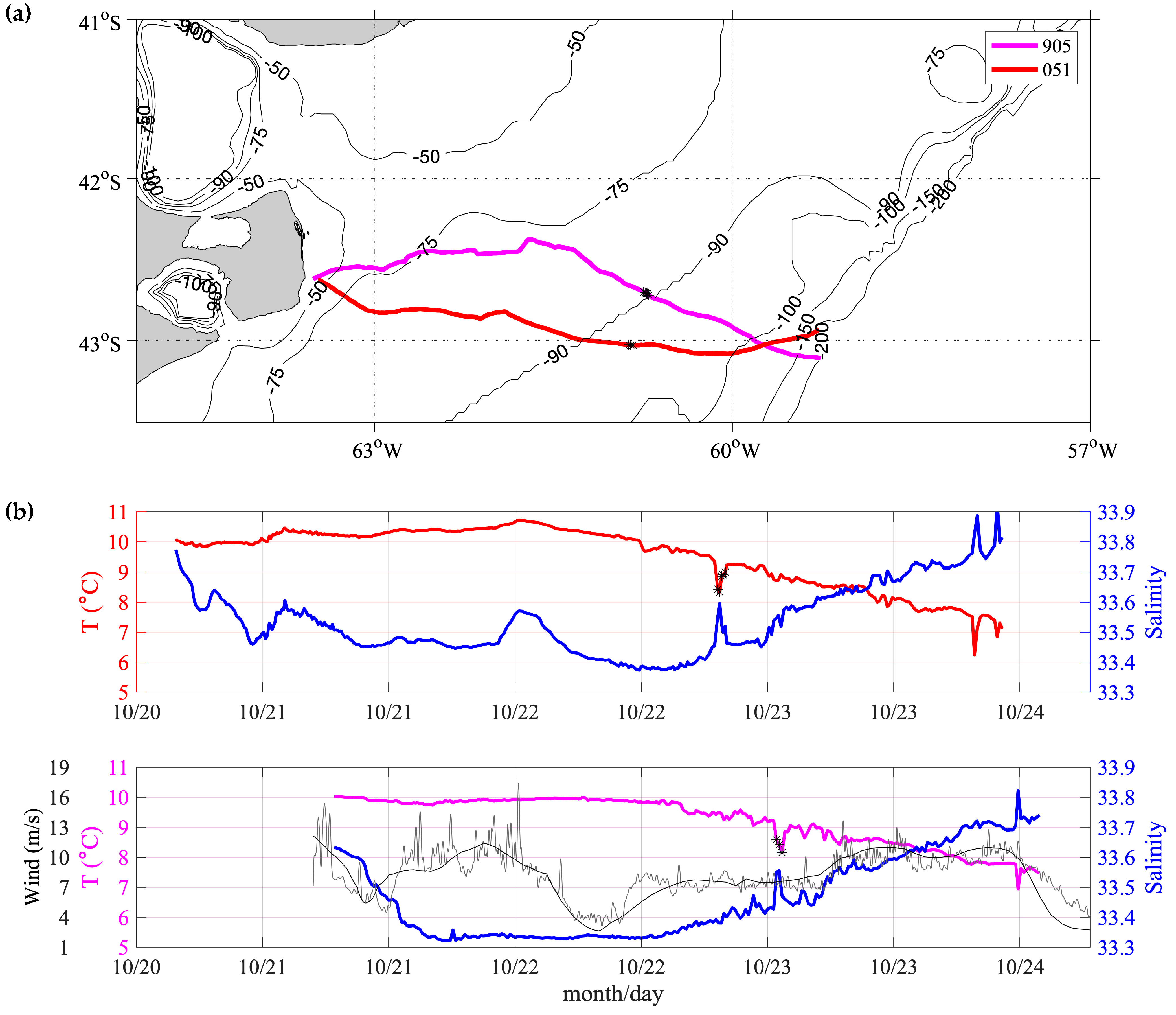
3.6.2. Southern Trajectory

Potential temperature, salinity, and potential density for the Southern elephant seal are presented in Figure 10. The southern elephant conducted 259 profiles, with an average distance between each profile of 1.4 km and an average profile depth of 82.8 m. The temperature shows homogeneous values in the vertical of about 10 °C in the first 50 km of the trajectory. Warmer values in the upper 30 m of the water column are observed from km 50 to the shelf-break, suggesting the presence of seasonal stratification (Figure 10 upper panel). Cold waters (less than 8 °C) are observed close to the sea floor from km 180 towards the edge of the shelf-break (Figure 10), as observed in the northern trajectory.
Salinity along the southern trajectory (Figure 10 middle panel) is vertically homogeneous in the first 180 km, with relative salty values close to the coast (33.6) that decrease up to 33.3 in the east. The lowest salinity values (33.3) occupy a large portion of the section, from 50 to 180 km from the shore. These values are characteristic of the diluted water coming from the Chilean coast through the Magellan Strait. From km 180 to the shelf-break, the salinity increases to 33.8.
The density section (Figure 10, bottom panel) shows homogeneous values in the vertical range of 25.7 kg/m3 in the first 50 km of the trajectory. The density pattern is similar to the salinity pattern between 0 and 150 km from the shore, suggesting that density is dominated by S. Between 150 km and the shelf break, a comparison of the three panels of Figure 10 indicates that the density is dominated by the contributions of both T and S. The cold and salty waters (T < 7 °C and S > 33.8) occupy most of the mid and outer shelf in the deepest portion of the water column between 180 km and the shelf break. These values are due to the mixing between MW and MSW.
A particular feature is observed in three consecutive temperature profiles of the Southern elephant, between 15 and 35 dbar at ~225 km from the coast (Figure 10 top panel). To better study this event, we plotted the potential temperature and salinity at 15 dbar for all the SESs. The cooling event detected by SES 051 was also detected in SES 905, with a time difference of 6 h (Figure 11). The potential temperature drop of 1 °C in both SESs was accompanied by an increase in salinity of ~0.2 psu (Figure 11).
Similar cooling events have been observed in the ACS and have been attributed to strong winds and/or rapid changes in the wind stress direction, generally due to the passage of a low-pressure system [49]. Such low-pressure systems intensify the sea surface wind and temporarily disrupt vertical stratification. The sea level pressure analysis provided by ERA5 (ECMWF Reanalysis v5) shows that a low-pressure system over the shelf coincided in time and space with the anomalies along the SESs 905 and 051 discussed here (Figure 11). Yet, wind estimation from ERA5 does not show an abrupt change in the wind stress intensity at the time when the anomalies were observed on the 22 and 23 of October 2019 (Figure 11). Figure 11b also shows an excellent correlation (r = 0.81, significant at the 95% confidence level (CL95%)) between the DTAG-4 wind estimates and ERA5, further supporting the capacity of the DTAG-4 logger to estimate wind and providing confidence in the ERA5 wind data [65].
We therefore conclude that local wind was not responsible for disrupting the stratification of the water column observed on the 22 and 23 of October 2019. The disruption of the stratification could also be due to the passage of internal waves, a possibility that we will investigate in future work.

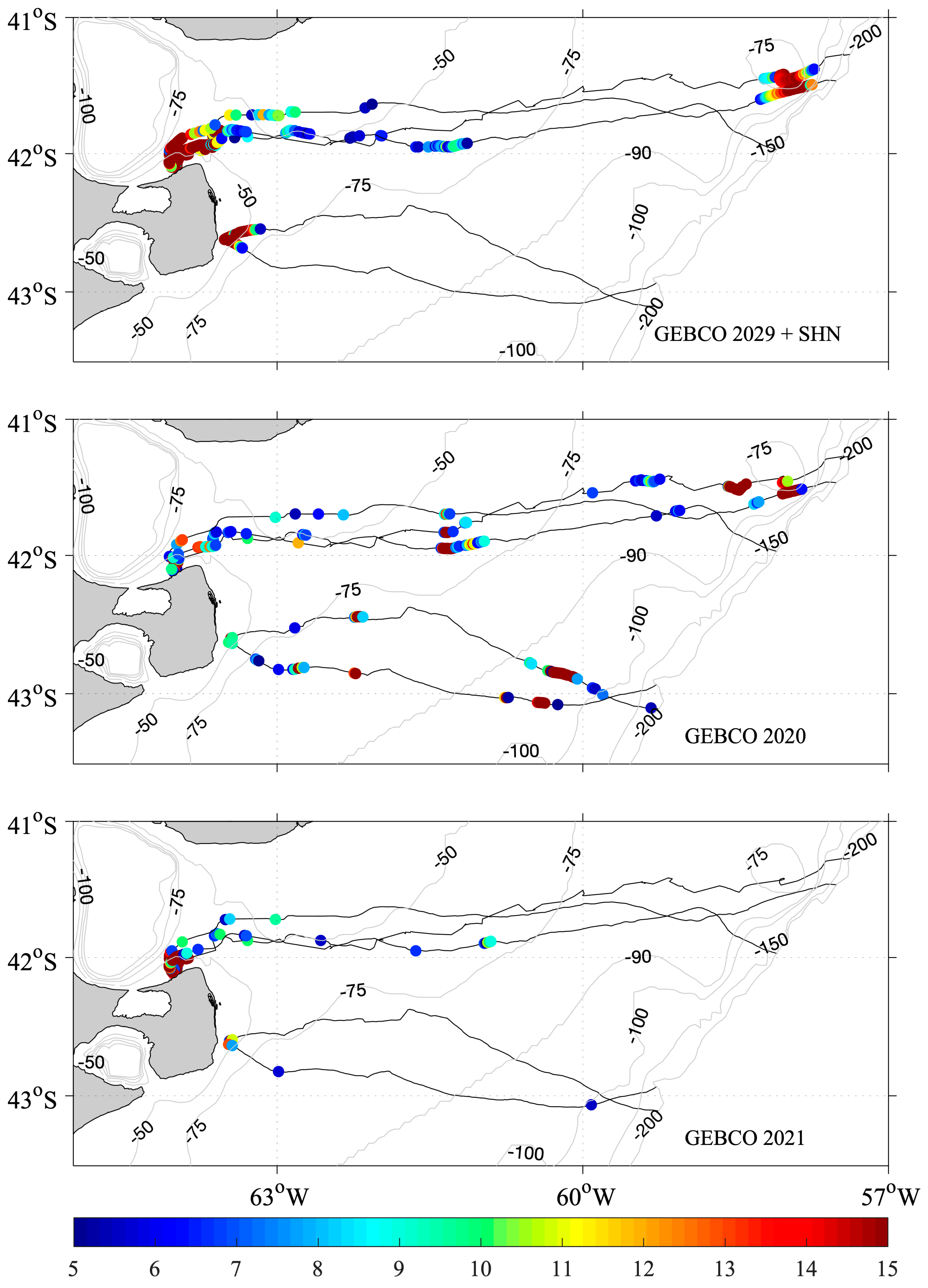
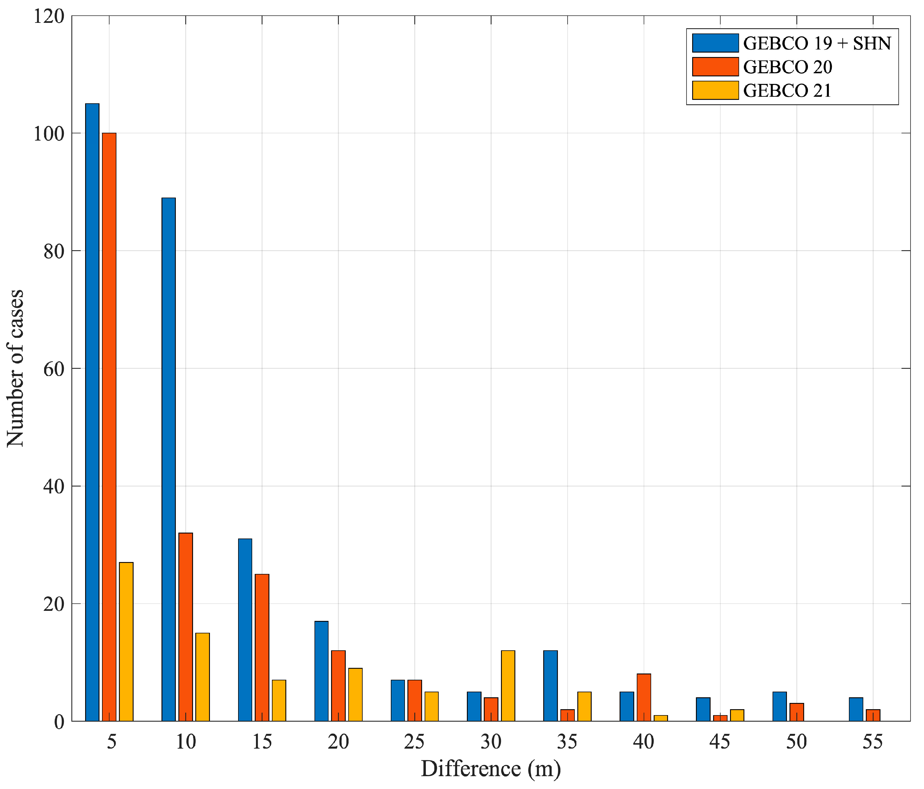
3.7. Comparison between Depths Reached by SESs and GEBCO Bathymetric Charts

The maximum depth reached by the SESs is higher than reported in bathymetric charts from GEBCO (2019 + SHN, 2020, and 2021) along several portions of the trajectories (Figure 8 and Figure 10). Thus, the depths reached by the SESs may be a useful variable to calibrate/validate the bathymetric charts. Here, a quantitative comparison is presented between the maximum depth reached by SESs and the corresponding value provided by bathymetric charts (Figure 10). Note that we neglected the cases where the depth reached by the SESs was lower than the GEBCO products since we cannot guarantee that the SESs reached the sea floor. Most of the discrepancies are observed near the coast for the three datasets, especially in the northern trajectories, reaching values larger than 10 m (Figure 12). The lowest bias values (< 9 m) are observed on the middle shelf for GEBCO 2019 + SHN and GEBCO 2021. GEBCO 2019 + SHN underestimates the depth on the outer shelf with values larger than 12 m. Figure 12 also revealed that GEBCO 2020 undervalues the depth throughout the trajectories. The histogram of the bathymetry differences higher than 5 m (Figure 13) confirms that GEBCO 2021 is the bathymetry chart that presented the lowest number of cases where the depth reached by SESs is higher, suggesting that it is the best option available to represent the bathymetry in the region.

4. Summary and Discussion

In this study, we analyzed high-spatial and temporal-resolution hydrographic data collected by five SESs that crossed the ACS between 44°S and 41°S in October 2019.
The spatial distribution of temperature and salinity revealed two regions, north and south of 42°S. The northern region is 1 °C warmer and 0.5 psu saltier than the southern region due to the fact that in the latter, the diluted water coming from the south mixes with the High-Salinity Coastal Water coming from SMG.
The spatial patterns of T and S at different pressure levels also indicated that the 75 m isobath delimited the vertically homogeneous region from the stratified one. Indeed, the 75 m isobath corresponds with the position of the largest increment of the Simpson parameter computed along the SESs trajectories. The Simpson parameter at the 75 m isobath is 10 J/m3, a rather low value compared with values commonly found in the region to separate coastal mixed waters from open ocean stratified waters [27,59,66]. This is probably due to the fact that our estimation of the Simpson parameter has been conducted in austral spring (mid-October), a period of the year when the vertical stratification over the continental shelf is much lower than in austral summer, when the other estimations have been conducted [24,66].
SST from MUR correlates very well (r = 0.97) with the T measured at 15 m depth by SESs. Both datasets show the presence of an advective front in the northern region of PV, between 63.3°W and 63.6°W, at 41.9°S. Pisoni [64] described such a front using only satellite SST data and discussed that an intense coastal jet carries cold and fresh waters from the western coast of PV, causing the formation of the so-called advective front. T and S data provided by the three SESs that sampled the waters on both sides of the front allowed showing that there is a gradient of salinity also in the region.
The SESs crossed the ACS in a few days with a mean speed of 1–1.5 m/s, similar to the values documented by Campagna et al. [11] and one order of magnitude higher than the geostrophic velocities in the area [49]. We show for the first time that SESs speed might be modulated by tidal currents: the speed of the three northern SESs showed a semi-diurnal cycle that correlates with the macro-tidal regime observed close to the coast, north of 42°S. South of 42°S, this oscillation is not observed since the tidal velocities are not as large as in the northern region.
Temperature and salinity along the trajectories might present large variations (Figure 11). Local wind stress estimated from an acoustic sensor mounted on some of the SESs and as computed by ERA5 reanalysis data does not show large values related to T and S abrupt changes observed. We argue that the passage of internal waves originating in a remote place could be the force that explains the anomalies observed.
PCA values suggest that SESs feed mostly at the bottom of the sea when crossing the ACS. Only SES 875 fed intensively in a particular region located on the outer shelf, between 50 m and the sea bottom, located at 80 m. The T and S analyses showed that such a region was occupied by an intrusion of MC waters. We suggest that MC carried prey that SES 875 liked.
Lastly, the records of the maximum depth reached by the SESs provide valuable information to calibrate/validate bathymetric charts. Our results pointed out the regions along the trajectories where the bathymetry from three GEBCO products underestimated the depth of the sea. A reliable topography is crucial for ocean numerical models to reproduce a realistic circulation [67].
The SES colony of PV has been demonstrated to be an excellent platform for measuring oceanographic variables at high spatial and temporal resolution over the ACS, providing an average of 92.6 dives per day and one profile every 1.1km. This unique dataset opens the opportunity to explore physical, small-scale processes that are not yet well understood but can have a significant impact on the air-sea fluxes of CO2 and heat advection. The continuity of high-frequency, high-spatial-resolution hydrographic data are crucial for studying these processes and their variability. Hence, maintaining the deployment and collection of data collected through SESs could enhance the comprehension of the climate change process in the region. Variations in temperatures, currents, and salinity can deeply impact marine ecosystems, biodiversity, and biological productivity [33,68]. Finally, this work highlights the advantages of the utilization of mammal-based sensors in comparison to gliders and Argo floats. Many of the regions sampled by the SESs in the ACS are shallow (less than 50 m) and are characterized by strong tidal currents (up to 2.5 m/s), largely limiting the operability of gliders and Argo floats. The mammal-based sensors, through their unique capabilities, allow more effective data collection under such conditions.

Author Contributions

Conceptualization, L.A.R.-E. and M.S.; Methodology, M.M.M., L.A.R.-E. and M.S.; Software, M.M.M.; Validation, M.M.M., A.G.-M., B.P. and C.G.; Formal analysis, M.M.M.; Investigation, M.M.M., L.A.R.-E. and M.S.; Resources, M.S. and C.G.; Data curation, B.P.; Writing—original draft, M.M.M.; Writing—review & editing, M.M.M., L.A.R.-E., M.S., A.G.-M., J.C., B.P. and C.G.; Visualization, M.M.M. and L.A.R.-E.; Supervision, M.S.; Project administration, M.S. All authors have read and agreed to the published version of this manuscript.

Funding

This research was funded by European Organization for the Exploitation of Meteorological Satellites (EUMETSAT)/ Centre National de la Recherche Spatial (CNES) through Project Studying physical processes in the Southwestern Atlantic to understand BIOlogical productivity & regional Ecosystems (SABIO) and Wildlife Conservation Society (WCS).

Data Availability Statement

The marine mammal data were collected and made freely available by the International MEOP Consortium and the national programs that contribute to it. (http://www.meop.net, accessed on 3 May 2021).

Acknowledgments

We are grateful to all the field personnel that assisted in the deployment and recoveries of data loggers: Claudio Campagna, Loic Le Ster, Mark Hindell and Ricardo Vera. We also thank the institutions that provided additional support: Mincyt Pampa Azul Project B6 and PICT 2020-SERIEA-01468. The manuscript was improved by comments from the four anonymous reviewers.

Conflicts of Interest

The authors declare no conflict of interest.

References

  1. Harcourt, R.; Sequeira, A.M.M.; Zhang, X.; Roquet, F.; Komatsu, K.; Heupel, M.; McMahon, C.; Whoriskey, F.; Meekan, M.; Carroll, G.; et al. Animal-Borne Telemetry: An Integral Component of the Ocean Observing Toolkit. Front. Mar. Sci. 2019, 6, 326. [Google Scholar] [CrossRef]
  2. Chapman, C.C.; Lea, M.-A.; Meyer, A.; Sallée, J.-B.; Hindell, M. Defining Southern Ocean fronts and their influence on biological and physical processes in a changing climate. Nat. Clim. Chang. 2020, 10, 209–219. [Google Scholar] [CrossRef]
  3. Treasure, A.M.; Roquet, F.; Ansorge, I.J.; Bester, M.N.; Boehme, L.; Bornemann, H.; Charrassin, J.-B.; Chevallier, D.; Costa, D.P.; Fedak, M.A.; et al. Marine Mammals Exploring the Oceans Pole to Pole: A Review of the MEOP Consortium. Oceanography 2017, 30, 132–138. [Google Scholar] [CrossRef]
  4. McIntyre, T.; de Bruyn, P.J.N.; Ansorge, I.J.; Bester, M.N.; Bornemann, H.; Plötz, J.; Tosh, C.A. A lifetime at depth: Vertical distribution of southern elephant seals in the water column. Polar Biol. 2010, 33, 1037–1048. [Google Scholar] [CrossRef]
  5. Boehme, L.; Lovell, P.; Biuw, M.; Roquet, F.; Nicholson, J.; Thorpe, S.E.; Meredith, M.P.; Fedak, M. Technical Note: Animal-borne CTD-Satellite Relay Data Loggers for real-time oceanographic data collection. Ocean Sci. 2009, 5, 685–695. Available online: www.ocean-sci.net/5/685/2009/ (accessed on 30 June 2021). [CrossRef]
  6. Roquet, F.; Park, Y.-H.; Guinet, C.; Bailleul, F.; Charrassin, J.-B. Observations of the Fawn Trough Current over the Kerguelen Plateau from instrumented elephant seals. J. Mar. Syst. 2009, 78, 377–393. [Google Scholar] [CrossRef]
  7. Hindell, M.A.; McMahon, C.R.; Jonsen, I.; Harcourt, R.; Arce, F.; Guinet, C. Inter- and intrasex habitat partitioning in the highly dimorphic southern elephant seal. Ecol. Evol. 2021, 11, 1620–1633. [Google Scholar] [CrossRef]
  8. Bailleul, F.; Charrassin, J.-B.; Monestiez, P.; Roquet, F.; Biuw, M.; Guinet, C. Successful foraging zones of southern elephant seals from the Kerguelen Islands in relation to oceanographic conditions. Philos. Trans. R. Soc. B Biol. Sci. 2007, 362, 2169–2181. [Google Scholar] [CrossRef]
  9. Dragon, A.-C.; Monestiez, P.; Bar-Hen, A.; Guinet, C. Linking foraging behaviour to physical oceanographic structures: Southern elephant seals and mesoscale eddies east of Kerguelen Islands. Prog. Oceanogr. 2010, 87, 61–71. [Google Scholar] [CrossRef]
  10. Hindell, M.A.; McMahon, C.R.; Bester, M.N.; Boehme, L.; Costa, D.; Fedak, M.A.; Guinet, C.; Herraiz-Borreguero, L.; Harcourt, R.G.; Huckstadt, L.; et al. Circumpolar habitat use in the southern elephant seal: Implications for foraging success and population trajectories. Ecosphere 2016, 7, e01213. [Google Scholar] [CrossRef]
  11. Campagna, C.; Piola, A.R.; Marin, M.R.; Lewis, M.; Fernández, T. Southern elephant seal trajectories, fronts and eddies in the Brazil/Malvinas Confluence. Deep Sea Res. Part I Oceanogr. Res. Pap. 2006, 53, 1907–1924. [Google Scholar] [CrossRef]
  12. Campagna, J.; Lewis, M.N.; González Carman, V.; Campagna, C.; Guinet, C.; Johnson, M.; Randall WDavis Rodríguez, D.H.; Hindell, M.A. Ontogenetic niche partitioning in southern elephant seals from Argentine Patagonia. Mar. Mammal Sci. 2020, 37, 631–651. [Google Scholar] [CrossRef]
  13. Aubone, N.; Saraceno, M.; Alberto, M.T.; Campagna, J.; Le Ster, L.; Picard, B.; Hindell, M.; Campagna, C.; Guinet, C. Physical changes recorded by a deep diving seal on the Patagonian slope drive large ecological changes. J. Mar. Syst. 2021, 223, 103612. [Google Scholar] [CrossRef]
  14. Campagna, C.; LE Boeuf, B.J.; Blackwell, S.B.; Crocker, D.E.; Quintana, F. Diving behaviour and foraging location of female southern elephant seals from Patagonia. J. Zool. 1995, 236, 55–71. [Google Scholar] [CrossRef]
  15. McGovern, K.; Rodríguez, D.; Lewis, M.; Eder, E.; Piola, A.; Davis, R. Habitat associations of post-breeding female southern elephant seals (Mirounga leonina) from Península Valdés, Argentina. Deep Sea Res. Part I Oceanogr. Res. Pap. 2022, 185, 103789. [Google Scholar] [CrossRef]
  16. Campagna, C.; Lewis, M. Growth and Distribution of A Southern Elephant Seal Colony. Mar. Mammal Sci. 1992, 8, 387–396. [Google Scholar] [CrossRef]
  17. Laws, R.M. History and present status of southern elephant seal populations. In Elephant Seals: Population ecology, Behavior and Physiology; Le Boeuf, B.J., Laws, R.M., Eds.; University of California Press: Berkeley, CA, USA, 1994; pp. 49–65. [Google Scholar]
  18. Campagna, C.; Piola, A.R.; Marin, M.R.; Lewis, M.; Zajaczkovski, U.; Fernández, T. Deep divers in shallow seas: Southern elephant seals on the Patagonian shelf. Deep Sea Res. Part I Oceanogr. Res. Pap. 2007, 54, 1792–1814. [Google Scholar] [CrossRef]
  19. Piola, A.R.; Avellaneda, N.M.; Guerrero, R.A.; Jardón, F.P.; Palma, E.D.; Romero, S.I. Malvinas-slope water intrusions on the northern Patagonia continental shelf. Ocean Sci. 2010, 6, 345–359. [Google Scholar] [CrossRef]
  20. Glorioso, P.D. Temperature distribution related to shelf-sea fronts on the Patagonian Shelf. Cont. Shelf Res. 1987, 7, 27–34. [Google Scholar] [CrossRef]
  21. Sabatini, M.; Martos, P. SCIENTIA MARINA Mesozooplankton features in a frontal area off northern Patagonia (Argentina) during spring 1995 and 1998. Sci. Mar. 1995, 66, 215–232. [Google Scholar] [CrossRef]
  22. Romero, S.I.; Piola, A.R.; Charo, M.; Garcia, C.A.E. Chlorophyll-a variability off Patagonia based on SeaWiFS data. J. Geophys. Res. Ocean 2006, 111. [Google Scholar] [CrossRef]
  23. Rivas, A.L.; Pisoni, J.P. Identification, characteristics and seasonal evolution of surface thermal fronts in the Argentinean Continental Shelf. J. Mar. Syst. 2010, 79, 134–143. [Google Scholar] [CrossRef]
  24. Bogazzi, E.; Baldoni, A.; Rivas, A.; Martos, P.; Reta, R.; Orensanz, J.M.; Lasta, M.; Dell’Arciprete, P.; Werner, F. Spatial correspondence between areas of concentration of Patagonian scallop (Zygochlamys patagonica) and frontal systems in the southwestern Atlantic. Fish. Oceanogr. 2005, 14, 359–376. [Google Scholar] [CrossRef]
  25. Franco, B.C.; Palma, E.D.; Tonini, M.H. Benthic-pelagic uncoupling between the Northern Patagonian Frontal System and Patagonian scallop beds. Estuar. Coast. Shelf Sci. 2015, 153, 145–155. [Google Scholar] [CrossRef]
  26. Tonini, M.H.; Palma, E.D.; Pisoni, J.P. Modeling the seasonal circulation and connectivity in the North Patagonian Gulfs, Argentina. Estuar. Coast. Shelf Sci. 2022, 271, 107868. [Google Scholar] [CrossRef]
  27. Lucas, A.J.; Guerrero, R.A.; Mianzán, H.W.; Acha, E.M.; Lasta, C.A. Coastal oceanographic regimes of the Northern Argentine Continental Shelf (34–43°S). Estuar. Coast. Shelf Sci. 2005, 65, 405–420. [Google Scholar] [CrossRef]
  28. Piola, A.R.; Scasso, L.M. Circulación en el golfo San Matías. Geoacta 1988, 15, 33–51. [Google Scholar]
  29. Bianchi, A.A.; Bianucci, L.; Piola, A.R.; Pino, D.R.; Schloss, I.; Poisson, A.; Balestrini, C.F. Vertical stratification and air-sea CO2 fluxes in the Patagonian shelf. J. Geophys. Res. Ocean 2005, 110, 1–10. [Google Scholar] [CrossRef]
  30. Lusquiños, A.J.; Valdés, A.J. Aportes al Conocimiento de las Masas de Agua del Atlántico Sudoccidental; Rep. H659; Serv. de Hidrografía Nav.: Buenos Aires, Argentina, 1971; p. 48. [Google Scholar]
  31. Saraceno, M.; Martín, J.; Moreira, D.; Pisoni, J.P.; Tonini, M.H. Physical Changes in the Patagonian Shelf. In Global Change in Atlantic Coastal Patagonian Ecosystems: A Journey Through Time; Helbling, E.W., Narvarte, M.A., González, R.A., Villafañe, V.E., Eds.; Springer International Publishing: Berlin/Heidelberg, Germany, 2022; pp. 43–71. [Google Scholar] [CrossRef]
  32. Photopoulou, T.; Fedak, M.A.; Matthiopoulos, J.; McConnell, B.; Lovell, P. The generalized data management and collection protocol for Conductivity-Temperature-Depth Satellite Relay Data Loggers. Anim. Biotelemetry 2015, 3, 21. [Google Scholar] [CrossRef]
  33. Roquet, F.; Boehme, L.; Block, B.; Charrasin, J.B.; Costa, D.; Guinet, C.; Harcourt, R.G.; Hindell, M.A.; Hückstädt, L.A.; McMahon, C.R.; et al. Ocean Observations Using Tagged Animals. Oceanography 2017, 30, 139. [Google Scholar] [CrossRef]
  34. Goulet, P.; Guinet, C.; Swift, R.; Madsen, P.T.; Johnson, M. A miniature biomimetic sonar and movement tag to study the biotic environment and predator-prey interactions in aquatic animals. Deep Sea Res. Part I Oceanogr. Res. Pap. 2019, 148, 1–11. [Google Scholar] [CrossRef]
  35. Guinet, C.; Vacquié-Garcia, J.; Picard, B.; Bessigneul, G.; Lebras, Y.; Dragon, A.; Viviant, M.; Arnould, J.; Bailleul, F. Southern elephant seal foraging success in relation to temperature and light conditions: Insight into prey distribution. Mar. Ecol. Prog. Ser. 2014, 499, 285–301. [Google Scholar] [CrossRef]
  36. Vacquié-Garcia, J.; Guinet, C.; Laurent, C.; Bailleul, F. Delineation of the southern elephant seal’s main foraging environments defined by temperature and light conditions. Deep Sea Res. Part II Top. Stud. Oceanogr. 2015, 113, 145–153. [Google Scholar] [CrossRef]
  37. Merchant, N.D.; Fristrup, K.M.; Johnson, M.P.; Tyack, P.L.; Witt, M.J.; Blondel, P.; Parks, S.E. Measuring acoustic habitats. Methods Ecol. Evol. 2015, 6, 257–265. [Google Scholar] [CrossRef] [PubMed]
  38. Lopez, R.; Malardé, J.-P.; Danès, P.; Gaspar, P. Improving Argos Doppler location using multiple-model smoothing. Anim. Biotelemetry 2015, 3, 32. [Google Scholar] [CrossRef]
  39. Dragon, A.-C.; Bar-Hen, A.; Monestiez, P.; Guinet, C. Horizontal and vertical movements as predictors of foraging success in a marine predator. Mar. Ecol. Prog. Ser. 2012, 447, 243–257. [Google Scholar] [CrossRef]
  40. Lowther, A.D.; Lydersen, C.; Fedak, M.A.; Lovell, P.; Kovacs, K.M. The Argos-CLS Kalman Filter: Error Structures and State-Space Modelling Relative to Fastloc GPS Data. PLoS ONE 2015, 10, e0124754. [Google Scholar] [CrossRef] [PubMed]
  41. Ryan, P.G.; Petersen, S.L.; Peters, G. GPS tracking a marine predator: The effects of precision, resolution and sampling rate on foraging tracks of African Penguins. Mar. Biol. 2004, 145, 215–223. [Google Scholar] [CrossRef]
  42. Le Bras, Y.; Jouma’a, J.; Picard, B.; Guinet, C. How Elephant Seals (Mirounga leonina) Adjust Their Fine Scale Horizontal Movement and Diving Behaviour in Relation to Prey Encounter Rate. PLoS ONE 2016, 11, e0167226. [Google Scholar] [CrossRef]
  43. Siegelman, L.; Roquet, F.; Mensah, V.; Rivière, P.; Pauthenet, E.; Picard, B.; Guinet, C. Correction and Accuracy of High- and Low-Resolution CTD Data from Animal-Borne Instruments. J. Atmos. Ocean. Technol. 2019, 36, 745–760. [Google Scholar] [CrossRef]
  44. Campagna, C.; Fedak, M.A.; McConnell, B.J. Post-Breeding Distribution and Diving Behavior of Adult Male Southern Elephant Seals from Patagonia. J. Mammal. 1999, 80, 1341–1352. Available online: https://academic.oup.com/jmammal/article/80/4/1341/851974 (accessed on 20 April 2022). [CrossRef]
  45. Roquet, F.; Charrassin, J.-B.; Marchand, S.; Boehme, L.; Fedak, M.; Reverdin, G.; Guinet, C. Delayed-Mode Calibration of Hydrographic Data Obtained from Animal-Borne Satellite Relay Data Loggers. J. Atmos. Ocean. Technol. 2011, 28, 787–801. [Google Scholar] [CrossRef]
  46. McMahon, C.R.; Field, I.C.; Bradshaw, C.J.; White, G.C.; Hindell, M.A. Tracking and data–logging devices attached to elephant seals do not affect individual mass gain or survival. J. Exp. Mar. Biol. Ecol. 2008, 360, 71–77. [Google Scholar] [CrossRef]
  47. Chin, T.M. Multi-Resolution Variational Analysis (MRVA): High-resolution data fusion over global surface. AGU Fall Meet. Abstr. 2012, 2012, NG31A-1574. [Google Scholar]
  48. Valla, D.; Piola, A.R. Evidence of upwelling events at the northern Patagonian shelf break. J. Geophys. Res. Oceans 2015, 120, 7635–7656. [Google Scholar] [CrossRef]
  49. Lago, L.S.; Saraceno, M.; Martos, P.; Guerrero, R.A.; Piola, A.R.; Paniagua, G.F.; Ferrari, R.; Artana, C.I.; Provost, C. On the Wind Contribution to the Variability of Ocean Currents Over Wide Continental Shelves: A Case Study on the Northern Argentine Continental Shelf. J. Geophys. Res. Oceans 2019, 124, 7457–7472. [Google Scholar] [CrossRef]
  50. Hersbach, H.; Bell, B.; Berrisford, P.; Horányi, A.; Muñoz-Sabater, J.; Nicolas, J.; Peubey, C.; Radu, R.; Schepers, D.; Simmons, A.; et al. ERA5 Hourly Data on Single Levels from 1940 to Present. Copernicus Climate Change Service (c3s) Climate Data Store (CDS); European Commission: Luxembourg, 2018; p. 224. [Google Scholar] [CrossRef]
  51. ECMWF. IFS Documentation CY41r2—Part I: Observations; ECMWF: Reading, UK, 2016; p. 223. [Google Scholar]
  52. ECMWF. IFS Documentation CY41r2—Part II: Data Assimilation; ECMWF: Reading, UK, 2016. [Google Scholar]
  53. Pisoni, J.P.; Rivas, A.L.; Tonini, M.H. Coastal upwelling in the San Jorge Gulf (Southwestern Atlantic) from remote sensing, modelling and hydrographic data. Estuar. Coast. Shelf Sci. 2020, 245, 106919. [Google Scholar] [CrossRef]
  54. Dinápoli, M.G.; Simionato, C.G.; Moreira, D. Nonlinear Interaction Between the Tide and the Storm Surge with the Current due to the River Flow in the Río de la Plata. Estuaries Coasts 2021, 44, 939–959. [Google Scholar] [CrossRef]
  55. Egbert, G.D.; Erofeeva, S.Y. Efficient Inverse Modeling of Barotropic Ocean Tides. J. Atmos. Ocean. Technol. 2002, 19, 183–204. [Google Scholar] [CrossRef]
  56. Lago, L.S.; Saraceno, M.; Ruiz-Etcheverry, L.A.; Passaro, M.; Oreiro, F.A.; Donofrio, E.E.; Gonzalez, R.A. Improved Sea Surface Height From Satellite Altimetry in Coastal Zones: A Case Study in Southern Patagonia. IEEE J. Sel. Top. Appl. Earth Obs. Remote Sens. 2017, 10, 3493–3503. [Google Scholar] [CrossRef]
  57. McDougall, T.J.; Barker, P.M. Getting Started with TEOS-10 and the Gibbs Seawater (GSW) Oceanographic Toolbox; SCOR/IAPSO WG: Arnhem, The Netherlands, 2011. [Google Scholar]
  58. Simpson, J.H. Simpson_1981s.pdf. Phil. Trans. R. Soc. Lond. 1981, 302, 531–546. [Google Scholar]
  59. Kahl, L.C.; Bianchi, A.A.; Osiroff, A.P.; Pino, D.R.; Piola, A.R. Distribution of sea-air CO2 fluxes in the Patagonian Sea: Seasonal, biological and thermal effects. Cont. Shelf Res. 2017, 143, 18–28. [Google Scholar] [CrossRef]
  60. Sabatini, M.; Akselman, R.; Reta, R.; Negri, R.; Lutz, V.; Silva, R.; Segura, V.; Gil, M.; Santinelli, N.; Sastre, A.; et al. Spring plankton communities in the southern Patagonian shelf: Hydrography, mesozooplankton patterns and trophic relationships. J. Mar. Syst. 2012, 94, 33–51. [Google Scholar] [CrossRef]
  61. Palma, E.D.; Matano, R.P. A numerical study of the Magellan Plume. J. Geophys. Res. Ocean. 2012, 117. [Google Scholar] [CrossRef]
  62. Tonini, M.H.; Palma, E.D.; Piola, A.R. A numerical study of gyres, thermal fronts and seasonal circulation in austral semi-enclosed gulfs. Cont. Shelf Res. 2013, 65, 97–110. [Google Scholar] [CrossRef]
  63. Brandhorst, W.; Castello, J.P. Evaluación de los Recursos de Anchoita (Engraulis anchoita) Frente a la Argentina y Uruguay; Proyecto de Desarrollo Pesquero; Ser. Inf. Tee. Publicación: Mar del Plata, Argentina, 1971. [Google Scholar]
  64. Pisoni, J.P. Los Sistemas Frontales y la Circulación en las Inmediaciones de los Golfos Norpatagónicos. Ph.D. Thesis, Universidad de Buenos Aires, Facultad de Ciencias Exactas y Naturales, Buenos Aires, Argentina, 2012. Available online: https://hdl.handle.net/20.500.12110/tesis_n5193_Pisoni (accessed on 12 July 2022).
  65. Cazau, D.; Bonnel, J.; Jouma’a, J.; le Bras, Y.; Guinet, C. Measuring the Marine Soundscape of the Indian Ocean with Southern Elephant Seals Used as Acoustic Gliders of Opportunity. J. Atmos. Ocean. Technol. 2017, 34, 207–223. [Google Scholar] [CrossRef]
  66. Franco, B.C. Procesos Acoplados Bento-Pelágicos Relacionados con el Establecimiento y Deriva Larval de la Vieira Patagónica (Zygochlamys patagónica) en el Océano Atlántico Sudoeste. Ph.D. Thesis, Universidad de Buenos Aires, Facultad de Ciencias Exactas y Naturales, Buenos Aires, Argentina, 2013. Available online: https://hdl.handle.net/20.500.12110/tesis_n5466_Franco (accessed on 15 March 2023).
  67. McMahon, C.R.; Hindell, M.A.; Charrassin, J.B.; Coleman, R.; Guinet, C.; Harcourt, R.; Labrousse, S.; Raymond, B.; Sumner, M.; Ribeiro, N. Southern Ocean pinnipeds provide bathymetric insights on the East Antarctic continental shelf. Commun. Earth Environ. 2023, 4, 266. [Google Scholar] [CrossRef]
  68. Franco, B.C.; Ruiz-Etcheverry, L.A.; Marrari, M.; Piola, A.R.; Matano, R.P. Climate Change Impacts on the Patagonian Shelf Break Front. Geophys. Res. Lett. 2022, 49, e2021GL096513. [Google Scholar] [CrossRef]
Figure 1. Thick color lines represent the trajectories of the five SESs that crossed the Argentine Continental Shelf (ACS) in October 2019. The colors in the background represent the bathymetry of GEBCO 2021. The thin black lines represent the 75 and 200 m isobaths. SMG: San Matias Gulf. PV: Península Valdés.
Remotesensing 15 05604 g001
Figure 2. A female SES with three biologging devices glued: a head-mounted DTAG-4, a back-mounted CTD-SRDL, and a neck-mounted SPOT. The main characteristics of the devices are listed in Table 2.
Remotesensing 15 05604 g002
Figure 3. Amplitude (cm) for the M2 constituent as obtained with the TPX0 tide model. Thick lines represent the trajectories of the five SESs in October 2019. Colors along the trajectories correspond to the different days, as detailed in Figure 4. Thin gray lines represent the 50, 75, 90, 100, 150, and 200 m isobaths.
Remotesensing 15 05604 g003
Figure 4. The zonal component of the SES swimming velocity (black) and the tidal current velocity derived from TPXO (magenta) along the five trajectories. The mean value along each trajectory of the in-situ velocity (blue line) was added to the tidal currents. A threshold of two standard deviations was used to eliminate the outliers from the in-situ velocity data. The colors on the x-axis match the colors along the trajectories in Figure 3.
Remotesensing 15 05604 g004
Figure 5. (a) A scatter plot of the in-situ temperature of SESs and SST-MUR was extracted along the trajectories (black dots). Linear regression and 95% confidence level intervals are indicated with a magenta line and a shaded gray region. (b) Temperature bias (SST MUR—T at 15 dbar) along trajectories. Black lines represent the 50, 75, 90, 100, 150, and 200 m isobaths.
Remotesensing 15 05604 g005
Figure 6. Temperature (°C) (left column) and Salinity (right column) were measured by sensors placed on 5 elephant seals during October 2019. The variables are presented at 3 pressure levels: 20 dbar (upper panel), 40 dbar (middle panel), and 60 dbar (bottom panel). Black lines represent the 50, 75, 90, 100, 150, and 200 m isobaths.
Remotesensing 15 05604 g006
Figure 7. (a) Trajectories represent the northern (875) and southern (051) regions. The corresponding TS diagrams are presented in panels (b,c). The colors in panels (ac) correspond to the segment of trajectory traveled per day by each elephant. The black lines represent isolines of σ in kg/m3.
Remotesensing 15 05604 g007
Figure 8. Temperature (top), salinity (middle), and density (bottom) profiles for SES 875 after departing north of PV. The horizontal axis is the distance in km from PV. The red, gray, and black lines show the seafloor using the GEBCO-SHN 2019, GEBCO 2020, and GEBCO 2021 bathymetries, respectively. The top colorbar indicates the day and month of 2019; the colors are the same as in Figure 7. Magenta dots are Prey Catch Attempts.
Remotesensing 15 05604 g008
Figure 9. (a) Sea surface temperature (SST) is derived from the Multi-Scale Ultra-High Resolution L4 (MUR) satellite product for 18 October 2019. The stars are kilometers from the coast (Figure 8). Black lines represent the 50, 75, and 100 m isobaths. (b) Average magnitude of Sea surface temperature (SST) gradient (°C/km) derived from the Multi-scale Ultra-High Resolution L4 (MUR) satellite product for all months of October from 2002 to 2019. The yellow lines represent the trajectories of SESs. The trajectory of the SES 875 is marked with the black-magenta line on both panels. The magenta color corresponds to the segment of trajectory traveled on October 18 by the SES.
Remotesensing 15 05604 g009
Figure 10. Temperature (top), salinity (middle), and density (bottom) profiles along the southern trajectory 051. The horizontal axis is the distance in km from PV. The red, gray, and black lines show the seafloor using the GEBCO-SHN 2019, GEBCO 2020, and GEBCO 2021 bathymetries, respectively. The top colorbar indicates the day and month of 2019; the colors are the same as in Figure 7.
Remotesensing 15 05604 g010
Figure 11. (a) Trajectories of SESs 905 (magenta) and 051 (red). (b) In-situ temperature (magenta—red), salinity (blue), and wind speed from ERA5 (grey) and DTAG-4 (black) along the two trajectories. DTAG-4 values were low-pass filtered with a 20 min cut-off period using a Loess filter. The black dots in panel (a) and the black stars in panel (b) indicate the cooling event in both trajectories.
Remotesensing 15 05604 g011
Figure 12. Bathymetry differences higher than 5 m between the depth reached by SESs and the depth reported by GEBCO 2019 + SHN (upper panel), GEBCO 2020 (middle panel), and GEBCO 2021 (bottom panel). The black lines represent the five SES trajectories, and the gray contours represent the 25, 50, 75, 100, 150, and 200 m isobaths.
Remotesensing 15 05604 g012
Figure 13. Histogram of the bathymetry differences higher than 5 m between depths reached by SESs and bathymetric charts: GEBCO 2019 + SHN (dark blue), GEBCO 2020 (red), and GEBCO 2021 (dark yellow).
Remotesensing 15 05604 g013
Table 1. The location where the instruments have been placed within the body of each SESs.
Id SESsHeadBack
054 CTD SMRU
875Dtag-4
sonar
CTD SMRU
878Dtag-4
sonar
CTD SMRU
905Dtag-4
sonar
CTD SMRU
051Dtag-4-
Acoustic
CTD SMRU
Table 2. Main characteristics of the instruments deployed.
Tag NameVariables MeasuredRangeAccuracyPrecisionFrequencyRange
CTDTemperature−5 to 35 °C0.0005 °C0.0001 °C0.5 Hz−5 to 35 °C
Geolocation (ARGOS) 5km
Salinity0 to 500.010.0020.5Hz0 to 50
Pressure0 to 2000 dBar2 dbar0.05 dBar0.5Hz0 to 2000 dBar
SPOTGeolocation (ARGOS) 5 km
SonarPressure0 to 2000 dBar2 dbar0.05 dBar50 Hz0 to 2000 dBar
Triaxial acceleration 0.03 ms -2200 Hz
Magnetic field 0.5 µT50 Hz
Geolocation (GPS) 50 m
Dtag-4Pressure0 to 2000 dBar2 dbar0.05 dBar50 Hz0 to 2000 dBar
Triaxial acceleration 0.03 ms -2200 Hz
Magnetic field 0.5 µT50 Hz
Geolocation (GPS) 50 m
Sound (Acoustic sensor) 20kHz
Table 3. Date of departure, date of arrival at isobath 200 m, mean number of dives per day within the ACS, number of days to cross the ACS, distance traveled (km), and mean distance traveled per day (km/day).
SESs IDDate and Time of DepartureDate and Time of Arrival at the 200 m IsobathMean Number of Dives per Day within the ACSNumber of Days to Cross the ACSDistance Traveled (km)Mean Distance Traveled per Day (km)
05425-October
11:29:54
01-November
03:08:00
92.86.7667.2100.3
87817-October
23:32:56
23-October
02:41:46
85.45.1586.8114.4
87518-October
01:09:10
23-October
19:31:48
83.15.8540.493.7
90520-October
15:44:22
23-October
22:19:10
109.03.4381.1116.4
05121-October
06:48:48
24-October
01:52:00
92.72.8359.4128.6
Mean 92.6 ± 10.24.7 ± 1.6507.0 ± 133.0110.1 ± 13.8
Disclaimer/Publisher’s Note: The statements, opinions and data contained in all publications are solely those of the individual author(s) and contributor(s) and not of MDPI and/or the editor(s). MDPI and/or the editor(s) disclaim responsibility for any injury to people or property resulting from any ideas, methods, instructions or products referred to in the content.

