Suitability of Satellite Imagery for Surveillance of Maize Ear Damage by Cotton Bollworm (Helicoverpa armigera) Larvae

Abstract

The cotton bollworm (Helicoverpa armigera, Lepidoptera: Noctuidae) poses significant risks to maize. Changes in the maize plant, such as its phenology, influence the short-distance movement and oviposition of cotton bollworm adults and, thus, the distribution of the subsequent larval damage. We aim to provide an overview of future approaches to the surveillance of maize ear damage by cotton bollworm larvae based on remote sensing. We focus on finding a near-optimal combination of Landsat 8 or Sentinel-2 spectral bands, vegetation indices, and maize phenology to achieve the best predictions. The study areas were 21 sweet and grain maze fields in Hungary in 2017, 2020, and 2021. Correlations among the percentage of damage and the time series of satellite images were explored. Based on our results, Sentinel-2 satellite imagery is suggested for damage surveillance, as 82% of all the extremes of the correlation coefficients were stronger, and this satellite provided 20–64% more cloud-free images. We identified that the maturity groups of maize are an essential factor in cotton bollworm surveillance. No correlations were found before canopy closure (BBCH 18). Visible bands were the most suitable for damage surveillance in mid–late grain maize (|r_median| = 0.49–0.51), while the SWIR bands, NDWI, NDVI, and PSRI were suitable in mid–late grain maize fields (|r_median| = 0.25–0.49) and sweet maize fields (|r_median| = 0.24–0.41). Our findings aim to support prediction tools for cotton bollworm damage, providing information for the pest management decisions of advisors and farmers.

1. Introduction

The cotton bollworm [Helicoverpa armigera, Hübner (Lepidoptera: Noctuidae), CBW] is a polyphagous migratory moth pest spread worldwide [1,2]. The pest poses a high risk to important crops such as maize, cotton, soybean, tomato, and several horticultural crops [3,4,5]. Globally, crop damage by CBW is estimated at $2 billion annually [6]. The CBW is a drought and heat-tolerant species; arid and hot weather promotes its population growth, resulting in high larval abundance [3]. Global warming has increased CBW adult populations [7,8]. Climate change has made an impact on the life cycle of CBW. The number of days from adults’ first and last appearance showed abrupt changes recently, corresponding to changes in degree days [8,9]. Therefore, as the frequency of arid years increases, more severe CBW damage is expected worldwide [10].

One of the CBW’s main hosts is maize. CBW larvae feed on maize silks and kernels, causing yield and quality loss in sweet corn, seed maize production, and commercial grain maize [3,5,11,12]. Female adults lay their eggs on maize silks. The yield loss depends on the coincidence of maize silking and the peak of CBW adult occurrence [13]. Due to the larvae’s cryptic behavior, control interventions (targeting larvae) should be timed before the newly hatched larvae move to under the husk, usually limited to a two to five day timeframe [12].

Plant protection decisions targeting the CBW currently rely on CBW adult traps (sex pheromone or light traps). Light traps are designed to exploit the adults’ flight-to-light behavior but are not species-specific. Thus, CBW adult monitoring by light traps requires time and a high level of entomological knowledge. These traps do not adequately detect adult populations when large numbers are immigrating into a field [14]. Furthermore, weather parameters (minimum and maximum temperature, relative humidity, wind direction, and strength [11], moon phases [15], geomagnetic H-index [14], and parameters of light traps [16] impact light-trap catches. Pheromone traps are based on the attraction of males using a synthetic CBW female sex hormone lure [17]. Counting the trapped adults still requires a significant investment of time. Most recently, an automated pheromone trap was studied for CBW adult monitoring [18].

Various approaches for modeling CBW adult flight have been studied and evaluated over time. The Helicoverpa armigera and punctigera Simulation (HEAPS) model is one of these models that predicts CBW dynamics to identify the drivers of regional population distribution and provide a framework for data-driven decision making [19]. An artificial neural network (ANN) model has also been used to model the population dynamics of the CBW [20]. Other models focus on the development of the pest [21,22], as well as forecasting the peak of adult appearance based on weather parameters [23,24,25]. Satellite-based remote sensing has also been used to estimate CBW population dynamics, with a progressive prediction of CBW adult appearance based on a growing degree day method driven by satellite imagery, namely Terra-MODIS Land Surface Temperature (LST) images [26,27]. Satellites were used to estimate flood effects on the CBW adult population as well [28]. However, these studies focus on adult populations. A larval damage estimation and early detection would be more helpful for integrated pest management (IPM) and a precision plant protection strategy for farmers.

Even though pheromone traps are much more sensitive to detect immigrating adults, and automated trap designs reduce the amount of time and labor to process the results, the oviposition preference and the subsequent larval damage of the CBW still cannot be estimated based on the number of trapped adults [3,4,19]. Damage detection so far relies on visual inspections by farmers and advisors themselves. Sampling and the visual inspection of sampled maize ears is still laborious and time consuming. The prediction or early detection of larvae presence could help to decide where to apply pest control interventions [5]. A cost- and labor-effective surveillance technology could thus contribute to a more efficient and successful CBW pest management program.

There are models for estimating CBW larval damage on some crops (e.g., pigeonpea [29], common pea [30], and tomato [31]). However, no model is available for CBW larval damage detection in maize, and remote sensing was not applied for CBW damage prediction or monitoring in maize (except for preliminary studies by the authors [32]).

Understanding the oviposition preference of female CBW adults may enable the estimation of its larval density and damage from satellites, as the CBW does not change the host plant from hatching (egg stage) to pupation [30]. Furthermore, studies have shown that CBW adults have a preference based on visual stimuli. There are disagreements about the importance of different wavelengths or colors in the color preference of CBW adults. The CWB has the ability to detect colors [33]. Three sensitivity electroretinogram amplitudes were detected at 562 nm (green), 483 nm (blue), and 400 nm (UV), indicating the presence of at least three types of receptors. The compound eye of CBW adults has a strong adaptability to detect these differences under low-light conditions [33]. Similar results suggest that CBW adults are sensitive to light at peak wavelengths of 380 (UV), 455 (blue), and 585 nm (green) [34]. Some studies found that CBW adults prefer green light (500–565 nm), especially when the dark-adapted time is increased [35], while others revealed that they prefer yellow [36] or blue [37]. Monochromatic light at 395 nm and 385 nm (UV) wavelengths caught the most adults in light taps [16]. Similarly, UV light traps are found to be the most effective for CBW adult monitoring at low intensity for both sexes [38]. Some studies indicate that trap color influences CBW adult captures since they have a preference for bright colors [39].

Precision agriculture techniques for implementing integrated pest management (IPM) rely on remote sensing. The various satellites’ improved temporal, spatial, and spectral resolution facilitates the integration of satellite imagery in crop protection [40]. This technology detects biotic stress indicators within crops, providing insights that aid data-driven decision making. Remote sensing has become increasingly important in insect pest management. This technology is used for pest detection, migration monitoring, damage detection, outbreak prediction, and to reveal actual insect activity based on measuring the damage by insect pests [41,42,43,44]. Remote sensing helps to assess insect pest responses to control interventions [43,45,46]. Therefore, it may play an important role in the implementation of the European Commission’s (2019) “European Green Deal”.

Open-source policies of Earth observation satellites such as Landsat and Sentinel constellations promote the utilization of satellite products in different farming systems over vast areas, at farm scale, and beyond. Both Landsat and Sentinel satellite constellations provide global coverage, matching the distribution of the CBW [2]. The spatial resolution of the bands is also suitable for CBW surveillance, with Sentinel-2 offering 10 m visible and near-infrared (NIR) bands, 20 m red-edge, NIR, and short-wave infrared (SWIR) bands, and Landsat providing a 30 m resolution, as CBW damage is usually estimated in this magnitude [32]. Additionally, the automatic revisiting time (for the Sentinel constellation, this averages 3 to 5 days, while Landsat revisits every 16 days), allows for the frequent monitoring of pest infestations, matching it with important phenological phases [13,47]. Furthermore, these satellites offer a greater spectral resolution (with thirteen spectral bands of Sentinel-2 and nine bands of Landsat), including visible and non-visible bands over a wide range of electromagnetic radiation, which can aid in identifying and monitoring pest-related vegetation changes [40].

Satellite-based optical and Synthetic Aperture Radar (SAR) of the Sentinel constellation, or a combination of different satellite sensor recordings, enables maize crops to be identified over large areas [48,49,50,51], even in mixed pixels, by super resolution mapping [52]. Based on satellite imagery, sweet, seed, and commercial grain maize crops [53], and varieties and hybrids [54], can be differentiated. Changes in maize phenology [55,56] can be detected. Further, the yield estimation of maize relies on optical remote sensing, primarily based on the time series of satellite imagery [55,57]. The accuracy of surface reflectance measurements and SAR is growing due to the development of correction models [58,59,60].

The abiotic stress of cereal crops was identified with Landsat 8 and Sentinel-2; specifically, nitrogen deficiency [61,62], insufficient crop water content [63], and response to water deficit [64] were identified. In the realm of biotic stressors, researchers focus on diseases affecting cereal crops, such as wheat stripe rust [65], fusarium detection in winter wheat [66], maize streak virus severity [67], and maize gray leafy spot [68]. The ability to discriminate stress factors from each other is also established, such as the differentiation of powdery mildew from aphids in winter wheat [69] or wheat yellow rust from nitrogen deficiency [70]. However, insect pest detection in maize primarily focuses on the fall armyworm [45,71,72,73,74], and there is limited demonstrated ability to detect other pest species such as the CBW.

According to our review, there is no rapid, cost- and labor-effective CBW damage surveillance method for maize, despite the high economic impact of the CBW. Satellite-derived surface reflectance provides insights into the visual characteristics and changes in maize [47,55,56,70] that play an important role in determining the oviposition preferences of CBW adults under maize field conditions [13,30,33,34,35,36,37,38,39,75]. Our hypothesis is that models, based on satellite imagery, can be developed, that will improve CBW surveillance (including both monitoring and prediction) for maize crops, aligned with an optimal time period and maize phenology. This surveillance method should be robust for various weather conditions, cultivation purposes, and maize hybrids.

No multispectral satellite imagery has been used for CBW larval damage surveillance, except for the preliminary study of authors [32]). A comprehensive study on the performance of different satellite imagery for CBW damage surveillance has not been conducted so far. No optimal time periods or phenology of maize were determined to be used to predict or monitor CBW larval damage during the maize growing period. Seasonality in the performance of different spectral bands and vegetation indices has not, to date, been examined.

Based on these previous findings and the main gaps described in CBW- and satellite-related publications and reviews, the main aim was to establish the relationship between CBW larval damage in maize fields and their surface reflectance. Thus, the objectives were the following:

(i)

Compare the performance of Sentinel-2 and Landsat 8 satellites in the surveillance of damage caused by CBW larvae in maize;

(ii)

Find the optimal (highest correlated) time periods and maize phenological phases for satellite-based CBW damage surveillance;

(iii)

Identify a spectral band or vegetation index that reliably estimates the damage (r ≥ 0.4 Pearson correlation, consistently) under the optimal phenological phases and is robust against various circumstances (showing similar correlation coefficients);

(iv)

Identify other agronomic factors that influence satellite imagery performance (resulting in inconsistent correlations) in predicting and monitoring the cotton bollworm.

In this study, we used time series remote sensing images to establish a surveillance method for CBW larvae damage in maize. Time series Sentinel-2 and Landsat 8 images were adopted in this study with detailed in situ observations. During 2017, 2020, and 2021, 7560 plants were visually inspected on three different farms in 21 different maize fields. One hundred and one satellite images (including Landsat 8 and Sentinel-2) were available during the vegetation period in these years, from which nine different indices were calculated. Pearson correlations were calculated between CBW larval ear damage and the time series of surface reflectance measured by the two satellites, or the vegetation indexes calculated from surface reflectance; then, correlation coefficients were grouped, and the groups were compared. Agronomic factors were identified that must be considered during CBW surveillance. The K-means clustering algorithm was used to select factors influencing correlations between satellite imagery and CBW damage. The time dependency of the correlations was explored with a linear regression analysis.

In this study, we demonstrate the potential of optical satellite imagery for CBW monitoring and prediction at a stage before the larvae appear in the field. We suggest the use of Sentinel-2 for CBW surveillance. Furthermore, we identify agronomic factors that should be considered when applying multispectral satellite products for CBW surveillance of maize. We highlight the importance of incorporating surface reflectance directly into CBW damage surveillance models.

We believe our study contributes to the overall resilience of precision and integrated pest management strategies and insights to guide CBW management in the field. Once further validated, this approach is expected to provide a rapid, cost- and labor-effective assessment of CBW damage quantity to maize crops over vast areas. Due to that, highly endangered fields or zones could become the focus of pest eradication actions.

2. Materials and Methods

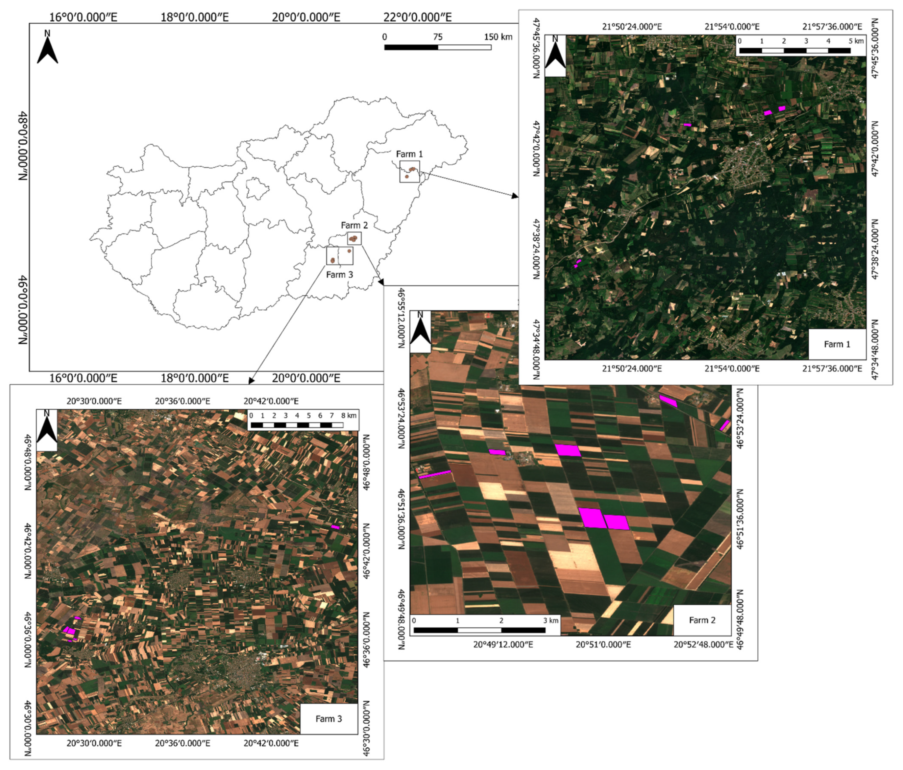
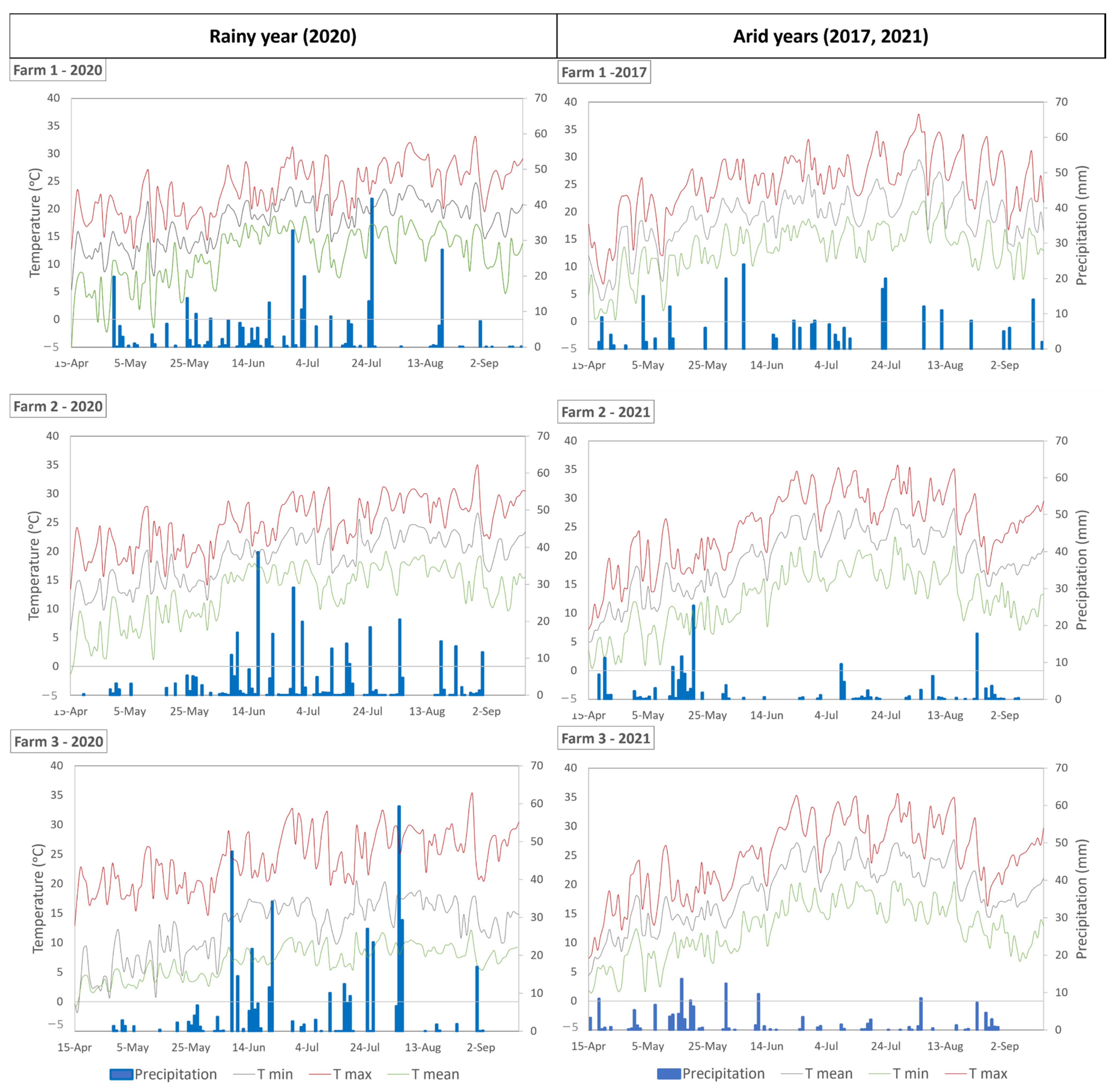
2.1. Study Area

Field investigations were conducted in north-eastern and south-eastern Hungary, with three farms participating (Figure 1). In 2017, field data were collected from 3 maize fields of Farm 1 (north-eastern Hungary). In this year, no other farm was included. In 2020, altogether, eleven fields were monitored. Three fields belonged to Farm 1, four fields belonged to Farm 2 (south-eastern Hungary), and the rest four belonged to Farm 3 (south-eastern Hungary). In 2021, three fields from Farm 2 and four from Farm 3 were involved. Two of the investigated fields were sweet maize in 2020 and 2021, and the rest were grain maize. Due to crop rotation, the observed fields were mostly different from year to year. The field coordinates are in

Table A1. Characteristics of each study field, sampling of cotton bollworm, and available satellite images for both satellites.

Year	Farm	Field	X	Y	Cultivation Purpose	Hybrid	Maturity Group 1	Adult Monitoring	Available Satellite Images
									Landsat-8	Sentinel-2
2017	Farm 1	F1_1	21.872793	47.714271	Grain maize	Amandha	FAO_400	Pheromone trap	4	11
2017	Farm 1	F1_2	21.921102	47.721464	Grain maize	Kinemas	FAO_300	Pheromone trap	4	11
2017	Farm 1	F1_3	21.807788	47.63241	Grain maize	KWS 2482	FAO_400	Pheromone trap	4	11
2020	Farm 1	F1_1	21.872793	47.714271	Grain maize	Kathedralis	FAO_400	Pheromone trap	3	7
2020	Farm 1	F1_4	21.928877	47.725272	Grain maize	Kathedralis	FAO_400	Pheromone trap	3	7
2020	Farm 1	F1_5	21.806356	47.629874	Grain maize	Durango	FAO_400	Pheromone trap	3	7
2020	Farm 2	F2_2	20.799724	46.872995	Grain maize	Fonard	FAO_400	None	6	10
2020	Farm 2	F2_3	20.886168	46.887758	Grain maize	P9486	FAO_300	None	6	10
2020	Farm 2	F2_4	20.86895	46.895381	Grain maize	DKC4943	FAO_300	None	6	10
2020	Farm 2	F2_5	20.817095	46.87975	Grain maize	Fonard	FAO_400	None	6	10
2020	Farm 3	Nm1	20.474071	46.608599	Sweet maize	SF1379	na	None	4	10
2020	Farm 3	Nm2	20.467449	46.610698	Sweet maize	Kiara	na	None	4	10
2020	Farm 3	F3_3	20.478401	46.600584	Grain maize	PR37N01	FAO_300	None	4	10
2020	Farm 3	F3_3	20.4809	46.62392	Grain maize	PR37N01	FAO_300	None	4	10
2021	Farm 2	Gy1	20.84142	46.881759	Grain maize	DKC4897	FAO_400	None	8	10
2021	Farm 2	Gy2	20.85435	46.859473	Grain maize	DKC4897	FAO_400	None	8	10
2021	Farm 2	Gy3	20.849997	46.858392	Grain maize	DKC4897	FAO_400	None	8	10
2021	Farm 3	Kd	20.772472	46.727483	Grain maize	PR37N01	FAO_300	Pheromone trap	8	10
2021	Farm 3	Nm1	20.474071	46.608599	Sweet maize	Kiara	na	None	8	10
2021	Farm 3	Nm2	20.467449	46.610698	Sweet maize	Kiara	na	None	8	10
2021	Farm 3	Nm5	20.471139	46.598485	Grain maize	PR37N01	FAO_300	Sex pheromone trap	8	10

¹ FAO type: FAO 300 maize type means, grain maize hybrids from FAO 290 to FAO 389, and FAO 400 type means, grain maize hybrids from FAO 390 to FAO 489.

in the Appendix A.

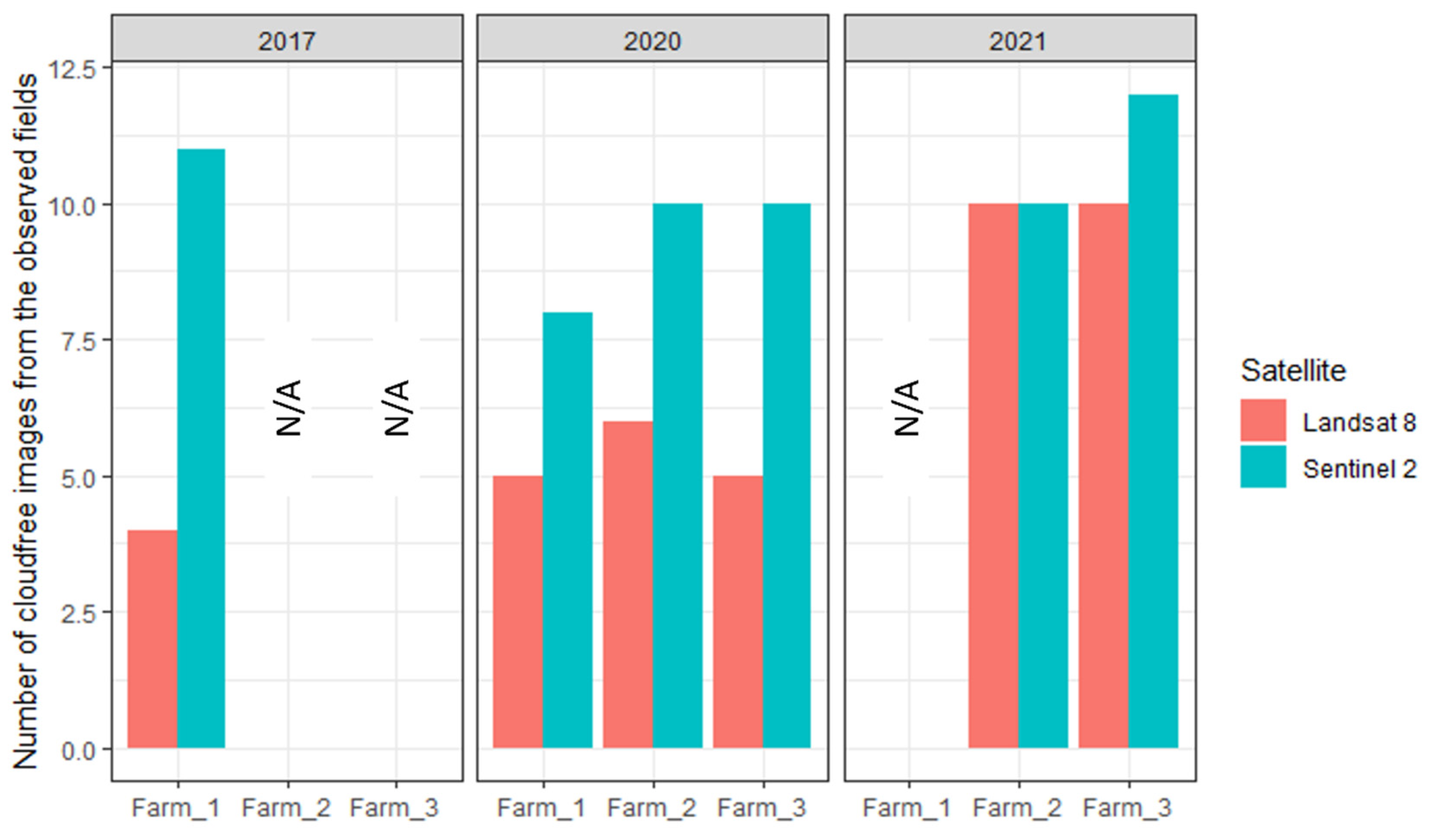
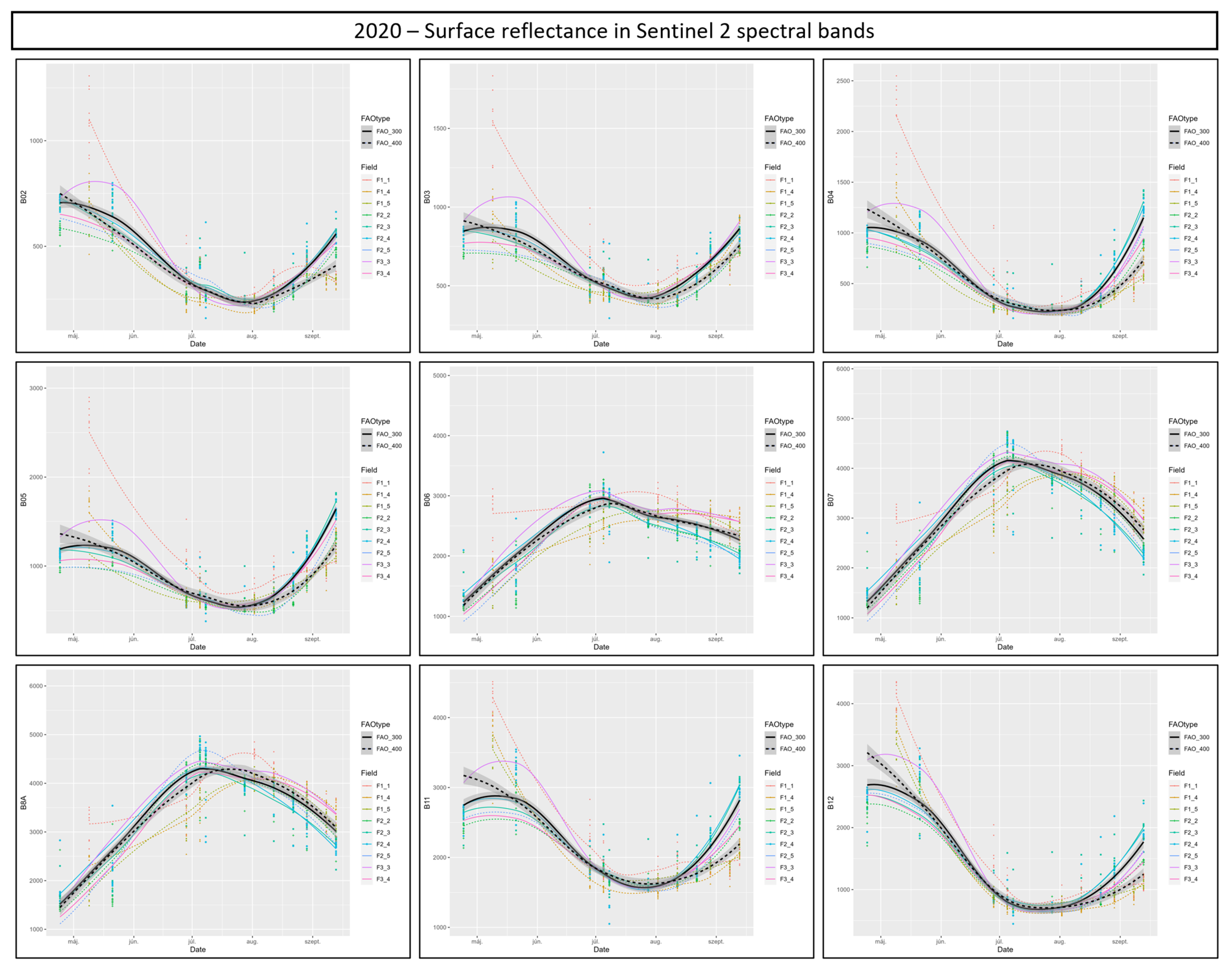
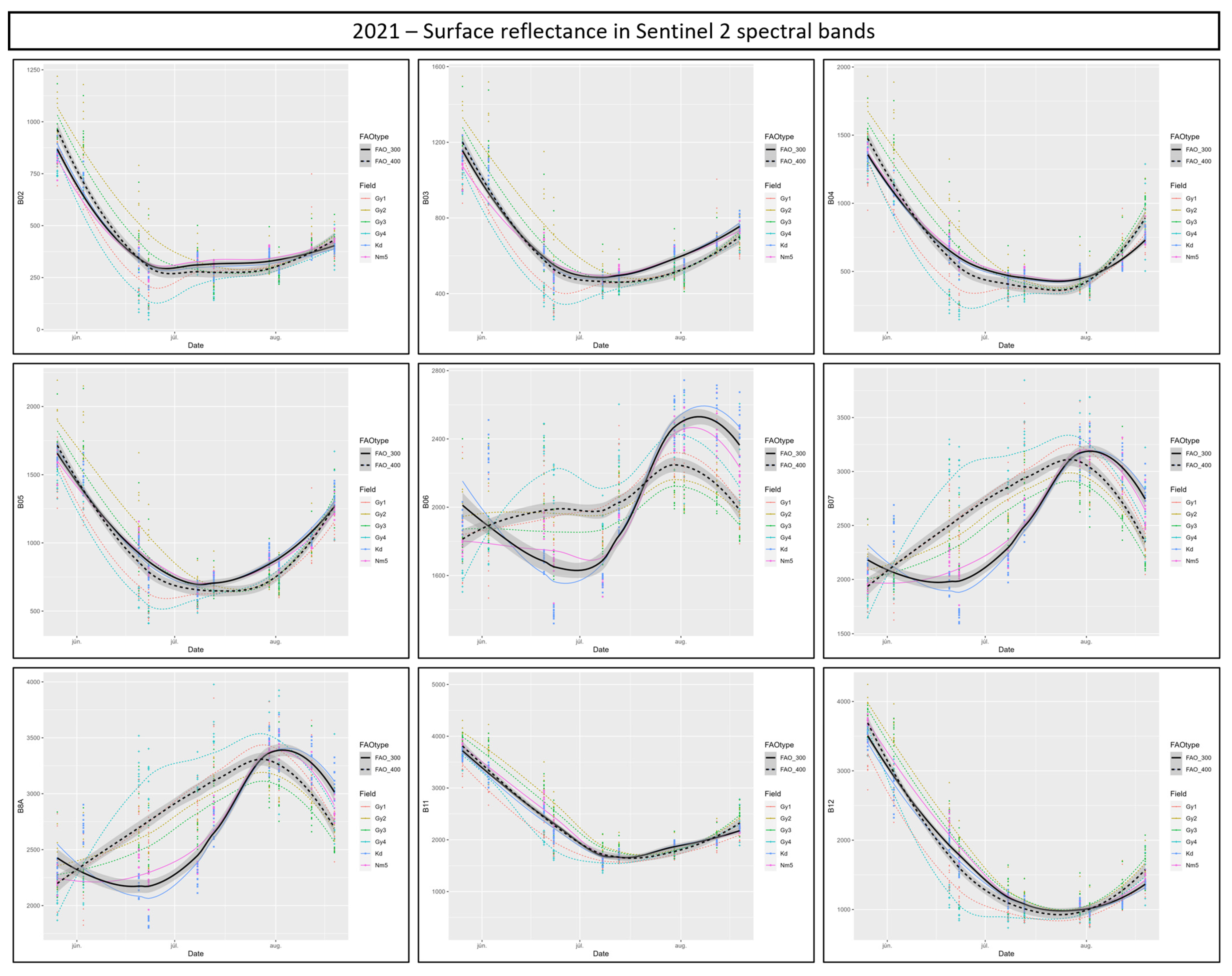
2.2. Satellite Remote Sensing Imagery Retrieving

Sentinel-2 images were provided by the ESA Copernicus Open Access Hub [76] at level 2A. Landsat images were obtained from Arlula [77] at level L1TP.

Landsat 8 and Sentinel-2 satellite images were collected with cloud cover below 60% (as only a tiny part of the picture was used). The recording time of the collected images was in the maize growing season (04.15–09.30 in 2017, 2020, and 2021).

All satellite images were collected with radiometric and geometric corrections previously applied by the providers. Sentinel-2 images at level 2A include a Scene Classification and an Atmospheric Correction providing Surface Reflectance data [78] that have been systematically generated using Sen2Cor processor [79]. Level-2A products included cloud and snow masks at a 60 m resolution. For the Landsat L1TP product, DOS1 atmospheric correction was applied in QuantumGIS (version 3.28.10) with a Semiautomatic Classification Pugin (SCP) developed by Condego [80]. An image was used only if all observed fields were cloud-free.

An extra quality control procedure was applied for sweet maize fields: the true color satellite images were visually reviewed in QGIS. The satellite image was excluded if the irrigation system (linear) was visible during the irrigation cycle (other than the zero position) and affected the selected sampling zones. This step could be omitted in grain maize fields, as none of the fields were irrigated.

Altogether, 101 satellite images (including Landsat 8 and Sentinel-2 products of all years and locations) were available. The spectral bands of the two satellites utilized in the study are listed in

Table 1. Considered spectral bands (‘B’) with their central wavelength and bandwidth and their original and processed resolution of Sentinel-2 and Landsat 8.

	Sentinel-2					Landsat 8
	Spectral Band	Central Wavelength (nm)	Bandwidth (nm)	Resolution	Resolution of Use (m)	Spectral Band	Central Wavelength (nm)	Bandwidth (nm)	Resolution	Resolution of Use (m)
Blue	B02	492.7	65	10	20	B2	482	60	30	30
Green	B03	559.8	35	10		B3	561.5	57	30
Red	B04	664.6	30	10		B4	654.5	37	30
Red-edge	B05	704.1	14	20
Red-edge	B06	740.5	14	20
Red-edge	B07	782.8	19	20
Near Infrared (NIR)	B08	832.8	105	10		B5	865	28	30
Short-Wave Infrared (SWIR)	B11	1613.7	90	20		B6	1608.5	85	30
Short-Wave Infrared (SWIR)	B12	2202.4	174	20		B7	2200.5	187	30

. The number of available recordings for each field and for both satellites are in Table A1 in the Appendix A.

2.3. Vegetation Index Selection and Calculation

To analyze the suitability of different vegetation indices (VIs) for CBW surveillance, 9 VIs were selected (

Table 2. Abbreviation, name, and formula of vegetation indices that were calculated based on Sentinel-2 and Landsat 8 spectral bands.

Abbr.	Name	Sentinel-2	Landsat 8
		Moisture-related vegetation indices
NDWI	normalized difference water index	$\frac{B03-B08}{B03+B08}$	$\frac{B3-B5}{B3+B5}$	[90]
NDMI	normalized difference moisture index	$\frac{B08-B11}{B08+B11}$	$\frac{B5-B6}{B5+B6}$	[91]
		Pigment-related vegetation indices
NPCRI	normalized pigment chlorophyll ratio index	$\frac{B04-B02}{B04+B02}$	$\frac{B4-B2}{B4+B2}$	[86]
ARI	anthocyanin reflectance index	$\frac{1}{B03}-\frac{1}{B05}$	-	[86]
CRI	carotenoid reflectance index	$\frac{1}{B02}-\frac{1}{B03}$	$\frac{1}{B2}-\frac{1}{B3}$	[87]
		General vegetation indices
EVI	enhanced vegetation index	$2.5\ast \frac{B08-B04}{B08+6\ast B04-7.5\ast B02+1}$	$2.5\ast \frac{B5-B4}{B5+6\ast B4-7.5\ast B2+1}$	[84]
NDVI	normalized difference vegetation index	$\frac{B08-B04}{B08+B04}$	$\frac{B5-B4}{B5+B4}$	[81]
SAVI	soil adjusted vegetation index	$1.5\ast \frac{B08-B04}{B08+B04+0.5}$	$1.5\ast \frac{B5-B4}{B5+B4+0.5}$	[82]
		Senescence- and ripening-related vegetation index
PSRI	plant senescence reflectance index	$\frac{B04-B02}{B06}$	$\frac{B4-B2}{B5}$	[85]

). The selection was based on two criteria: the index can be determined using Landsat 8 and/or Sentinel-2 spectral bands and has the potential to monitor or predict CBW damage. Three general VIs, namely the Normalized Difference Vegetation Index (NDVI), Soil Adjusted Vegetation Index (SAVI), and Enhanced Vegetation Index (EVI), were selected. We assumed that the number of CBW larvae and their damage depends on the coincidence of silking and the peak of adult appearance [13]. To characterize maize phenology, general VIs can be used. The NDVI was one of the earliest VIs created [81], and it can also be used to monitor maize phenology [47,54]. The SAVI was derived from the NDVI to reduce the noise generated by the reflectance of the soil [82]. Similar to the NDVI, the SAVI was able to estimate maize phenology [83]. By adding blue bands, the EVI was designed to be more sensitive to the structural variability of plant cover, surface type, and surface structure, and less sensitive to atmospheric effects and background noise [84]. As a signal of olfactory and color changes in maize, fruit ripening may affect the CWB oviposition preference. The Plant Senescence Reflectance Index (PSRI) has been proposed for determining the leaf aging and fruit ripening stage due to its sensitivity to plants’ carotenoid/chlorophyll ratio [85]. The discoloration can be important in host selection due to the CBW’s affinity for yellow [36] or blue [37]. Plants’ blue and purple discoloration is a result of anthocyanin pigments. The Anthocyanin Reflectance Index (ARI) is sensitive to the anthocyanin pigment concentration in the leaves [86], whereas the CRI (Carotenoid reflectance vegetation index) is used to measure the overall carotenoid content of the leaves [87]. Plant water stress has been determined to affect the CBW’s preference for oviposition and feeding performance [88]. The NDMI has been commonly used to monitor forest ecosystem moisture, and thus, the overall forest health and condition [89], while the NDWI has been developed to indicate the water content and availability [90]. VIs were calculated from Landsat 8 and Sentinel-2 recordings (Table 2). The reflectance measurements retrieved from Landsat 8 and Sentinel-2 satellites differ in spectral resolution. The bands of the satellites cover different wavelengths in certain spectral ranges. The bands’ central wavelengths are also different (Table 1). Therefore, the value of a VI calculated from the bands of the two satellite sensors differ due to the wavelengths covered [40]. Different atmospheric correction models were used for pre-processing the images of the two satellites, which also influenced the value of the VI [60]. Therefore, the two satellites’ performance were compared to determine their efficacy for the surveillance of the CBW larval ear damage.

2.4. Cotton Bollworm Larval Damage Observations

The following intra-field sampling method was applied for the distribution analysis of maize ear damage caused by CBW larvae (Figure 2):

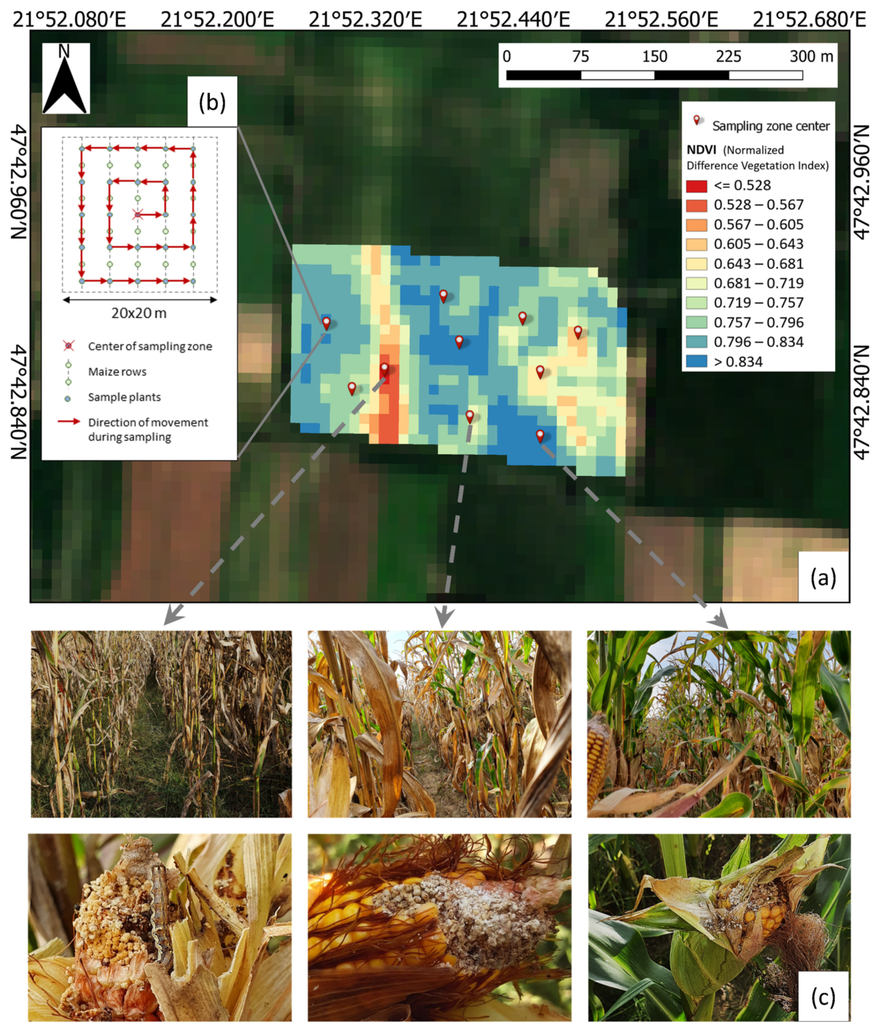
• Sampling zone selection: Georeferencing of field boundaries was performed manually. For each field, the NDVI was calculated based on Sentinel-2 imagery with a 20 m spatial resolution, and a grid of 20 × 20 m zones was applied to the fields. Ten sampling zones were selected in each field by the following method: The field’s NDVI values range was divided into ten equal sub-ranges. From each sub-range, one sampling zone was selected.
• Deploying sampling zones: The center point of the selected sampling zones was retrieved in QGIS and deployed on the fields based on GPS coordinates using a Trimble Juno 3B GPS device.
• Sample plant selection: In each sampling zone, 36 sample plants were selected following a spiral line from the sampling zone’s center with an equal distribution on the zone’s grid points.
• Damage observation: The ears of sample plants were visually inspected. The presence of apparent CBW larvae damage was observed by removing the ears’ husk and checking for chowed kernels and the typical excrement of the CBW (Figure 2). The extent of the damage to the ears was assumed to be negligible information and not estimated. The percentage of damaged ears was considered as characteristic of the sampling zone.

Field observations were conducted in the first week of August in sweet maize fields in 2020 and 2021. In grain maize fields, the larval damage distribution was investigated in the first week of September 2021 and in the second week of September 2017 and 2020. During 2017, 2020, and 2021, altogether, 7560 plants were visually inspected on the three different farms in the sampling zones of different maize fields.

As a quality control measure of the field data, some sampling zones were excluded from the data analysis due to the following reasons:

• maize plant density dropped below 60% due to waterlogging;
• maize plant density dropped below 60% due to agronomic failure;
• a large object was found in the sampling zone (e.g., light pole)

2.5. Cotton Bollworm Adult Flight Monitoring

Adult CBW flight activity was observed in particular fields (Table A1 of the Appendix A). For adult monitoring, CSALOMON^® VARL funnel sex pheromone traps (Plant Protection Institute CAR, ELKH, Budapest, Hungary, www.csalomoncsapdak.hu, (accessed on 28 May 2023) were used, where a CBW sex pheromone lure was used as an attractant [4]. The traps were fixed to a 200 cm tall wooden pole. The pheromone attractant was a pheromone-impregnated rubber ring attached to a plastic sheet fixed to the trap’s upper portion. For CBW termination, lambda-cyhalothrin insecticide was used on a 3-by-3 cm sponge. The trap was placed on the field 200 m from the boundary. In 2017, adult flight activity was observed in all fields. In 2020, adult flight activity was observed at Farm 1 and in 2021 at Farm 3, according to Table A1. Each year, traps were installed at the end of May and maintained until the beginning of September. The number of captured adults was counted weekly in all traps.

2.6. Additional Field Observations

Maize phenology was recorded, as it affects the host selection of CBW adults, larval feeding, and subsequent damage. Phenology was grouped according to the general BBCH scale [92]:

• BBCH 05–BBCH 17   Emergence, establishment, and mid-early development
• BBCH 18–BBCH 52   Canopy closure, organ, and stem elongation
• BBCH 53–BBCH 64   Tasseling, silking, pollination, and fertilization
• BBCH 65–BBCH 84   Grain filling
• BBCH 85–BBCH 89   Physiological maturation
• BBCH 99–       After harvest

The maize hybrids of the observed fields were recorded as a field characteristic (Figure A1 of the Appendix A). The different maize hybrids were classified based on their cultivation purposes (sweet maize–commercial grain maize fields). Commercial grain maize fields were subdivided according to the maturity group of the maize hybrids planted in the field (based on their FAO numbers [93]). Two maturation categories were used:

• FAO 300 maize hybrids: consists of mid–early maturing grain maize hybrids from FAO 290 to FAO 389;
• FAO 400 maize hybrids: consists of mid–late maturing grain maize hybrids from FAO 390 to FAO 489.

Meteorological data (minimum, maximum, average daily temperature, and daily sum of precipitation) were also recorded and plotted in Figure A1 annually by farm. The weather during the maize growing season was more arid in 2017 and 2021. The sum of precipitation was 255 mm in Farm 1 in the maize growing season of 2017. In 2021, the sum of precipitation was 180 mm in Farm 2 and 138 mm in Farm 3. In contrast, the weather in 2020 was more humid on all surveyed fields; the rainfall was 323 mm, 333 mm, and 394 mm in Farm 1, Farm 2, and Farm 3, respectively.

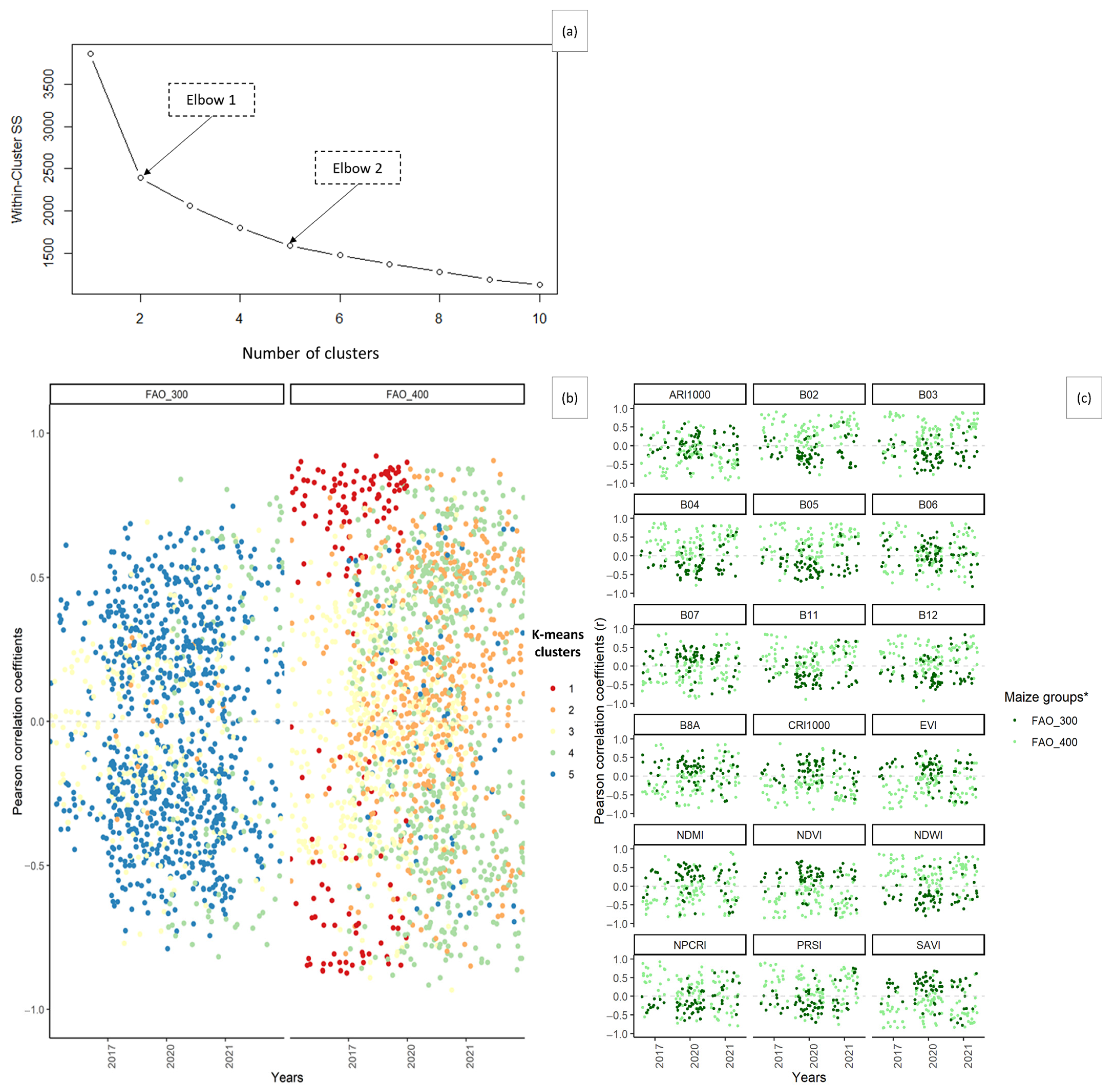
2.7. Statistical Analysis and Visualization

We would like to establish the existence of the relationship and its circumstances between the CBW larval damage (percentage of ears damaged) in the sampling zones and their surface reflectance on different bands of Landsat 8 and Sentinel-2 or VIs. Correlations were therefore estimated between the damage and the spectral data. The relationship was evaluated in terms of a correlation analysis over each field and each date.

As the data did not deviate significantly from a normal distribution, we used the Pearson correlation method, and Pearson correlation coefficients (PCCs) were calculated for each field and date separately. Correlations were deemed to be significant when p < 0.05. For the interpretation of correlation coefficients,

Table 3. Interpretation of correlation coefficients of Pearson correlation analysis.

Pearson Correlation Coefficient		Interpretation
−1	1	Perfect
−0.95–−0.99	+0.95–+0.99	Very Strong
−0.75–−0.95	+0.75–+0.95	Strong
−0.3–−0.75	+0.3–+0.75	Moderate
−0.1–−0.3	+0.1–+0.3	Low
0–−0.1	0–+0.1	No correlation

was considered [94].

In order to clarify the paired data, where the PCCs were calculated, we present the data structure below (Figure 3).

In order to explore the agricultural meanings of the correlations, we grouped the PCCs by satellite, and by bands and VIs. The PCCs of the groups were inconsistent (see Section 3.3). As a consequent step, in order to find patterns of the PCCs, a K-means clustering analysis [95] was conducted on the PCCs of each spectral band and VI, considering other field parameters such as farm, date, maize cultivation purpose, and maturity group. The Within-Cluster Sum of Square elbow method [95] was used to find the optimal number of clusters.

From the results of the K-means clustering analysis, we could identify the relevant factors for the consistency of the PCCs. After identifying the relevant agronomic groups, we could search for the highest PCCs with respect to time along with phenology, spectral bands, and VIs.

The differences among groups of Pearson correlation coefficients (PCCs) were analyzed by ANOVA and post hoc tests (Tukey’s Honest Significant Difference (Tukey HSD)) since ANOVA and Tukey HSD tests are standard methods to compare more than two means. The difference was considered as significant when p < 0.05. ANOVA and Tukey HSD tests were conducted only when the PCCs satisfied all criteria of ANOVA and Tukey HSD tests (e.g., grouped data were independent). We found that Mengarelli’s method (of performing ANOVA tests on Spearman correlation coefficients) was suitable whenever differences between the PCC groups were examined [96].

When assumptions of the ANOVA test were not fulfilled, only the mean, median, and standard deviations were analyzed. In the correlation strength analysis, the absolute values of the PCCs were used, which is similar to the approach used in remote sensing research, where the suitability of the VIs for different purposes are compared [97].

ANOVA and Tukey HSD tests were also applied for the damage percentages of the sampling zones. Differences were determined among fields, farms by each year, and years. The significance of variance analysis and pairwise comparisons were analyzed considering an error probability < 0.05.

To estimate the dependence of the correlations (grouped PCCs) on time, linear regression models were also fit on the grouped PCCs (this approach has been recently used in healthcare research [98]) to find whether the changes in the PCCs have a time dependency (week of the year). The significance of the linear models was analyzed considering an error probability < 0.05.

The analysis and visualization were made by Microsoft Excel (version 2310), Visplore (version v2023a) [99], and R Studio (version 2022.07.02) [100] with the use of the packages ‘reshape’ [101], ‘ggplot2’ [102], ‘dplyr’ [103], ‘emmeans’ [104], and ‘multcomp’ [105].

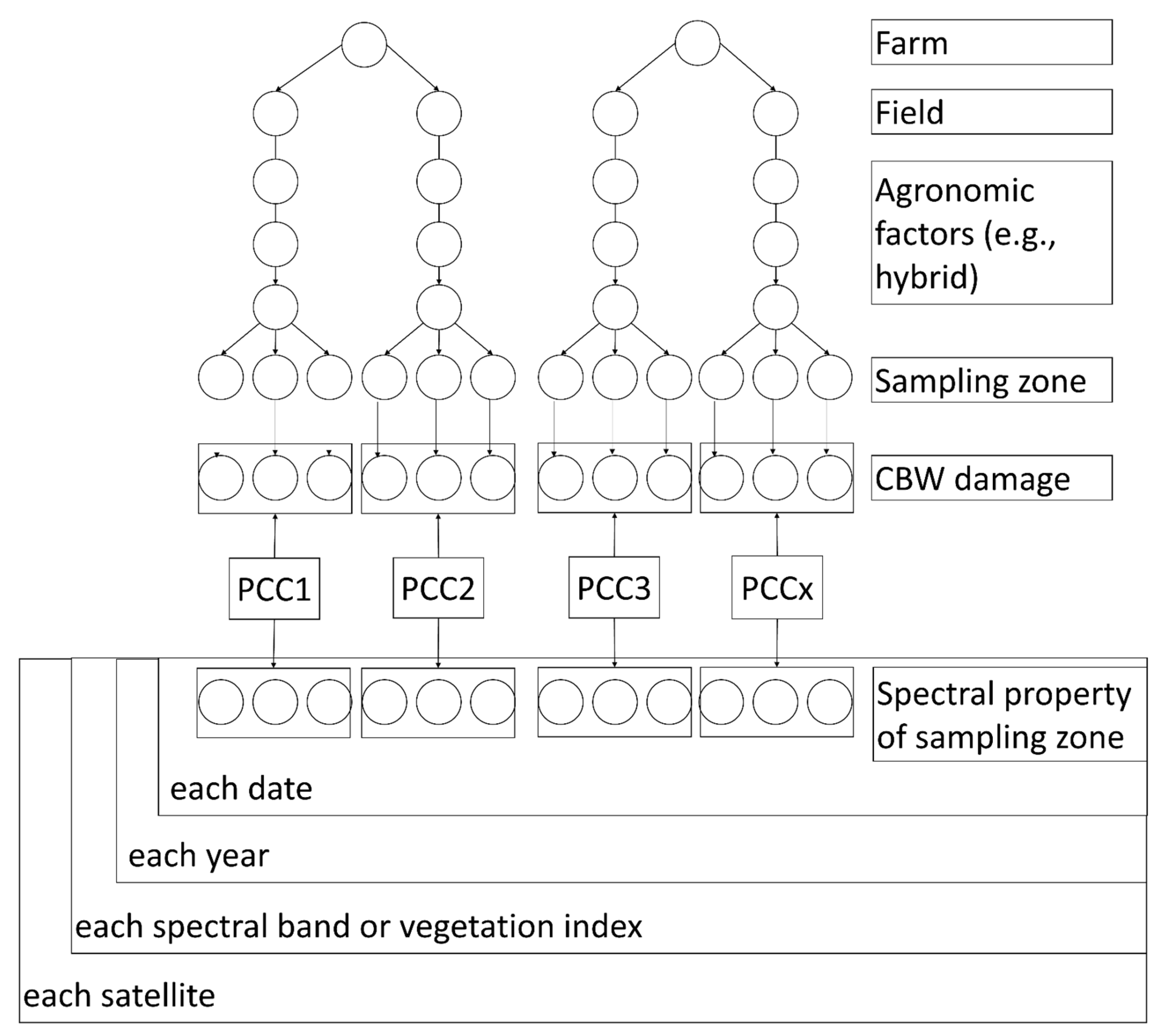
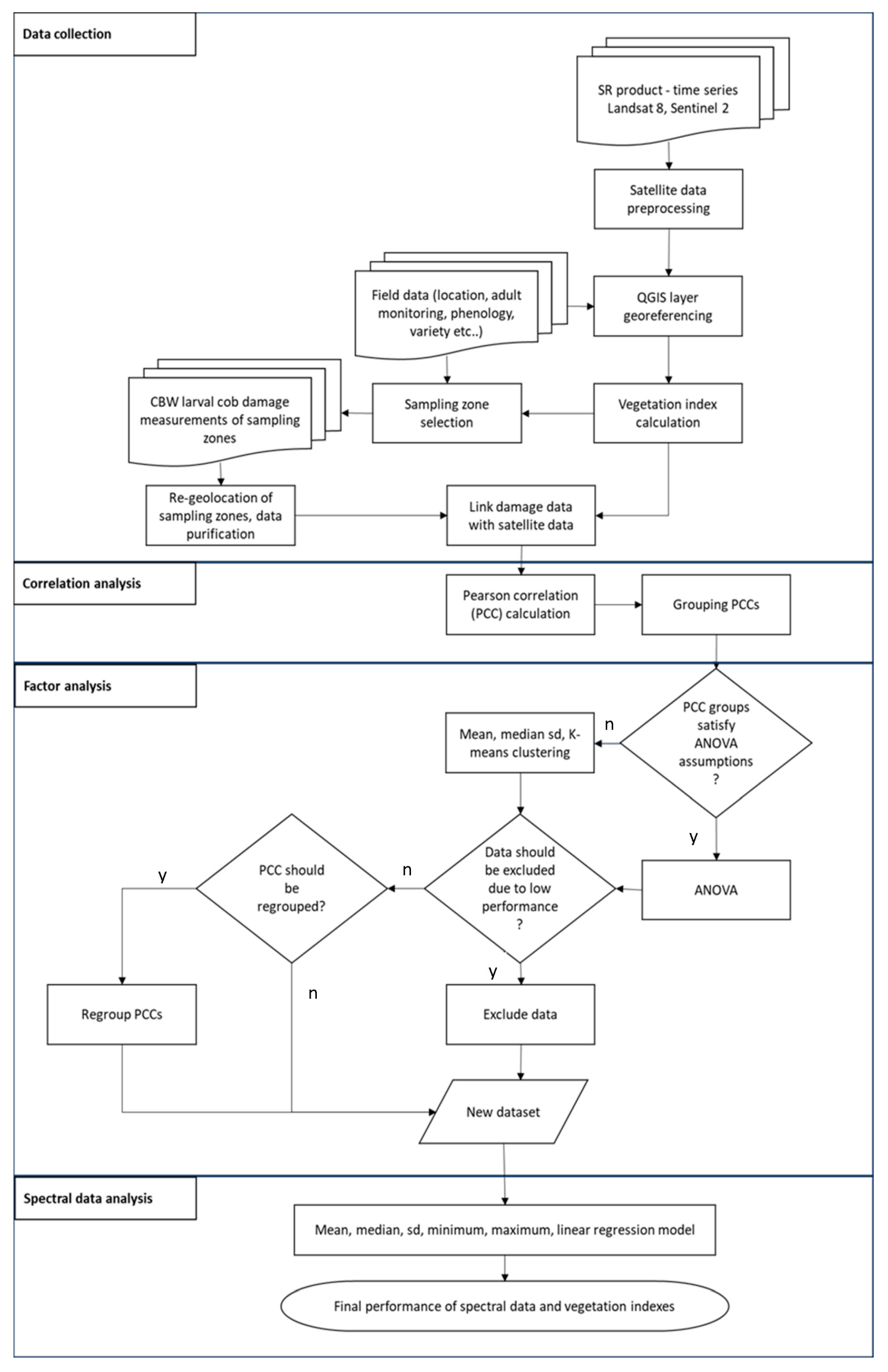
2.8. Summary of Methodology

Field observations were conducted in north-eastern and south-eastern Hungary, with 21 fields on three farms. On-farm investigations were conducted in 2017, 2020 and 2021. Satellite images of Landsat-8 and Sentinel-2 were collected. VIs were selected based on two criteria: they can be determined using Landsat-8 and/or Sentinel-2 bands and have the probability to be impacted by CBW feeding. The selected VIs are as follows: EVI, NDVI, SAVI, NDMI, NDWI, ARI, CRI, NPCRI, and PSRI. Intra-field, NDVI-based sampling methods were used to measure damage distribution. Adult CBW flight activity was observed with CSALOMON^® VAR-type traps. Pearson correlation coefficients between the ear damage caused by CBW larvae and the surface reflectance (recorded by Landsat 8 and Sentinel-2) or VIs (computed using surface reflectance) were calculated field-by-field (PCCs). The strength of correlations was analyzed by converting the PCCs to absolute values.

The correlation results were analyzed by examining differences between multispectral satellites, spectral ranges and VIs, date (calendar week, thus coincidence of important crop phenology and CBW flight activity), farm, and field. It must be highlighted that these factors may also affect each other. The reflectance was measured on different dates, and the maize hybrids were also different annually in the investigated fields (due to crop rotation). ANOVA and Tukey HSD post hoc tests and K-means clustering and linear regression models were used to evaluate the correlation between the percentage of ears damaged and the VIs. Data were processed according to Figure 4. The aim of this analysis was to determine which parameters, under which conditions, should be considered or removed from the model, leading to the highest PCCs trend-wise.

3. Results

3.1. Cotton Bollworm Larval Damage to Maize Ears on Fields, Farms, and Years

Although the weather conditions in the sampling years were different, the yearly average ear damage on all farms and fields was similar, around 35% each year. Damage appeared highly variable (

Table 4. Larval damage of cotton bollworm to maize fields in each farm and year.

Year	Farm	Field	Cultivation Purpose	Mean ± SD 1			CLD 2	Median	Min	Max	CV 3	Mean ± SD of Farms			CLD	Mean ± SD of the Year			CLD
2017	Farm 1	F1_1	Grain	48.8	±	11.9	abc	47.0	28.0	68.8	0.24	35.6	±	14.7	AB	35.6	±	14.7	a
		F1_2	Grain	32.1	±	6.7	adefg	33.3	19.4	38.9	0.21
		F1_3	Grain	23.0	±	10.8	ehi	20.8	8.3	39.4	0.47
2020	Farm 1	F1_1	Grain	53.9	±	18.6	bc	53.5	19.4	80.6	0.35	46.9	±	14.3	A	34.5	±	16.7	a
		F1_4	Grain	44.7	±	10.8	bf	46.0	29.7	67.7	0.24
		F1_5	Grain	40.0	±	6.5	efg	41.7	33.3	50.0	0.16
	Farm 2	F2_2	Grain	43.2	±	7.9	cf	44.6	29.7	59.5	0.18	34.5	±	10.4	BC
		F2_3	Grain	34.1	±	9.5	adefg	31.1	24.3	51.3	0.28
		F2_4	Grain	30.4	±	10.8	defg	25.7	16.2	48.7	0.35
		F2_5	Grain	31.1	±	9.0	defg	29.7	18.9	48.7	0.29
	Farm 3	Nm1	Sweet	21.0	±	12.9	dhi	14.3	8.6	42.9	0.61	25.8	±	18.5	B
		Nm2	Sweet	1.7	±	2.4	j	0.0	0.0	5.7	1.40
		F3_3	Grain	41.7	±	5.4	cfg	41.4	31.4	51.4	0.13
		F3_4	Grain	38.3	±	11.5	cefg	37.1	20.0	60.0	0.30
2021	Farm 2	Gy1	Grain	26.2	±	12.1	gi	23.0	10.8	48.7	0.46	30.5	±	12.6	BC	32.4	±	20.0	a
		Gy2	Grain	38.6	±	11.1	cefg	33.8	24.3	54.0	0.29
		Gy3	Grain	26.5	±	11.4	gi	24.3	16.2	54.0	0.43
	Farm 3	Kd	Grain	60.0	±	8.7	b	58.0	44.0	76.0	0.14	37.2	±	25.6	AC
		Nm1	Sweet	10.5	±	4.8	ij	10.0	4.0	20.0	0.45
		Nm2	Sweet	6.3	±	3.9	hj	4.0	4.0	12.0	0.62
		Nm5	Grain	54.7	±	7.2	bc	52.0	44.0	68.0	0.13
All				33.9	±	17.7		33.3	0.0	80.6	0.5

¹ SD = standard deviation of mean. ² CLD = Compact letter display of groups (ANOVA, Tukey’s post hoc). ³ CV = Coefficient of variation.

). The percentage of damaged ears on the farms were different in different years. The average damage on Farm 3 was significantly higher (p < 0.01) in 2021 (37.2 ± 25.6) than in 2020 (25.8 ± 18.5). The average damage on Farm 1 was higher in 2020 than in 2017 (46.9 ± 14.3 and 35.6 ± 14.7, respectively). Still, the difference was insignificant (p = 0.14) due to the high within-field variability of the damage (SD ranging from 6.5 to 18.6). There were significant differences between the average damage on the farms in the same year. In 2020, the damage was significantly higher on Farm 1 (46.9 ± 14.3) than on Farm 2 (34.5 ± 10.4, p = 0.01).

There were significant differences among the damages to the fields, even if they were measured in the same year and farm. On Farm 1, there was a significant difference among the fields in both years (F1_1 versus F1_3 (p < 0.01) in 2017 and F1_1 versus F1_5 (p = 0.03) in 2020 Table 4). On Farm 2, there was no significant difference among the fields. On Farm 3, there were significant differences between damage to commercial grain maize fields and sweet maize fields in 2020 and 2021 (Table 4).

The intra-field variability of the damage was high in each year and at each farm in each field (Table 4). The SD of the fields ranged from 2.4 (Nm2) to 18.6 (F1_1), and the coefficient of variation ranged from 0.13 (Nm5) to 0.62 (Nm2).

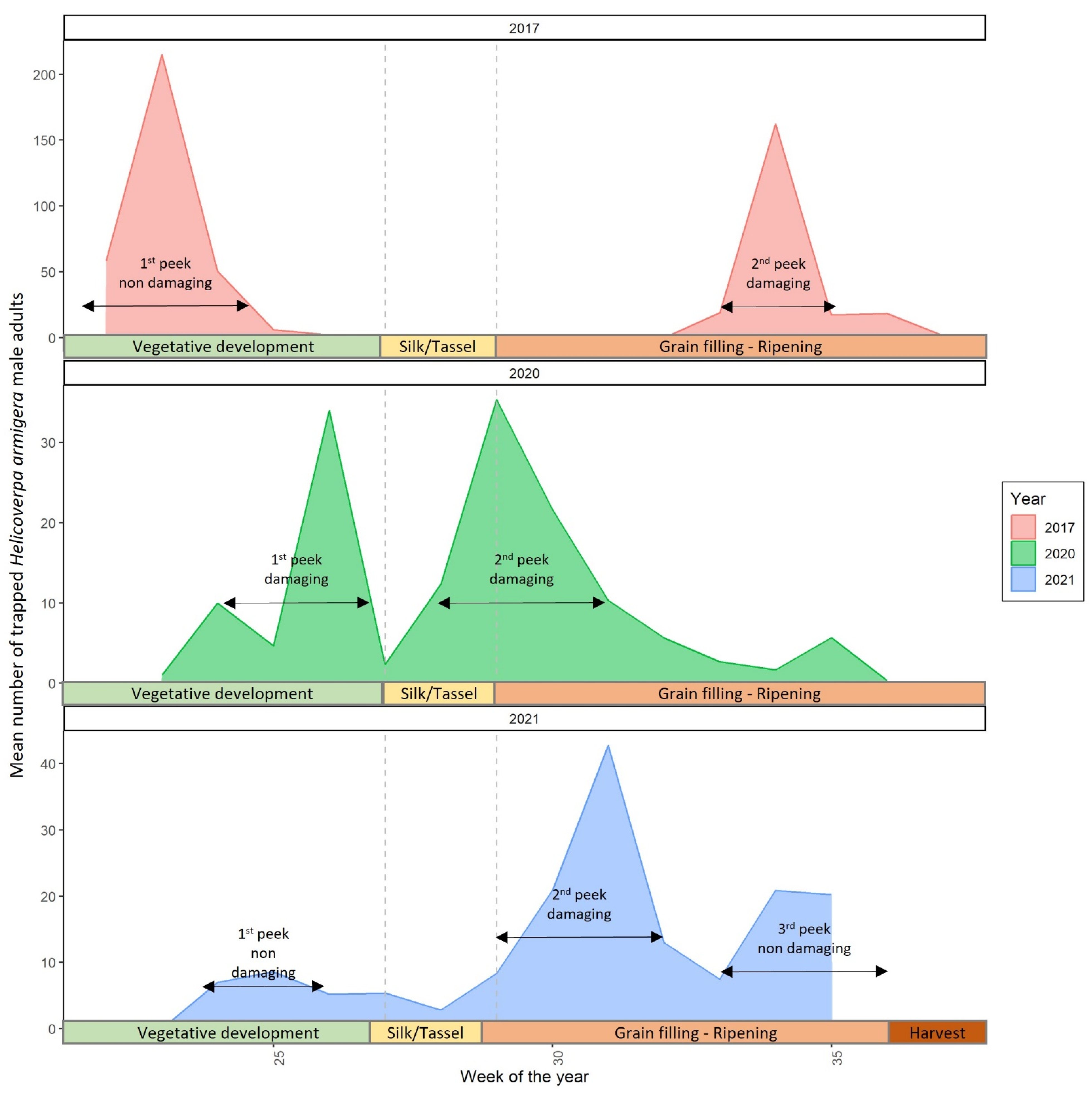
3.2. Cotton Bollworm Adult Monitoring and Annual Peaks of Their Appearance

The prediction and monitoring of CBW damage rely on the concurrence of generative maize phenological stages (silking and tasseling) and the peak density of adult populations. If the peak occurs during the vegetative developmental stage of maize plants, long before silking, the maize plant will not be damaged. If the silking and CBW adult population density peak are close to each other, or the peak occurs during the reproductive phenological stage, the maize ears will be damaged.

In our study, the period of CBW adult flights varied between years (Figure 5). In 2017, two adult population peaks were observed, and only the second peak resulted in ear damage. In 2020, both generations resulted in damaged maize ears as both peaks were close to silking. In 2021, three peaks were observed. The first peak appeared during the vegetative development of the maize, unlikely affecting maize ears. The second peak appeared two weeks after silking and highly influenced the ear damage. The third generation appeared late when the maize grains were close to physiological maturity and, therefore, had little impact on damage.

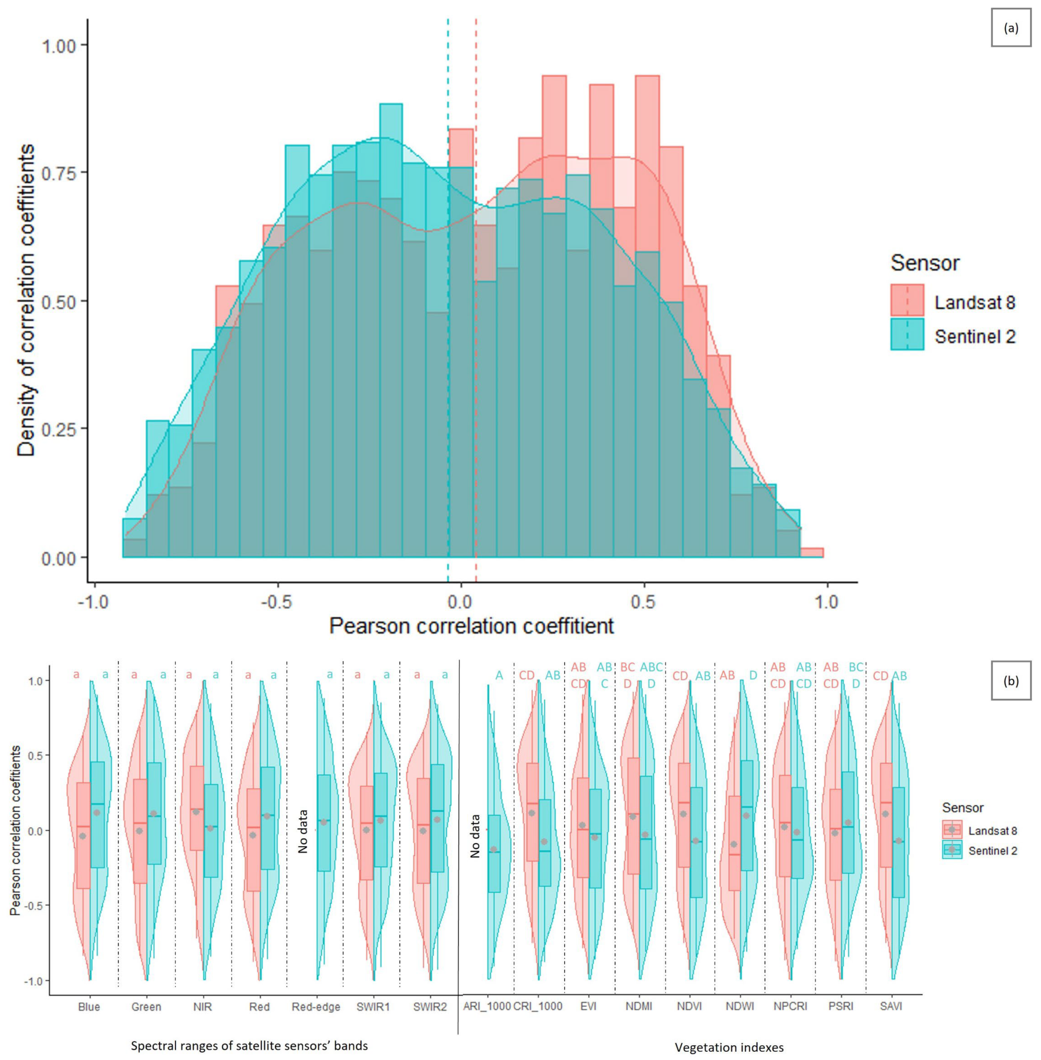
3.3. Suitability of Landsat 8 versus Sentinel-2 Satellites for Cotton Bollworm Damage Surveillance in Maize

Pearson correlation coefficients (PCCs) of the ear damage caused by CBW larvae, with surface reflectance (recorded by Landsat 8 and Sentinel-2) or VIs (computed using surface reflectance), showed a wide range from no correlation to a correlation up to r = +/−0.93, regardless of the satellite. Although the PCCs showed different distribution patterns when the bands and VIs of the two satellites were compared, the correlation strengths were not considerably different. Sentinel-2 bands and indices reached higher correlation strengths, regardless of the chosen band or VI (Figure 6 and

Table 5. Pearson correlation coefficients between ear damage caused by cotton bollworm larvae and spectral bands or vegetation indices of Sentinel-2 and corresponding Landsat 8 satellite imagery.

Sentinel-2					Landsat 8
	Mean	SD	Min	Max		Mean	SD	Min	Max
B02	0.11	0.42	−0.85	0.90	B2	−0.04	0.40	−0.84	0.65
B03	0.11	0.44	−0.86	0.90	B3	0.00	0.42	−0.84	0.69
B04	0.09	0.42	−0.86	0.87	B4	−0.03	0.40	−0.88	0.72
B05	0.10	0.43	−0.89	0.88
B06	0.04	0.42	−0.89	0.88
B07	0.01	0.42	−0.86	0.86
B8A	0.01	0.42	−0.84	0.85	B5	0.12	0.38	−0.72	0.80
B11	0.06	0.39	−0.92	0.85	B6	0.00	0.38	−0.87	0.65
B12	0.07	0.42	−0.93	0.84	B7	−0.01	0.40	−0.92	0.67
ARI*1000	−0.13	0.38	−0.92	0.79	CRI*1000
CRI*1000	−0.08	0.40	−0.89	0.87		0.11	0.41	−0.76	0.93
EVI	−0.05	0.41	−0.87	0.86	EVI	0.03	0.42	−0.80	0.90
NDMI	−0.04	0.45	−0.82	0.90	NDMI	0.09	0.43	−0.70	0.92
NDVI	−0.08	0.43	−0.85	0.84	NDVI	0.10	0.41	−0.76	0.79
NDWI	0.09	0.43	−0.82	0.88	NDWI	−0.10	0.39	−0.73	0.75
NPCRI	−0.02	0.40	−0.80	0.92	NPCRI	0.02	0.42	−0.88	0.85
PSRI	0.04	0.41	−0.85	0.89	PRSI	−0.02	0.41	−0.88	0.80
SAVI	−0.08	0.43	−0.85	0.84	SAVI	0.10	0.41	−0.76	0.79
All	0.015	0.42	−0.93	0.92	All	0.021	0.41	−0.92	0.93

), which is likely due to the more frequent cloud-free images. Therefore, Sentinel-2 was slightly better for CBW surveillance than Landsat 8.

The average value of all Pearson correlation coefficients (PCCs) was 0.017 ± 0.42 and 0.37 ± 0.22 when the absolute value of the PCCs was considered. Moderate correlations were found to be more frequent. All measured bands and vegetation indices (VIs) of the two satellites were collectively analyzed (Figure 6a), as well as the bands and indices separately (Figure 6b). When analyzing all correlations collectively by satellite (considering all bands, all VIs, dates, farms, and fields), the PCCs had no significant difference between the two satellites (Figure 6a). The density of the PCCs exhibits dual peaks around −0.3 and +0.3 for both satellites, denoting that moderate correlations are the most frequent for both satellites. The peak at −0.3 is slightly higher for Sentinel-2. In contrast, Landsat 8 has a higher peak at +0.3 to +0.5, implying that some of the parameters of the satellites may influence the suitability of their imagery for CBW surveillance.

The differences of the PCCs of VIs and the bands of the two satellites are presented in Figure 6b and Table 5. The mean, median, minimum, and maximum values of the PCC groups were analyzed. There was no significant difference between the mean of the PCCs based on the different satellite bands, neither between the satellites nor the different spectral ranges (Figure 6b). There was no significant difference when only the mean of the absolute values of the PCCs were considered. However, the Sentinel-2 satellite had stronger maximum positive PCCs and stronger negative minimum PCCs in almost all bands in a trend-wise manner (92% of all extremes of Sentinel-2 PCCs was higher Table 5).

The mean PCCs of the two satellites’ VIs differed from each other (Figure 6b and Table 5). Moreover, there were significant differences between the same VI’s PCCs derived from the two different satellites. The NDWI and PSRI, derived from Sentinel-2, had higher PCCs than the other indices. As for Landsat 8, only the NDWI’s PCCs were significantly stronger (lower in the negative range) than the other VIs. Comparing the same VIs of the two satellites, CRI, NDWI, NDVI, and SAVI produced significantly different PCC means and distributions (Figure 6b). The CRI, NDVI, and SAVI based on Sentinel-2 showed rather negative PCCs, while the same indices based on Landsat 8 showed rather positive PCCs. In the case of the NDWI, only the strength of the correlation was similar, but the direction was not. In general, the Sentinel-2 satellite produced stronger maximum positive PCCs and stronger negative minimum PCCs, and 69% of all extremes of PCCs (regarding the satellites’ bands, Table 5).

Although there were differences in the distributions of the PCCs of the spectral bands and VIs derived from the two satellites, the mean of the absolute value of the correlations was not significantly different. However, the maximum correlation strengths were higher with Sentinel-2 reflectance measurements (regarding the majority of the bands and VIs); altogether, 82% of all extremes of the PCCs (regarding the vegetation indexes) were stronger, which was likely due to the shorter orbiting period with a higher number of retrievable cloud-free images (Figure 7). Moreover, cloud-free images are more likely to be captured during the growing season. The number of cloud-free images ranged from three to eight considering Landsat, while the number ranged from seven to eleven considering Sentinel-2. Landsat 8 provides 20–64% fewer cloud-free images than Sentinel-2. Therefore, only Sentinel-2 satellite-derived images are considered in the following sections.

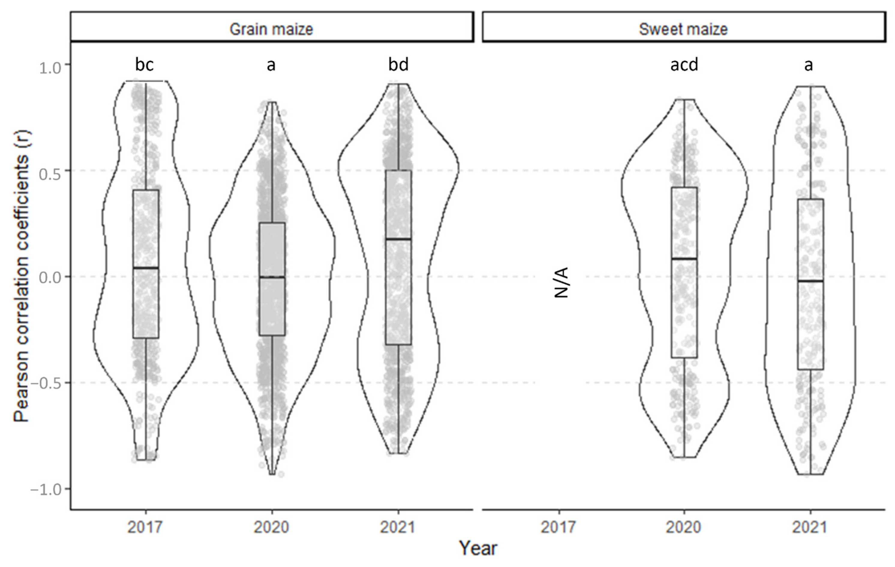
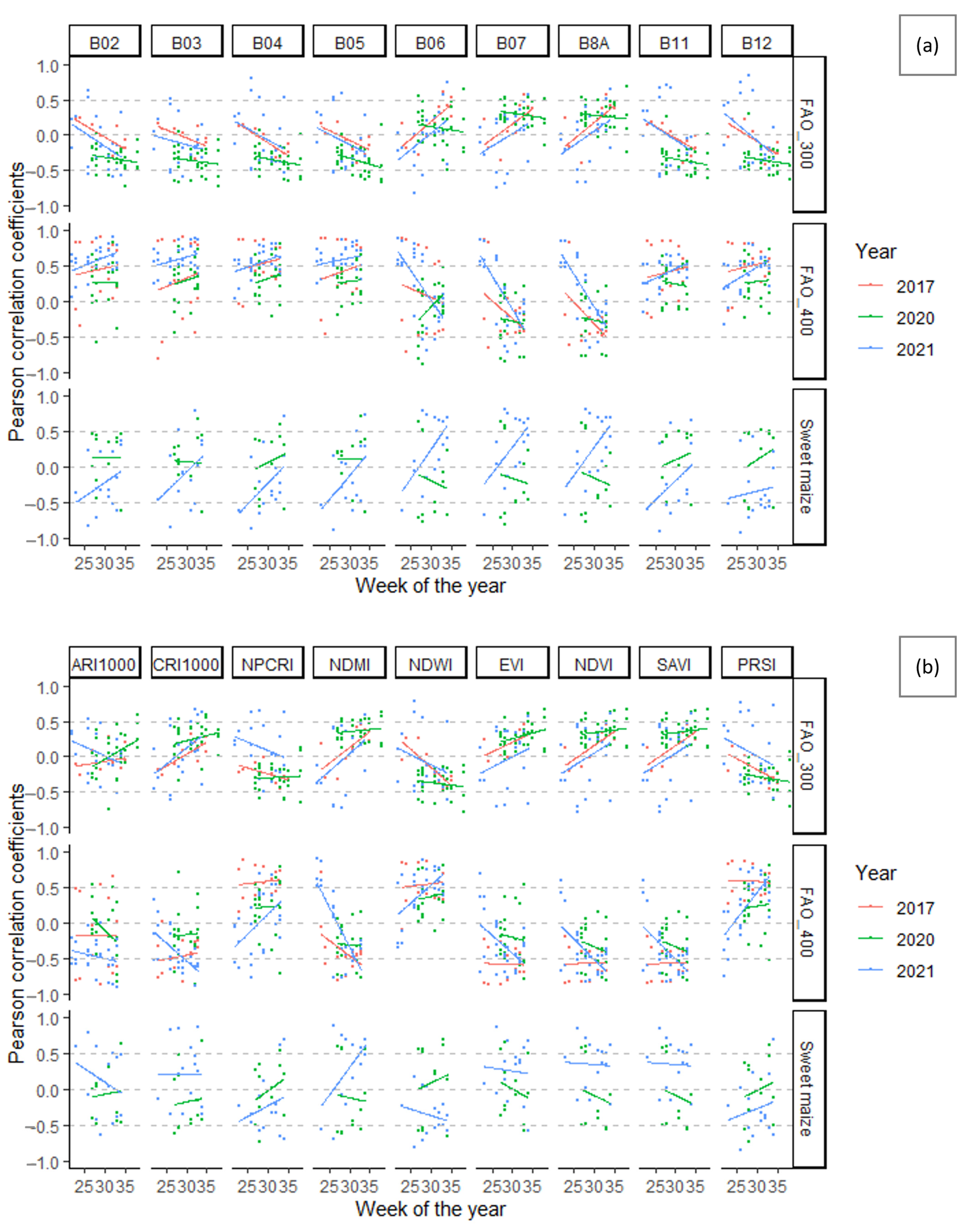
3.4. Cotton Bollworm Surveillance via Remote Sensing, Depending on Year, Maize Cultivation Purpose, and Maturity Group

In the following sections, correlations between CBW damage with the Sentinel-2 recorded surface reflectance and VIs were investigated, and similar and distinct repetitive patterns were found among the correlations over all recorded spectral and field data. One of the major contributors to the observed PCCs was the year, as the weather conditions of these years differed (Table A1). Another important factor of the PCCs was the maize cultivation purpose (sweet or grain maize) and maturity group of the grain maize hybrids. The PCCs showed a similar pattern in the two arid years (2017 and 2021) and differed in the humid year (2020). There were also significant differences between sweet and grain maize fields’ PCCs (Figure 8).

The PCCs and correlation strengths were compared year-by-year and between sweet and grain maize. In each year, the mean values of the PCCs (considering grain maize in 2017, 2020, and 2021, as well as sweet maize in 2020 and 2021) were around zero (0.07, −0.02, 0.09, 0.03, and −0.03, respectively). The PCCs had a negative and a positive density peak in fields with both cultivation purposes. For the sake of accuracy, the strength of the PCCs were used. The mean of correlation strength was around 0.40 (grain maize 2017 = 0.39, grain maize 2021 = 0.38, sweet maize 2020 = 0.41, and 2021 = 0.42), except for grain maize fields in 2020, where the mean (0.29) was significantly (p < 0.01) lower than in the other years. There were no significant differences between the PCCs in grain maize in 2017 and 2021. However, in 2021, the PCCs of sweet maize fields were significantly stronger than the PCCs of grain maize fields. Similarly, in 2020, the correlation strength of sweet maize fields was significantly higher than in grain maize fields. Due to the differences, sweet maize and grain maize will be analyzed separately.

It was observed that the PCCs of grain maize hybrids show no consistent pattern, neither in terms of the sign nor in terms of the strength of the correlations. Therefore, a K-means clustering analysis was conducted on the grain maize fields’ PCCs (Figure 9), examining all the recorded field data, year, week of the year, all bands, and vegetation indices. Sweet maize fields were excluded, as suggested before.

Two elbows were found using the Within-Cluster Sum of Square method (2 and 5, Figure 9a). Using two clusters resulted only in dividing the negative and positive PCCs while applying five clusters; the different maturity groups of the grain maize hybrids were also identified by the clusters (Figure 9b). A high number of Cluster 5 points belonged to the mid–early hybrids (FAO 300 group, 846 points out of 918), while Clusters 1–4 belonged to the mid–late (FAO 400) maize hybrids (Figure 9b). The two maturity groups show opposite directions of the PCCs, especially in the visible spectrum (B02, B03, and B04—blue, green, and red, respectively), in the short-wave infrared (SWIR) range and all inspected vegetation indices (Figure 9c).

The PCCs of the mid–late (FAO 400) maize hybrids were mainly positive in the visible spectrum B02, B03, B04, and B05 SWIR bands (B11, B12), and the NDWI, PCRI, and PRSI, while the PCCs of the mid–early hybrids (FAO 300 group) were primarily negative in these bands and VIs. The PCCs of the mid–late hybrids were negative in the NIR (B7, B8A) bands and the general vegetation indices EVI, NDVI, SAVI, and NDMI, while the PCCs of the mid–early (FAO 300) hybrids were primarily positive in these bands and VIs.

The cluster analysis also endorsed the differences of the PCCs across the years, as the majority of the Cluster 1 points belonged to the year 2017 (Figure 9b). The other three clusters could not be divided by any recorded attributes. There was no difference in the density of clusters among the bands and VIs.

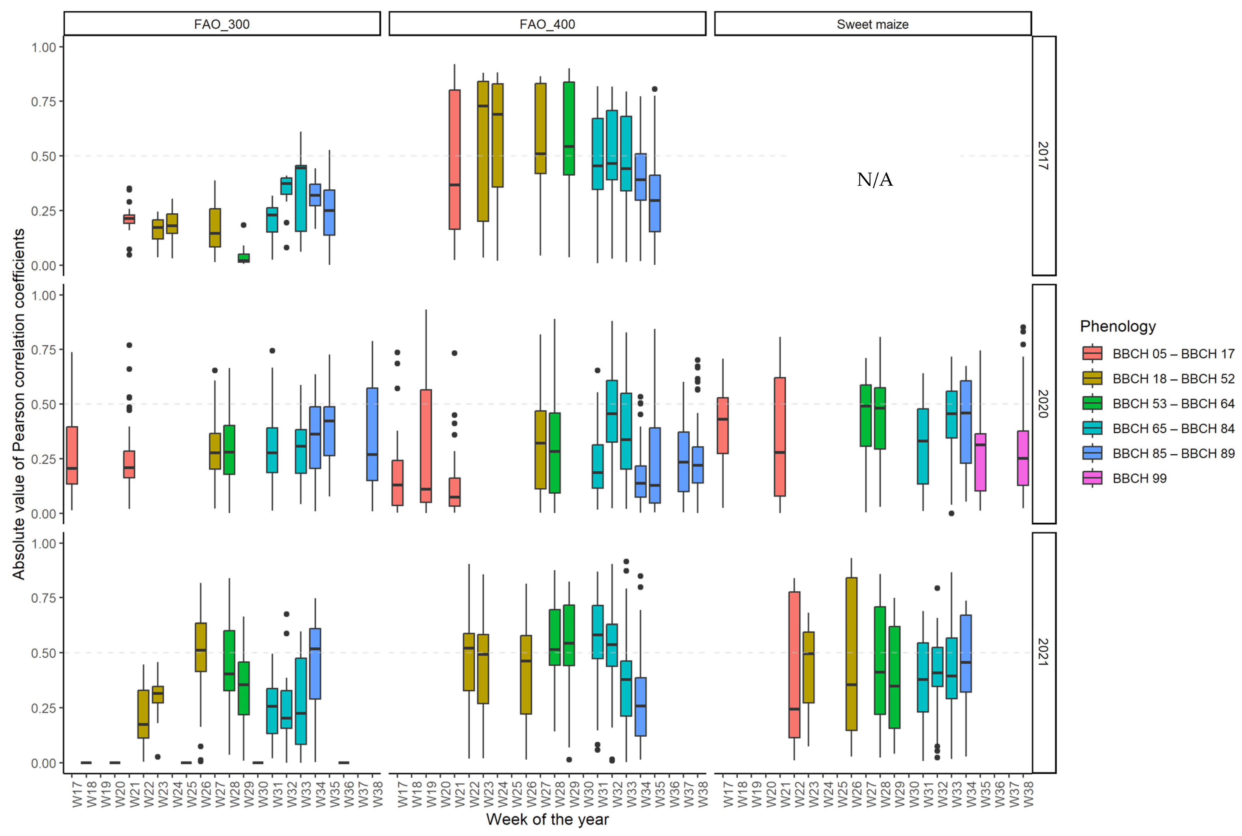
3.5. The Optimal Maize Phenology for Cotton Bollworm Surveillance

Not all maize phenological phases were suitable for the CBW damage surveillance because the PCCs differ remarkably between the groups of the BBCH stages. The PCCs were low in the early phenological phases (before canopy closure) of the sweet, mid–early, and mid–late grain maize hybrids, considering each band and the VIs. In the late (physiological maturation) phenological phases of the mid–late (FAO 400) maize hybrids, consistently low PCCs were exhibited, regardless of the chosen band or VI (Figure 10). The recordings of the BBCH stages included the most important phenological groups. Due to the lack of weekly cloud-free satellite images, a more precise analysis is not possible within the scope of this study. Humid weather conditions reduced the correlation strength.

Means, medians, and standard deviations of the absolute values of the PCCs were analyzed and grouped by the weeks of the year, year, maize cultivation purpose, and maturity group. Means and medians were close to each other within each category. The mean of the absolute values of the PCCs in each week of the early phenological phase (BBCH 05–BBCH 17) were mainly around 0.25 in the grain maize fields (the PCC means of mid–early hybrids ranged from 0.11 to 0.27, and the PCC means of mid–late hybrids ranged from 0.13 to 0.46) and were between 0.35 and 0.39 in the sweet maize fields.

The PCC means after the canopy closure to the harvest (BBCH 18–BBCH 98) ranged from 0.38 to 0.47 for the sweet maize fields, but other weeks that were be not suitable for CBW surveillance could not be distinguished. In the mid–early (FAO 300) grain maize fields, the weekly mean of all the PCCs after the canopy closure ranged from 0.16 to 0.50 (except for one week in 2017, where the PCC mean was 0.04).

The highest values in these fields were reached during ripening (BBCH 85–BBCH 89), ranging from 0.24 to 0.43 (Figure 10). In the mid–late (FAO 400) grain maize hybrids, the weekly average of the PCCs ranged from 0.23 to 0.6 (mostly around 0.5) from the canopy closure to the end of grain filling (BBCH 18–BBCH 84). However, during ripening and senescence, the average of the PCCs’ strength falls to between 0.18 and 0.38.

Generally, the correlation strength in the mid–late (FAO 400) grain maize group was higher than in both other groups (Figure 10). For the comparison of seasonality effect, the PCCs were found to be stronger in the two arid years (2017 and 2021) than in the humid year (2020) for the grain maize fields. The average strength of the PCCs for the sweet maize fields were not different year by year, as these fields were irrigated.

In summary, the early period of maize development (before canopy closure) was inappropriate for CBW larval damage surveillance in each group of maize hybrids. Moreover, the correlations were weak in the late-ripening period of the mid–late maize hybrids, contrary to the sweet maize and mid–early hybrids. Therefore, the time period that is found to be sufficient for the surveillance of damage (considering the maize phenological phases and the dependence on maize cultivation purpose and maturity group) will be referred to as the Digital Evaluation Period of CBW damage (DEPC) in the following sections.

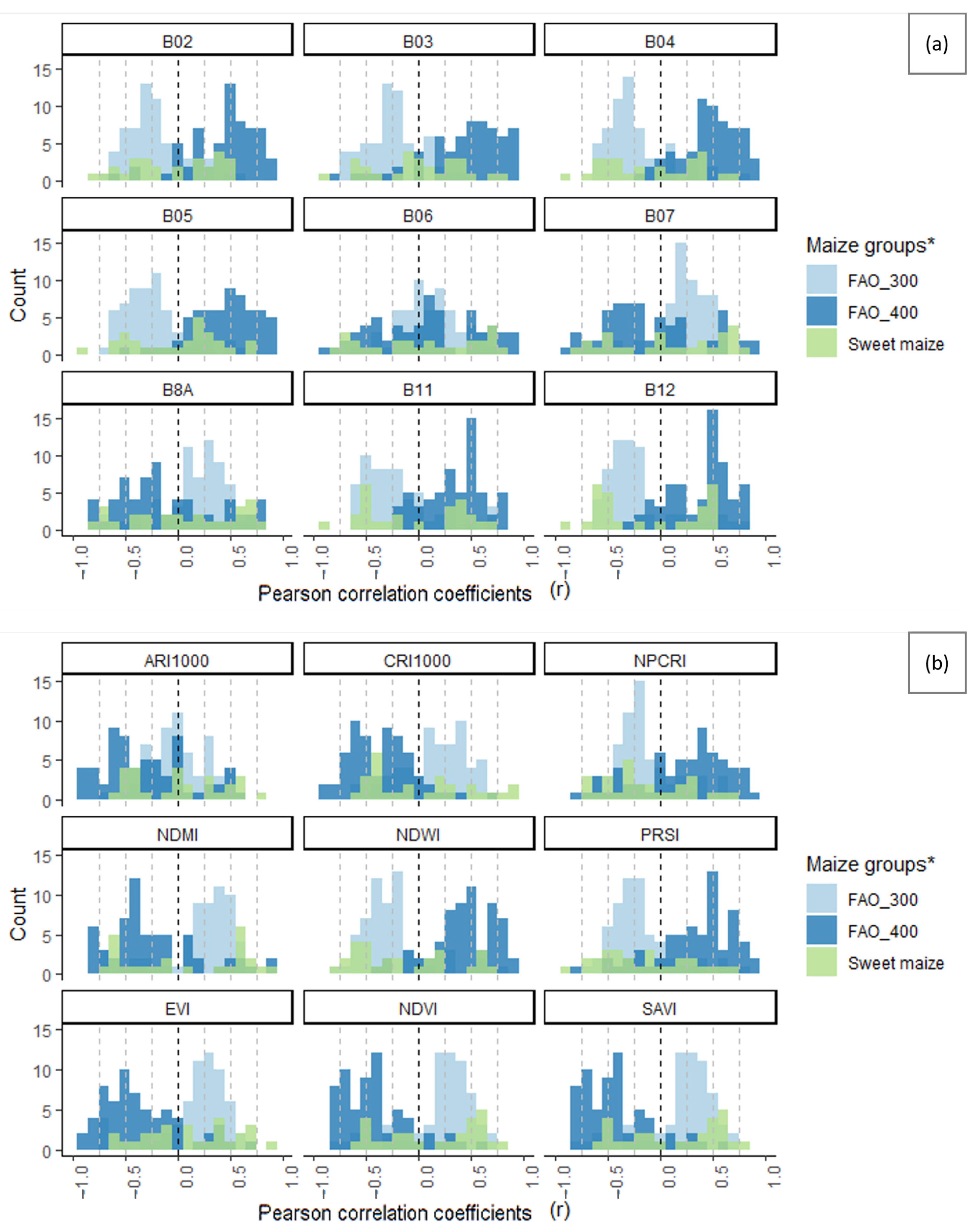
3.6. Suitability of Different Spectral Bands and Vegetation Indices for Cotton Bollworm Surveillance

To ascertain the optimal band or index for surveillance, an analysis was conducted on the mean, standard deviation (SD), median, and maximum frequency of the PCCs associated with each band and VI, focusing on the DEPC (Figure 11 and

Table 6. Mean, median, and standard deviation (SD) of the Pearson correlation coefficients of ear damage of cotton bollworm larvae with spectral bands of Sentinel-2 and vegetation indices (Green color highlights the most suitable bands and indices for surveillance of cotton bollworm damage).

	Band/Index	Mid–Early Grain Maize (FAO 300 Group)			Mid–Late Grain Maize (FAO 400 Group)			Sweet Maize
		Mean	Median	SD	Mean	Median	SD	Mean	Median	SD
Visible bands	B02	−0.21	−0.28	0.28	0.44	0.51	0.33	−0.06	0.00	0.42
	B03	−0.23	−0.27	0.27	0.42	0.50	0.39	−0.01	0.02	0.43
	B04	−0.21	−0.30	0.32	0.46	0.49	0.27	−0.09	−0.22	0.44
Red-edge bands	B05	−0.23	−0.26	0.30	0.44	0.50	0.31	−0.02	0.06	0.43
	B06	0.08	0.06	0.31	0.07	0.07	0.49	0.05	0.07	0.53
	B07	0.18	0.23	0.30	−0.10	−0.18	0.46	0.08	0.05	0.53
NIR band	B8A	0.18	0.23	0.29	−0.09	−0.20	0.46	0.08	0.07	0.52
SWIR bands	B11	−0.20	−0.27	0.33	0.34	0.39	0.28	−0.06	−0.16	0.49
	B12	−0.20	−0.29	0.34	0.38	0.49	0.29	−0.14	−0.41	0.50
Pigment-based VIs	ARI	0.02	0.02	0.28	−0.28	−0.33	0.41	0.03	0.03	0.43
	CRI	0.16	0.17	0.31	−0.35	−0.35	0.32	0.04	−0.06	0.48
	NPCRI	−0.15	−0.21	0.30	0.21	0.33	0.43	−0.13	−0.23	0.41
Water-based VIs	NDMI	0.21	0.28	0.34	−0.22	−0.35	0.43	0.09	0.15	0.55
	NDWI	−0.25	−0.28	0.32	0.43	0.46	0.30	−0.16	−0.27	0.47
General VIs	EVI	0.17	0.25	0.32	−0.34	−0.44	0.37	0.14	0.13	0.42
	NDVI	0.22	0.28	0.33	−0.41	−0.45	0.33	0.16	0.34	0.47
	SAVI	0.22	0.28	0.33	−0.41	−0.45	0.33	0.16	0.34	0.47
Senescence	PSRI	−0.17	−0.25	0.32	0.33	0.42	0.38	−0.15	−0.24	0.43

). The mid–late (FAO 400) hybrids’ PCC means and medians were generally more robust than the mid–early (FAO 300) hybrids, regardless of the selected band or VI.

This study suggests that the bands in the visible spectrum are the most appropriate for the surveillance of damage in grain maize fields, including both maturity categories. The following bands and VIs showed relatively strong PCCs in both sweet and grain maize fields: B12, NDWI, NDVI, and PSRI. The suitability of the EVI and SAVI for damage surveillance were satisfactory, although the usability of the NDVI surpassed the usability of the EVI. Furthermore, the NDVI and SAVI have identical PCCs in the DEPC. Consequently, the SAVI and EVI do not offer any supplementary information compared to the NDVI.

In the case of grain maize fields, the medians of the PCCs show greater strength compared to the means. The medians demonstrated a greater proximity to the peak of the histogram. In the case of grain maize, visible bands (namely B02 (blue), B03 (green), and B04 (red)) had the highest average and medians of the PCCs (Table 6). The histogram peaks in these bands emerge at stronger correlation values compared to all other bands and VIs within one maturity group. This observation is valid for both the mid–early and mid–late hybrids, as the peaks were around −0.3 (mid–early: FAO 300) and +0.5 (mid–late: FAO 400) (Figure 11a). In the FAO 300 maturity group, the distribution of PCCs of the visible bands was predominantly in the negative range, whereas in the FAO 400 hybrids, the distribution shifted towards the positive range.

In the case of the grain maize fields, the B05 had a relatively uniform distribution of PCCs in the positive range for FAO 400 and in the negative range for FAO 300 maturity group. This band had stronger PCCs than the other red-edge bands (B06 and B07). The suitability of B06 and B07 for CBW monitoring was unsatisfactory. Means, medians, and histogram peaks consistently approached zero (Table 6 and Figure 11a). The distribution of the PCCs in these bands exhibited a near equal occurrence of negative and positive values. The near-infrared (NIR) band, namely band B8A, has a low average PCC. The near-infrared (NIR) band in the FAO 400 category shows an especially high standard deviation. The SWIR bands (B11 and B12) show the highest peak of PCC values (the highest number of PCCs equal to the histogram peak). These PCC values were among the strongest observed across all histogram peaks. In the case of the FAO 400 maturity group, both B11 and B12 have a peak at +0.50, but in case of the FAO 300 hybrids, B12 has peaks at −0.30 and −0.40, whereas B11 had a peak at −0.50, which was the most prominent peak among all bands and VIs in the FAO 300 maize fields (Figure 11a).

The pigment-related VIs of the grain maize fields, including the ARI, CRI, and NPCRI, are unsuitable for damage surveillance. The means and medians of their PCCs were weak, while the standard deviations were observed to be extensive (Table 6). Additionally, the histogram peaks were around zero for both maturity groups (Figure 11b). The suitability of the general vegetation indices (the EVI, NDVI, and SAVI) for the surveillance of CBW larval damage was favorable in both maturity groups of grain maize. The means and medians of these VIs were slightly inferior compared to the visible bands. The NDVI and SAVI exhibited identical PCC values in the DEPC. Consequently, both indices had equivalent medians, means, and distributions. The NDVI shows stronger PCC means and medians compared to the EVI in both maturity groups of grain maize (Table 6). Although, using the EVI, the PCCs have histogram peaks at stronger correlation values, the count of the stronger PCCs of the NDVI was higher (Figure 11b). The moisture-related VIs (the NDMI and NDWI) show relatively strong mean and median PCCs compared to other VIs in both maturity groups. In the FAO 400 hybrids, only the NDWI shows a significant correlation (Table 6).

In sweet maize fields, PCC means and medians of most spectral bands were around zero, except for the B12 (SWIR) band, where the median was −0.41, which was the strongest median among all bands and VIs (Table 6). Pigment-related VIs (the ARI, CRI and NPCRI) are unsuitable for damage surveillance in sweet maize fields, as the means and medians of the PCCs were low, and the histogram peaks were around zero. General VIs (the EVI, NDVI, and SAVI) showed a relatively good suitability for damage surveillance, similarly to grain maize. The mean PCCs were slightly weaker, and the median PCCs were stronger than in the FAO 300 hybrids. The NDVI and SAVI exhibited the same PCC values from canopy closure, and therefore also exhibited identical medians, means, and PCC distributions, similarly to grain maize (Table 6, Figure 11). The NDVI surpassed the EVI. Moisture-related vegetation indices (NDMI, NDWI) were different from each other. The NDMI did not perform well. However, the NDWI had one of the strongest mean and median PCCs among bands and VIs (Table 6).

The week of the year is an important influencing factor of the strength of the PCCs of a particular band or vegetation index (as the weather conditions of different years were highly different, and phenology was already found to be important). Therefore, a linear model was fit with the PCCs as the dependent variable and the week of the year as the independent variable, and the three years were separately analyzed (Figure 12,

Table A2. Linear model of Pearson correlation coefficients (PCCs) between ear damage caused by cotton bollworm and surface reflectance measured on each spectral band of Sentinel-2, and vegetation indices calculated from reflectance values, as a dependent variable of time (week of the year). Linear models were fitted on coefficients of each combination of year, maize type, and band/vegetation index. (x = week of the year, x = [DEPC], y = Pearson correlation coefficient, *—significant R² at p < 0.05).

		FAO 300 Grain Maize Fields				FAO 400 Grain maize Fields				Sweet Maize Fields
Year	Band/ Index	Equation	R2	p		Equation	R2	p		Equation	R2	p
2017	B02	y = −0.03 x + 0.99	0.51	0.02	*	y = 0.01 x + 0.07	0.01	0.69		n/a	n/a	n/a
2020	B02	y = −0.01 x − 0.05	0.04	0.25		y = 0 x + 0.27	0.00	1.00		y = 0 x + 0.16	0.00	0.99
2021	B02	y = −0.04 x + 0.99	0.15	0.10		y = 0.02 x − 0.07	0.20	0.02	*	y = 0.04 x − 1.4	0.11	0.23
2017	B03	y = −0.02 x + 0.66	0.32	0.09		y = 0.02 x − 0.39	0.02	0.62		n/a	n/a	n/a
2020	B03	y = −0.01 x − 0.12	0.02	0.41		y = 0.02 x − 0.3	0.03	0.48		y = 0 x + 0.21	0.00	0.92
2021	B03	y = −0.02 x + 0.34	0.04	0.42		y = 0.02 x + 0.15	0.10	0.10		y = 0.06 x − 1.75	0.17	0.13
2017	B04	y = −0.04 x + 1	0.73	0.00	*	y = 0.02 x + 0.1	0.03	0.55		n/a	n/a	n/a
2020	B04	y = −0.01 x + 0	0.06	0.19		y = 0.02 x − 0.31	0.04	0.39		y = 0.03 x − 0.8	0.03	0.56
2021	B04	y = −0.03 x + 0.89	0.08	0.23		y = 0.02 x − 0.01	0.16	0.04	*	y = 0.06 x − 2	0.22	0.08
2017	B05	y = −0.03 x + 0.75	0.43	0.04	*	y = 0.02 x − 0.16	0.03	0.57		n/a	n/a	n/a
2020	B05	y = −0.02 x + 0.18	0.11	0.07		y = 0.01 x + 0.08	0.00	0.76		y = 0 x + 0.14	0.00	0.98
2021	B05	y = −0.03 x + 0.74	0.09	0.22		y = 0.01 x + 0.25	0.07	0.18		y = 0.07 x − 2.18	0.24	0.06
2017	B06	y = 0.05 x − 1.27	0.53	0.02	*	y = −0.03 x + 0.81	0.02	0.60		n/a	n/a	n/a
2020	B06	y = −0.01 x + 0.4	0.02	0.47		y = 0.06 x − 1.87	0.16	0.06		y = −0.03 x + 0.63	0.02	0.66
2021	B06	y = 0.05 x − 1.37	0.24	0.03	*	y = −0.08 x + 2.52	0.43	0.00	*	y = 0.08 x − 2.24	0.37	0.02	*
2017	B07	y = 0.04 x − 1.1	0.41	0.04	*	y = −0.05 x + 1.26	0.16	0.15		n/a	n/a	n/a
2020	B07	y = −0.01 x + 0.56	0.04	0.26		y = −0.01 x + 0.12	0.01	0.67		y = −0.02 x + 0.42	0.01	0.76
2021	B07	y = 0.04 x − 1.05	0.13	0.13		y = −0.1 x + 2.73	0.55	0.00	*	y = 0.07 x − 1.95	0.31	0.03	*
2017	B8A	y = 0.05 x − 1.23	0.47	0.03	*	y = −0.06 x + 1.51	0.24	0.07		n/a	n/a	n/a
2020	B8A	y = −0.01 x + 0.47	0.02	0.48		y = −0.01 x + 0.13	0.01	0.66		y = −0.03 x + 0.62	0.02	0.67
2021	B8A	y = 0.04 x − 1.14	0.18	0.07		y = −0.09 x + 2.69	0.55	0.00	*	y = 0.08 x − 2.09	0.33	0.02	*
2017	B11	y = −0.03 x + 0.96	0.53	0.02	*	y = 0.01 x + 0	0.02	0.63		n/a	n/a	n/a
2020	B11	y = −0.01 x − 0.03	0.04	0.27		y = −0.01 x + 0.61	0.01	0.59		y = 0.03 x − 0.67	0.03	0.60
2021	B11	y = −0.04 x + 1.05	0.10	0.21		y = 0.03 x − 0.36	0.22	0.02	*	y = 0.06 x − 1.86	0.14	0.21
2017	B12	y = −0.04 x + 0.99	0.53	0.02	*	y = 0.01 x + 0.1	0.03	0.57		n/a	n/a	n/a
2020	B12	y = −0.01 x − 0.07	0.04	0.30		y = 0.01 x + 0.1	0.00	0.82		y = 0.04 x − 1.03	0.04	0.51
2021	B12	y = −0.05 x + 1.36	0.16	0.09		y = 0.03 x −0.56	0.25	0.01	*	y = 0.01 x − 0.77	0.01	0.68
2017	ARI	y = 0.01 x − 0.35	0.04	0.56		y = 0 x −0.2	0.00	0.99		n/a	n/a	n/a
2020	ARI	y = 0.03 x − 1.04	0.19	0.06		y = −0.06 x + 1.57	0.14	0.08		y = 0.01 x − 0.43	0.01	0.78
2021	ARI	y = −0.03 x + 0.78	0.11	0.17		y = −0.01 x − 0.1	0.05	0.27		y = −0.04 x + 1.23	0.07	0.34
2017	CRI	y = 0.03 x − 0.98	0.56	0.01	*	y = 0.01 x − 0.79	0.03	0.57		n/a	n/a	n/a
2020	CRI	y = 0.01 x − 0.2	0.06	0.19		y = 0.01 x − 0.37	0.00	0.82		y = 0.01 x − 0.56	0.01	0.80
2021	CRI	y = 0.05 x −1.24	0.18	0.07		y = −0.05 x + 0.98	0.41	0.00	*	y = 0 x + 0.18	0.00	0.98
2017	NPCRI	y = −0.02 x + 0.26	0.32	0.09		y = 0.01 x + 0.38	0.01	0.68		n/a	n/a	n/a
2020	NPCRI	y = 0 x −0.38	0.00	0.75		y = 0.01 x + 0.07	0.00	0.88		y = 0.04 x − 1.26	0.09	0.35
2021	NPCRI	y = −0.02 x + 0.8	0.07	0.26		y = 0.06 x − 1.58	0.23	0.01	*	y = 0.03 x − 1.14	0.06	0.39
2017	NDMI	y = 0.04 x − 1.2	0.48	0.03	*	y = −0.04 x + 0.84	0.20	0.11		n/a	n/a	n/a
2020	NDMI	y = 0.01 x + 0.19	0.02	0.46		y = −0.01 x − 0.16	0.00	0.84		y = −0.01 x + 0.28	0.00	0.83
2021	NDMI	y = 0.05 x − 1.45	0.18	0.09		y = −0.11 x + 3.05	0.60	0.00	*	y = 0.08 x − 2.02	0.26	0.07
2017	NDWI	y = −0.05 x + 1.38	0.66	0.00	*	y = 0.01 x + 0.35	0.01	0.76		n/a	n/a	n/a
2020	NDWI	y = −0.01 x − 0.15	0.02	0.42		y = 0.01 x − 0.02	0.02	0.58		y = 0.03 x − 0.73	0.02	0.66
2021	NDWI	y = −0.03 x + 0.74	0.07	0.28		y = 0.05 x − 1	0.32	0.00	*	y = −0.02 x + 0.17	0.04	0.47
2017	EVI	y = 0.03 x − 0.61	0.44	0.04	*	y = 0 x − 0.52	0.00	0.90		n/a	n/a	n/a
2020	EVI	y = 0.02 x − 0.22	0.12	0.06		y = −0.02 x + 0.25	0.01	0.63		y = −0.03 x + 0.97	0.05	0.50
2021	EVI	y = 0.03 x − 0.87	0.07	0.29		y = −0.05 x + 1.09	0.24	0.01	*	y = −0.01 x + 0.52	0.01	0.80
2017	NDVI	y = 0.04 x −1.02	0.60	0.01	*	y = 0 x − 0.61	0.00	0.94		n/a	n/a	n/a
2020	NDVI	y = 0.01 x + 0.13	0.03	0.37		y = −0.02 x + 0.38	0.04	0.36		y = −0.03 x + 0.74	0.02	0.64
2021	NDVI	y = 0.04 x − 1.02	0.10	0.20		y = −0.06 x + 1.21	0.31	0.00	*	y = 0 x + 0.48	0.00	0.88
2017	SAVI	y = 0.04 x − 1.02	0.60	0.01	*	y = 0 x − 0.61	0.00	0.94		n/a	n/a	n/a
2020	SAVI	y = 0.01 x + 0.13	0.03	0.37		y = −0.02 x + 0.38	0.04	0.36		y = −0.03 x + 0.74	0.02	0.64
2021	SAVI	y = 0.04 x − 1.02	0.10	0.20		y = −0.06 x + 1.21	0.31	0.00	*	y = 0 x + 0.48	0.00	0.88
2017	PRSI	y = −0.03 x + 0.75	0.49	0.02	*	y = 0 x + 0.64	0.00	0.92		n/a	n/a	n/a
2020	PRSI	y = −0.01 x + 0.01	0.04	0.27		y = 0.01 x − 0.05	0.00	0.76		y = 0.03 x − 0.83	0.03	0.59
2021	PRSI	y = −0.03 x + 0.96	0.08	0.24		y = 0.07 x −1.8	0.44	0.00	*	y = 0.02 x − 0.94	0.03	0.52

). Only the DEPC was considered in each year. Overall, the R² of the linear models covered a wide range (from 0 to 0.73).

For the grain maize fields, the linear models of the different bands and VIs were similar to each other in the two arid years (2017 and 2021): the slope of the linear models was the same or closer to each other than in the humid year (2020). Moreover, the R² of the models reached a higher value in the arid years than in the humid year. The maximum R² in the two arid years were 0.73 and 0.60, respectively, while in the humid year of 2020, the maximal R² was 0.19.

This trend was not observed in sweet maize as only two years were analyzed: a rainy and cool (2020) and an arid and hot (2021) year. Moreover, the sweet maize fields were irrigated. In 2020, there was no band or VI where the relationship between the weeks and PCCs was significant, regardless of the maize hybrid. There was a significant linear relationship between the PCCs of almost all bands or VIs and the weeks of the DEPC of 2017 in the FAO 300 hybrids, and the DEPC of 2021 in the FAO 400 hybrids (Table A2).

The highest four R² values (above 0.60) were found in 2017 in the FAO 300 category: B04, NDWI, NDVI, and SAVI (R² = 0.73, 0.66, 0.60, and 0.60, respectively), and in 2021 in the FAO 400 category: NDMI (R² = 0.60, Table A2). The slope of the linear models of the different years was similar in the visible bands (B02, B03, B04) and in one of the red-edge bands (B05) in the FAO 400 category, and in B03, B05, and EVI in the FAO 300 category. The slope of the model of the B03 band each year was around 0.2 in both grain maize maturity groups. These results highlight that the visible bands not only reach the highest PCCs but also seem to give the most reliable estimations throughout the different years for commercial grain maize.

4. Discussion

In this study, satellite imagery was analyzed for the surveillance of damage by CBW larvae to maize ears. The study hypothesized that reflectance represents changes in the maize and visual stimuli that play a significant role in CBW adult oviposition preference. CBW larvae do not change hosts during the larval stage; therefore, their most probable locations are the CBW adult’s preferred host, highlighting potential locations for larvae damage. Therefore, there is a near-optimal combination of satellites, spectral bands, vegetation indices (VIs), and temporal resolutions for the best possible surveillance of damage by CBW larvae. This combination should function under a variety of agronomic and weather conditions.

The analysis of the CBW damage distribution was conducted in an uncontrolled agricultural setup. The selection of sampling zones was based on a methodology that aimed to include various maize features. As well as the condition of the plants, the ear damage distribution of the damaged ears showed high variability in all observed fields across the years. The within-field variability of the damaged ears was also high. Although the weather conditions of the sampled years differed, the percentage of ears damaged in all the fields was similar. This result suggests the counteracting influence of several factors, such as weather, location, field heterogeneity, and maize hybrid, since the variability in the damage distribution within each field and farm was considerable.

Pearson correlation coefficients (PCCs) were calculated to assess the relationship between the percentage of damaged ears and surface reflectance along with the various VIs derived from spectral bands of the Landsat 8 and Sentinel-2 satellites. This analysis considered the percentage of CBW-damaged ears observed in the sampling zones within each field. Satellite images were collected in the best available temporal resolution (based on the available cloud-free satellite images of the fields).

The PCCs were diverse, ranging from no correlation to a correlation as high as |r| = 0.93 (both positive and negative). The absence of correlation coefficients beyond 0.95 suggests that besides satellite imagery, other factors should be considered during CBW surveillance in maize fields.

No statistically significant difference was observed in the performance of the Landsat 8 and Sentinel-2 multispectral satellites when evaluating each spectral band and VI. These results suggest that the disparity in the spectral characteristics of the two multispectral satellites was not the primary distinguishing feature when comparing the suitability of the satellites for CBW surveillance. Nevertheless, the Sentinel-2 satellite shows stronger maximum as well as minimum PCCs across nearly all spectral bands and VIs. The application of Sentinel-2 is furthermore advantageous due to the availability of more cloud-free recordings, and its shorter orbiting period supports the more frequent monitoring of important phenological phases. A comprehensive evaluation of the Landsat 8 and Sentinel-2 satellites has been conducted in many fields of agriculture, revealing similar results. The two satellites showed comparable accuracy in LAI prediction [106]. Sentinel-2 only slightly surpassed Landsat 8 in land-use classification [107,108,109], yield prediction [110,111], monitoring of damages to forest ecosystems, such as burnt areas [112], or pest distribution analysis, e.g., the European spruce bark beetle (Ips typographus L.) [113].

Unexpectedly, the first attempt to find the most correlated band and VI with CBW damage was unsuccessful, as there were no statistically significant differences between the bands (even when examining the absolute values of the PCCs), and no VI could be identified that would perform better than the others. The PCCs within a group (belonging to a band or VI) highly varied, and no consistent patterns of PCCs were found. To assess the inconsistency, a cluster analysis was conducted.

The PCCs were similar in 2017 and 2021 (arid years) but different in 2020 (humid year). The cluster analysis endorsed yearly differences, as most Cluster 1 points belonged to 2017. In 2020, the PCCs were weaker than in the other two years, regardless of the observed spectral band, index, maize cultivation purpose, or maturity group. However, contrary to the arid years, two CBW generations could damage the maize ears in 2020. Significant differences were observed between the PCCs of sweet maize and grain maize hybrids. However, grouping by years contributed, but did not explain the inconsistency of the PCCs.

The most prominent explanation for the inconsistency of the PCCs is that the different grain maize maturity groups showed correlations in opposite directions. The separation of different maturity groups of grain maize hybrids was achieved through clustering. Most of Cluster 5 was associated with the FAO 300 maize hybrids, while the other clusters (Cluster 1–4) were predominantly associated with the FAO 400 maize hybrids. The two maturity groups of grain maize fields show patterns of PCCs with opposite signs, particularly in the visible spectrum (B02, B03, and B04—blue, green, and red, correspondingly), the short-wave infrared (SWIR) range, and all examined vegetation indices. The positive PCCs of mid–late (FAO 400) hybrids were primarily observed in the visible spectrum B02, B03, B04, and B05, as well as in the SWIR bands (B11 and B12), and some indices, namely the NDWI, PCRI, and PRSI. Conversely, the PCCs of the mid–early (FAO 300) hybrids in these bands and VIs were predominantly negative. When the PCCs of the mid–late maize hybrids were found to be negative, namely in B07, the NIR band (B8A), as well as general vegetation indices (the EVI, NDVI, and SAVI), the normalized difference moisture index (NDMI), mid-early maize hybrids showed positive PCCs. The suitability of remote sensing for the surveillance of damage from CBW larvae was better in the FAO 400 grain maize maturity group than in the FAO 300 group, as the PCCs of the FAO 400 hybrids were stronger each year, regardless of the chosen spectral band or index.

The main reason for the unexpectedly varying correlations (with correlation coefficients of different signs) of different grain maize maturity groups may be attributed to the subtle differences in their spectral profiles and the small temporal shifts in their reflectance patterns (Figure A2, Figure A3, Figure A4), which are aligned with differences in their phenological states when the CBW adults appears in the field (Figure 5). If the adult faces different phenological phases of maize during oviposition, the viability of the eggs and larvae can vary depending on the limiting factors during that specific phenological phase.

Our results are supported by studies which suggest that maize’s spectral profile can be used to distinguish different maize varieties and hybrids [54]. Studies have identified variations in the spectral profile of distinct maize groups, leading to disparities in the effectiveness of remote sensing for detecting or predicting specific objectives. For example, the accuracy of the estimation of leaf chlorophyll content through remote sensing was improved by deriving separate calibration equations for each maize type [114]. It was found that the canopy reflectance of maize fields had a different efficacy for estimating leaf nitrogen content and yield, when the maize hybrids were grouped by the efficiency of nitrogen utilization [115]. Moreover, remote sensing is an increasingly popular tool for maize phenotyping and breeding, as the spectral properties of different maize varieties can detect genetic differences [116,117,118]. The difference between the two grain maize categories can be recognized by the level of damage percentages, as it was higher in the FAO 400 category than in the FAO 300 category.

There were substantial variations in the PCCs among different groups of BBCH stages. Certain phenological phases consistently showed low PCCs, regardless of the selected band or VI. However, the outcome was contingent upon the maize cultivation purpose, maturity group, and the prevailing weather conditions of the years.

The mean PCCs between phenological phases were consistently lower during the early stages (from emergence until canopy closure) compared to other stages in sweet maize, as well as in mid–early and mid–late grain maize hybrids, as expected. The physiological maturation and senescence phases show consistently low PCC values within the mid–late hybrids. However, this late phenology within the mid–early grain and sweet maize hybrids could not be excluded, as the PCCs in this period were as high as after the canopy closure.

Hence, the period with stronger PCCs was observed, suggesting that phenological phases specific to maize cultivation purpose and maturity group are observed, referred to as the Digital Evaluation Period of CBW damage (DEPC). Several studies have identified specific phenological phases of maize that surpassed others when remote sensing was used to estimate different aspects of maize fields. Studies revealed that the strongest correlations of maize canopy reflectance and VIs with yield, dry matter weight, leaf nitrogen content, and leaf chlorophyll content were observed in the filling stage of maize [115]. For maize yield prediction, a combination of tasseling, silking, milking, and ripening phenological phases was the most suitable [119]. In contrast, others revealed the maximal correlation with yield three months after sowing [120,121].

Based on the literature, the highest correlations were expected in the silking and tasseling phenological phases. It was unexpected that the correlations were not lower at a vegetative phenological phase (namely after canopy closure, BBCH18-52) than during silking and tasseling (BBCH53-64). This highlights the potential of the mid-term forecasting of CBW damage distribution before the pest has even appeared in the field.

This study suggests that the visible bands (B02, B03, and B04) are the most appropriate for the surveillance of CBW larval ear damage in grain maize fields, including both maturity groups. While most multispectral-based remote sensing research uses only VIs, visible bands were found to be more suitable in our research. These results are supported by studies revealing the sensitivity of CBW adults for blue and green [34,35]. These results also highlight the importance of incorporating spectral band-measured reflectance values directly into CBW damage surveillance models, similarly to some yield prediction research [121,122]. Although each visible band was well-suited, there was no considerable difference among the colors, contrary to the studies revealing CBW adults’ preference for particular colors [36,37,38]. Even though B02, B03, and B04 reached the highest mean PCCs, the strength of the mean PCCs remained moderate, and the variation within the PCCs were relatively high. Therefore, the visual stimuli and the color preference of CBW for oviposition and the subsequent larval damage were found to have considerable effects but were not the most dominant factors. This indicates that CBW female adults prefer hosts (later larvae damage) based on a complex stimuli (e.g., olfactory), supporting studies that emphasize the importance of kairomones and volatiles [123,124,125].

The bands and VIs that demonstrated consistent relatively good fitness in both sweet maize and grain maize fields were as follows: the B12 (SWIR) band, NDWI, NDVI, and PSRI. The correlation of the EVI and SAVI was satisfactory, while the NDVI surpassed the EVI. Furthermore, the NDVI shows identical PCCs as the SAVI, offering no supplementary information beyond the NDVI. Low to strong, mainly negative correlations were found with the SWIR bands in mid–early (FAO 300) hybrids. If the reflectance of the maize canopy is higher in the SWIR spectral region, it may indicate that the leaves contain a lower proportion of water [126]. Our study suggests that there is a relationship between the maize canopy reflectance in the SWIR spectral region and the CBW larval damage. This suggests that a higher water content in the leaves can affect the damage level in maize. This indication is supported by studies suggesting that water-stressed leaves were less preferred by the CBW [88,127]. The NDMI results also support this conclusion, as mainly positive correlations were found in the FAO 300 maturity group. Therefore, in the FAO 300 hybrids, the moisture of plants was found to be an important factor in CBW larval damage since these hybrids are already in a later phenological stage when the pests appear. The mid–late (FAO 400) hybrids showed low to strong positive correlations in the SWIR ranges and negative correlations with the NDMI. This finding indicates that in the FAO 400 category, the maturity of the maize plants is more important than water content, as the swarming peaks and subsequent oviposition and larval feeding occur at an earlier phenological phase of the maize plants (as shown by the results with the general VIs, where mostly negative correlations were found in the FAO 400 maturity group of grain maize).

4.1. Limitations and Uncertainties

The analysis holds limitations and uncertainties in some respects, mainly concerning the limitations of the methodology and dataset and consequently the transferability to other regions and hosts.

The collection of data was limited to the Carpathian Basin. The Carpathian Basin’s climatic conditions are temperate, and this climate does not permit the continuous presence of the CBW in this region (although, it should be noted that overwintering is becoming more frequent here [7]). Temperature is the most significant factor determining the moth development rate [21,128], and the CBW in this region develops two to four generations, in contrast to the subtropical regions where the number of moth generations can reach more than ten [128]. For this reason, the extension of the method to the Mediterranean regions requires further investigation. Thus, at present, the results can only be interpreted within temperate climatic regions.

An important limitation with respect to the data concerns the host plants. This study’s data collection was restricted to maize cultivars, encompassing non-Bt, early, and mid-maturing hybrids. The approach demonstrated in this research is likely to be maize-specific or applicable to cultivars with similar growth cycles. In areas where Bt maize is also cultivated, this approach could be even more valuable, since it enables us to identify locations where resistant CBW generations are most likely to cause damage, thus providing another early monitoring and intervention point after the resistant adults have been controlled.

One further limitation with respect to the dataset is that the phenological observations were restricted to the most significant phenology groups, so if there is a particular phenology within these periods that has achieved a consistently high level of correlation, it will not stand out.

Although the maize maturity group and the main phenology groups explained the primary characteristics of the PCCs of a field, the PCCs still have a variability within the different categories and phenological groups. Results could be improved by observing the exact silking dates of the hybrids and analyzing their coincidence with the CBW adult flight peak with daily accuracy. Further subcategories may enhance the usability of multispectral satellite imagery for CBW damage surveillance, providing additional aspects for research.

The use of satellite technology and the selected satellites also hold some concerns.

The cloud-free coverage of satellite images for each farm and each year at every phenological stage varies and some observations can only be based on thin data density, while others benefit from a more extensive data availability, and some combinations are entirely missing. Therefore, by applying harmonized satellite products of the two satellites, along with more frequent and sampling zone-specific phenological observations, it is possible to identify the optimal CBW damage surveillance period more precisely.

Concerning the spectral bands’ suitability for the surveillance of CBW damage, a limited number of bands were analyzed due to the attributes of the satellite sensors. A higher spectral resolution and the application of a hyperspectral sensor could improve the suitability of the remote sensing imagery for CBW surveillance. Therefore, further research in this area is suggested.

The most important limitation of using multispectral satellite products for CBW surveillance that becomes clear from the results is that it gives no information on the timing of the pest’s appearance in the field. Therefore, the use of multispectral satellite data for CBW surveillance should be combined with traps.

4.2. Outlook

The method presented in this study supports plant protection decisions against the CBW, enabling long-term damage prediction before its appearance. Other models provide information on CBW activity long before the CBW appears in the field. These systems primarily focus on tracking the migration path of adults and the temperature-dependent development of the pest (as written in the Introduction), but not the extent of the expected damage. In contrast, the method presented here specifically concentrates on predicting the location and percentage of damage. The previous models did not support the farmers to make specific decisions regarding their farms, nor did they accurately locate and estimate the percentage of damage. The approach presented here, in combination with other models in the future, could provide global, but precise forecasts for smaller regions, regarding damage.

Current short-term forecasting methods primarily focus on the appearance of pests and rely on trapping, including light and pheromone traps. The remote sensing method studied here does not provide information on the timing of pest emergence; it can, however, provide information on the expected degree of damage and location. Thus, the use of multispectral satellite imagery can be a supplementary technique to trap-based strategies. It may help to optimize trap deployment and provide other supplementary measures for the greater effectiveness and precision of plant protection decisions.

The current crop damage monitoring strategy relies mainly on the visual inspections of farmers and advisors, which is time-consuming and laborious. The proposed method allows us to focus on areas where the greatest damage is expected, thereby reducing the number of monitoring points and optimizing the process.

5. Conclusions

This study investigated the use of Landsat 8 and Sentinel-2 satellite-measured surface reflectance as a tool for the damage surveillance of CBW larvae to maize ears. The hypothesis was that there is an optimal combination of satellites, spectral bands, or vegetation indices for achieving the best possible surveillance of maize ear damage by CBW larvae. The study was conducted in an uncontrolled agricultural setup, with sampling zones selected based on the NDVI. The Sentinel-2 satellite slightly surpassed Landsat 8, due to better data availability. The study highlighted the importance of weather conditions: in humid weather conditions, the suitability of remote sensing for damage surveillance was weaker than in arid weather conditions, regardless of the observed spectral band, index, maize cultivation purpose, and maturity group.

The study found a significant difference in the suitability of remote sensing for CBW surveillance in different maize cultivation purposes and maturation categories. In mid–late hybrids, correlations between surface reflectance, VIs, and maize ear damage by CBW larvae were stronger, regardless of the chosen spectral band or index or weather condition. The different spectral profiles of the grain maize maturation categories could explain the difference.

We suggest considering the maturity groups of maize during CBW surveillance with remote sensing imagery. The early phenological phase of maize growth, prior to the formation of a closed canopy, was found to be unsuitable for the damage surveillance of CBW larvae across different maize cultivation purposes and maturity groups. Late phenological phases in mid–late grain maize hybrids were unsuitable as well. Visible bands considerably surpassed non-visible bands and vegetation indices in grain maize fields, highlighting the importance of incorporating surface reflectance directly into CBW damage surveillance models. The bands and vegetation indices that demonstrated a consistent relatively high correlation in both sweet maize and grain maize fields were as follows: B12 (SWIR band), NDWI, NDVI, and PSRI.

In this study, we established the existence of the relationship and its circumstances between the CBW larval damage in maize and surface reflectance satellite products.

We used only publicly available, cost-free multispectral satellite data for the rapid surveillance of CBW damage in maize over large areas, while using a cost- and labor-effective approach.

Another prominent advantage of the proposed method is that the prediction of damage percentage and location can be made immediately after maize canopy closure, long before the pest appears in the field. The satellite data also provides continuous time sampling and automatic resampling time.

Besides the advantages, it is essential to mention the disadvantages of the method. This method is currently specific to temperate climate areas and maize hosts. Multispectral satellite products do not provide information on the timing of the pest’s appearance; therefore, plant protection interventions cannot rely only on this method.

It is proposed to combine this method with autonomous traps. Once this method is further validated, large areas can be monitored with a reduced number of traps that are precisely located in the areas that are most likely to be damaged. This approach reduces field monitoring points for large areas considering CBW damage.

References

1. Kriticos, D.J.; Ota, N.; Hutchison, W.D.; Beddow, J.; Walsh, T.; Tay, W.T.; Borchert, D.M.; Paula-Moreas, S.V.; Czepak, C.; Zalucki, M.P. The Potential Distribution of Invading Helicoverpa armigera in North America: Is It Just a Matter of Time? PLoS ONE 2015, 10, e0119618. [Google Scholar] [CrossRef]
2. EPPO Global Database. Available online: https://gd.eppo.int/ (accessed on 8 September 2023).
3. Riaz, S.; Johnson, J.B.; Ahmad, M.; Fitt, G.P.; Naiker, M. A Review on Biological Interactions and Management of the Cotton Bollworm, Helicoverpa armigera (Lepidoptera: Noctuidae). J. Appl. Entomol. 2021, 145, 467–498. [Google Scholar] [CrossRef]
4. Szőcs, G.; Tóth, M.; Újváry, I.; Szöcs, G.; Tóth, M.; Ujváry, I.; Szarukán, I. Development of a Pheromone Trap for Monitoring the Cotton Bollworm (Helicoverpa armigera Hbn.) an Upcoming Pest in Hungary. Növényvédelem 1995, 31, 261–266. [Google Scholar]
5. Yadav, S.P.S.; Lahutiya, V.; Paudel, P. A Review on the Biology, Ecology, and Management Tactics of Helicoverpa armigera (Lepidoptera: Noctuidae). Turk. J. Agric.-Food Sci. Technol. 2022, 10, 2467–2476. [Google Scholar] [CrossRef]
6. Lopes, H.M.; Bastos, C.S.; Boiteux, L.S.; Foresti, J.; Suinaga, F.A. A RAPD-PCR-Based Genetic Diversity Analysis of Helicoverpa armigera and H. zea Populations in Brazil. Genet. Mol. Res. GMR 2017, 16, gmr16038757. [Google Scholar] [CrossRef]
7. Keszthelyi, S.; Nowinszky, L.; Puskás, J. The Growing Abundance of Helicoverpa armigera in Hungary and Its Areal Shift Estimation. Cent. Eur. J. Biol. 2013, 8, 756–764. [Google Scholar] [CrossRef]
8. Huang, J. Effects of Climate Change on Different Geographical Populations of the Cotton Bollworm Helicoverpa armigera (Lepidoptera, Noctuidae). Ecol. Evol. 2021, 11, 18357–18368. [Google Scholar] [CrossRef]
9. Virić Gašparić, H.; Vučemilović Jurić, D.; Bažok, R. Assessment of a possible increase in the harmfulness of the cotton bollworm (Helicoverpa armigera Hubner) in Croatia. Entomol. Croat. 2022, 21, 1–9. [Google Scholar] [CrossRef]
10. Yang, L.; Li, M.; Liu, J.; Zeng, J.; Li, Y. Long-Term Expansion of Cereal Crops Promotes Regional Population Increase of Polyphagous Helicoverpa armigera. Available online: https://www.researchsquare.com (accessed on 17 November 2023).
11. Sagar, D.; Nebapure, S.M.; Chander, S. Development and Validation of Weather Based Prediction Model for Helicoverpa armigera in Chickpea. J. Agrometeorol. 2017, 19, 328–333. [Google Scholar] [CrossRef]
12. Keszthelyi, S.; Pál-Fám, F.; Kerepesi, I. Effect of Cotton Bollworm (Helicoverpa armigera Hübner) Caused Injury on Maize Grain Content, Especially Regarding to the Protein Alteration. Acta Biol. Hung. 2011, 62, 57–64. [Google Scholar] [CrossRef] [PubMed]
13. Dömötör, I.; Kiss, J.; Szőcs, G. Coincidence of Silking Time of Corn, Zea mays and Flight Period of Cotton Bollworm, Helicoverpa armigera Hbn.: How Does It Affect Follow-up Abundancy of Larvae on Cobs and Grain Damage in Various Corn Hybrids? Acta Phytopathol. Entomol. Hung. 2009, 44, 315–326. [Google Scholar] [CrossRef]
14. Keszthelyi, S.; Puskás, J.; Nowinszky, L. Light-Trap Catch of Cotton Bollworm, Helicoverpa armigera in Connection with the Moon Phases and Geomagnetic H-Index. Biologia 2019, 74, 661–666. [Google Scholar] [CrossRef]
15. Nowinszky, L.; Puskás, J. Light Trapping of Helicoverpa armigera in India and Hungary in Relation with the Moon Phases. Indian J. Agric. Sci. 2011, 81, 154–157. [Google Scholar]
16. Pan, H.; Xu, Y.; Liang, G.; Wyckhuys, K.A.G.; Yang, Y.; Lu, Y. Field Evaluation of Light-Emitting Diodes to Trap the Cotton Bollworm, Helicoverpa armigera. Crop Prot. 2020, 137, 105267. [Google Scholar] [CrossRef]
17. Nesbitt, B.F.; Beevor, P.S.; Hall, D.R.; Lester, R. Female Sex Pheromone Components of the Cotton Bollworm, Heliothis armigera. J. Insect Physiol. 1979, 25, 535–541. [Google Scholar] [CrossRef]
18. Flórián, N.; Jósvai, J.K.; Tóth, Z.; Gergócs, V.; Sipőcz, L.; Tóth, M.; Dombos, M. Automatic Detection of Moths (Lepidoptera) with a Funnel Trap Prototype. Insects 2023, 14, 381. [Google Scholar] [CrossRef] [PubMed]
19. Duffield, S.J.; Steer, A.P. The Ecology of Helicoverpa Spp. (Lepidoptera: Noctuidae) in the Riverina Region of South-Eastern Australia and the Implications for Tactical and Strategic Management. Bull. Entomol. Res. 2006, 96, 583–596. [Google Scholar] [CrossRef]
20. Narava, R.; Kumar D V, S.R.; Jaba, J.; Kumar P, A.; Rao G V, R.; Rao V, S.; Mishra, S.P.; Kukanur, V. Development of Temporal Model for Forecasting of Helicoverpa armigera (Noctuidae: Lepidopetra) Using Arima and Artificial Neural Networks. J. Insect Sci. 2022, 22, 2. [Google Scholar] [CrossRef]
21. Jallow, M.; Matsumura, M. Influence of Temperature on the Rate of Development of Helicoverpa armigera (Hübner) (Lepidoptera: Noctuidae). Appl. Entomol. Zool. 2001, 36, 427–430. [Google Scholar] [CrossRef]
22. Mironidis, G.K. Development, Survivorship and Reproduction of Helicoverpa armigera (Lepidoptera: Noctuidae) under Fluctuating Temperatures. Bull. Entomol. Res. 2014, 104, 751–764. [Google Scholar] [CrossRef]
23. Mathukumalli, S.R.; Dammu, M.; Sengottaiyan, V.; Ongolu, S.; Biradar, A.K.; Kondru, V.R.; Karlapudi, S.; Bellapukonda, M.K.R.; Chitiprolu, R.R.A.; Cherukumalli, S.R. Prediction of Helicoverpa armigera Hubner on Pigeonpea during Future Climate Change Periods Using MarkSim Multimodel Data. Agric. For. Meteorol. 2016, 228–229, 130–138. [Google Scholar] [CrossRef]
24. Kaneko, S.; Shirotsuka, K.; Shibao, M. Forecast of Peak Dates of Adult Emergence of Helicoverpa armigera in Osaka Prefecture by Using a Simulation Program Based on the Total Effective Temperature Provided by JPP-NET. Annu. Rep. Kansai Plant Prot. Soc. 2017, 59, 105–108. [Google Scholar] [CrossRef]
25. Damos, P.; Papathanasiou, F.; Tsikos, E.; Kyriakidis, T.; Louta, M. Bayesian Non-Parametric Thermal Thresholds for Helicoverpa armigera and Their Integration into a Digital Plant Protection System. Agronomy 2022, 12, 2474. [Google Scholar] [CrossRef]
26. Blum, M.; Nestel, D.; Cohen, Y.; Goldshtein, E.; Helman, D.; Lensky, I.M. Predicting Heliothis (Helicoverpa armigera) Pest Population Dynamics with an Age-Structured Insect Population Model Driven by Satellite Data. Ecol. Model. 2018, 369, 1–12. [Google Scholar] [CrossRef]
27. Jokar, M. A Thermal Forecasting Model for the Overwintering Generation of Cotton Bollworm by Remote Sensing in the Southeast of Caspian Sea. Span. J. Agric. Res. 2022, 20, 1001. [Google Scholar] [CrossRef]
28. Jokar, M.; López-Bernal, Á.; Kamkar, B. The Effect of Spring Flooding on Management and Distribution of Cotton Bollworm (Helicoverpa armigera) by Flood Mapping Using SAR Sentinel-1 and Optical Imagery Landsat-8; a Case Study in Golestan Province, Iran. Int. J. Pest Manag. 2022, 1–11. [Google Scholar] [CrossRef]
29. Kumari, P.; Mishra, G.C.; Srivastava, C.P. Forecasting of Productivity and Pod Damage by Helicoverpa armigera Using Artificial Neural Network Model in Pigeonpea (Cajanus cajan). Int. J. Agric. Environ. Biotechnol. 2013, 6, 335–340. [Google Scholar]
30. Perkins, L.E.; Cribb, B.W.; Hanan, J.; Zalucki, M.P. The Movement and Distribution of Helicoverpa armigera (Hübner) Larvae on Pea Plants Is Affected by Egg Placement and Flowering. Bull. Entomol. Res. 2010, 100, 591–598. [Google Scholar] [CrossRef]
31. Gurung, B.; Dutta, S.; Singh, K.N.; Lama, A.; Vennila, S.; Gurung, B. The Development of a Statistical Model for Forewarning Helicoverpa armigera Infestation Using Beta Regression. J. Crop Weed 2023, 19, 210–215. [Google Scholar] [CrossRef]
32. Sári-Barnácz, F.E.; Szalai, M.; Kun, M.; Iványi, D.; Chaddadi, M.; Barnácz, F.M.; Kiss, J. Satellite-Based Spectral Indices for Monitoring Helicoverpa armigera Damage in Maize. In Precision Agriculture? 21; Wageningen Academic Publishers: Wageningen, The Netherlands, 2021; pp. 209–216. ISBN 978-90-8686-363-1. [Google Scholar]
33. Wei, G.; Zhang, Q.; Zhou, M.; Wu, W. Characteristic response of the compound eyes of Helicoverpa armigera to light. Acta Entomol. Sin. 2002, 45, 323–328. [Google Scholar]
34. Gu, G.; Chen, X.; Han, J.; Ge, H.; Chen, H. Study on Phototaxis Action of Moth of Cotton Bollwor. J. Tianjin Agric. Coll. 2004, 11, 32–36. [Google Scholar]
35. Jing, X.; Luo, F.; Zhu, F.; Huang, Q.; Lei, C. Effects of different light source and dark-adapted time on phototactic behavior of cotton bollworms (Helicoverpa armigera). Ying Yong Sheng Tai Xue Bao J. Appl. Ecol. 2005, 16, 586–588. [Google Scholar]
36. JungBeom, Y.; Nomura, M.; Ishikura, S. Analysis of the flight activity of the cotton bollworm Helicoverpa armigera (Hübner) (Lepidoptera: Noctuidae) under yellow LED lighting. Jpn. J. Appl. Entomol. Zool. 2012, 56, 103–110. [Google Scholar]
37. Satoh, A.; Kinoshita, M.; Arikawa, K. Innate Preference and Learning of Colour in the Male Cotton Bollworm Moth, Helicoverpa armigera. J. Exp. Biol. 2016, 219, 3857–3860. [Google Scholar] [CrossRef] [PubMed]
38. Wang, Y.; Chang, Y.; Zhang, S.; Jiang, X.; Yang, B.; Wang, G. Comparison of Phototactic Behavior between Two Migratory Pests, Helicoverpa armigera and Spodoptera frugiperda. Insects 2022, 13, 917. [Google Scholar] [CrossRef] [PubMed]
39. Karakantza, E.; Rumbos, C.I.; Cavalaris, C.; Athanassiou, C.G. Different Trap Types Depict Dissimilar Spatio-Temporal Distribution of Helicoverpa armigera (Hübner) (Lepidoptera: Noctuidae) in Cotton Fields. Agronomy 2023, 13, 1256. [Google Scholar] [CrossRef]
40. Segarra, J.; Buchaillot, M.L.; Araus, J.L.; Kefauver, S.C. Remote Sensing for Precision Agriculture: Sentinel-2 Improved Features and Applications. Agronomy 2020, 10, 641. [Google Scholar] [CrossRef]
41. Abd El-Ghany, N.M.; Abd El-Aziz, S.E.; Marei, S.S. A Review: Application of Remote Sensing as a Promising Strategy for Insect Pests and Diseases Management. Environ. Sci. Pollut. Res. Int. 2020, 27, 33503–33515. [Google Scholar] [CrossRef]
42. Jindo, K.; Kozan, O.; Iseki, K.; Maestrini, B.; van Evert, F.K.; Wubengeda, Y.; Arai, E.; Shimabukuro, Y.E.; Sawada, Y.; Kempenaar, C. Potential Utilization of Satellite Remote Sensing for Field-Based Agricultural Studies. Chem. Biol. Technol. Agric. 2021, 8, 58. [Google Scholar] [CrossRef]
43. Rhodes, M.W.; Bennie, J.J.; Spalding, A.; ffrench-Constant, R.H.; Maclean, I.M.D. Recent Advances in the Remote Sensing of Insects. Biol. Rev. 2022, 97, 343–360. [Google Scholar] [CrossRef]
44. Ashraf, A.; Ahmad, L.; Ferooz, K.; Ramzan, S.; Ashraf, I.; Khan, J.N.; Shehnaz, E.; Ul-Shafiq, M.; Akhter, S.; Nabi, A.; et al. Remote Sensing as a Management and Monitoring Tool for Agriculture: Potential Applications. Int. J. Environ. Clim. Chang. 2023, 13, 324–343. [Google Scholar] [CrossRef]
45. Prabhakar, M.; Gopinath, K.A.; Kumar, N.R.; Thirupathi, M.; Sravan, U.S.; Kumar, G.S.; Siva, G.S.; Meghalakshmi, G.; Vennila, S. Detecting the Invasive Fall Armyworm Pest Incidence in Farm Fields of Southern India Using Sentinel-2A Satellite Data. Geocarto Int. 2022, 37, 3801–3816. [Google Scholar] [CrossRef]
46. Luo, Y.; Huang, H.; Roques, A. Early Monitoring of Forest Wood-Boring Pests with Remote Sensing. Annu. Rev. Entomol. 2023, 68, 277–298. [Google Scholar] [CrossRef] [PubMed]
47. Viña, A.; Gitelson, A.A.; Rundquist, D.C.; Keydan, G.; Leavitt, B.; Schepers, J. Monitoring Maize (Zea mays L.) Phenology with Remote Sensing. Agron. J. 2004, 96, 1139–1147. [Google Scholar] [CrossRef]
48. Blickensdörfer, L.; Schwieder, M.; Pflugmacher, D.; Nendel, C.; Erasmi, S.; Hostert, P. Mapping of Crop Types and Crop Sequences with Combined Time Series of Sentinel-1, Sentinel-2 and Landsat 8 Data for Germany. Remote Sens. Environ. 2022, 269, 112831. [Google Scholar] [CrossRef]
49. Liu, Y.; Wang, J. Revealing Annual Crop Type Distribution and Spatiotemporal Changes in Northeast China Based on Google Earth Engine. Remote Sens. 2022, 14, 4056. [Google Scholar] [CrossRef]
50. Guo, Z.; Qi, W.; Huang, Y.; Zhao, J.; Yang, H.; Koo, V.-C.; Li, N. Identification of Crop Type Based on C-AENN Using Time Series Sentinel-1A SAR Data. Remote Sens. 2022, 14, 1379. [Google Scholar] [CrossRef]
51. Abubakar, G.A.; Wang, K.; Koko, A.F.; Husseini, M.I.; Shuka, K.A.M.; Deng, J.; Gan, M. Mapping Maize Cropland and Land Cover in Semi-Arid Region in Northern Nigeria Using Machine Learning and Google Earth Engine. Remote Sens. 2023, 15, 2835. [Google Scholar] [CrossRef]
52. Wang, P.; Wang, L.; Leung, H.; Zhang, G. Super-Resolution Mapping Based on Spatial–Spectral Correlation for Spectral Imagery. IEEE Trans. Geosci. Remote Sens. 2021, 59, 2256–2268. [Google Scholar] [CrossRef]
53. Zhang, L.; Liu, Z.; Ren, T.; Liu, D.; Ma, Z.; Tong, L.; Zhang, C.; Zhou, T.; Zhang, X.; Li, S. Identification of Seed Maize Fields With High Spatial Resolution and Multiple Spectral Remote Sensing Using Random Forest Classifier. Remote Sens. 2020, 12, 362. [Google Scholar] [CrossRef]
54. Chivasa, W.; Mutanga, O.; Biradar, C. Phenology-Based Discrimination of Maize (Zea mays L.) Varieties Using Multitemporal Hyperspectral Data. J. Appl. Remote Sens. 2019, 13, 017504. [Google Scholar] [CrossRef]
55. Adak, A.; Murray, S.C.; Božinović, S.; Lindsey, R.; Nakasagga, S.; Chatterjee, S.; Anderson, S.L.; Wilde, S. Temporal Vegetation Indices and Plant Height from Remotely Sensed Imagery Can Predict Grain Yield and Flowering Time Breeding Value in Maize via Machine Learning Regression. Remote Sens. 2021, 13, 2141. [Google Scholar] [CrossRef]
56. Nieto, L.; Houborg, R.; Zajdband, A.; Jumpasut, A.; Prasad, P.V.V.; Olson, B.J.S.C.; Ciampitti, I.A. Impact of High-Cadence Earth Observation in Maize Crop Phenology Classification. Remote Sens. 2022, 14, 469. [Google Scholar] [CrossRef]
57. Marshall, M.; Belgiu, M.; Boschetti, M.; Pepe, M.; Stein, A.; Nelson, A. Field-Level Crop Yield Estimation with PRISMA and Sentinel-2. ISPRS J. Photogramm. Remote Sens. 2022, 187, 191–210. [Google Scholar] [CrossRef]
58. Pahlevan, N.; Mangin, A.; Balasubramanian, S.V.; Smith, B.; Alikas, K.; Arai, K.; Barbosa, C.; Bélanger, S.; Binding, C.; Bresciani, M.; et al. ACIX-Aqua: A Global Assessment of Atmospheric Correction Methods for Landsat-8 and Sentinel-2 over Lakes, Rivers, and Coastal Waters. Remote Sens. Environ. 2021, 258, 112366. [Google Scholar] [CrossRef]
59. Lang, S.; Li, G.; Liu, Y.; Lu, W.; Zhang, Q.; Chao, K. A GAN-Based Augmentation Scheme for SAR Deceptive Jamming Templates with Shadows. Remote Sens. 2023, 15, 4756. [Google Scholar] [CrossRef]
60. Doxani, G.; Vermote, E.F.; Roger, J.-C.; Skakun, S.; Gascon, F.; Collison, A.; De Keukelaere, L.; Desjardins, C.; Frantz, D.; Hagolle, O.; et al. Atmospheric Correction Inter-Comparison eXercise, ACIX-II Land: An Assessment of Atmospheric Correction Processors for Landsat 8 and Sentinel-2 over Land. Remote Sens. Environ. 2023, 285, 113412. [Google Scholar] [CrossRef]
61. Bossung, C.; Schlerf, M.; Machwitz, M. Estimation of Canopy Nitrogen Content in Winter Wheat from Sentinel-2 Images for Operational Agricultural Monitoring. Precis. Agric. 2022, 23, 2229–2252. [Google Scholar] [CrossRef]
62. Uribeetxebarria, A.; Castellón, A.; Aizpurua, A. A First Approach to Determine If It Is Possible to Delineate In-Season N Fertilization Maps for Wheat Using NDVI Derived from Sentinel-2. Remote Sens. 2022, 14, 2872. [Google Scholar] [CrossRef]
63. Han, D.; Liu, S.; Du, Y.; Xie, X.; Fan, L.; Lei, L.; Li, Z.; Yang, H.; Yang, G. Crop Water Content of Winter Wheat Revealed with Sentinel-1 and Sentinel-2 Imagery. Sensors 2019, 19, 4013. [Google Scholar] [CrossRef]
64. Avetisyan, D.; Nedkov, R.; Georgiev, N. Monitoring Maize (Zea mays L.) Phenology Response to Water Deficit Using Sentinel-2 Multispectral Data. In Proceedings of the Eighth International Conference on Remote Sensing and Geoinformation of the Environment (RSCy2020), Paphos, Cyprus, 16–18 March 2020; SPIE: Bellingham, WA, USA, 2020; Volume 11524, pp. 9–17. [Google Scholar]
65. Ruan, C.; Dong, Y.; Huang, W.; Huang, L.; Ye, H.; Ma, H.; Guo, A.; Ren, Y. Prediction of Wheat Stripe Rust Occurrence with Time Series Sentinel-2 Images. Agriculture 2021, 11, 1079. [Google Scholar] [CrossRef]
66. Liu, L.; Dong, Y.; Huang, W.; Du, X.; Ren, B.; Huang, L.; Zheng, Q.; Ma, H. A Disease Index for Efficiently Detecting Wheat Fusarium Head Blight Using Sentinel-2 Multispectral Imagery. IEEE Access 2020, 8, 52181–52191. [Google Scholar] [CrossRef]
67. Dhau, I.; Dube, T.; Mushore, T.D. Examining the Prospects of Sentinel-2 Multispectral Data in Detecting and Mapping Maize Streak Virus Severity in Smallholder Ofcolaco Farms, South Africa. Geocarto Int. 2021, 36, 1873–1883. [Google Scholar] [CrossRef]
68. Sibanda, M.; Mutanga, O.; Dube, T.; Odindi, J.; Mafongoya, P.L. The Utility of the Upcoming HyspIRI’s Simulated Spectral Settings in Detecting Maize Gray Leafy Spot in Relation to Sentinel-2 MSI, VENµS, and Landsat 8 OLI Sensors. Agronomy 2019, 9, 846. [Google Scholar] [CrossRef]
69. Ma, H.; Huang, W.; Jing, Y.; Yang, C.; Han, L.; Dong, Y.; Ye, H.; Shi, Y.; Zheng, Q.; Liu, L.; et al. Integrating Growth and Environmental Parameters to Discriminate Powdery Mildew and Aphid of Winter Wheat Using Bi-Temporal Landsat-8 Imagery. Remote Sens. 2019, 11, 846. [Google Scholar] [CrossRef]
70. Shi, Y.; Han, L.; González-Moreno, P.; Dancey, D.; Huang, W.; Zhang, Z.; Liu, Y.; Huang, M.; Miao, H.; Dai, M. A Fast Fourier Convolutional Deep Neural Network for Accurate and Explainable Discrimination of Wheat Yellow Rust and Nitrogen Deficiency from Sentinel-2 Time Series Data. Front. Plant Sci. 2023, 14, 1250844. [Google Scholar] [CrossRef]
71. Buchaillot, M.L.; Cairns, J.; Hamadziripi, E.; Wilson, K.; Hughes, D.; Chelal, J.; McCloskey, P.; Kehs, A.; Clinton, N.; Araus, J.L.; et al. Regional Monitoring of Fall Armyworm (FAW) Using Early Warning Systems. Remote Sens. 2022, 14, 5003. [Google Scholar] [CrossRef]
72. Huang, Y.; Lv, H.; Dong, Y.; Huang, W.; Hu, G.; Liu, Y.; Chen, H.; Geng, Y.; Bai, J.; Guo, P.; et al. Mapping the Spatio-Temporal Distribution of Fall Armyworm in China by Coupling Multi-Factors. Remote Sens. 2022, 14, 4415. [Google Scholar] [CrossRef]
73. Obasekore, H.; Fanni, M.; Ahmed, S.M.; Parque, V.; Kang, B.-Y. Agricultural Robot-Centered Recognition of Early-Developmental Pest Stage Based on Deep Learning: A Case Study on Fall Armyworm (Spodoptera frugiperda). Sensors 2023, 23, 3147. [Google Scholar] [CrossRef]
74. Adan, M.; Tonnang, H.E.Z.; Greve, K.; Borgemeister, C.; Goergen, G. Use of Time Series Normalized Difference Vegetation Index (NDVI) to Monitor Fall Armyworm (Spodoptera frugiperda) Damage on Maize Production Systems in Africa. Geocarto Int. 2023, 38, 2186492. [Google Scholar] [CrossRef]
75. Rajapakse, C.N.K.; Walter, G.H. Polyphagy and Primary Host Plants: Oviposition Preference versus Larval Performance in the Lepidopteran Pest Helicoverpa armigera. Arthropod-Plant Interact 2007, 1, 17–26. [Google Scholar] [CrossRef]
76. Open Access Hub. Available online: https://scihub.copernicus.eu/ (accessed on 16 October 2023).
77. Arlula—Access a Global Network of Satellite Imagery in Seconds. Available online: https://www.arlula.com/ (accessed on 16 October 2023).
78. Sola, I.; García-Martín, A.; Sandonís-Pozo, L.; Álvarez-Mozos, J.; Pérez-Cabello, F.; González-Audícana, M.; Montorio Llovería, R. Assessment of Atmospheric Correction Methods for Sentinel-2 Images in Mediterranean Landscapes. Int. J. Appl. Earth Obs. Geoinform. 2018, 73, 63–76. [Google Scholar] [CrossRef]
79. Main-Knorn, M.; Pflug, B.; Debaecker, V.; Louis, J. Calibration and validation plan for the l2a processor and products of the sentinel-2 mission. Int. Arch. Photogramm. Remote Sens. Spat. Inf. Sci. 2015, XL-7-W3, 1249–1255. [Google Scholar] [CrossRef]
80. Congedo, L. Semi-Automatic Classification Plugin: A Python Tool for the Download and Processing of Remote Sensing Images in QGIS. J. Open Source Softw. 2021, 6, 3172. [Google Scholar] [CrossRef]
81. Knipling, E.B. Physical and Physiological Basis for the Reflectance of Visible and Near-Infrared Radiation from Vegetation. Remote Sens. Environ. 1970, 1, 155–159. [Google Scholar] [CrossRef]
82. Huete, A.R. A Soil-Adjusted Vegetation Index (SAVI). Remote Sens. Environ. 1988, 25, 295–309. [Google Scholar] [CrossRef]
83. Ghamghami, M.; Ghahreman, N.; Irannejad, P.; Ghorbani, K. Comparison of Data Mining and GDD-Based Models in Discrimination of Maize Phenology. Int. J. Plant Prod. 2019, 13, 11–22. [Google Scholar] [CrossRef]
84. Huete, A.; Didan, K.; Miura, T.; Rodriguez, E.P.; Gao, X.; Ferreira, L.G. Overview of the Radiometric and Biophysical Performance of the MODIS Vegetation Indices. Remote Sens. Environ. 2002, 83, 195–213. [Google Scholar] [CrossRef]
85. Merzlyak, M.N.; Gitelson, A.A.; Chivkunova, O.B.; Rakitin, V.Y. Non-Destructive Optical Detection of Pigment Changes during Leaf Senescence and Fruit Ripening. Physiol. Plant. 1999, 106, 135–141. [Google Scholar] [CrossRef]
86. Gitelson, A.A.; Merzlyak, M.N.; Chivkunova, O.B. Optical Properties and Nondestructive Estimation of Anthocyanin Content in Plant Leaves. Photochem. Photobiol. 2001, 74, 38–45. [Google Scholar] [CrossRef]
87. Gitelson, A.A.; Zur, Y.; Chivkunova, O.B.; Merzlyak, M.N. Assessing Carotenoid Content in Plant Leaves with Reflectance Spectroscopy. Photochem. Photobiol. 2002, 75, 272–281. [Google Scholar] [CrossRef]
88. Ullah, M.I.; Arshad, M.; Khan, M.I.; Afzal, M.; Khan, A.A.; Zahid, S.M.A.; Saqib, M.; Abdullah, A.; Kousar, S.; Riaz, M. Plant Water Stress Affects the Feeding Performance of American Bollworm, Helicoverpa armigera (Lepidoptera: Noctuidae) on Cotton Plants. Pak. J. Agric. Res. 2019, 34, 629–635. [Google Scholar] [CrossRef]
89. Goodwin, N.R.; Coops, N.C.; Wulder, M.A.; Gillanders, S.; Schroeder, T.A.; Nelson, T. Estimation of Insect Infestation Dynamics Using a Temporal Sequence of Landsat Data. Remote Sens. Environ. 2008, 112, 3680–3689. [Google Scholar] [CrossRef]
90. McFeeters, S.K. The Use of the Normalized Difference Water Index (NDWI) in the Delineation of Open Water Features. Int. J. Remote Sens. 1996, 17, 1425–1432. [Google Scholar] [CrossRef]
91. Gao, B. NDWI—A Normalized Difference Water Index for Remote Sensing of Vegetation Liquid Water from Space. Remote Sens. Environ. 1996, 58, 257–266. [Google Scholar] [CrossRef]
92. Weber, E.; Bleiholder, H. Erläuterungen Zu Den BBCH-Dezimal-Codes Für Die Entwicklungsstadien von Mais, Raps, Faba-Bohne, Sonnenblume Und Erbse-Mit Abbildungen. Gesunde Pflanz. 1990, 42, 308–321. [Google Scholar]
93. Marton, L.C.; Szieberth, D.; Csuros, M. New Method to Determine FAO Number of Maize, Zea mays L. Genetika 2004, 36, 83–92. [Google Scholar] [CrossRef]
94. Akoglu, H. User’s Guide to Correlation Coefficients. Turk. J. Emerg. Med. 2018, 18, 91–93. [Google Scholar] [CrossRef] [PubMed]
95. Lloyd, S. Least Squares Quantization in PCM. IEEE Trans. Inf. Theory 1982, 28, 129–137. [Google Scholar] [CrossRef]
96. Mengarelli, F.; Spoglianti, S.; Avenanti, A.; di Pellegrino, G. Cathodal tDCS Over the Left Prefrontal Cortex Diminishes Choice-Induced Preference Change. Cereb. Cortex 2015, 25, 1219–1227. [Google Scholar] [CrossRef]
97. Vallentin, C.; Harfenmeister, K.; Itzerott, S.; Kleinschmit, B.; Conrad, C.; Spengler, D. Suitability of Satellite Remote Sensing Data for Yield Estimation in Northeast Germany. Precis. Agric. 2022, 23, 52–82. [Google Scholar] [CrossRef]
98. Alhassan, R.K.; Nketiah-Amponsah, E.; Afaya, A.; Salia, S.M.; Abuosi, A.A.; Nutor, J.J. Global Health Security Index Not a Proven Surrogate for Health Systems Capacity to Respond to Pandemics: The Case of COVID-19. J. Infect. Public Health 2023, 16, 196–205. [Google Scholar] [CrossRef] [PubMed]
99. Vuković, S.; Indić, D.; Grahovac, M.; Franeta, F. Protection of sweet corn from Ostrinia nubilalis hbn. and Helicoverpa armigera hbn. Commun. Agric. Appl. Biol. Sci. 2015, 80, 161–167. [Google Scholar] [PubMed]
100. R Studio Team. R Studio: Integrated Development Environment for R; R Studio, PBC.: Boston, MA, USA, 2020. [Google Scholar]
101. Wickham, H. Reshaping Data with the Reshape Package. J. Stat. Softw. 2007, 21, 1–20. [Google Scholar] [CrossRef]
102. Wickham, H. Ggplot2: Elegant Graphics for Data Analysis; Springer: New York, NY, USA, 2016; ISBN 978-3-319-24277-4. [Google Scholar]
103. Wickham, H.; François, R.; Henry, L.; Müller, K.; Vaughan, D. Dplyr: A Grammar of Data Manipulation. 2023. Available online: https://dplyr.tidyverse.org (accessed on 17 April 2023).
104. Lenth, R.; Singmann, H.; Love, J.; Buerkner, P.; Herve, M. Package “Emmeans”. 2018. Available online: http://cran.r-project.org/package=emmeans (accessed on 17 April 2023).
105. Hothorn, T.; Bretz, F.; Westfall, P. Simultaneous Inference in General Parametric Models. Biom. J. 2008, 50, 346–363. [Google Scholar] [CrossRef]
106. Meyer, L.H.; Heurich, M.; Beudert, B.; Premier, J.; Pflugmacher, D. Comparison of Landsat-8 and Sentinel-2 Data for Estimation of Leaf Area Index in Temperate Forests. Remote Sens. 2019, 11, 1160. [Google Scholar] [CrossRef]
107. Ghayour, L.; Neshat, A.; Paryani, S.; Shahabi, H.; Shirzadi, A.; Chen, W.; Al-Ansari, N.; Geertsema, M.; Pourmehdi Amiri, M.; Gholamnia, M.; et al. Performance Evaluation of Sentinel-2 and Landsat 8 OLI Data for Land Cover/Use Classification Using a Comparison between Machine Learning Algorithms. Remote Sens. 2021, 13, 1349. [Google Scholar] [CrossRef]
108. Nasiri, V.; Deljouei, A.; Moradi, F.; Sadeghi, S.M.M.; Borz, S.A. Land Use and Land Cover Mapping Using Sentinel-2, Landsat-8 Satellite Images, and Google Earth Engine: A Comparison of Two Composition Methods. Remote Sens. 2022, 14, 1977. [Google Scholar] [CrossRef]
109. Chakhar, A.; Ortega-Terol, D.; Hernández-López, D.; Ballesteros, R.; Ortega, J.F.; Moreno, M.A. Assessing the Accuracy of Multiple Classification Algorithms for Crop Classification Using Landsat-8 and Sentinel-2 Data. Remote Sens. 2020, 12, 1735. [Google Scholar] [CrossRef]
110. Faqe Ibrahim, G.R.; Rasul, A.; Abdullah, H. Sentinel-2 Accurately Estimated Wheat Yield in a Semi-Arid Region Compared with Landsat 8. Int. J. Remote Sens. 2023, 44, 4115–4136. [Google Scholar] [CrossRef]
111. Najafi, P.; Eftekhari, A.; Sharifi, A. Evaluation of Time-Series Sentinel-2 Images for Early Estimation of Rice Yields in South-West of Iran. Aircr. Eng. Aerosp. Technol. 2023, 95, 741–748. [Google Scholar] [CrossRef]
112. Achour, H.; Toujani, A.; Trabelsi, H.; Jaouadi, W. Evaluation and Comparison of Sentinel-2 MSI, Landsat 8 OLI, and EFFIS Data for Forest Fires Mapping. Illustrations from the Summer 2017 Fires in Tunisia. Geocarto Int. 2022, 37, 7021–7040. [Google Scholar] [CrossRef]
113. Abdullah, H.; Skidmore, A.K.; Darvishzadeh, R.; Heurich, M. Sentinel-2 Accurately Maps Green-Attack Stage of European Spruce Bark Beetle (Ips typographus, L.) Compared with Landsat-8. Remote Sens. Ecol. Conserv. 2019, 5, 87–106. [Google Scholar] [CrossRef]
114. Chakhvashvili, E.; Siegmann, B.; Muller, O.; Verrelst, J.; Bendig, J.; Kraska, T.; Rascher, U. Retrieval of Crop Variables from Proximal Multispectral UAV Image Data Using PROSAIL in Maize Canopy. Remote Sens. 2022, 14, 1247. [Google Scholar] [CrossRef] [PubMed]
115. Zhao, X.; Wang, S.; Wen, T.; Xu, J.; Huang, B.; Yan, S.; Gao, G.; Zhao, Y.; Li, H.; Qiao, J.; et al. On Correlation between Canopy Vegetation and Growth Indexes of Maize Varieties with Different Nitrogen Efficiencies. Open Life Sci. 2023, 18, 20220566. [Google Scholar] [CrossRef]
116. Gracia-Romero, A.; Vergara-Díaz, O.; Thierfelder, C.; Cairns, J.E.; Kefauver, S.C.; Araus, J.L. Phenotyping Conservation Agriculture Management Effects on Ground and Aerial Remote Sensing Assessments of Maize Hybrids Performance in Zimbabwe. Remote Sens. 2018, 10, 349. [Google Scholar] [CrossRef] [PubMed]
117. Loladze, A.; Rodrigues, F.A.; Toledo, F.; San Vicente, F.; Gérard, B.; Boddupalli, M.P. Application of Remote Sensing for Phenotyping Tar Spot Complex Resistance in Maize. Front. Plant Sci. 2019, 10, 552. [Google Scholar] [CrossRef]
118. Han, L.; Yang, G.; Yang, H.; Xu, B.; Li, Z.; Yang, X. Clustering Field-Based Maize Phenotyping of Plant-Height Growth and Canopy Spectral Dynamics Using a UAV Remote-Sensing Approach. Front. Plant Sci. 2018, 9, 1638. [Google Scholar] [CrossRef]
119. Yang, B.; Zhu, W.; Rezaei, E.E.; Li, J.; Sun, Z.; Zhang, J. The Optimal Phenological Phase of Maize for Yield Prediction with High-Frequency UAV Remote Sensing. Remote Sens. 2022, 14, 1559. [Google Scholar] [CrossRef]
120. Johnson, D.M. An Assessment of Pre- and within-Season Remotely Sensed Variables for Forecasting Corn and Soybean Yields in the United States. Remote Sens. Environ. 2014, 141, 116–128. [Google Scholar] [CrossRef]
121. Skakun, S.; Kalecinski, N.I.; Brown, M.G.L.; Johnson, D.M.; Vermote, E.F.; Roger, J.-C.; Franch, B. Assessing Within-Field Corn and Soybean Yield Variability from WorldView-3, Planet, Sentinel-2, and Landsat 8 Satellite Imagery. Remote Sens. 2021, 13, 872. [Google Scholar] [CrossRef]
122. Skakun, S.; Vermote, E.; Franch, B.; Roger, J.-C.; Kussul, N.; Ju, J.; Masek, J. Winter Wheat Yield Assessment from Landsat 8 and Sentinel-2 Data: Incorporating Surface Reflectance, Through Phenological Fitting, into Regression Yield Models. Remote Sens. 2019, 11, 1768. [Google Scholar] [CrossRef]
123. Hartlieb, E.; Rembold, H. Behavioral Response of female Helicoverpa (Heliothis) armigera HB. (Lepidoptera: Noctuidae) Moths to Synthetic Pigeonpea (Cajanus cajan L.) Kairomone. J. Chem. Ecol. 1996, 22, 821–837. [Google Scholar] [CrossRef] [PubMed]
124. Røstelien, T.; Stranden, M.; Borg-Karlson, A.-K.; Mustaparta, H. Olfactory Receptor Neurons in Two Heliothine Moth Species Responding Selectively to Aliphatic Green Leaf Volatiles, Aromatic Compounds, Monoterpenes and Sesquiterpenes of Plant Origin. Chem. Senses 2005, 30, 443–461. [Google Scholar] [CrossRef] [PubMed]
125. Gregg, P.C.; Del Socorro, A.P.; Henderson, G.S. Development of a Synthetic Plant Volatile-Based Attracticide for Female Noctuid Moths. II. Bioassays of Synthetic Plant Volatiles as Attractants for the Adults of the Cotton Bollworm, Helicoverpa armigera (Hübner) (Lepidoptera: Noctuidae). Aust. J. Entomol. 2010, 49, 21–30. [Google Scholar] [CrossRef]
126. Kuester, T.; Spengler, D. Structural and Spectral Analysis of Cereal Canopy Reflectance and Reflectance Anisotropy. Remote Sens. 2018, 10, 1767. [Google Scholar] [CrossRef]
127. Vandegeer, R.K.; Cibils-Stewart, X.; Wuhrer, R.; Hartley, S.E.; Tissue, D.T.; Johnson, S.N. Leaf Silicification Provides Herbivore Defence Regardless of the Extensive Impacts of Water Stress. Funct. Ecol. 2021, 35, 1200–1211. [Google Scholar] [CrossRef]
128. Srinivasa Rao, M.; Rama Rao, C.A.; Raju, B.M.K.; Subba Rao, A.V.M.; Gayatri, D.L.A.; Islam, A.; Prasad, T.V.; Navya, M.; Srinivas, K.; Pratibha, G.; et al. Pest Scenario of Helicoverpa armigera (Hub.) on Pigeonpea during Future Climate Change Periods under RCP Based Projections in India. Sci. Rep. 2023, 13, 6788. [Google Scholar] [CrossRef]
Figure 1. Location of all 21 study fields (purple) in Hungary in each farm and each year with the background Sentinel-2 satellite actual color image (10 m resolution).
Remotesensing 15 05602 g001
Figure 2. Method of (a) selecting sampling zones by NDVI of the fields: dividing the NDVI range by an equal number of intervals and designating the central point of selected sampling zones and (b) selecting sample plants in the sampling zones. (c) On the ears of the sample plants, consumed kernels and typical CBW excrement were searched.
Remotesensing 15 05602 g002
Figure 3. Correlation analysis of percentage of ears damaged in the sampling zones and satellite spectral bands/vegetation indexes aligned with agronomic factors—data structure.
Remotesensing 15 05602 g003
Figure 4. Workflow of different processing steps of the cotton bollworm surveillance analysis, maize field characteristics, and reflectance to select the most important parameters.
Remotesensing 15 05602 g004
Figure 5. Weekly average catches of male adults of cotton bollworm of all observed sex pheromone traps per year. Vegetative development = BBCH 05–BBCH 52, Silk/Tassel (emergence) = BBCH 54–BBCH 64, Grain filling, ripening = BBCH 65–BBCH 98, Harvest = BBCH 99–.
Remotesensing 15 05602 g005
Figure 6. Overall distribution of Pearson correlation coefficients between spectral ranges of bands or vegetation indices and ear damage by larvae of cotton bollworm distinguished by multispectral sensor of the Sentinel-2 and Landsat 8 satellites (a) and by spectral bands and VIs (b). The width of the violin plots around the boxplots represents the density of correlation coefficients. The mean values of the different groups are shown as grey dots. Tukey’s post hoc test based groups denoted by letters above the boxplot (Spectral bands and vegetation indices were analyzed separately).
Remotesensing 15 05602 g006
Figure 7. Number of Landsat 8 and Sentinel-2 satellite images where) the maximal cloud cover of the whole image was below 60%, the area of each observed field was free of clouds (0%), and the date of recording was within the maize vegetation period (from 15 April to 10 September). (N/A = no field data recorded).
Remotesensing 15 05602 g007
Figure 8. Distribution, amount (light grey dots), and quartiles of Pearson correlation coefficients of all Sentinel-2-derived spectral bands and vegetation indices calculated from the bands with larval ear damage by cotton bollworm considering all available and suitable images and grouped by maize types and years. The width of the violin plots around the boxplots represents the density of correlation values. Tukey’s post hoc test based on groups denoted by letters above the boxplot.
Remotesensing 15 05602 g008
Figure 9. K-means clustering analysis of the Pearson correlation coefficients between ear damage by cotton bollworm larvae with the Sentinel-2 satellite’s bands and vegetation indices of grain maize fields. The following factors were considered: FAO number of the maize variety, date, spectral bands (B02, B03, B04, B05, B06, B07, B8A, B11, and B12), and vegetation indices (ARI*1000, EVI, NDMI, NDVI, NDWI, NPCRI, PRSI, SAVI, and CRI*1000). (a) The optimal number of clusters was identified with the elbow method by finding the sum of the square distance between points in a cluster and the cluster centroid—WCSS (Within-Cluster Sum of Square). (b) The clusters are shown as jittered points divided by FAO number types and years. (c) Coefficients and larval ear damage with Sentinel-2 spectral band-measured surface reflectance or VIs (facets) grouped by maize FAO type (colors). * Maize groups = maturity group of the observed commercial gain maize hybrids, FAO_300 = mid–early maize hybrids with FAO number from FAO 290 to FAO 380, FAO_400 = mid–late maize hybrids with FAO number from FAO 390 to FAO 490.
Remotesensing 15 05602 g009
Figure 10. Absolute value of Pearson correlation coefficients between larval ear damage of cotton bollworm and all Sentinel-2 spectral bands and vegetation indices per week and phenological stage grouped by maize cultivation purpose and maturity group and year.
Remotesensing 15 05602 g010
Figure 11. Histogram of Pearson correlation coefficients between ear damage by cotton bollworm larvae and surface reflectance measured by Sentinel-2 spectral bands (a) and vegetation indices (b), including data from the Digital Evaluation Period of Cotton Bollworm (DEPC) of all years. * Maize groups FAO 300 maize group means, grain maize hybrids from FAO 290 to FAO 389, FAO 400 group means, grain maize hybrids from FAO 390 to FAO 489 and sweet maize means sweet maize varieties.
Remotesensing 15 05602 g011
Figure 12. Linear model of Pearson correlation coefficients between larval ear damage of cotton bollworm Sentinel-2 spectral bands (a) or vegetation indices (b) as dependent on the week of each year and each maize cultivation purpose (sweet and grain maize) and maturity group (FAO 300 and FAO 400) of the grain maize field.
Remotesensing 15 05602 g012