Application of Machine Learning for Disease Detection Tasks in Olive Trees Using Hyperspectral Data

Abstract

Timely and accurate detection of diseases plays a significant role in attaining optimal growing conditions of olive crops. This study evaluated the use of two machine learning algorithms, Random Forest (RF) and XGBoost (XGB), in conjunction with the feature selection methods Recursive Feature Elimination (RFE) and Mutual Information (MI), for detecting stress in olive trees using hyperspectral data. The research was conducted in Halkidiki, Northern Greece, and focused on identifying stress caused by biotic and abiotic factors through the analysis of hyperspectral images. Both the RF and XGB algorithms demonstrated high efficacy in stress classification, achieving roc-auc scores of 0.977 and 0.955, respectively. The study also highlighted the effectiveness of RFE and MI in optimizing the classification process, with RF and XGB requiring a reduced number of hyperspectral features for an optimal performance of 1.00 on both occasions. Key wavelengths indicative of stress were identified in the visible to near-infrared spectrum, suggesting their strong correlation with olive tree stress. These findings contribute to precision agriculture by demonstrating the viability of using machine learning for stress detection in olive trees, and underscores the importance of feature selection in improving classifier performance.

1. Introduction

The olive tree, scientifically known as Olea europea L., is a widely cultivated tree that has been an integral part of Mediterranean agriculture over the past centuries. The fruit, oil, and branches of olive trees have been closely linked, culturally and economically, with Mediterranean history. Approximately 80 percent of the world’s table olives and 98 percent of the world’s olive oil come from Mediterranean countries. The European Union (EU) is the world’s largest producer, consumer, and exporter of olive oil, accounting for over 67 percent of annual global production (almost 2 million tons). Producing about 66, 15, and 13 percent, respectively, of the total EU output, these two million tons of olive oil are divided among three Mediterranean EU countries: Spain, Italy, and Greece [1]. Currently, over 750 million olive trees are cultivated worldwide, 95 percent of which are in the Mediterranean region. A total of nine EU Member States—Spain, Italy, Greece, Portugal, Cyprus, France, Croatia, Slovenia, and Malta—have olive tree plantations. In 2016, the European Union’s olive production was worth EUR 2255 million and 10,908,000 tons [2].

Italy and Spain are the primary consumers of olive oil within the EU, exhibiting an annual consumption of over 500,000 tons each. Meanwhile, Greece boasts the highest per capita consumption of olive oil within the EU, with an estimated average of 12 kg per individual per annum. The EU comprises roughly 53 percent of global consumption. The yearly olive output and product quality exhibit interannual variability, which can be attributed to the impact of plant protection issues. The olive tree, known for its longevity and ability to withstand drought, faces numerous biotic stressors such as pests, diseases, and weeds that restrict its development and yield. Bactrocera oleae, Prays oleae, Euphyllura spp., Saissetia oleae, Parlatoria oleae, and Eriophyidae mites are considered to be the most significant pests in the context of olive cultivation. Additionally, Cycloconium oleaginum, Verticillium dahliae, Glomerella cingulata, and Pseudomonas syringae pv. savastanoi are recognized as relevant pathogens affecting olive trees and require the employment of pesticides for chemical control wherever possible [3].

In agriculture, pests, diseases, and climate extremes like high temperatures and excessive rain can cause plant stress throughout the entire lifecycle. Grace and Levitt [4] claim plants encounter numerous environmental stressors. Abiotic physicochemical stressors include drought, cold, heat, and high salt, while biotic stressors include herbivory, disease, and allelopathy. Stress generates reactive oxygen species (ROS) at the cellular and molecular levels, according to the literature. ROS are powerful oxidizers that can disrupt membranes and plant DNA. The term ‘plant stress’ is often used broadly, requiring a more precise explanation. Lichtenthaler [5] defined plant stress as “Any adverse circumstance or substance that hampers or impedes the metabolic processes, growth, or developmental progression of a plant.” Many natural and anthropogenic factors can cause vegetation stress.

Plant diseases have remained a challenge for the horticultural industry, reducing crop yields and quality. The effect of this is an overload of pressure, both financially for agricultural companies, and globally for the agricultural economy. Measures that prioritise stress detection can prevent these notable disasters [6]. Many of these methods are difficult to access and require specialized expertise, making their implementation challenging for farmers. These projects often require significant financial and resource investment. The lack of reliable, specialized, and extensive services makes it difficult for farmers to proactively contain epidemics using ground-level detection methods [7]. In stress definition, a classification model’s method for detecting a stress factor—such as disease—on an experimental target, such as a plant or field, is crucial.

Remote sensing in the field of crop protection can be implemented by deploying multispectral or hyperspectral sensors, which capture data across various wavelengths of light. As also discussed in a review by Zheng et al. [8], remote sensing data can be analysed to monitor plant health and detect stress factors such as diseases, pests, or nutrient deficiencies. By analysing changes in the spectral reflectance of crops over time, farmers and agronomists can make informed decisions about irrigation, the application of fertilizers, pesticides, and other crop management practices [9]. This proactive approach enables precision agriculture, minimizes environmental impact, and enhances yield by addressing issues promptly and accurately. Sensor technologies may be implemented for precise and successful control of plant diseases in different fields, as discussed by Mahlein et al. [10] and Navrozidis et al. [11]. In particular, UAVs mounted with a variety of sensors have been used to detect diseases, as shown in the works of Ahmadi et al., Kerkech et al. and Amarasingam et al., respectively [12,13,14].

Hyperspectral sensors specifically allow for the detection of diseases by taking advantage of the multitude of available spectral bands, in order to find correlations between spectral regions or wavelengths and damaged plant tissues. The potential of hyperspectral sensors using spectral signature fluctuations as a diagnostic and quantification tool for plant diseases is thoroughly discussed in a review by Thomas et al. [15].

An efficient way to utilise hyperspectral data for plant stress detection tasks is to use neural networks [16] or machine learning models for automated detection [17]. Hyperspectral data can also be combined with other forms of data such as LiDAR for disease detection purposes, as was demonstrated in the work of Yu et al. [18], where they combined uav-mounted hyperspectral and LiDAR sensors to detect pine wilt disease, applying Random Forests and feature selection methods.

Ensemble modelling is a machine learning process for creating classification and regression models that has proved highly efficient in related tasks, such as crop disease detection through utilization of hyperspectral data, and has been widely used for related objectives from the scientific community [19]. Key algorithms for this approach are Random Forests, as shown in the works of [20,21], and Extreme Gradient Boosting (XGBoost), as highlighted in [22,23].

Some works [19,24,25] also suggest that using specialized feature selection algorithms, such as Recursive Feature Elimination, can further enhance the performance of machine learning algorithms for classification tasks related to plant phenotyping when using hyperspectral data.

Although a number of research studies [26,27,28,29,30] have been conducted concerning disease detection in olive trees, this body of research is notably sparse, presenting an opportunity for expansion. This study addresses this shortfall by providing an applied pipeline process, which leads to selected hyperspectral information related to the detection of plant stress attributed to a variety of biotic and abiotic stressors in olive trees.

Specifically, the aims of this work were to utilise hyperspectral data and machine learning to:

• Determine whether the presence of initial stress symptoms in individual olive trees can be detected with sufficient accuracy using two ensemble classification algorithms, Random Forest (RF) and Extreme Gradient Boosting (XGBoost–XGB ver. 2.0.2.);
• Identify the potential of two feature selection techniques, RFE and MI, to optimise the modelling process;
• Determine what is the minimum required number of spectral features to produce the best performing models;
• Identify the corresponding wavelengths in the highlighted features from the previously tested feature selection methods.

This article is structured as follows: Section 2 details the experimental site, datasets, and feature selection methods and models used in this research. Section 3 is dedicated to presenting the results. The findings are then discussed in Section 4, considering the context of other studies. Finally, the article concludes with Section 5.

2. Materials and Methods

2.1. Experimental Site

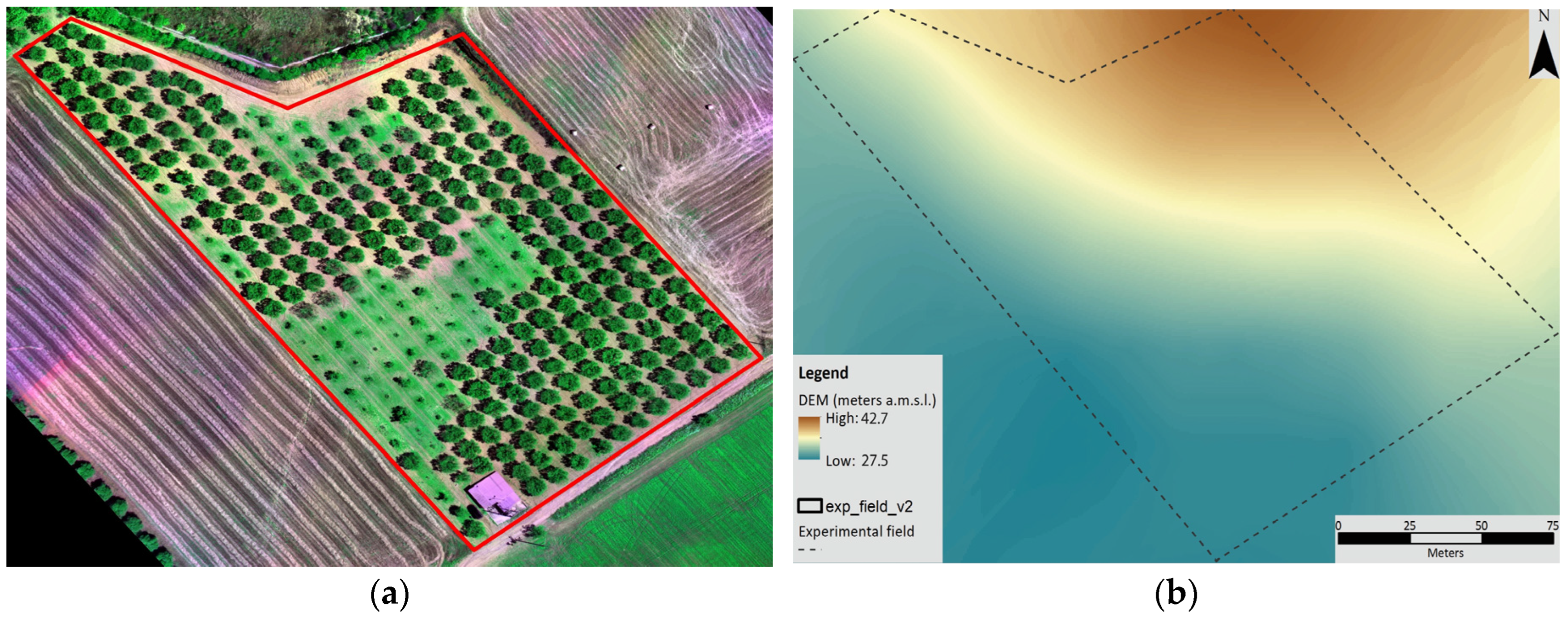
The experimental site was located in Halkidiki (Figure 1), a region in Northern Greece that is characterized by its robust agricultural industry.

A significant portion of the agricultural land in this area is dedicated to the production of olive trees. The production of extra virgin olive oil and table olives in the region is facilitated by many native varieties such as ‘Halkidikis’, ‘Amfissis’, ‘Kalamon’, ‘Galano’, ‘Metagitsi’, and ‘Agioritiki’. The ‘Halkidikis’ cultivar is highly regarded and favoured in the region because of its exceptional quality. However, it is also very susceptible to several challenges, both biotic and abiotic, with water stress being an ongoing concern.

The predominant crops in the region primarily comprise cereal crops and olives. In addition, there are dispersed agroforestry systems that consist of olive trees cultivated alongside cereals and herbs, serving as cover crops. The density of these trees typically amounts to roughly 800 trees per hectare. The area exhibits a mean annual temperature of 16.5 °C and a mean annual precipitation of 598 mm. In order to optimise crop production, a significant proportion of farmers employ irrigation techniques, predominantly relying on privately-owned groundwater pumps. This practice results in an environment favourable to the expansion and propagation of soil-borne fungal infections, including Verticillium dahliae, as well as airborne pathogens such as Spilocaea oleaginea and Cercospora beticola. The disease caused by S. oleagina is commonly known as peacock’s eye on an international basis, and as cycloconium within the region in which it occurs. Similarly, C. beticola is responsible for inducing the condition referred to as olive leaf spot. 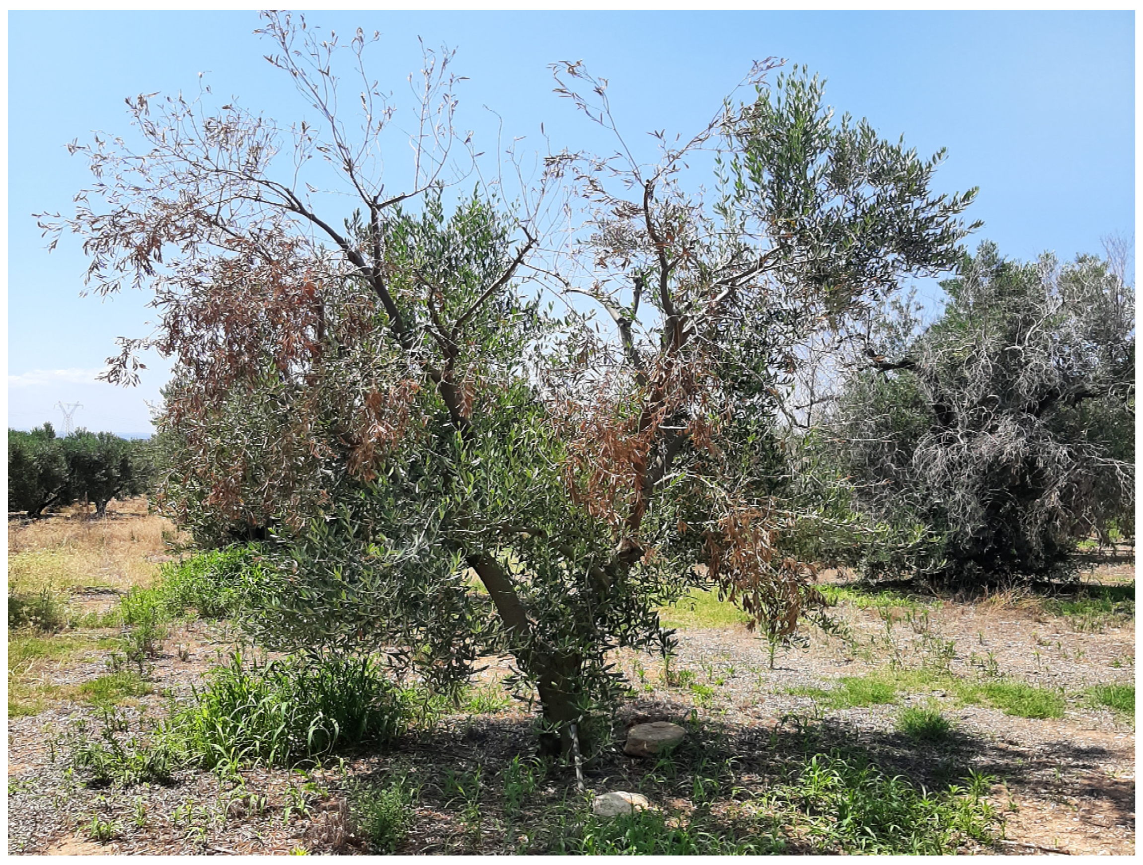The disease induced by V. dahliae is referred to as Verticillium wilt, characterized by symptoms that closely match those observed in olive trees under severe water stress (Figure 2), and is progressively affecting a growing number of agricultural areas annually.

The period between April and June in Northern Greece holds significance in the optimal growth of olive trees since it heavily affects their blooming stage. The producer of the experimental field (Figure 3) informed the research team about ongoing and accelerated infections observed each year caused by Verticillium wilt.

The infected trees were removed, and their remains were burned in an attempt to confine pathogen spread to neighbouring trees. Despite these efforts, some symptoms of initial infection could be observed in trees neighbouring infected trees.

2.2. Datasets and Pre-Processing

2.2.1. Data Collection

The sampling procedure for this experiment was conducted on 13 May 2021. Records of 76 trees in the olive field were collected by the researchers to assess initial symptoms of stress present in olive trees. The records were assessments for verticillium and other soil-borne pathogens, cycloconium, and other stressors. Each type of stressor assessment was accompanied by a numerical assessment ranging from 0 to 9, describing the infection levels present in each tree. After summing the three stressor assessments, the values for each sample concerning stress intensity ranged from 0 to 27.

A UAV platform with a rotary wing vehicle with 8 rotors was employed, with a Cubert S185 (CUBERT-GmbH, Germany) hyperspectral imager mounted on the platform. The imager obtained 138 available spectral band data with a spectral imaging interval of 4 nm, including a panchromatic band and 137 spectral bands in the range of 450–950 nm. The main parameters of the imager are listed in

Table 1. Cubert S185 spectral imager main parameters.

Parameters	Description
Wavelength range	450–950 nm
Sampling interval	4 nm
Full width at half maximum	532 nm@8 nm
	850 nm@25 nm
Bands	137
Focal length	16 nm
Horizontal field of view	22°
Digital resolution	12 bit
Detector specification	Area assay Si CCD
Weight	490 g
Power	DC 12 V, 15 W

.

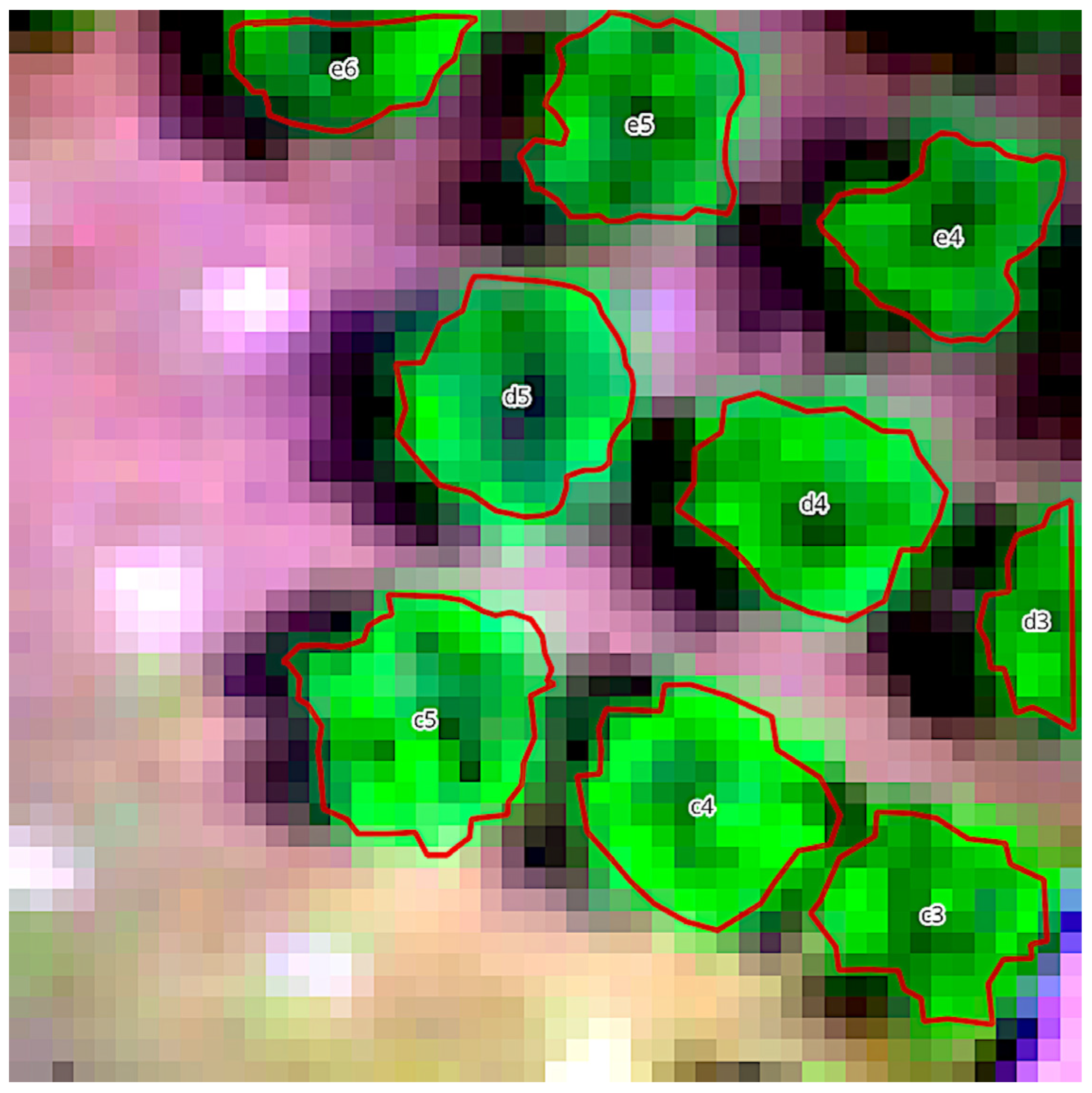
The hyperspectral data acquisition process involved both radiometric and spectral calibration of the hyperspectral imager. Radiometric calibration was carried out using standard white reference panels, to correct for sensor noise and ensure accurate radiance measurements. Spectral calibration was also performed, using known spectral light sources to ensure precise wavelength alignment and accuracy. These calibrations were conducted in controlled laboratory settings prior to data collection, and were supplemented with field calibrations to account for environmental variability. In total, 15 .tiff hyperspectral images were collected for this experiment, capturing a different amount of trees in each image depending on the density of each particular location in the field (Figure 4).

2.2.2. Pre-Processing

QGIS software (ver. 3.28.0) was used to load and extract the hyperspectral information in the form of Digital Numbers (DN) of each image and each band of the imager. This procedure involved digitizing the circumference of each tree/sample in the collected hyperspectral images, as seen in Figure 4. Then, the ‘zonal statistics multiband’ add-on for QGIS [31] was used to compute zonal statistics for each digitized tree/sample. The zonal statistics were associated with pixels enclosed by the digitized polygon shape of the tree vegetation.

The statistics computed for each band and each sample, regarding pixel values, were the count of pixels in the polygon; the sum; mean; median; standard deviation; minimum; maximum; range; minority; majority; and variance. This resulted in a matrix with 11 statistics for 137 bands, totalling an amount of 1507 independent variables for each sample. These will be called ‘features’ in the rest of the manuscript, based on the manner in which they were used by the classifiers.

Python 3 and Jupyter notebooks were used in the Visual Studio code IDE for additional data pre-processing. The zonal statistics and tree/sample records were loaded in a data frame using the Pandas python library.

A threshold of 10% was selected for attributing the ‘stressed’ or ‘healthy’ labels in each sample, meaning that samples that presented symptoms of damage or stress in over 10% of their vegetation were categorized as showing early signs of infection or abiotic stress and were classified as ‘stressed’.

The features were normalized in a range of −1 to 1, to remove the effect of varying numerical ranges in the dataset during the following steps of the modelling procedure.

To address the issue of class imbalance and, specifically, the number of positive instances in the minority class, the Synthetic Minority Over-Sampling Technique (SMOTE) was used [32]. SMOTE is an algorithm for addressing class imbalance in machine learning. It identifies the minority class, which was the ‘stressed’ class; selects instances; and generates synthetic samples by interpolating between them and, in this case, their 2 nearest neighbours. By adding these synthetic instances to the original data, SMOTE effectively balances class distributions, preventing bias toward the majority class and improving the model’s ability to learn from the minority class.

2.3. Feature Selection Methods and Modelling

Two feature selection and elimination methods were tested. The first was Recursive Feature Elimination (RFE), which is a feature selection technique used to systematically reduce the dimensionality of a dataset. RFE was used as follows: Initially, a machine learning model or classifier is trained using all available features. In our case this was tested with RF and XGB. Subsequently, the least significant features are identified and removed from the dataset. The model is then retrained with the reduced feature set. This process is iteratively repeated until a specified number of features remain. By selecting and retaining only the most informative features, RFE supports the enhancement of model interpretability, reduces overfitting, and potentially improves predictive accuracy. This is particularly important for the specified study, where redundant features or noise may be present.

The RFE method includes removing the x worst performing features during iterations for training the selected classifier, and has a step parameter to determine x. This is particularly useful for datasets such as this, where there is a high number of features, and training and evaluating models and features slows the process considerably. To address this, a step higher than 1 can be selected to remove more features during each iteration and lower the duration of the RFE process. This, however, may remove a feature that has a low—but not the worst—performance in an iteration, but may result in being one of the top performing features that will eventually remain in the pool of optimal features. During this experiment the step for worst performing feature removal was 1, to avoid losing valuable information. At the same time, not knowing beforehand the number of features that would be considered optimal for our case, an iteration was used to run RFE while selecting an increasing number of features to keep in, up to 10, and evaluating the changes in model performance for both classifiers.

The second method employed was Mutual Information (MI) feature selection, which is an approach used to assesses the degree of dependence between individual features and the target labels. MI quantifies the information shared between the features and the target labels, with higher values indicating stronger associations. In the context of feature selection, features with the highest MI scores are selected, while features with lower scores are discarded. This ensures that the spectral information most discriminative for identifying stressed labels is effectively utilized, enhancing the performance of the classification models employed using the features selected by MI for training and validation.

The machine learning algorithms employed and compared in this research were Random Forest (RF) and Extreme Gradient Boosting (XGB), without focusing on excessive hyperparameter optimization to assess classification performances, but rather on an out-of-the-box employment of the algorithms to assess the models’ performance based on the utilization of the two feature selection methods. RF [33] is an ensemble learning method that operates by constructing a multitude of decision trees during training. The output for classification tasks, such as detecting plant stress, is determined by the mode of the classes’ output by individual trees. While RF does not follow a single equation, its operation can be summarized as follows: For a set of training data X and labels Y, RF creates multiple decision trees. Each tree T_i gives a prediction Y_i for input X. The final prediction is the mode of these outputs. In this study, the input data for RF is comprised of spectral bands’ zonal statistics derived through hyperspectral images of olive trees, processed into a set of spectral features. The output is the classification of the incidence of stress in the trees.

XGB [34] is a gradient-boosting framework that builds an ensemble of decision trees in a sequential manner, where each tree attempts to correct the mistakes of its predecessor. This method is particularly effective for complex datasets, like hyperspectral imagery. The objective function in XGBoost combines a loss function L(Θ) and a regularization term Ω(Θ). The model is built by adding trees that minimize this function, with predictions y_i updated in each round n as:

$${\widehat{y}}_i^n={\widehat{y}}_i^{(n-1)}+\eta \times f_n\left(x_i\right)$$

(1)

where f_n is the decision tree added at the nth round, and η is the learning rate.

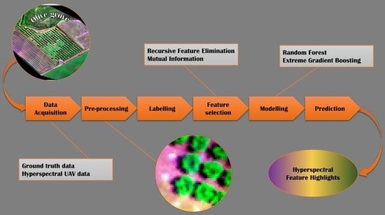
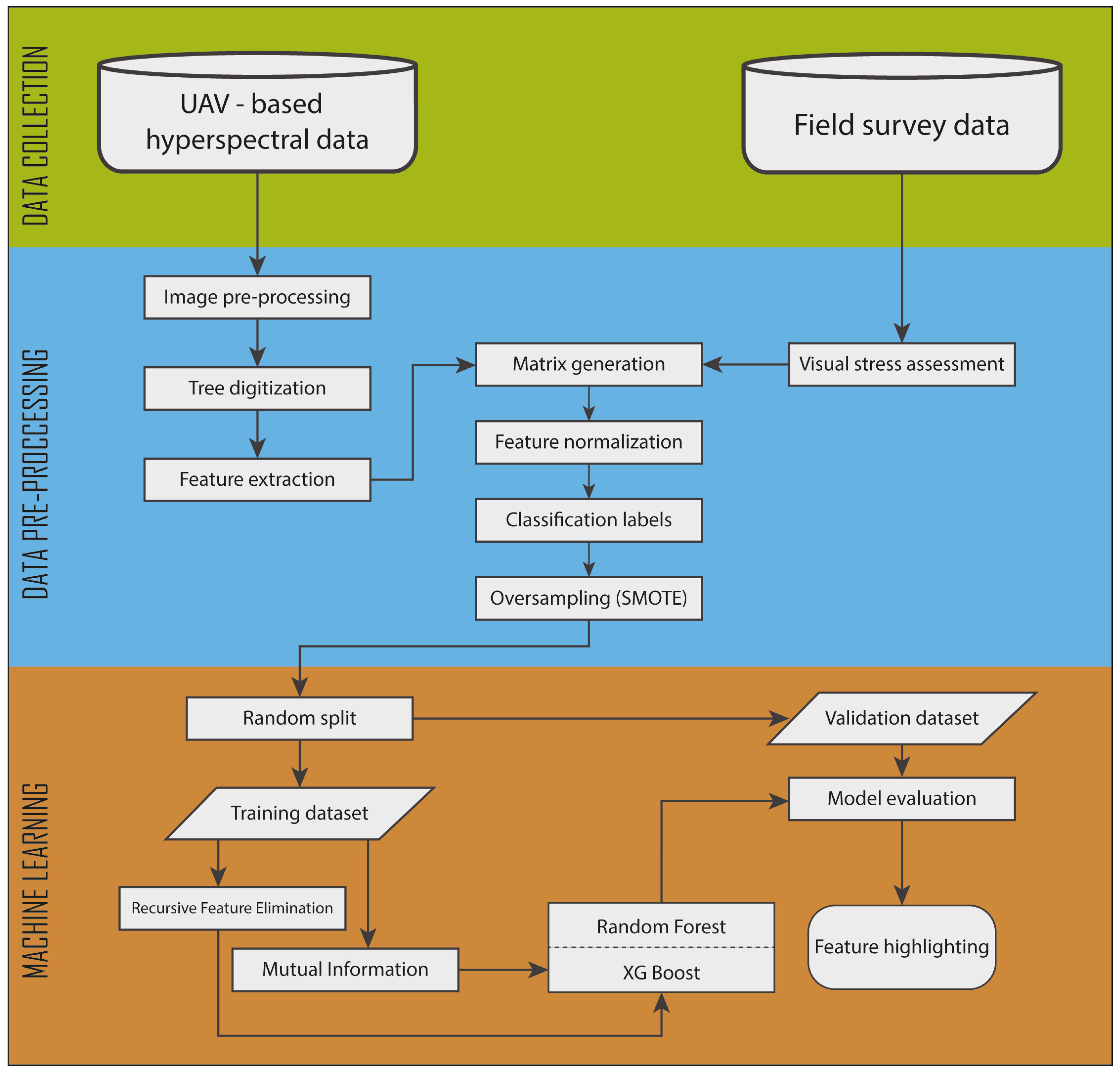
XGB was selected as it uses many parameters to allow the algorithm to avoid overfitting and, although more complicated to set up compared to RF, it usually provides better performance and robustness. The flowchart in Figure 5 describes the pipeline process followed in this study.

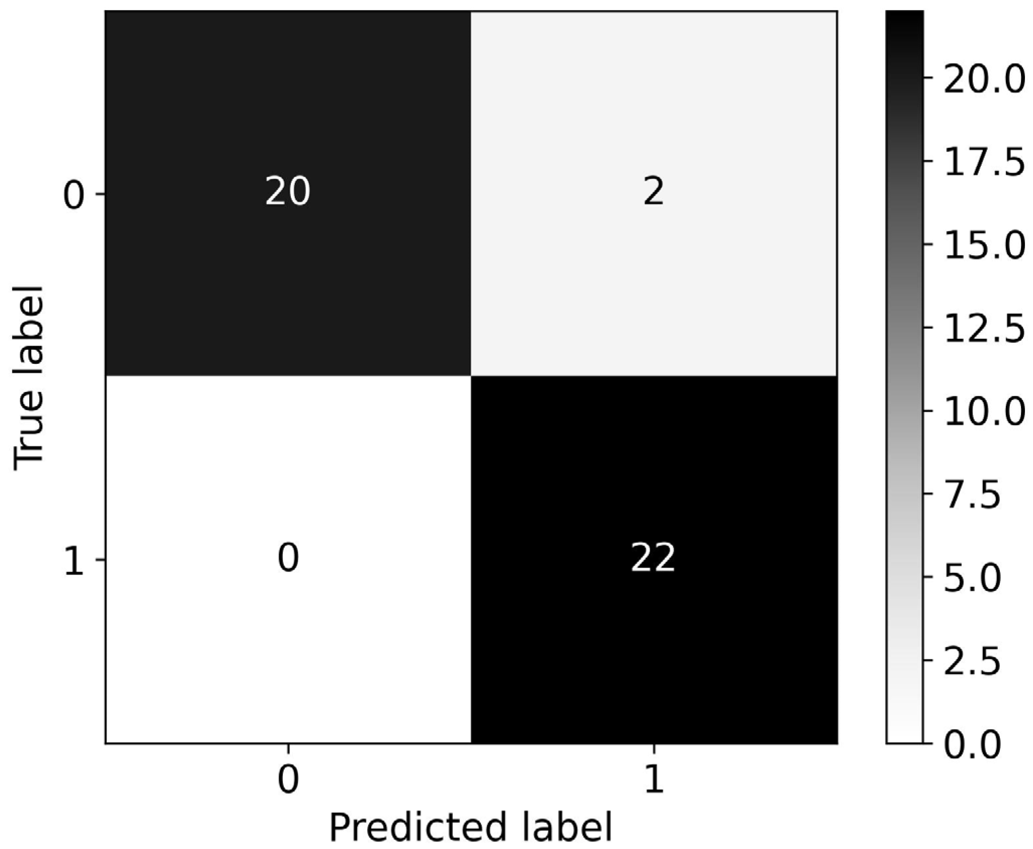
The generated models were evaluated using the area under the receiver operating characteristic curve (roc-auc) metric, which provides a summarized assessment of the models’ discriminatory power by measuring the trade-off between the true positive rate, or sensitivity, and the false positive rate, or 1-specificity. The values for the roc-auc performance metric range between 0.5, for models with the lowest performance that provide random classifications, and 1, for models with excellent performance.

3. Results

The results displayed that initial symptoms of diseases can be detected through the use of hyperspectral data with an accuracy of 100% using a RF and an XGB classifier, alongside feature selection methods to reduce the dimensions of the available dataset.

The RF and XGB classifiers were trained with the initial dataset of 1507 features, to compare changes in performance with the use of the fewer features that were obtained after applying the two feature selection methods. RF produced a model with a roc-auc of 0.977, slightly outperforming XGB, which produced a model with 0.955 roc-auc. The associated confusion matrices for the RF and XGB models can be seen in Figure 6 and Figure 7, respectively.

Table 2. Synopsis of results for all tested methods.

Classifier Type	Feature Selection Methods	Number of Features	Roc-Auc Score
RF	No feature selection	1507	0.977
XGB	No feature selection	1507	0.955
RF	RFE	5	1.00
XGB	RFE	2	1.00
RF	MI	3	1.00
XGB	MI	3	1.00

, below, provides an overview of the combination of the tested models and feature selection methods, together with the resulting roc-auc performances and optimal number of features. A more detailed description is presented in the following sub-sections.

3.1. Recursive Feature Elimination Results

3.1.1. Random Forest

Based on Figure 8, for RF classifiers the performance with only one feature was 0.864, and when using two features a performance of 0.977 was achieved, which is the same as when using all 1507 features. Performance remained the same when increasing the features from two to four, and achieved the highest performance of 1.00 when using the five best contributing features. The wavelengths and statistics associated with the features used for creating the model with the best performance were 650 nm (majority), 669 nm (majority), 687 nm (sum), 691 nm (sum), and 695 nm (sum). Adding more features than five drops the performance to 0.977, and it is safe to assume that it remains so for all following additions of features, as it is the same performance observed when training the classifier with all available features.

3.1.2. XG Boost

XG Boost classifiers achieved a high performance even when using one feature, having a roc-auc of 0.909. The highest performance is achieved when training an XG Boost classifier with the two optimal features, having a score of 1.00. The wavelengths and statistics associated with the optimal features are 654 nm (majority) and 680 nm (sum). When using additional features for training classifiers, model performance drops to 0.955, which also matches the performance achieved when using all 1507 available features (Figure 9).

3.1.3. Mutual Information Results

MI was used to acquire the optimal ten features for predicting our target classes. As MI does not select features based on a classifier selected by the user as opposed to RFE, the derived features are the same in both cases. The target objective here was to identify how many features of those selected by MI are required to achieve the highest performance for both classifiers.

For RF it can be observed in Figure 10 that three features are enough to produce a model with a score of 1.00, although using just one or two features still results in models with high performance, having roc-auc scores of 0.909 and 0.977, respectively, the latter also being the score for the RF classifier trained with the initial dataset of 1507 features. The wavelengths and statistics associated with the three optimal features are 552 nm (majority), 760 nm (majority) and 935 nm (range). While adding a fourth feature still results in an exceptional model with a score of 1.00, it is unnecessary, and continuing to add more features above four for classifier training drops performance to scores of 0.977 and lower, which, while still being high, do not provide better-performing models.

Figure 11 displays the performance of XGB classifiers for an increasing number of optimal features as selected by MI. Here, the pattern for the obtained scores is identical to the scores also obtained by RF up to using four optimal features. After that, XGB classifiers also provided high scores of 1.00 for additional features up to seven, and then dropped from eight features onward to a—still high—score of 0.932. Following the same logic as before, it was deemed that using additional features beyond the first three, while still having optimal scores, does not provide any benefit to the model. Because both models require three optimal features, as highlighted by MI, to produce the model with the highest quality, the wavelengths associated with the optimal features are the same for both cases, being 552 nm (majority), 760 nm (majority), and 935 nm (range).

4. Discussion

4.1. Evaluation of Classifier Performance

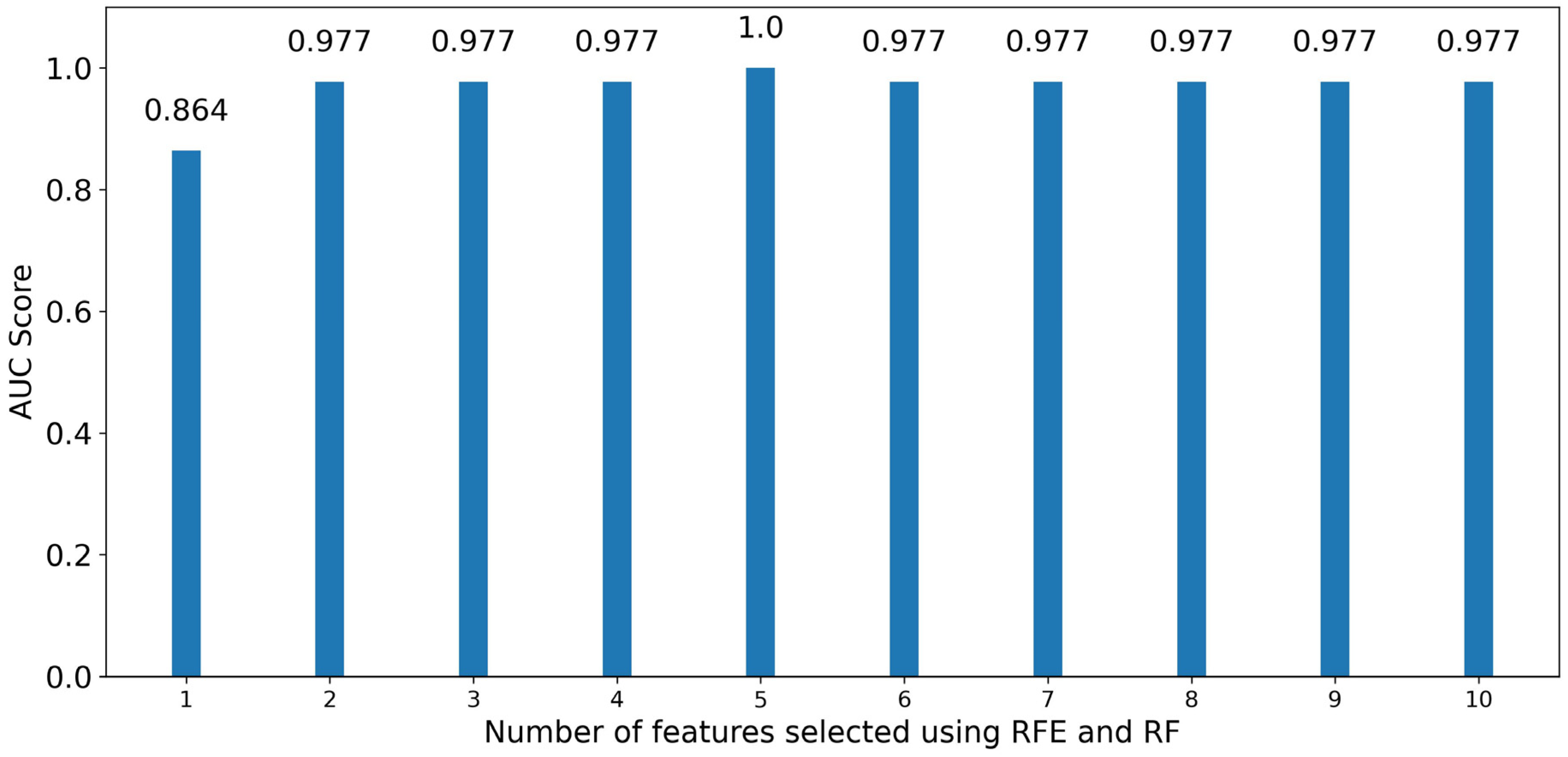
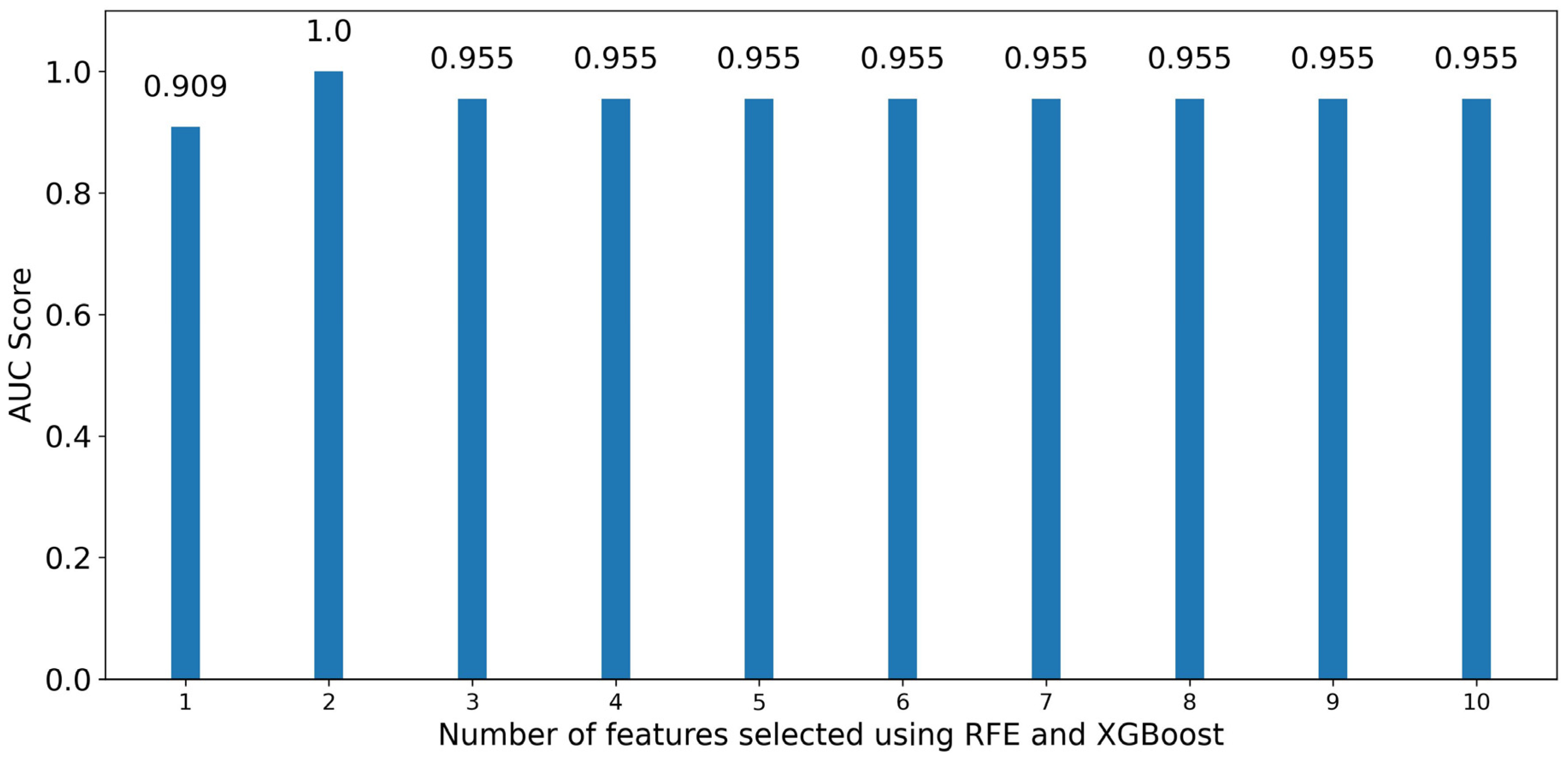
The findings from this study provide a comprehensive evaluation of the detection of stress in olive trees using hyperspectral data analysed with RF and XGB classifiers. Both the RF and XGB algorithms performed exceptionally well in detecting stress, with RF having a slight edge with a roc-auc of 0.977 compared to the 0.955 of XGB when trained with the full set of features, as was the case in a study by Adam et al. where they used a Random Forest algorithm and hyperspectral data to detect early stages of leaf spot disease in maize [35]. The performance of these models suggests that machine learning approaches, specifically ensemble methods like RF and XGB, can effectively distinguish stress signatures in hyperspectral images of olive trees. This has also been demonstrated in a case of detecting Xyllela fastidiosa in trees using a machine learning framework utilizing RF, XGB, and Gradient boosting [36].

4.2. Feature Selection Insights

A notable result from this study was the impact of feature selection on the classifier performance. Both algorithms achieved optimal performance with a minimal subset of features. For RF, the performance when using RFE peaked with five features, and for XGB, a perfect roc-auc score was obtained with two optimal features. This indicates that the dimensionality of the data can be significantly reduced without loss of performance, and highlights that XGB was more efficient than RF when reducing dimensionality in the dataset using RFE. This is also a critical insight for practical applications as it can reduce computational cost and complexity, as shown in [37] where dimensionality reduction was applied to hyperspectral data collected from a UAV-mounted camera, resulting in better-performing algorithms using fewer spectral features for training.

The stability of performance with an increasing number of features until a certain threshold supports the idea that beyond a critical point, additional features may introduce noise rather than informative variance. This is evident as the performance for RF does not improve past five features, and for XGB past two features, which emphasizes the importance of an appropriate feature selection method in hyperspectral data analysis.

The application of MI as a feature selection method also resulted in equal, optimal performance for both classifiers when the top three features were used. The consistent achievement of perfect scores with a model using just three features derived from MI is particularly noteworthy, implying that MI effectively captures the most relevant information for stress detection in olive trees, and its classifier-agnostic nature makes the selected features robust across different machine learning methods.

The fact that both RF and XGB classifiers did not benefit from additional features beyond the optimal number selected by MI further reinforces the idea that a small number of highly informative features can be sufficient for accurate classification, as also suggested by [38]. This finding is crucial for hyperspectral data processing where hundreds of features are often available, and selecting the most informative ones is challenging.

4.3. Correlation between Highlighted Wavelengths and Olive Tree Diseases

The study’s results have several implications for the analysis of hyperspectral data in agriculture. The high performance achieved with a limited number of features implies that there could be specific wavelengths that are particularly informative of stress in olive trees. This could lead to the development of simplified and more cost-effective sensors that only capture key wavelengths.

Additionally, the observed high roc-auc scores suggest that the selected wavelengths and statistical measures (majority, sum, and range) at those wavelengths are likely to be closely associated with the physiological changes in stressed olive trees.

Olive tree diseases such as Verticillium wilt, peacock’s eye, and olive leaf spot can manifest in ways that potentially alter the reflectance properties captured in the highlighted wavelengths. These diseases often lead to physiological changes such as chlorosis, defoliation, and disruption of water transport, which can be detected through hyperspectral imaging.

The wavelengths identified in the study as optimal for stress detection in olive trees—650 nm, 669 nm, 687 nm, 691 nm, 695 nm, 552 nm, 760 nm, and 935 nm—span across the visible to near-infrared (NIR) spectrum. In the context of plant physiology, wavelengths in the visible spectrum, particularly around 650–680 nm, are known to correspond to the absorption of chlorophyll, which is a critical pigment involved in photosynthesis. The detection of stress at these wavelengths could suggest alterations in chlorophyll content, which is often a response to stress factors such as disease, nutrient deficiencies, or water stress.

For instance, Verticillium wilt may lead to a decline in chlorophyll content as it interferes with water uptake and causes wilting and yellowing of leaves. The wavelengths in the visible spectrum (650–680 nm), which are sensitive to chlorophyll content as also mentioned in [39], would likely reflect these changes. A decline in chlorophyll may result in higher reflectance in these bands, which could be what the classifiers are picking up as indicators of stress.

Similarly, peacock’s eye and olive leaf spot are fungal diseases that create lesions on leaves, potentially increasing reflectance in the green spectrum (around 552 nm) due to leaf discoloration and structure alteration. These diseases could also impact the NIR reflectance (760 nm and 935 nm) by affecting the internal leaf structure and water content, both of which are critical to the spectral signature in these regions.

Furthermore, the 695 nm wavelength falls within the red edge region, which is sensitive to chlorophyll concentration and can indicate changes in leaf cellular structure often associated with stress responses [40]. The performance of classifiers using features at these wavelengths confirms their relevance in detecting physiological changes in the trees.

In the NIR spectrum, the wavelengths of 760 nm and 935 nm are associated with water content in the plant tissues and water stress, which is also related to Verticillium wilt. The 760 nm wavelength is close to the water absorption feature, which can indicate changes in plant water status—a common stress response in plants [41]. The 935 nm wavelength is also associated with water, but is more related to water vapor in the atmosphere, which may influence the detection of stress through changes in the transpiration rates.

Interestingly, there is a commonality in the key wavelengths identified by both RF and XGB classifiers after feature selection, particularly those identified by MI—552 nm, 760 nm, and 935 nm. The 552 nm wavelength, located in the green region of the spectrum, is known to reflect plant vigour and health, with stressed plants typically reflecting more green light due to chlorophyll breakdown or leaf thinning.

The recurrence of certain wavelengths among the tested methods suggests that there are specific spectral features strongly correlated with stress in olive trees. The consistency of these wavelengths across different feature selection methods and classifiers underscores their potential as reliable indicators of stress.

4.4. Novelty and Uncertainties

While the use of RF and XGB algorithms in hyperspectral data analysis has been established, their application to olive trees, especially for stress detection, is relatively unexplored. This study tailors these advanced machine learning techniques specifically to the nuances of olive tree physiology and stress indicators. The current research goes beyond the mere application of RF and XGB classifiers, and provides detailed analysis on the impact of feature selection, particularly demonstrating how a minimal subset of hyperspectral features can achieve optimal performance. This insight is crucial for practical applications, as it suggests that efficient and cost-effective monitoring of crop health is feasible with reduced computational complexity. The specific wavelengths that are most informative regarding stress detection in olive trees are also analysed in depth, providing not only an application of a machine learning model, but a detailed assessment of the physiological implications of spectral signatures’ correlations with various olive tree stressors. The consistency in the key wavelengths, identified by both RF and XGB classifiers with both feature selection methods, provides a robust validation of these spectral features as reliable indicators of stress. This cross-methodological agreement strengthens the case for these specific wavelengths being critical in stress detection.

This study on hyperspectral data for disease detection in olive groves, though insightful, is limited by dataset specificity and disease range. Although the findings are significant, limitations exist in the form of dataset specificity and disease range. Additionally, while successfully utilising feature selection methods like RFE and MI, the efficacy of these methods in broader applications remains to be tested. There is a possibility that the features identified as most informative in this study may not be as effective in different scenarios or with different diseases. Also, olive trees are susceptible to a wide range of biotic and abiotic stresses, and the ability of the algorithms to detect other types of stress remains untested. Expanding the scope of the research to include a wider array of olive tree diseases and stress factors would provide a more comprehensive understanding of the algorithms’ capabilities.

4.5. Practical Applications

Utilizing the findings of this research creates potential for building simplified hyperspectral cameras focusing on the most informative wavelengths for olive stress detection. Such specialized equipment could significantly streamline field surveys and reduce operational costs. Furthermore, embedding the highlighted, optimized machine learning models into real-time monitoring systems could revolutionise precision agriculture, facilitating early detection and more effective management of diseases in olive trees.

5. Conclusions

This research aimed to assess the effectiveness of machine learning algorithms, specifically Random Forest and XGBoost, combined with feature selection techniques, in detecting stress in olive trees through hyperspectral imaging. The study’s findings provide substantial evidence that machine learning classifiers can discern stress signatures with high accuracy when trained on hyperspectral data.

The RF classifier demonstrated a slightly superior performance, closely followed by the XGB, indicating that both classifiers are highly competent in identifying stress conditions. Feature selection emerged as a critical step in the classification process, with Recursive Feature Elimination and Mutual Information being instrumental in enhancing the classifiers’ performance by identifying the most informative features, emphasizing the power of feature reduction to not only maintain, but also improve classification accuracy.

A set of wavelengths that were particularly predictive of stress was highlighted, suggesting that targeted hyperspectral imaging could become a more cost-effective approach to stress detection in precision agriculture.

Following studies should aim to validate these findings across diverse environmental conditions and olive varieties; explore additional machine learning techniques; and aim to integrate these into practical monitoring systems for comprehensive disease management. By simplifying data collection and processing, more efficient and timely decision making is enabled in plant protection measures, potentially reducing losses due to stress and diseases.