Abstract
The latest development of multi-robot collaborative systems has put forward higher requirements for multi-sensor fusion localization. Current position methods mainly focus on the fusion of the carrier’s own sensor information, and how to fully utilize the information of multiple robots to achieve high-precision positioning is a major challenge. However, due to the comprehensive impact of factors such as poor performance, variety, complex calculations, and accumulation of environmental errors used by commercial robots, the difficulty of high-precision collaborative positioning is further exacerbated. To address this challenge, we propose a low-cost and robust multi-sensor data fusion scheme for heterogeneous multi-robot collaborative navigation in indoor environments, which integrates data from inertial measurement units (IMUs), laser rangefinders, cameras, and so on, into heterogeneous multi-robot navigation. Based on Discrete Kalman Filter (DKF) and Extended Kalman Filter (EKF) principles, a three-step joint filtering model is used to improve the state estimation and the visual data are processed using the YOLO deep learning target detection algorithm before updating the integrated filter. The proposed integration is tested at multiple levels in an open indoor environment following various formation paths. The results show that the three-dimensional root mean square error (RMSE) of indoor cooperative localization is 11.3 mm, the maximum error is less than 21.4 mm, and the motion error in occluded environments is suppressed. The proposed fusion scheme is able to satisfy the localization accuracy requirements for efficient and coordinated motion of autonomous mobile robots.
1. Introduction
Multi-robot collaborative positioning technology has found extensive applications in defense and civil fields—including robot formation combat, unmanned driving, robot team field exploration, unmanned disaster rescue, and unmanned carrier cooperative handling—owing to the advancements in artificial intelligence, computer technology, and automation. The multi-robot system is more than just a combination of robots; it involves collaboration and cooperation. Each robot is equipped with different sensors to fuse information based on task requirements. The robots within the group maintain spatial relationships and achieve collaborative positioning through complex communication and information exchange processes. This enables support for formation patrol, emergency risk avoidance, sudden stop, and obstacle avoidance autonomously. Multi-robot cooperative positioning technology outperforms traditional single-robot positioning technology in terms of enabling faster global awareness and planning, thus enhancing the robustness and autonomous positioning capability of multi-robot systems through capability complementarity and redundancy increase. Additionally, the use of small robots with a single function facilitates fault detection and functional upgrades.
Positioning in robot navigation relies on sensors to perceive the surrounding environment, serving as the foundation and prerequisite for task execution. Common indoor robot sensors include inertial measurement units (IMU), odometers, vision sensors, laser range finders, and sonar detectors. Each sensor has its own advantages and limitations. Sensors that operate without relying on external signals offer fast sampling speed but suffer from significant cumulative error. Laser rangefinders exhibit high accuracy but can only determine object distances directly. Vision sensors excel in perceiving the environment and capturing rich environmental information. However, vision detection and localization algorithms necessitate high system computational performance, are influenced by ambient light and target characteristics [], and do not provide global positioning information for the robot. The fusion of the advantageous performance of each sensor is a promising research area aiming to reduce costs, enhance system robustness and flexibility, and enable seamless collaborative localization in multi-robot systems through the fusion of multiple information sources.
Multi-sensor fusion is a well-established algorithm in the field of robotics and control [,,]. It aims to integrate multiple sensors to enhance system performance and achieve precise positioning. Researchers worldwide have extensively investigated the robot localization problem by leveraging sensor information fusion. For example, Yan Lu and Joseph Lee et al. [] fused laser range information and sensor data from monocular vision to propose a fusion scheme for acquiring position information in GPS-denied environments. Howard and Gaurav S. fused mutual observation data from two robots [] and presented a method to localize members of a mobile robot team using the robots themselves as landmarks. Other researchers have employed various fusion algorithms, such as the extended Kalman filter method [,], which assumes a Gaussian distribution for systematic error and effectively addresses the prediction problem of nonlinear systems. Anastasios used an extended Kalman filter (EKF)-based algorithm for real-time vision-aided inertial navigation, which improved the fault tolerance performance of the measurement data []. There is also the use of great likelihood estimators to derive relative positions between robots [,], or real-time position estimation of robots using particle filtering [,,]. I.M. Rekleitis estimated a larger group of robots that can mutually determine one another’s position (in 2D or 3D) and uncertainty using a sample-based (particle filter) model of uncertainty in a specific scenario []. The application of co-localization results in multi-robot systems is also becoming a key issue of current interest. Boda Ning et al. were concerned with the collective behavior of robots beyond the nearest neighbor rule []. Brian Shucker proposed a control and communication scheme for multi-robot systems in long-distance situations with his team [].
The limitations of the existing multi-source co-location algorithms include a lack of real-time comprehensive state estimation from the sensors of different types of robots and the consideration of calculation burden, cost, and rigorous mathematical models. Most of the above research belongs to the primary stage; some have provided integration schemes for single-robot application scenarios. Furthermore, some research has the potential to involve multi-robot positioning and dynamic performance estimation realized by positioning each robot independently, but the actual systems are limited by high computation and maintenance costs. In addition, the state estimation performance degradation is more serious, partly caused by multistage errors in practical applications and the limitations of the current algorithm architecture.
As far as we know, there is a lack of research providing insight into the fusion of the laser rangefinder, camera, and other sensor data in heterogeneous robotic systems with varying levels of complexity and sensor configurations. This work makes three primary contributions. First, the co-position process gathers observations from both the robot itself and other robots, providing increased flexibility and robustness in sensor information fusion. Second, by leveraging the advantageous performance of diverse sensors, a variety of observation and communication tasks can be dynamically assigned to different types of robots, thereby improving overall task fulfillment and the system’s anti-interference capabilities. Third, the system can utilize small robots with simple structures and single functions, simplifying upgrades and maintenance compared to complex, independent robot systems.
The remainder of the paper is organized as follows. In Section 2, we present a method for a multi-sensor data fusion co-position scheme applicable to heterogeneous multi-robot systems and common navigation modes. Section 3 analyzes practical errors and suggests improvements. Section 4 showcases our experimental results, and Section 5 provides the conclusions.
2. Methods
2.1. Integration Architecture
Considering the flexibility, practicality, and scalability of the multi-robot system, the navigation mode chosen is a common Leader–Follower robot swarm. The main structure of the proposed integration is presented in Figure 1 and consists of three steps.
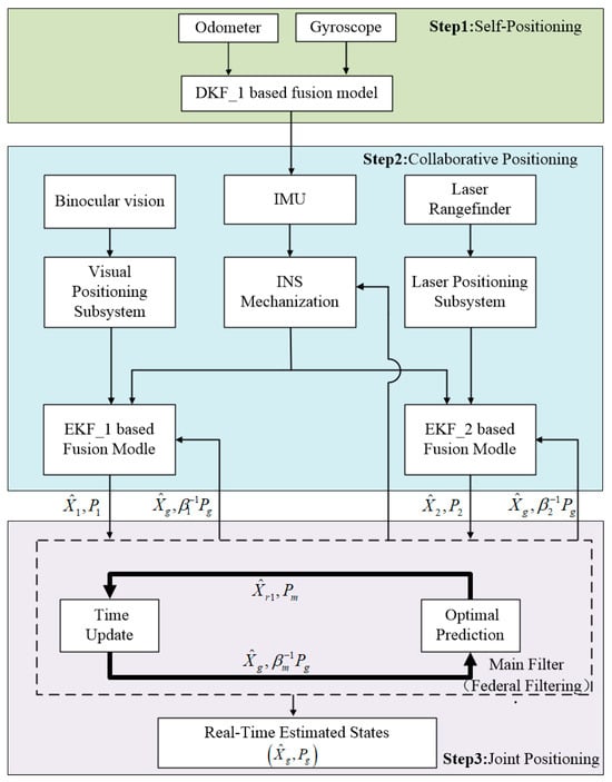
Figure 1.
Proposed joint filtering integration scheme.
The integration involves three sub-filters and one main filter. The first discrete Kalman filter, DKF_1, fuses the odometer and gyroscope information within the robot to determine the inertial system’s state equation. The extended Kalman filters, EKF_1 and EKF_2, estimate the target localization information using the vision sensor and laser rangefinder, respectively, with the inertial guidance system as a reference. The vision localization subsystem employs the improved YOLO deep-learning-based target detection algorithm and camera calibration algorithm to obtain target localization information. This information is then used as the observation input to estimate the target localization using the extended Kalman filter. Similarly, the laser ranging subsystem utilizes the angle between the target’s horizontal projection and the optical axis of the camera, obtained from the vision sensor, to obtain positioning information. This positioning information is used as the observation input to estimate the positioning state of the laser rangefinder using the extended Kalman filter. The main filter calculates the information allocation factor for each sub-filter and combines the estimated results using the extended Kalman filter, yielding accurate target localization.
2.2. Coordinate Frames Definition and Transformation
2.2.1. Definition of Global and Local Coordinate Frames
The positioning solutions provided by different sensors are expressed in different navigation systems and then integrated into a unified navigation frame for data fusion. In this paper, we mainly use the definition and transformation of global and local coordinate systems to describe the positioning of the surrounding environment, targets, and obstacles, and the corresponding coordinate systems are shown in Figure 2.
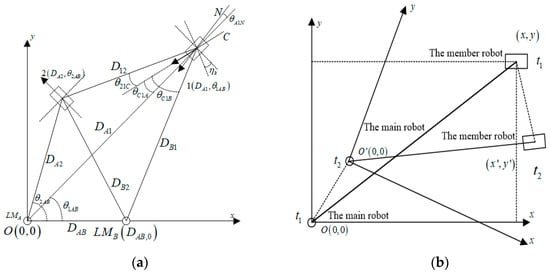
Figure 2.
Coordinate system framework for multi-robot systems: (a) global coordinate frame; (b) local coordinate frame.
The elements in the global coordinate frames are described as follows, where 1 and 2 represent the main robot and member robots, respectively. LMA and LMB are artificial road signs. N indicates the main robot heading, and DAB is the camera optical axis centerline direction of the main robot. Hk is the angle between the main robot heading N and the camera’s optical axis centerline direction. The robot-equipped sensors provide the following data: D12, DA1, DB1, θ21C, θC1A, and θC1B. D12, DA1, and DB1 can be obtained from the laser range scanner, while θ21C, θC1A, and θC1B can be read by the vision sensors. DAB and ηK represent known observation data. Based on the geometric relationships before each robot and the road signs, the positions of the member robots in the global coordinate system can be solved for and expressed in polar coordinates as
Similarly, the position of the master robot in the global coordinate system can be expressed in polar coordinate form as
The heading angle of the main robot at this point can be calculated as follows:
The local coordinate frame is employed to describe the relative positions of individual robots in a multi-robot queue, including the updated relationships during their travel. In this coordinate system, the current position of the main robot serves as the origin, and the current heading represents the positive x-axis. At time t1 in the figure, the position of the member robot in the x o y coordinate system is (x, y). The heading and position of the main robot change as it moves. At time t2, the coordinate system is updated to xo′y, and the position of the member robot is updated to (x′, y′). The time interval (t2 − t1) is defined as the coordinate system update step, during which the x o y coordinate system is utilized for both the main robot and the member robots.
2.2.2. Transformation of Visual Coordinate Frames
The purpose of using binocular vision [,] is to obtain the distance D between the target position and the camera by imaging the target in the vision sensor, and the angle θk between the horizontal 2D spatial projection of the target in 3D space and the centerline of the camera’s optical axis. In the camera point model, the point [x, y, z, l]T in 3D space is converted into the 2D spatial projection coordinates [u, v, l]T, which can be described by the following equation:
where fcx and fcy are the components of the camera focal length in the x and y direction respectively, and (cx, cy)T are the coordinates of the main point of the image. Due to daylight refraction, the imaging lens of the camera produces a certain radial deformation, which eventually affects the imaging of the target in the camera. Considering the effect of the mirror deformation factor, the projection coordinates of the point in 3D space in 2D space can be rewritten as
where k1, k2, and k3 are the refraction coefficients of light, r2 = (x/z)2 + (y/z)2. The parameters fcx, fcy, cx, cy, k1, k2, and k3 can be obtained by the camera calibration algorithm. After removing the radial deformation, the coordinates matrix of the target in the imaging plane are
The binocular vision imaging model is shown in Figure 3; vou and v’ou are the image imaging plane, z and z′ are the central optical axis of the camera, p(up, vp) and p′(up′, vp′) are the target O in the two planes of the imaging point.
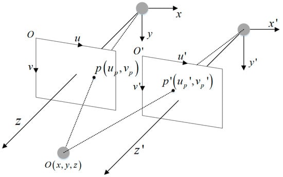
Figure 3.
Binocular vision imaging model.
Then, the angle η between the target O and the two camera’s center optical axes in the horizontal plane can be expressed as
where W is the actual physical width of the imaged image and 2α is the horizontal tensor angle of the camera.
2.3. Model Design
Referring to the joint filtering scheme in Figure 1, the model is designed using Leader–Follower as the navigation mode. Two types of robots in the swarm are equipped with different sensors. The main robot is equipped with internal sensors (odometer and gyroscope) as well as external sensors (laser range scanner and binocular vision system), and the member robots are only equipped with odometers, gyroscopes, and sonar arrays to reduce the cost. During the formation march, each robot performs self-localization using its internal sensor data. Simultaneously, the main robot utilizes vision and laser devices to observe the positions of the current member robots. However, due to significant cumulative errors in the internal sensors and observation errors caused by time delay and drift in the external sensors, the acquired positioning data deviate considerably from the actual positions.
2.3.1. Odometer and Gyroscope Integration (Step 1—Self Positioning)
Deducing the robot’s position and heading accuracy solely from the odometer data leads to relative cumulative errors. To enhance the accuracy, it is necessary to fuse these data with the gyroscope data. Given the linear system characteristics, this paper employs a discrete Kalman filter to fuse the data from both sources. Let X = [vL, vR, wg]T represent the state variables. The state equation of the system can then be expressed as
where Ak+1 is the state transfer matrix from k to k + 1 moments and Wk is the Gaussian white noise with covariance matrix Q. Referring to Deng et al.’s use of the sensor model in the outdoor mobile robot localization method [], the transfer matrix is
where β is the odometer correction factor determined down from the actual test data, and the system observation equation is
where the observations can be read from the odometer and gyroscope and the measurement matrix Hk is the unit matrix I.
2.3.2. Distributed Data Fusion of Visual Positioning Subsystem and Laser Observation Subsystem (Step 2—Collaborative Positioning)
- Inertial navigation system state derivation
Combined with the motion characteristics of the robot, we use the arc model to describe the motion of heading changes; the corresponding state derivation model is shown in Figure 4.
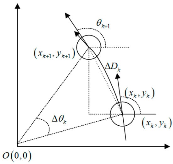
Figure 4.
State derivation model for INS.
The motion model of the inertial guidance system can be expressed as
where , is the input to the odometer model, Dk is the length of the arc, and θk is the change in steering angle; the values of the latter two are both obtained by fusing the odometer and gyroscope data. wk is the Gaussian white noise of the system with covariance matrix Q. Then, the gained Jacobi matrix A of the state equation can be derived from the motion model as
Assuming that its noise is Gaussian white noise, the covariance matrix Pk+1 of the model can be derived as
- 2.
- Visual target detection and localization
The visual localization process involves using a deep-learning-based convolutional neural network algorithm for target detection. This algorithm detects the visual targets and extracts their center coordinates. The subsequent steps include camera calibration to establish the mapping relationship between the camera coordinate system and the world coordinate system, and correcting lens deformation errors. Finally, the algorithm calculates the distance from the center point to the camera’s optical axis in the horizontal direction and the angle of deviation. This process enables accurate target localization. The complete visual localization algorithm process is depicted in Figure 5.
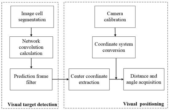
Figure 5.
Process of visual localization algorithm.
For robot target detection, we utilize an improved YOLO algorithm based on convolutional neural networks. This algorithm offers significant advantages in terms of precision, measurement speed, and accuracy [], making it suitable for multi-robot indoor mobile scenarios. Unlike traditional two-stage target detection algorithms that rely on candidate regions, the YOLO algorithm treats target detection as a single regression process. It employs a single convolutional neural network to predict the detection frame and its corresponding position confidence level. The main architecture of the algorithm, illustrated in Figure 6, comprises an input layer, a backbone network, and a neck and head network. The specific working process is as follows:
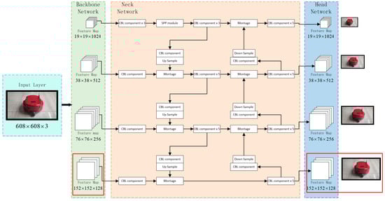
Figure 6.
YOLO algorithm network architecture.
The input layer completes the pre-processing of the input avatar, scales the input image to a fixed size, and completes the normalization operation. The network input size of the YOLO algorithm can be adjusted to meet a multiple of 32. The larger the input image size is, the more details are retained and the better the detection effect is, but at the same time, the image detection speed will be reduced. Combined with the image characteristics of the robot target, the network input size is set to 608 × 608 in this paper.
The backbone network, comprising five Cross Stage Partial (CSP) modules, is utilized to extract deep semantic information from the image. These modules propagate features to the CBM (Convolution operation + BN batch normalization + Mish activation function) convolution module while also sending them to the residual block. The results of these two convolutions are then combined using the concat splicing unit []. This design reduces computational effort, enables richer gradient combinations, and avoids the problem of gradient disappearance in excessively deep networks. Each CSPX module contains 5 + 2 × X convolutional layers, resulting in a total of 72 convolutional layers in the backbone network. When the input image size is 608 × 608, the operations performed by each CSP module, as well as the head CBM module, and the corresponding output results are depicted in Figure 4. The feature map changes from 608 to 304, 152, 76, 38, and 19, forming a three-layer feature map of sizes 76 × 76, 38 × 38, and 19 × 19, which constitute a feature pyramid.
The neck and head networks are utilized to extract fused features more effectively and accomplish multi-size target prediction, including the extraction of center coordinates. To enhance feature extraction and representation, the YOLO algorithm incorporates the PAN (Path Aggregation Network) structure after the Feature Pyramid Network (FPN) for feature fusion across different backbone layers. The neck network ultimately produces three standard-sized feature maps (76 × 76, 38 × 38, and 19 × 19) for multi-scale prediction by the head network. While this algorithm generally achieves good detection accuracy, there is a low probability of false detection in low-light environments or when encountering objects with similar shapes. To address this, we introduce an additional branch with a downsampling rate of 4 (resulting in a 152 × 152 feature map) to the original YOLO algorithm, which already includes downsampling rates of 32, 16, and 8 (corresponding to 19 × 19, 38 × 38, and 76 × 76 feature maps, respectively). This modification enables finer prediction results, enhances detection performance for smaller objects, improves the algorithm’s spatial differentiation capability, and effectively reduces the probability of false detection [].
Figure 7 showcases representative detection results achieved by the optimized YOLO target detection algorithm using the constructed dataset. The optimized algorithm demonstrates higher confidence in detecting target robots, road signs, and distinctive shape markers, meeting the accuracy requirements for visual localization.
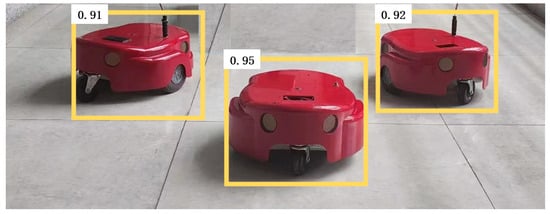
Figure 7.
Target detection.
If the distance between the two cameras of the binocular vision sensor is known to be D, and θ1, θ2 are the angles between the binocular camera line and the camera-to-target center line, respectively, then the distance from the midpoint of the binocular camera to the target center can be solved as follows:
If the main robot observes itself at moment k with coordinates (xk, yk), then its distance observation equation can be derived as
where vjg is Gaussian white noise, and its Jacobi measurement matrix can be deduced as
- 3.
- Laser observation and localization
If two colored cylinders are placed in the direction of the member robots’ heading, the distance difference between the two cylinders is obtained by the visual target detection method, and the robot heading can be calculated at this moment. The laser rangefinder positioning heading model is shown in Figure 8.
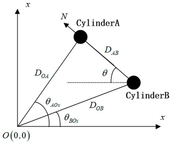
Figure 8.
Laser rangefinder positioning heading model.
The forward direction of the robot can be determined by using different colored cylinders. DAB is a known as a fixed distance; then, the robot heading can be deduced as
The heading observation equation of the laser rangefinder can be expressed as
where vjb is Gaussian white noise.
The real-time distance of the member robot relative to the main robot can be obtained according to the laser rangefinder model and Equation (8). Let the coordinates of the main robot itself at the time of observation be (xk, yk); then, the distance equation of the laser rangefinder is
From the above equation, its measurement matrix can be further deduced as
The total observation equation of the laser sub-filter can be obtained as
2.3.3. Joint Filtering Algorithm (Step 3—Joint Filtering)
Referring to the joint filtering model depicted in Figure 1, the process begins with the discrete Kalman filter performing data fusion of the odometer and gyroscope at the front end to estimate the real-time state of the inertial guidance system. Then, the visual sensor extracts the angle information of the target, which is then used to establish laser distance data, facilitating interaction and cooperation among the subsystems. Finally, the joint filtering model employs federated filtering to accomplish information fusion within the distributed sensor network. Specifically, the fusion involves using the extended Kalman filter to merge the state of the inertial guidance system, serving as the reference state, with the visual positioning and laser positioning subsystems. The estimation results from the two extended Kalman sub-filters are subsequently passed to the main filter, enabling optimal fusion of information and estimation of the system’s global state value X = [x, y, θ]T. The joint filtering algorithm comprises the following steps:
- Completing the solution of information allocation factors β1, β2. The information allocation factor βi satisfies the information conservation principle, which meansβm represents the information distribution coefficient of the main filter, while the value of β1, …, βn directly impact the performance of joint filtering. Typically, larger coefficient values are assigned to sensors with higher measurement accuracy. However, since the external sensor subsystem employed in this study may experience sudden measurement errors like drift, using a fixed coefficient value is not appropriate. Hence, we employ eigenvalue decomposition based on the true variance Pi to calculate the real-time value of βi. Pi can be decomposed by eigenvalues , where ; the value of βi can be deduced as
- Initialize the global state estimate value and the covariance matrix Pi0 and assign the information to each sub-filter and the main filter in proportion to the information factor βi:
- The time correction is applied simultaneously to each sub-filter and the main filter, and the common noise is allocated to each sub-filter based on the information factor βi:then, the filtering time is corrected towhere Γ is the system noise matrix and A is the state transfer matrix.
- Each sub-filter uses a local observation Zi for the observed data correction.where Hi is measurement matrix.
- Main filter completes information fusion [].where n is the amount of sub-filters.
3. Analysis and Correction of Practical Errors
The theoretical analysis presented above discusses the feasibility of cooperative localization and outlines its implementation process. However, in practical applications of multi-robot formation navigation, errors are inevitable. Therefore, it is crucial to analyze the causes of different types of errors and propose appropriate correction solutions.
3.1. Visual Target Detection Delay
The visual target detection algorithm studied in this paper consists of the following two main processes:
Firstly, the main robot observes manual road signs for self-positioning in the global coordinate system. The main robot uses target detection and extracts road signs from the environment to obtain the relative distance information between the camera and the road signs, which is fused with information from its INS to obtain accurate global positioning information. Secondly, the master robot observes the member robots and positions them for observation in a relative coordinate system. The main robot uses binocular vision sensors and laser rangefinders to locate the member robots and sends the position information to the member robots through the mesh network. The member robots use this information to fuse with their own inertial guidance systems to obtain accurate relative position information.
The visual target detection information is fused with the information from the inertial guidance system. However, this fusion process introduces errors due to the delay in target detection. The error can be managed through two approaches: first, by restoring the motion of the observed robot to its position prior to the time delay, and second, by reducing the target detection time to fall within the acceptable error range. Table 1 illustrates the time delay observed in each stage of the target detection process.

Table 1.
Time consumption of each stage of visual target detection.
The time required for the target detection process can be reduced to less than 15 ms by significantly reducing the image area to be inspected in indoor scenes. In the fusion strategy, no action is taken during the first imaging, and the data from the second imaging are used as observation data for the inertial guidance system. Assuming the robot moves at a speed of 600 mm/s, the observation error range caused by the target detection algorithm can be controlled to be below the millisecond level, thus meeting the localization accuracy requirements once again.
3.2. Network Communication Latency
The master robot transmits the observation and positioning information of the member robots to them through the mesh network. The member robots then integrate this information with their own inertial guidance systems to obtain precise real-time relative position information. In practical applications, there is a network time delay during communication. However, since the robots form a dynamic mobile network, the communication time delay is minimal, and the differences in time delay mainly depend on the real-time network conditions. To manage these errors, motion recovery is performed on the robots.
Figure 9 illustrates the initial assumption of the robot’s circular motion with a radius R around the origin O.
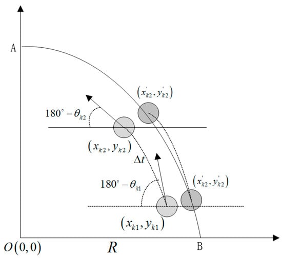
Figure 9.
Communication latency recovery model.
In the figure, (x, y) represents the actual position of the robot, while (x′, y′) denotes the estimated position observed when the member robot reaches the position (xk1, yk1). In the absence of network time delay Δt, the estimated position is corrected to (xk1′, yk1′) after filtering. However, due to the presence of time delay Δt, the actual position of the robot reaches (xk2, yk2) before the observations from the subsystem reach the member robots for fusion. If these data are fused with the inertial guidance system data, errors will occur. Assuming the sensors within the inertial guidance system have undergone internal fusion n times within Δt time, the sequence of state estimates is preserved {X1, X2, …, Xm}, where X = {x, y, θ} and m > n. After receiving the observation from the network, the member robot calculates the network time delay Δt, retrieves the state estimate from the inertial guidance system’s state estimation sequence at the corresponding time point for fusion filtering, and the filtered state estimation point should be (xk1′, yk1′). Then, a state sequence is established, representing the correlation chain of the robot’s internal sensor adjustment angle. By fitting a trajectory that progresses from the point (xk1′, yk1′), the corrected position (xk2′, yk2′) that the robot should adopt at that moment is obtained.
3.3. Observation Masking
Both visual imaging and laser ranging rely on line-of-sight observations. If the camera–target line is obstructed by other objects, the target cannot be detected and positioning information cannot be obtained. In multi-robot formation movement, the main robot and member robots may be occasionally obstructed by other robots or obstacles. Figure 10 illustrates a scenario where the member robots are obscured by each other. In the figure, R1 represents the main robot; R2 and R3 represent the member robots; and N1 and N2 indicate the headings of R1 and R2, respectively. When all three robots align in a straight line, as shown in the figure, R1 and R3 are obstructed by R2, rendering R3 unobservable by R1.
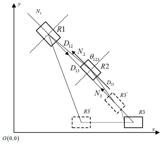
Figure 10.
Robotic observation masking model.
This problem can be addressed by considering two cases. The first case occurs when R3 moves to its next position R3′, implying that R2′s obstruction of R3 is temporary. In this situation, R2 only relies on its own inertial guidance system to track its motion trajectory during the period of obstruction. Once R2 passes the obscured area, it can then use observation information from the main robot to make corrections. The second case occurs when R3 maintains the same heading as R2 and the three robots move in a straight line for an extended period. In this scenario, R1 is unable to observe R3 for an extended duration; so, we utilize R3′s own sonar array positioning to make position corrections. The distance D12 between R1 and R2 in the figure can be measured because R2 is in the heading direction of R3, and its sonar array emits waves in this direction with a certain level of accuracy. Additionally, the small angle formed by the heading direction of R3, where R2 is located, can be determined through the geometric relationship between global positioning, allowing us to measure D23. Therefore, the distance between R3 and the main robot can be deduced as
3.4. Requirements of the Filtering Process for the Observed Values
The equation for the observation of the main robot to the member robots in relative coordinates is
The observation equation converted to relative orientation is
where θj is the current heading of the main robot, and vφ is the Gaussian white noise with zero mean and variance of δφ2, when
This implies that the Δx between the two robots is very small, and minor measurement errors can lead to significant deviations in the orientation observation, thereby causing challenges in filter convergence []. Therefore, when the relative orientation is near ±(π/2), the relative orientation observation does not provide useful localization information. Hence, prior to the filtering update, the observation is evaluated and selected based on the 3δφ law. If the difference between the observation and the expected value exceeds 3δφ, the observation is discarded. Subsequently, if the observation satisfies the condition , it is determined to fall within the range of ±(π/2) and cannot be used for the filtering update. However, the state update of the inertial guidance system is still employed.
4. Results and Discussion
4.1. Test Platform
To evaluate the performance of the multi-robot cooperative localization algorithm in an open indoor environment, we designed a multi-robot experimental platform consisting of a main robot and three smaller robots, as shown in Figure 11a.
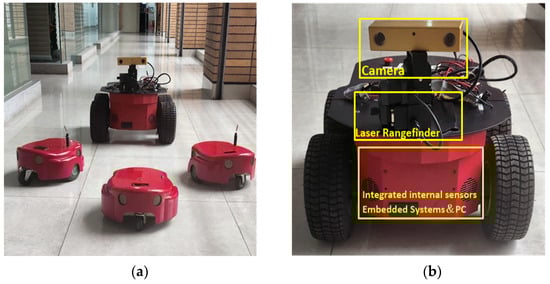
Figure 11.
Test platform and equipment. (a) Multi-robot system formation scenario. (b) Main robot and main sensors.
As shown in Figure 11b, the main robot is equipped with an onboard computer that possesses processing and computing capabilities. It can be connected to a WiFi device with a USB interface to facilitate communication among the multi-robot systems. The member robots are equipped with microcontrollers responsible for motion system state processing. In the actual experimental setup, the multi-robot platform utilizes a SICK laser range scanner for distance measurement, and member robots are equipped with sonar arrays as their distance sensors. The main robot is equipped with a rotating binocular vision sensor, enabling the target image to be positioned as close to the center of the field of view as possible, thus improving positioning accuracy. All experiments are conducted and performed on this platform, with different experimental scenarios varying in the combinations of robots and sensors. The configuration program of the multi-robot system’s experimental platform equipment is shown in Table 2.
Table 2.
Multi-robot experimental platform equipment configuration program.
4.2. Test Scenarios
Three field tests were designed and conducted to assess the performance of the proposed scheme and analyze error characteristics. Test Case 1 aims to evaluate the fusion of odometry and gyroscope information using discrete Kalman filtering. Test Cases 2 and 3 are implemented in a multi-robot system performing formation marching, as illustrated in Figure 12, where the black circle represents the main robot and the white circles represents the member robots.
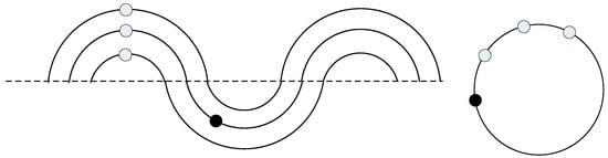
Figure 12.
Positioning experimental trajectory of Test Cases 2 (the left part) and 3 (the right part).
Test Case 2 examines the performance of the joint filtering localization algorithm during S-curve motion, where the master robot leads the member robots in formation. Test Case 3 investigates the actual localization error in the presence of observation occlusion when the multi-robot system moves in a circular trajectory. The deviation is calculated by comparing the actual robot motion trajectory with a specified high-precision reference trajectory.
All robots are equipped with WiFi communication devices that support IEEE802.11 series protocols, enabling the formation of a dynamic mesh network for data communication among them. The specific experimental case scenario is presented in Table 3.
Table 3.
Summary of the Test Cases.
4.3. Test Results and Discussion
4.3.1. Odometer and Gyroscope Information Fusion
Figure 13 illustrates a graph comparing the data fusion positioning (OFP) using both the odometer and gyroscope with the trajectory deviation of using only the single sensor odometer in the experimental scenario Test Case 1. The results demonstrate that the fused trajectory exhibits greater proximity to the real trajectory compared to that when relying solely on the odometer navigation, resulting in an accuracy improvement of 43.3%.
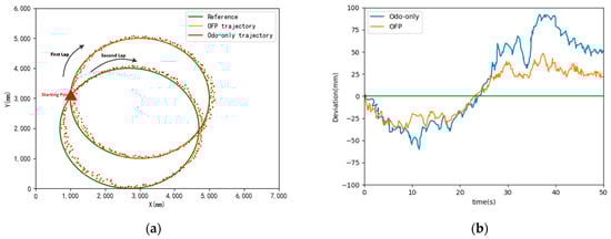
Figure 13.
Comparison of track deviation before and after odometry fusion. (a) Comparison trajectories before and after fusion. (b) Calculation of bias before and after fusion.
4.3.2. Joint Filter Positioning
Figure 14 presents the actual experimental results comparing the trajectories of odometer fusion positioning (OFP) and joint filter model fusion positioning (JFV) in Test Case 2. The figure contains three sets of curves corresponding to the three member robots. In Figure 14a, the mean deviation of the navigation trajectory using odometer fusion is 11.3 mm. Over time, the deviation of the RI developed trajectory shows a significant increasing trend due to cumulative errors in the internal sensors. In contrast, the joint-filtered navigation profile closely aligns with the reference trajectory without significant cumulative errors. Figure 14b showcases the trajectory comparison between the main robot’s odometer fusion localization (OFP) and joint-filtered model fusion localization (JFV). The JFV curve effectively mitigates the cumulative error observed in OFP.
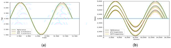
Figure 14.
Multi-robot system trajectory chart. (a) Trajectory of three member robots. (b) Trajectory of mail robot.
Figure 15 displays the peak curves derived from the trajectory deviations calculated during positioning experiments for both the main robot and the member robots. The JFV trajectory of the main robot exhibits greater accuracy compared with that of the member robots. This can be attributed to the main robot’s self-positioning in the global coordinate system, which experiences fewer observation errors. On the other hand, the global positioning of the member robots incorporates the observation errors of the main robot.
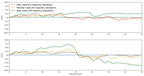
Figure 15.
Comparison of positioning error in Test Case 2.
4.3.3. Observation Occlusion Error Handling
The previous experimental procedure considered three error factors: target detection delay, network delay, and filter requirements for observation orientation. However, no treatment for masking observation errors has been applied. In this section, we use the experimental scenario of Test Case 3 to evaluate the masking error in observations. Theorem-type environments (including propositions, lemmas, corollaries, etc.) can be formatted as follows:
Figure 16 illustrates a scenario where the robot follows a small arc trajectory. R1 represents the main robot, while R2 and R3 are member robots. Throughout the motion, R3 remains obscured by R2 and cannot be observed by R1. The accuracy of R2, which relies on vision and laser navigation, is higher compared with that of R3, which relies on sonar array ranging data.
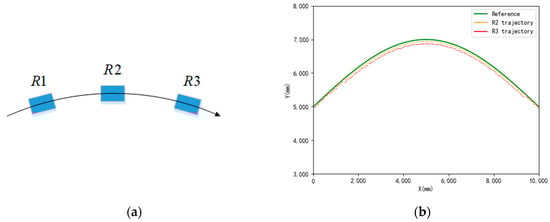
Figure 16.
Observation occlusion error handling. (a) Observation occlusion scene. (b) Track error handling.
5. Conclusions
This paper introduces a cooperative localization method based on a joint filtering model for practical multi-robot formation navigation. The method integrates sensor data from various sources to achieve precise localization. The model incorporates observation information from other robots, enhancing localization accuracy through cooperative efforts. The fusion of a laser rangefinder and vision sensor enables unique laser-ranging-based positioning by obtaining the target’s horizontal projection and the camera’s optical axis angle. Using a discrete Kalman filter to merge internal sensor data demonstrates superior real-time performance. The application of a visual target detection algorithm based on a convolutional neural network, along with visual and laser localization, employs a joint filtering model to fuse multiple sensors as a sub-filtering system. The resulting estimated deviation of robot position has a root mean square value of 22.8 mm in the x direction and 24.6 mm in the y direction, comparable to current research results based on collaborative autonomous SLAM positioning algorithms for multiple mobile robots that meet high accuracy requirements []. Moreover, it surpasses the co-localization errors of existing systems with multiple robot clusters in different formations. Lastly, an in-depth analysis of error sources is conducted in the actual formation application of a multi-robot system []. Experimental results demonstrate that the proposed positioning method achieves precise positioning with a small error range and negligible cumulative errors, making it suitable for real-world robot formation applications.
In our future work, we will engage in research in four challenging directions, including the improvement of navigation performance of multi-robot systems, formation control, and cooperative communication.
- (1)
- Leveraging current technology [], we aim to enhance and optimize our scheme. This involves addressing observation errors arising from the information fusion process and tackling time-delay errors in diverse formation configurations, varying robot numbers, and investigating different communication conditions. This challenging aspect contributes to the refinement of the existing architectural scheme.
- (2)
- We will examine the impact of applying the existing algorithms in height-transformed environments and develop 3D positioning information fusion schemes accordingly, which should enable a more accurate estimation of trip energy consumption to support some advanced future applications.
- (3)
- Based on the accurate position information of member robots and obstacles, the autonomous mobile robot group formation planning, holding, and control algorithms will be further investigated in combination with the currently available algorithmic models [,], and the optimal efficiency solution will be proposed based on different task scenarios.
- (4)
- It is necessary to conduct research on the interaction strategies of multi-robot systems under specific topologies and to design transmission strategies for the information in the interaction network, such as sensor data, communication protocols, control information, and images, which will meet the requirements of formation missions with high communication performance.
Author Contributions
Z.C. and J.L. conceived and designed the algorithm; Z.C. and W.C. performed the experiments; W.C. and B.Z. analyzed the data; and Z.C. and J.L. wrote the paper. All authors have read and agreed to the published version of the manuscript.
Funding
This research was supported in part by the sponsorship of the National Natural Science Foundation of China under Grant 42274051, in part by the Open foundation of Key Laboratory of Maritime Intelligent Cyberspace Technology, Ministry of Education under Grant MICT202306.
Data Availability Statement
Data are contained within the article.
Acknowledgments
The authors thank the Ministry of Science and Technology (MOST) for its financial support. We also thank the editor and anonymous reviewers for their constructive comments on this paper.
Conflicts of Interest
The authors declare no conflict of interest.
References
- Lupton, T.; Sukkarieh, S. Visual-Inertial-Aided Navigation for High-Dynamic Motion in Built Environments Without Initial Conditions. IEEE Trans. Robot. 2011, 28, 61–76. [Google Scholar] [CrossRef]
- Kelly, J.; Sukhatme, G.S. Visual-Inertial Sensor Fusion: Localization, Mapping and Sensor-to-Sensor Self-calibration. Int. J. Robot. Res. 2010, 30, 56–79. [Google Scholar] [CrossRef]
- Jones, E.S.; Soatto, S. Visual-inertial navigation, mapping and localization: A scalable real-time causal approach. Int. J. Robot. Res. 2011, 30, 407–430. [Google Scholar] [CrossRef]
- Shen, S. Autonomous Navigation in Complex Indoor and Outdoor Environments with Micro Aerial Vehicles; University of Pennsylvania ProQuest Dissertations Publishing: Philadelphia, PA, USA, 2014. [Google Scholar]
- Lu, Y.; Lee, J.; Yeh, S.H.; Cheng, H.M.; Chen, B.; Song, D. Sharing Heterogeneous Spatial Knowledge: Map Fusion Between Asynchronous Monocular Vision and Lidar or Other Prior Inputs. Robot. Res. 2019, 10, 727–741. [Google Scholar]
- Howard, A.; Matarić, M.J.; Sukhatme, G.S. Localization for Mobile Robot Teams: A Distributed MLE Approach. Exp. Robot. VIII 2003, 5, 146–155. [Google Scholar]
- Sun, R.; Yang, Y.; Chiang, K.-W.; Duong, T.-T.; Lin, K.-Y.; Tsai, G.-J. Robust IMU/GPS/VO Integration for Vehicle Navigation in GNSS Degraded Urban Areas. IEEE Sens. J. 2020, 20, 10110–10122. [Google Scholar] [CrossRef]
- Anbu, N.A.; Jayaprasanth, D. Integration of Inertial Navigation System with Global Positioning System using Extended Kalman Filter. In Proceedings of the International Conference on Smart Systems and Inventive Technology (ICSSIT), Tirunelveli, India, 27–29 November 2019; pp. 789–794. [Google Scholar]
- Mourikis, A.I.; Roumeliotis, S.I. A Multi-State Constraint Kalman Filter for Vision-aided Inertial Navigation. In Proceedings of the International Conference on Robotics and Automation, Rome, Italy, 10–14 April 2007; pp. 3565–3572. [Google Scholar]
- Dou, L.; Li, M.; Li, Y.; Zhao, Q.Y.; Li, J.; Wang, Z. A novel artificial bee colony optimization algorithm for global path planning of multi-robot systems. In Proceedings of the IEEE International Conference on Robotics and Biomimetics, Bali, Indonesia, 5–10 December 2014. [Google Scholar]
- Howard, A.; Matark, M.J.; Sukhatme, G.S. Localization for mobile robot teams using maximum likelihood estimation. In Proceedings of the IEEE International Workshop on Intelligent Robots and Systems (IROS), Lausanne, Switzerland, 30 September–4 October 2002. [Google Scholar]
- Chhatpar, S.R.; Branicky, M.S. Particle filtering for localization in robotic assemblies with position uncertainty. In Proceedings of the IEEE International Workshop on Intelligent Robots and Systems (IROS), Edmonton, AB, Canada, 2–6 August 2005. [Google Scholar]
- Burgard, W.; Cremers, A.B.; Fox, D.; Hähnel, D.; Lakemeyer, G.; Schulz, D.; Steiner, W.; Thrun, S. Experiences with an interactive museum tour-guide robot. Artif. Intell. 1999, 114, 3–55. [Google Scholar] [CrossRef]
- Fox, D.; Burgard, W.; Kruppa, H.; Thrun, S. A Probabilistic Approach to Collaborative Multi-Robot Localization. Auton. Robots 2000, 8, 325–344. [Google Scholar] [CrossRef]
- Rekleitis, I.M.; Dudek, G.; Milios, E.E. Multi-robot cooperative localization: A study of trade-offs between efficiency and accuracy. In Proceedings of the IEEE/RSJ International Conference on Intelligent Robots and Systems, Lausanne, Switzerland, 30 September–4 October 2002. [Google Scholar]
- Ning, B.; Han, Q.L.; Zuo, Z.; Jin, J.; Zheng, J. Collective Behaviors of Mobile Robots Beyond the Nearest Neighbor Rules With Switching Topology. IEEE Trans. Cybern. 2017, 48, 1577–1590. [Google Scholar] [CrossRef] [PubMed]
- Shucker, B.; Murphey, T.; Bennett, J.K. A method of cooperative control using occasional non-local interactions. In Proceedings of the 2006 IEEE International Conference on Robotics and Automation (IRCA), Orlando, FL, USA, 15–19 May 2006. [Google Scholar]
- Garcia, M.A.; Solanas, A. 3D simultaneous localization and modeling from stereo vision. In Proceedings of the IEEE International Conference on Robotics and Automation (IRCA), New Orleans, LA, USA, 26 April–1 May 2004. [Google Scholar]
- Kannala, J.; Heikkilä, J.; Brandt, S.S. Geometric Camera Calibration. Wiley Encycl. Comput. Sci. Eng. 2008, 13, 1–20. [Google Scholar]
- Zong, G.; Deng, L.; Wang, W. Robust Localization algorithms for outdoor mobile robot. J. Beijing Univ. Aeronaut. Astronaut. 2007, 33, 454–458. [Google Scholar]
- Wang, C.Y.; Bochkovskiy, A.; Liao, H.Y. Scaled-YOLOv4: Scaling Cross Stage Partial Network. In Proceedings of the IEEE/CVF Conference on Computer Vision and Pattern Recognition (CVPR), Nashville, TN, USA, 20–25 June 2021; pp. 13029–13038. [Google Scholar]
- Wang, C.Y.; Liao, H.Y.; Wu, Y.H.; Chen, P.Y.; Hsieh, J.W.; Yeh, I.H. CSPNet: A New Backbone That Can Enhance Learning Capability of CNN. In Proceedings of the IEEE/CVF Conference on Computer Vision and Pattern Recognition (CVPR) Workshops, Seattle, WA, USA, 13–19 June 2020; pp. 390–391. [Google Scholar]
- Hu, G.X.; Yang, Z.; Hu, L.; Huang, L.; Han, J.M. Small Object Detection with Multiscale Features. Int. J. Digit. Multimed. Broadcast. 2018, 2018, 4546896. [Google Scholar] [CrossRef]
- Jilkov, V.P.; Angelova, D.S.; Semerdjiev, T.A. Design and comparison of mode-set adaptive IMM algorithms for maneuvering target tracking. IEEE Trans. Aerosp. Elecreonis Syst. 1999, 35, 343–350. [Google Scholar] [CrossRef]
- Wang, L.; Liu, Y.H.; Wan, J.W.; Shao, J.X. Multi-Robot Cooperative Localization Based on Relative Bearing. Chin. J. Sens. Actuators 2007, 20, 794–799. [Google Scholar]
- Wang, J. Multi-Robot Collaborative SLAM Algorithm Research. Master’s Thesis, Xi’an University of Technology, Xi’an, China, 2023; pp. 47–63. [Google Scholar]
- Zhu, K.; Wen, Z.; Di, S.; Zhang, F.; Guo, G.; Kang, H. Observability and Co-Positioning Accuracy Analysis of Multi-Robot Systems. Telecommun. Eng. 2023, 51, 4–8. [Google Scholar]
- Chiang, K.W.; Duong, T.T.; Liao, J.K. The Performance Analysis of a Real-Time Integrated INS/GPS Vehicle Navigation System with Abnormal GPS Measurement Elimination. Sensors 2013, 13, 10599–10622. [Google Scholar] [CrossRef] [PubMed]
- Yang, S.; Li, T.; Shi, Q.; Bai, W.; Wu, Y. Artificial Potential-Based Formation Control with Collision and Obstacle Avoidance for Second-order Multi-Agent Systems. In Proceedings of the 2020 7th International Conference on Information, Cybernetics, and Computational Social Systems (ICCSS), Guangzhou, China, 13–15 November 2021. [Google Scholar]
- Lu, Q.; Han, Q.L.; Zhang, B.; Liu, D.; Liu, S. Cooperative Control of Mobile Sensor Networks for Environmental Monitoring: An Event-Triggered Finite-Time Control Scheme. IEEE Trans. Cybern. 2016, 47, 4134–4147. [Google Scholar] [CrossRef] [PubMed]
Disclaimer/Publisher’s Note: The statements, opinions and data contained in all publications are solely those of the individual author(s) and contributor(s) and not of MDPI and/or the editor(s). MDPI and/or the editor(s) disclaim responsibility for any injury to people or property resulting from any ideas, methods, instructions or products referred to in the content. |
© 2023 by the authors. Licensee MDPI, Basel, Switzerland. This article is an open access article distributed under the terms and conditions of the Creative Commons Attribution (CC BY) license (https://creativecommons.org/licenses/by/4.0/).