Research on the Characteristic Spectral Band Determination for Water Quality Parameters Retrieval Based on Satellite Hyperspectral Data

Abstract

Hyperspectral remote sensing technology has been widely used in water quality monitoring. However, while it provides more detailed spectral information for water quality monitoring, it also gives rise to issues such as data redundancy, complex data processing, and low spatial resolution. In this study, a novel approach was proposed to determine the characteristic spectral band of water quality parameters based on satellite hyperspectral data, aiming to improve data utilization of hyperspectral data and to achieve the same precision monitoring of multispectral data. This paper first introduces the data matching method of satellite hyperspectral data and water quality based on space–time information for guidance in collecting research data. Secondly, the customizable and fixed spectral bands of the existing multispectral camera products were studied and used for the preprocessing of hyperspectral data. Then, the determination approach of characteristic spectral bands of water quality parameters is proposed based on the correlation between the reflectance of different bands and regression modeling. Next, the model performance for retrieval of various water quality parameters was compared between the typical empirical method and artificial neural network (ANN) method of different spectral band sets with different band numbers. Finally, taking the adjusted determination coefficient $\overline{R^2}$ as an evaluation index for the models, the results show that the ANN method has obvious advantages over the empirical method, and band set providing more band options improves the model performance. There is an optimal band number for the characteristic spectral bands of water quality parameters. For permanganate index (COD_Mn), dissolved oxygen (DO), and conductivity (EC), the $\overline{R^2}$ of the optimal ANN model with three bands can reach about 0.68, 0.43, and 0.49, respectively, whose mean absolute percentage error (MAPE) values are 14.02%, 16.26%, and 17.52%, respectively. This paper provides technical guidance for efficient utilization of hyperspectral data by determination of characteristic spectral bands, the theoretical basis for customization of multispectral cameras, and the subsequent water quality monitoring through remote sensing using a multispectral drone.

1. Introduction

Remote sensing has the advantage of large-scale, all-weather accurate dynamic monitoring, and has been widely used in the water conservancy industry. Remote sensing of the water environment was born, and its development has kept pace with the times [1]. Changes in the composition and concentration of substances in the water often cause changes in the color of the water body [2]. Remote sensing technology of spectral imaging can obtain the color parameters of the water body by obtaining the spectral characteristics of the water body, and then inverse the water quality parameters, so as to realize the water environment monitoring of rivers and lakes [3,4].

Most applications of remote sensing monitoring technology and spectral imaging in the field of water environment monitoring can be summarized in three steps: remote sensing data acquisition, data processing and inversion model construction, and model analysis and application. The available data sources for remote sensing of water quality retrieval are usually multispectral and hyperspectral remote sensors [5] categorized by the spectral resolution of the sensors, carried by the spaceborne, airborne, and portable and ground-based load platforms [6]. Multispectral data available for remote sensing water quality retrieval typically have 3–10 bands. Landsat series data are the most commonly utilized for water quality monitoring, such as TSM, COD, and TP, due to their accessibility and geographic, temporal, and spectral resolution [7,8]. Hyperspectral satellites have multiple bands with about 5–10 nm spectral resolution. For retrieving water quality, hyperspectral data from satellites such as the HuanJing-1 (HJ-1) [9], Gaofen-5 (GF-5) [10], and Ziyuan1-02D (ZY1-02D) [11] have been employed. Higher spectral resolution data have a large number of bands that can be precisely and optimally chosen for developing inversion models of water quality parameters to differentiate the spectral differences in multispectral data, greatly enhancing the accuracy of inversion algorithms [12,13,14]. Among the four spectral sensor platforms for the water quality monitoring, the portable and ground-based spectrometer [4] is less flexible and more labor-intensive; the airborne spectrometer [5,6] is flexible and has high spatial resolution, but the observation area is small; and the satellite-based spectrometer [8] has low imagery cost and is suitable for large-scale monitoring, but it has the disadvantages of low spatial resolution, poor timeliness, and long revisit cycle.

In terms of model construction for water quality parameter retrieval, it is mainly divided into the empirical method, analytical method (also called bio-optical method [6]), artificial intelligence (AI) method, and combined empirical and analytical methods. The fourth method is called the semi-empirical model or semi-analytical model, while in some studies they were listed together [6]. The empirical method relies only on the statistical relationship between remote sensing data and measured water quality parameters to establish models [15,16,17,18]. The principle of the model is simple and the accuracy of the results is high, but the generality of the results is low. The analysis model is based on the principle of water radiative transfer, and the content of each component in the water is calculated from the remote sensing data through the transfer formula [19]. For example, Dekker et al. [20] estimated the water color parameters by building a physical analysis model based on Landsat TM data and the measured intrinsic optical quantity of the water body. Sudduth et al. [12] used airborne hyperspectral data images of the major rivers in Minnesota to establish an analysis model, which was based on the intrinsic optical quantity of the water body and the apparent optical quantity calculated from the spectral data, thereby retrieving the suspended solids concentration of the river and noting that 700 nm is the best band for measuring the suspended solids concentration in the study area. This type of model has good universality and high precision, but the model is difficult to fit. The physical meaning of the spectral index used in the semi-empirical model is clearer than that used in the empirical method. Taking the concentration of chlorophyll-a as an example, the semi-empirical model method is to propose the spectral index related to its concentration based on certain assumptions related to the bio-optical theoretical model [21], and establish a statistical relationship to realize the inversion of the water quality parameters [22,23]. The construction of the analytical model depends on the complex water radiative transfer model, and the existing analytical models almost need to introduce empirical formulas to determine some parameters. Generally, the analytical model with empirical formulas is called the semi-analytical model [24,25], which requires the measured absorption coefficient and other intrinsic optical parameters. The AI model effectively trains a large number of reflectivity and water quality parameters by using an AI algorithm, and automatically learns the nonlinear relationship between the two through the network to realize the prediction of water quality parameters [5,26,27,28].

The core of modeling various water quality parameters is band selection and band combination [29]. In the past, multispectral data were the main data used for water environment remote sensing, and only a few bands could not accurately obtain the spectral information of different water quality parameters. In recent years, the number of satellites equipped with hyperspectral imagers has gradually increased, such as ZY1-02D [11], GF-5 [30], and the Hyperspectral Precursor and Application Mission (PRISMA) [31]. The on-board hyperspectral camera provides a broad data source for hyperspectral data acquisition, and hyperspectral remote sensing data also provides more bands for model building [32]. The spectral curve for water elements also obtained provides a basis for analyzing the physical meaning of bands, and can help researchers to establish a more accurate semi-empirical model with clearer physical meaning. However, the number of hyperspectral remote sensing bands is usually hundreds. At this stage, the band utilization efficiency of the semi-empirical inversion model is generally low. In general, the establishment of the target water quality parameter inversion model can only be completed with data within four bands, resulting in new problems such as hyperspectral data redundancy and complex processing. Therefore, based on the analysis of spectral characteristics of water elements, the band or band combination can be reasonably selected, and a superior semi-empirical retrieval model of hyperspectral water elements can be constructed to guide the customization of the multispectral camera, so as to realize the same precision inversion of water quality parameters based on the customized multispectral camera. At the same time, there are still some limitations in spaceborne hyperspectral technology, such as the spatial resolution, which creates difficulties in monitoring small lakes, reservoirs, and other small water areas, and there are restrictions on the acquisition of some commercial satellite data. Unmanned aerial vehicles (UAVs) [33] have the advantages of low cost, simple operation, high spatial resolution, and easy realization of scanning and imaging. It is convenient for field operation to patrol the water environment, which can effectively overcome this disadvantage. In summary, for the retrieval of water quality parameters, hyperspectral data have the disadvantages of low spatial resolution, excessive data redundancy, low data utilization, and only a few bands are used in the inversion model. Therefore, it is necessary to determine the method of identifying the characteristic bands of the satellite hyperspectral data inversion model, and realize monitoring at the same accuracy with multispectral data as the hyperspectral data. The follow-up research can be used to guide the effective band customization of the multispectral lens used for UAVs, and realize high-resolution, efficient, flexible, fast and low-cost water environment inspection of small water areas by combining the flexibility of UAVs, the characteristics of efficient data utilization, and the low cost of a multispectral lens.

Li et al. [32] utilized hyperspectral data from the Gaofen-5 satellite and employed machine learning methods to comprehensively characterize the features of the hyperspectral data through the combination of multispectral-scale morphological features. They investigated the relationship between the hyperspectral data and water quality parameters, and established a retrieval model. However, this study did not explore efficient utilization methods for hyperspectral data or redundant data removal techniques. Zheng et al. [11], on the other hand, used hyperspectral data from the ZY1-02D satellite and developed a water quality inversion model using machine learning techniques. They utilized empirical parameters and the ratio between two bands as inputs. The focus of their study was primarily on examining the impact of different machine learning methods and comparing the performance of ZY1-02D satellite hyperspectral data with Sentinel-2 multispectral data. Although both studies employed machine learning (AI) methods to construct water quality parameter inversion models, they did not specifically investigate characteristic spectral bands for water quality parameters. These characteristic bands are often derived through empirical models and have certain limitations.

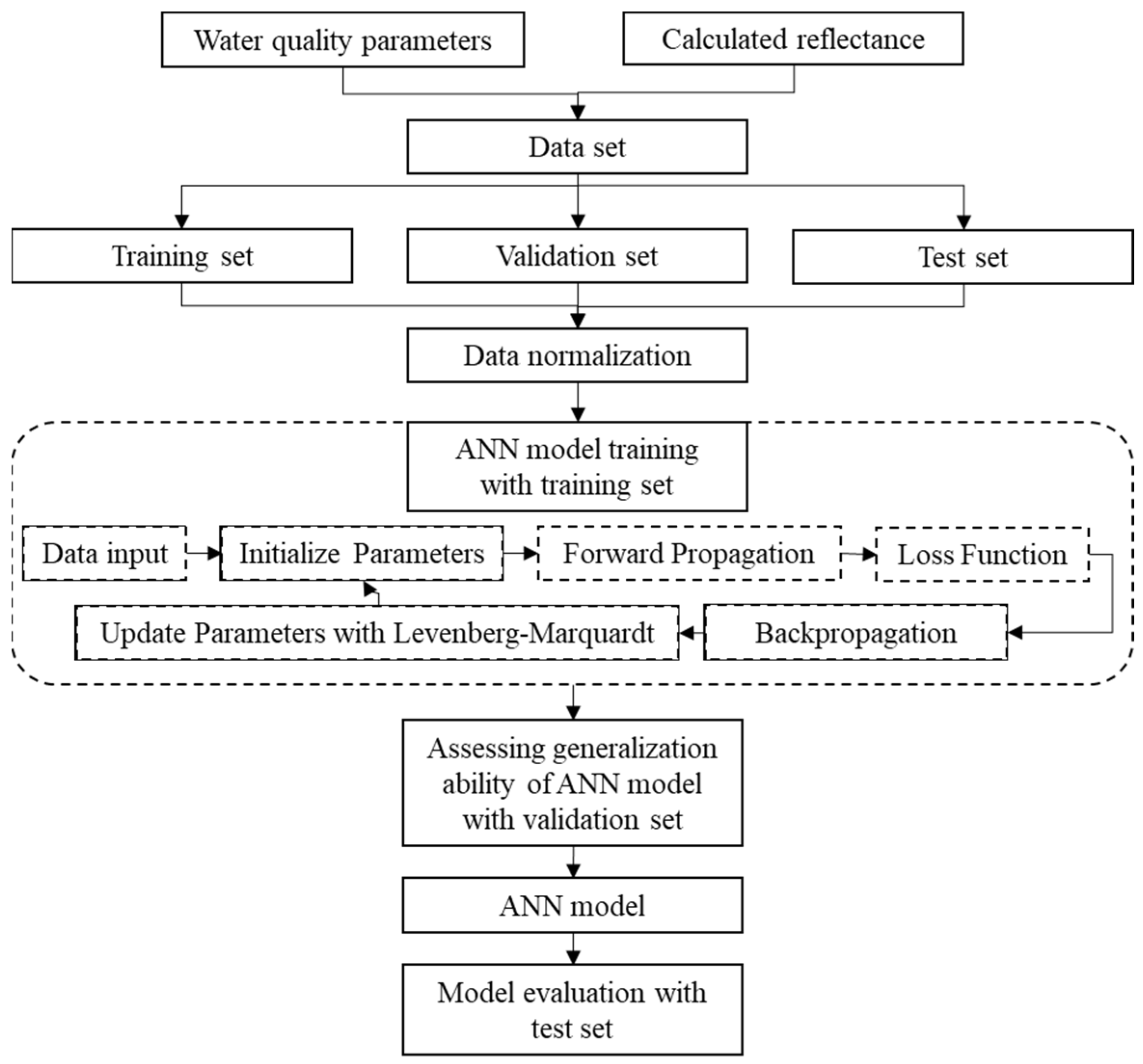
Therefore, this paper aims to combine the advantages of AI algorithms and the explicit concept of characteristic spectral bands for water quality parameters. Based on hyperspectral data from the ZY1-02D satellite, the objective of this paper is to compare the model performance for retrieving various water quality parameters between the typical empirical method and artificial neural network (ANN) method by using different spectral band sets with different band numbers, so as to provide a guidance approach for the determination of characteristic bands of different water quality parameters. This article first introduces the research area and data sources together with the matching method for quality parameters and satellite hyperspectral data to collect data. Then, the preprocessing methods for water quality data and hyperspectral data are introduced. Then, the method for determining the characteristic spectral bands of water quality parameters is highlighted and derived from the correlation of band reflectance and the regression model methods based on empirical and ANN methods. The Results section introduces the high correlation of the two bands and the reduced computational complexity, along with the results of the empirical method-based model and the ANN-based model. The Discussion section provides recommended values for customizing the characteristic bands and directions for improving the model. Figure 1 is the overall technical flowchart for this work.

2. Materials

2.1. Study Area

As shown in Figure 2, this study selected the areas around Taihu Lake, such as Suzhou, Wuxi, Shanghai, Jiaxing, and Huzhou, as the region to collect water quality and satellite data. The water network in this region is dense; the distribution of National Surface Water Automatic Monitoring Stations (NSWAMS) stations is concentrated and dense, which can effectively improve the utilization rate for the satellite data. Water quality parameters used in this paper were acquired for the period December 2020 to August 2022.

2.2. Data Collection

The water quality parameters are from the National Surface Water Automatic Monitoring Real-Time Data Release System of the China Environmental Monitoring Station. The release scope of this system includes data from the National Surface Water Automatic Monitoring Stations (NSWAMS) system, which was built and officially put into operation. From April 2014 to November 2020, NSWAMS included 134 stations. In December 2020, 1506 new stations were added. In 2021, 365 new stations were added. Currently, there are a total of 2005 stations, which can provide sufficient data support for building regression models of satellite hyperspectral data and water quality parameters.

The water parameters released include water temperature, pH, dissolved oxygen (DO), permanganate index (COD_Mn), ammonia nitrogen (NH3-N), total phosphorus (TP), total nitrogen (TN), electric conductivity (EC), and turbidity (TUB), a total of 9 monitoring indicators. The data are released every 4 h, which can effectively correspond to the satellite transit at different times. This paper selects 7 water quality parameters as research objects: DO, COD_Mn, NH3-N, TP, TN, TUB, and EC.

The hyperspectral satellite data comes from the Natural Resources Satellite Remote Sensing Cloud Service Platform, and are obtained from the hyperspectral camera on the ZY1-02D satellite, the Advanced Hyperspectral Imager (AHSI) sensor [11]. It has been shown that for the AHSI hyperspectral sensor, the average equivalent reflectance for each band in situ R_rs and the multispectral sensor Multispectral Imager (MSI) are basically the same [11]. The satellite carries two cameras that can effectively obtain 9-band multispectral data with 115 km width and 166-band hyperspectral data with 60 km width. Among them, the full spectral resolution can reach 2.5 m; the multispectral is 10 m and the hyperspectral is 30 m. The visible near infrared and shortwave infrared spectral resolution of the hyperspectral payload can reach 10 and 20 nm, respectively. The main parameters of the AHSI are shown in

Table 1. Main parameters of the ZY1-02D satellite hyperspectral camera.

Spectral Range	Spatial Resolution	Spectral Resolution		Width
		Visible/Near Infrared	SWIR
0.4–2.5 μm, 166 spectral bands	30 m	10 nm	20 nm	60 km

.

The hyperspectral data from the ZY1-02D satellite have been radiometrically corrected, bad pixels repaired, and spectrally calibrated. To meet the application requirements of quantitative remote sensing, radiometric calibration, atmospheric correction, and orthorectification must be performed [11], as shown in Figure 3. Among them, orthorectification is performed by using the built-in RPC file and Landsat 8 data after terrain correction as a reference image. One example of the ZY1-02D satellite image products is shown in Figure 4, in which the detailed information was listed including the produce time, longitude and latitude, and so on.

3. Method

In this section, we introduce the methodology employed in this paper, which includes data matching, data processing, determination of characteristic spectral bands, regression modeling, and model evaluation. The water quality parameters and hyperspectral data do not possess a direct one-to-one correspondence; the data matching method is to establish a consistent correspondence between water quality data collected at the same geographical location and time and the corresponding satellite hyperspectral data. Preprocessing of the water quality parameters and hyperspectral satellite data is necessary to normalize the distribution of the water quality parameters and ensure the hyperspectral data are processed within the spectral range of interest specific to this paper. The determination of characteristic spectral bands represents a crucial innovation in this research, allowing for efficient selection of relevant bands for different water quality parameters through correlation analysis with a regression model. Various regression modeling methods are presented in this section to evaluate and compare their performance in modeling, and to determine the optimal approach for regression modeling between the water quality parameters and calculated reflectance. Model evaluation is necessary to clearly elaborate the specific parameters used to compare different regression models and to specify the calculation formulas for these comparison metrics.

3.1. Data Matching of Water Quality Parameters and Hyperspectral Satellite Data

The data matching method integrates geometric and temporal information to establish correspondence between water quality parameters and hyperspectral satellite data, enabling the spectral characteristics from the satellite data to represent the water quality parameters.

This paper realizes the heterogeneous data matching of water quality monitoring data and ZY1-02D satellite hyperspectral data of the same NSWAMS based on the location and time, whose principle is shown in Figure 5. Twenty scenes of hyperspectral data with the highest utilization rate were selected as the research data of this paper.

The specific methods are shown in Figure 6, as follows:

(1) Data extraction for a range of locations and times. On the Natural Resources Satellite Remote Sensing Cloud Service Platform, the time condition is “December 2020–August 2022”, the geographical conditions are Suzhou, Shanghai, Jiaxing, Huzhou, and Wuxi, the satellite sampling conditions are the AHSI sensor of ZY1-02D and 0 cloud amount; a total of 61 scenes were found, of which 8 scenes had low-altitude cloud phenomenon, so 53 scenes were available for selection. Water quality monitoring data were obtained from each NSWAMS in Suzhou, Shanghai, Jiaxing, Huzhou, and Wuxi from December 2020 to August 2022 from the National Surface Water Automatic Monitoring Real-Time Data Release System. Each datum includes the name, time, water quality classification, temperature, pH, DO, COD_Mn, NH3-N, TP, TN, EC, and TUB of the NSWAMS, together with latitude and longitude;

(2) Determination if each NSWAMS is within the satellite data. For the ith scene of the hyperspectral satellite data sh_i, the sampling date and time is t_i, the four vertices are a_i, b_i, c_i and d_i, whose latitudes and longitudes are (lon_ai, lat_ai), (lon_bi, lat_bi), (lon_ci, lat_ci), and (lon_di, lat_di). Assuming that the water quality parameter set rwq_i was collected at the same sampling time t_i, and that the number of water quality parameters records in this set is n_i, the latitude and longitude of the NSWAMS e_i,j corresponding to the jth water quality parameter record rwq_i,j is (lon_ei,j, lat_ei,j), where $\mathrm{j}\in \left\{\mathrm{1,2},3,...,\mathrm{n}\right\}$. The area method is used to determine if this NSWAMS is within the satellite hyperspectral data of this scene. The area of the parallelogram formed by a_i, b_i, c_i, and d_i is s_i, and e_i,j forms four triangles with each side of the quadrangle area, whose areas are s_i,j,1, s_i,j,2, s_i,j,3, and s_i,j,4, respectively. If s_i is less than the sum of the four areas noted, then it proves that the NSWAMS is within the scene data, and these water quality parameter records are collected in the selected set swq_i. Otherwise, if it is higher, it is outside the hyperspectral satellite data of this scene. If the NSWAMS is determined to be within the geographic location of the ith satellite data according to the method described above, then the water quality parameter records within the satellite data are collected into the dataset swq_i.

(3) Selection of satellite data with the top 20 water quality parameter records. The number of water quality parameter records in this dataset is calculated, which is the number of NSWAMS in this satellite scene num_i. The number of NSWAMS in each scene of satellite data is calculated using on the method described above, and the numbers of water quality parameter records of all scenes are sorted. The 20 scenes of satellite data with the highest number of NSWAMS are taken for analysis, which are the 20 scenes of satellite hyperspectral data with the highest effective information density;

(4) Extraction of spectral value curve corresponding to each water quality parameter sample. According to the geographic information for the NSWAMSs collected from each scene, ENVI 5.3 software is used to extract the entire spectral value curve for the water body at the corresponding position in the hyperspectral satellite image, the spectral mean of scale 1 is taken as the spectral value [20].

All of the water quality parameter records and the spectral curves for the water body with the same position and time are collected. Using these methods, 188 records of water quality parameters at different times and locations and their corresponding satellite hyperspectral data in time and space were obtained, realizing the matching of 20 scenes of satellite hyperspectral data with the highest effective information density together with their water quality parameters.

3.2. Data Preprocessing

3.2.1. Water Quality Data Preprocessing

According to the Environmental Quality Standards for Surface Water (GB3838-2002), the classification criteria for Class I-V waters with DO, COD_Mn, NH3-N, TP, and TN are shown in

Table 2. Classification criteria for water quality parameters.

No.	Parameters	Class I	Class II	Class III	Class IV	Class V
1	DO≥	7.5	6	5	3	2
2	CODMn≤	2	4	6	10	15
3	NH3-N≤	0.15	0.5	1	1.5	2
4	TP≤	0.02	0.1	0.2	0.3	0.4
5	TN≤	0.2	0.5	1	1.5	2

.

According to these classification criteria, the water classification distribution for the 188 records of various water quality parameters is shown in Figure 7a.

It can be seen from Figure 7a that there is a phenomenon of excessive concentration in the distribution of each water quality parameter within a certain interval. For example, the proportion of class I DO is 78.27%, the class II proportion of COD_Mn is 63.83%, the sum class I and class II proportion of NH3- N is above 40%, the class II and class III proportion of TP is 51.60% and 37.23%, respectively, and the class V proportion of TN is 53.19%. In order to ensure the accuracy and generalization for the inversion results of various water quality parameters, it is necessary to ensure that each parameter is evenly distributed within each classification interval as much as possible to reduce the phenomenon of distribution concentration. The priority is given to removing data points that simultaneously include Class I DO, Class II COD, Class I or II NH3-N, Class II TP, and Class V and inferior TN. After analysis and screening, 90 records of water quality parameters were selected, and the water classification distribution for each water quality parameter is shown in Figure 7b.

As a result, the water quality monitoring data in relatively concentrated intervals were essentially deleted, resulting in a relatively uniform distribution.

Table 3. Number of different classifications of various water quality parameters after screening.

Statistical Value	DO	CODMn	NH3-N	TP	TN	EC	TUB
Mean	8.26	3.95	0.35	0.110	2.42	511	80.6
Min	1.32	1.62	0.03	0.005	0.20	155	2.5
Max	15.79	9.46	1.41	0.649	9.25	1020	255.9
Std	2.74	1.43	0.33	0.087	1.79	158	59.1

shows the descriptive statistics of various water quality parameters for the 90 records.

3.2.2. Hyperspectral Satellite Data Preprocessing

The purpose of this paper is to determine the characteristic spectral bands of different water quality parameters, so as to provide the theoretical basis and application guidance for the band customization of the multispectral camera suitable for drones. The spectral range of interest is from the existing multispectral cameras and customizable multispectral cameras suitable for drones, as follows.

At present, there are many institutions engaged in the development of UAV multispectral imaging equipment, and the multispectral cameras in existing UAVs are mainly used for agricultural crop growth assessment, plant classification, forestry monitoring, etc., as shown in

Table 4. Index parameters of existing multispectral cameras for drones.

No.	Institutions	Product Name	Spectral Channel Numbers	Spectral Channel Bands Information
1	Parrot (France)	SEQUOIA	4 multispectral channels + 1 RGB channel	550 nm@40 nm, 660 nm@40 nm, 735 nm@10 nm, 790 nm@40 nm
2	Micasense (USA)	RedEdge-MX	5 multispectral channels	475 nm@32 nm, 560 nm@27 nm, 668 nm@16 nm, 717 nm@12 nm, 842 nm@57 nm
3	Yusense (China)	MS600 Pro	6 multispectral channels	450 nm@35 nm, 555 nm@27 nm, 660 nm@22 nm, 720 nm@10 nm, 750 nm@10 nm, 840 nm@30 nm
4	Yusense (China)	AQ600 Pro	5 multispectral channels + 1 RGB channel	450 nm@35 nm, 555 nm@27 nm, 660 nm@22 nm, 720 nm@10 nm, 840 nm@30 nm
5	DJ (China)	Phantom 4 multispectral version	5 multispectral channels + 1 RGB channel	450 nm@16 nm, 560 nm@16 nm, 650 nm@16 nm, 730 nm@16 nm, 840 nm@26 nm
6	DJ (China)	Mavic3 multispectral version	4 multispectral channels + 1 RGB channel	560 nm@16 nm, 650 nm@16 nm, 730 nm@16 nm, 860 nm@26 nm

.

The 6 channels and 5 channels of MS600 Pro and AQ600 Pro, respectively, are customizable. The customizable spectral channels include 16 bands with different wavelengths, i.e., 410 nm@35 nm, 450 nm@35 nm, 490 nm@25 nm, 530 nm@27 nm, 555 nm@27 nm, 570 nm@32 nm, 610 nm@30 nm, 650 nm@27 nm, 660 nm@22 nm, 680 nm@25 nm, 720 nm@10 nm, 750 nm@10 nm, 780 nm@13 nm, 800 nm@35 nm, 840 nm@30 nm, and 900 nm@35 nm. The products that realize the integration of the drone body and multispectral camera are the DJ Phantom 4 multispectral version and the DJ Mavic3 multispectral version. The index parameters of the two products are shown in Table 4.

Since the maximum band wavelength of the customized UAV multispectral camera is 900 nm, the 166 bands with the wavelength from 396 nm to 2501 nm are first deleted to 60 bands with the wavelength from 396 to 903 nm. The obtained spectral curves for different collected hyperspectral satellite data are shown in Figure 8. In Figure 8, the y-axis is the remote sensing reflectance and the x-axis is the center wavelength value of the spectral channel bands. It can be seen from Figure 7 that there is a peak in the wavelength range from 550 to 580 nm for the reflectance, which increases sharply between 390 and 580 nm, but some of them are decreased in the wavelength range from 390 to 490 nm. Then, the reflectance increases from 490 to 580 nm, and generally decreases from 580 to 756 nm. There is a small peak in reflectance at 765 nm. For the remaining wavelength range, the regular pattern is not obvious, generally maintaining the level of fluctuation or slightly decreasing.

In this paper, the customizable 16 spectral band combination set is referred to as CM16, and the spectral band combination set of other existing products is referred to as the product name. For example, the 4-multispectral band combination for Parrot multispectral cameras is referred to as the Par set, and so on. The band set name and spectral information of the band set are shown in

Table 5. Information for different multispectral band combination sets.

No.	Band Set Name	Center Wavelengths of Bands in the Band Set (nm)
1	Par	550, 660, 735, 790
2	Mic	475, 560, 668, 717, 842
3	DJ3	560, 650, 730, 860
4	DJ4	450, 560, 650, 730, 840
5	MS600	450, 555, 660, 720, 750, 840
6	AQ600	450, 555, 660, 720, 840
7	CM16	410, 450, 490, 530, 555, 570, 610, 650, 660, 680, 720, 750, 780, 800, 840, 900

.

In order to compare the inversion performance of the above 7 band sets on 7 different water quality parameters and to determine the characteristic spectral bands of each parameter, the following section describes the empirical and artificial neural network (ANN) methods used to fit the reflectance data for single-band, two-band combinations, and three-band combinations from the above 7 band sets with water quality parameters, and to determine the optimal 6 spectral band combinations based on the obtained characteristic spectral bands for each water quality parameter in the customization of a 6-band multispectral camera. To achieve this goal, a total of 26 bands involved in the above 7 band sets were first determined. Then, the reflectance at the corresponding wavelengths of the 26 bands was calculated using the interpolation method. Finally, the remaining bands were deleted, and the preprocessing of the hyperspectral data was completed. The spectral curves for the 26 bands are shown in Figure 9.

3.3. Determination of Characteristic Spectral Bands for Water Quality Parameters Based on the Correlation between Reflectance of Different Bands

From the perspective of water quality parameter measurement, the effective utilization of hyperspectral data leads to selection of the characteristic spectral band combinations for different water quality parameters. By using multiple characteristic bands, accurate inversion of each water quality parameter can be achieved, which can ensure the accuracy of water quality parameter measurement and the simplicity of spectral bands, remove redundant data, improve spectral data processing speed, and achieve efficient utilization of spectral data.

This paper proposes a method to determine the optimal characteristic bands based on the reflectance correlation of different bands, which is shown in Figure 10. For the given band set, the number of bands contained in the band set is n_bs. The steps of the approach follow.

(1) Determination of a high correlation two-band set. The determination coefficient $R^2$ [26] between the reflectance data corresponding to each two-band combination in a given band set was calculated by Equation (1).

$$R^2=1-\frac{{\sum }_{i=1}^n{\left(R_{rs,i}^A-R_{rs,i}^B\right)}^2}{{\sum }_{i=1}^n{\left(R_{rs,i}^A-{\overline{R}}_{rs}^A\right)}^2}$$

(1)

where n is the number of the reflectance data samples, $R_{rs}^A$represents the reflectance data corresponding to band A, and $R_{rs}^B$represents the reflectance data corresponding to band B.

The two bands with the determination coefficient $R^2$ greater than 0.9 were considered to have the same effect in the same characteristic spectral band combination. Therefore, they cannot appear simultaneously in a characteristic spectral band combination containing two or more bands [34]. The dataset of the two-band combinations with $R^2$ higher than 0.9 is expressed as S.

The maximum number of spectral bands n_bmax contained in a spectral band combination and the number of different spectral band combinations with different numbers of bands could also be determined so that the spectral band combination cannot contain the two highly correlated bands.

(2) Calculated reflectance of the spectral band combination without high correlation between two bands. For the cith spectral band wavelength combination $S_{n_b,ci}$, consisting of the ith, jth, …, and zth bands wavelength, $\left({\lambda }_{ii},{\lambda }_{jj}\right)$represents arbitrary wavelength combination of two bands from $S_{n_b,ci}$. If $\left({\lambda }_{ii},{\lambda }_{jj}\right)$ does not belong to the dataset S, then the reflectance data corresponding to the wavelengths in the spectral band combinations $S_{n_b,ci}$ can be used to calculate the combination reflectance $R_{n_b,ci}$ with Equation (2).

$$R_{n_b,ci}=f\left(R\left({\lambda }_{i,1}\right),R\left({\lambda }_{j,2}\right),\dots ,R\left({\lambda }_{z,n_b}\right)\right)$$

(2)

The definition and restriction conditions of the notations are listed in

Table 6. Definition and restriction conditions of the notations.

Notations	Definition	Restriction Conditions
$S_{n_b,ci}$	The cith spectral band wavelength combination	$S_{n_b,ci}=\left\{{\lambda }_{i,1},{\lambda }_{j,2},\dots ,{\lambda }_{z,n_b}\right\}$ $ci\in \left\{\mathrm{1,2},3,\dots ,n_c\right\}$
i,j,…,z	The ith, jth, …, and zth band wavelength	$i\ne j\ne ,\dots ,\ne z$ $i\notin \left\{\mathrm{1,2},3,\dots ,n-n_b+1\right\}$ $j\notin \left\{\mathrm{2,3},\dots ,n-n_b+2\right\}$ $z\notin \left\{n_b,n_b+1,n_b+2,\dots ,n\right\}$
nb	The number of bands included in the combination $S_{n_b,ci}$	$n_b\in \left\{\mathrm{1,2},3,\dots ,n_{bmax}\right\}$
nc	The number of the maximum value of the combinations with nb bands	$n_c=C_{n_{bs}}^{n_b}$
$\left({\lambda }_{ii},{\lambda }_{jj}\right)$	Arbitrary wavelength combination of two bands from $S_{n_b,ci}$	${\lambda }_{ii},{\lambda }_{jj}\in S_{n_b,ci}$ $ii\ne jj$
$R_{n_b,ci}$	Calculated reflectance of spectral band combination without high correlation two bands	-

.

(3) Characteristic spectral bands determination. The combination reflectance $R_{n_b,ci}$ corresponding to the spectral band combinations $S_{n_b,ci}$ containing one to n_bmax bands that meet the requirements were traversed to build the regression models with the selected method for inversion with different water quality parameters. The models with the best performance are used to determine the different characteristic spectral band combinations and the number of bands included in the combinations for different water quality parameters. Using the same method mentioned above, other band sets Par, Mic, DJ3, DJ4, MS600, and AQ600 were fitted, and the characteristic spectral band combination for each water quality parameter was selected. The band set that can achieve optimal results was determined by comparing the performance of different band combination models. The characteristic spectral bands of each water quality parameter were summarized within the optimal band set.

(4) Optimal spectral bands selection. By ensuring accurate monitoring of the required water quality parameters while satisfying the overall band quantity requirement, the optimal spectral bands were selected based on the specific monitoring requirements for water quality parameters and the total number of bands that was needed. This approach aimed to achieve precise remote sensing measurements of water quality parameters within the specified number of bands.

3.4. Regression Modeling with the Empirical Method

Considering that empirical models are usually one-band, two-band, and three-band models, this paper adopts a one-, two-, and three-band reflectance index to establish the inversion model for water quality parameters [35]. The reference two-band indexes are to calculate the band ratio (BR) [36] and the differential spectral index (NDSI) [37] of the reflectance of the two bands. The three-band reference indexes are to calculate the three-band index (TBI) [38], the enhanced three-band index (ETBI) [39], and the baseline height index (BH) [40].

The calculation equation for the single band reflectance data value is expressed as Equation (3).

$$R_{1,ci}=R\left({\lambda }_{i,1}\right)$$

(3)

The equations for the calculated reflectance of the two-band combination are expressed as Equations (4) and (5).

$$R_{2,ci}^{BR}=R\left({\lambda }_{i,1}\right)/R\left({\lambda }_{j,2}\right)$$

(4)

$$R_{2,ci}^{NDSI}=\left(R\left({\lambda }_{i,1}\right)-R\left({\lambda }_{j,2}\right)\right)/\left(R\left({\lambda }_{i,1}\right)+R\left({\lambda }_{j,2}\right)\right)$$

(5)

The equations for the calculated reflectance of the three-band combination are expressed as Equations (6)–(8).

$$R_{3,ci}^{TBI}=\left({R\left({\lambda }_{i,1}\right)}^{-1}-{R\left({\lambda }_{j,2}\right)}^{-1}\right)·R\left({\lambda }_{k,3}\right)$$

(6)

$$R_{3,ci}^{ETBI}=\left({R\left({\lambda }_{i,1}\right)}^{-1}-{R\left({\lambda }_{j,2}\right)}^{-1}\right)·\left({R\left({\lambda }_{k,3}\right)}^{-1}-{R\left({\lambda }_{j,2}\right)}^{-1}\right)$$

(7)

$$R_{3,ci}^{BH}=R\left({\lambda }_{j,2}\right)-R\left({\lambda }_{i,1}\right)-\frac{\left({\lambda }_{j,2}-{\lambda }_{i,1}\right)·\left(R\left({\lambda }_{k,3}\right)-R\left({\lambda }_{i,1}\right)\right)}{{\lambda }_{k,3}-{\lambda }_{i,1}}$$

(8)

In this study, the relationship between these different variables and water quality parameters was established using linear least squares regression fitting. In each regression analysis conducted in this section, the water quality parameter of interest was considered as the response variable, such as DO, COD_Mn, NH3-N, TP, TN, TUB, and EC. The corresponding variables, including $R_{1,ci}$, $R_{2,ci}^{BR}$, $R_{2,ci}^{NDSI}$, $R_{3,ci}^{TBI}$, $R_{3,ci}^{ETBI}$, and $R_{3,ci}^{BH}$, calculated by Equations (3)–(8), were included as covariates. There was a one-to-one correspondence between the response variable and the respective covariate in each regression analysis.

3.5. Regression Modeling with the ANN Method

The inversion model construction method based on ANN in this study is shown in Figure 11. Firstly, the calculated reflectance and water quality data are divided into a training set and a test set. The training set accounts for 70%, in which the validation set accounts for 10% and the test set accounts for 30%, and the data are preprocessed, which is normalizing the data by mapping the minimum and maximum values to the range [−1, 1]. Next, the ANN model is constructed with 10 hidden neurons and trained using the Levenberg–Marquardt backpropagation algorithm. The network weights, biases, and other parameters are initialized at the beginning and the ANN is trained by accepting the training set as input and undergoing iterative training with forward propagation and loss function. In each iteration, a subset of the training set data is utilized to update the network’s weights and biases. The gradient of network parameters is computed using the backpropagation algorithm, and the Levenberg–Marquardt algorithm is applied to optimize the weights and biases. Simultaneously, the network’s parameters are adjusted based on the performance metrics of the validation set, assessing the network’s generalization ability. To prevent overfitting, training is halted if the network shows no significant improvement in the validation set. After training, the trained ANN is independently evaluated using the testing set. The network’s output is computed by passing the testing set samples through the network, and its performance is evaluated by comparing the network’s output to the corresponding ground-truth values.

The $R^2$ and root mean square error (RMSE) [26] are used to evaluate the model between the measured water quality parameters and predicted ones with the trained model. The optimal band or band combination of the model evaluation, i.e., the band or band combination model with the best correlation of each water quality parameter, is determined as the characteristic spectral band of the water quality parameter.

For the ANN method [41], the calculation equation of the single-band reflectance data value is expressed as Equation (3). The equations for the calculated reflectance of the two-band combination are expressed as Equation (9).

$$R_{2,ci}=\left(R\left({\lambda }_{i,1}\right),R\left({\lambda }_{j,2}\right)\right)$$

(9)

The equations for the calculated reflectance of the combination with 3-7 band combination are expressed as Equations (10)–(14).

$$R_{3,ci}=\left(R\left({\lambda }_{i,1}\right),R\left({\lambda }_{j,2}\right),R\left({\lambda }_{k,3}\right)\right)$$

(10)

$$R_{4,ci}=\left(R\left({\lambda }_{i,1}\right),R\left({\lambda }_{j,2}\right),R\left({\lambda }_{k,3}\right),R\left({\lambda }_{l,4}\right)\right)$$

(11)

$$R_{5,ci}=\left(R\left({\lambda }_{i,1}\right),R\left({\lambda }_{j,2}\right),R\left({\lambda }_{k,3}\right),R\left({\lambda }_{l,4}\right),R\left({\lambda }_{m,5}\right)\right)$$

(12)

$$R_{6,ci}=\left(R\left({\lambda }_{i,1}\right),R\left({\lambda }_{j,2}\right),R\left({\lambda }_{k,3}\right),R\left({\lambda }_{l,4}\right),R\left({\lambda }_{m,5}\right),R\left({\lambda }_{n,6}\right)\right)$$

(13)

$$R_{7,ci}=\left(R\left({\lambda }_{i,1}\right),R\left({\lambda }_{j,2}\right),R\left({\lambda }_{k,3}\right),R\left({\lambda }_{l,4}\right),R\left({\lambda }_{m,5}\right),R\left({\lambda }_{n,6}\right),R\left({\lambda }_{o,7}\right)\right)$$

(14)

3.6. Model Evaluation

Since the objective of this study was to compare the performance of water quality inversion regression models with varying numbers of spectral bands, the adjusted coefficient of determination $\overline{R^2}$ [42] rather than the raw $R^2$ was employed to evaluate the models. This was primarily because the former metric provides a truer assessment of model performance by accounting for the influence of the number of bands. As the spectral band is added, if this added band is meaningful, then $\overline{R^2}$ will increase. If the added band is a redundant feature, then $\overline{R^2}$ will decrease.

$\overline{R^2}$ is calculated by Equation (15).

$$\overline{R^2}=1-\frac{\left(1-R^2\right)\left(n-1\right)}{n-np-1}$$

(15)

where $R^2$ is calculated by Equation (16).

$$R^2=1-\frac{{\sum }_{i=1}^n{\left(r_i-p_i\right)}^2}{{\sum }_{i=1}^n{\left(r_i-\overline{r}\right)}^2}$$

(16)

RMSE is calculated by Equation (17).

$$RMSE=\sqrt{\frac{{\sum }_{i=1}^n{\left(r_i-p_i\right)}^2}{n}}$$

(17)

MAPE is calculated by Equation (18).

$$MAPE=\frac{100\%}{n}{\sum }_{i=1}^n\left|\frac{r_i-p_i}{p_i}\right|$$

(18)

where n is the number of samples in the dataset, r_i represents the raw measured values, p_i represents the predicted values using the regression models, and np is the number of bands.

4. Results

4.1. Result of High Correlation of Two Bands and Computation Reduction Ratio of CM16 Band Set

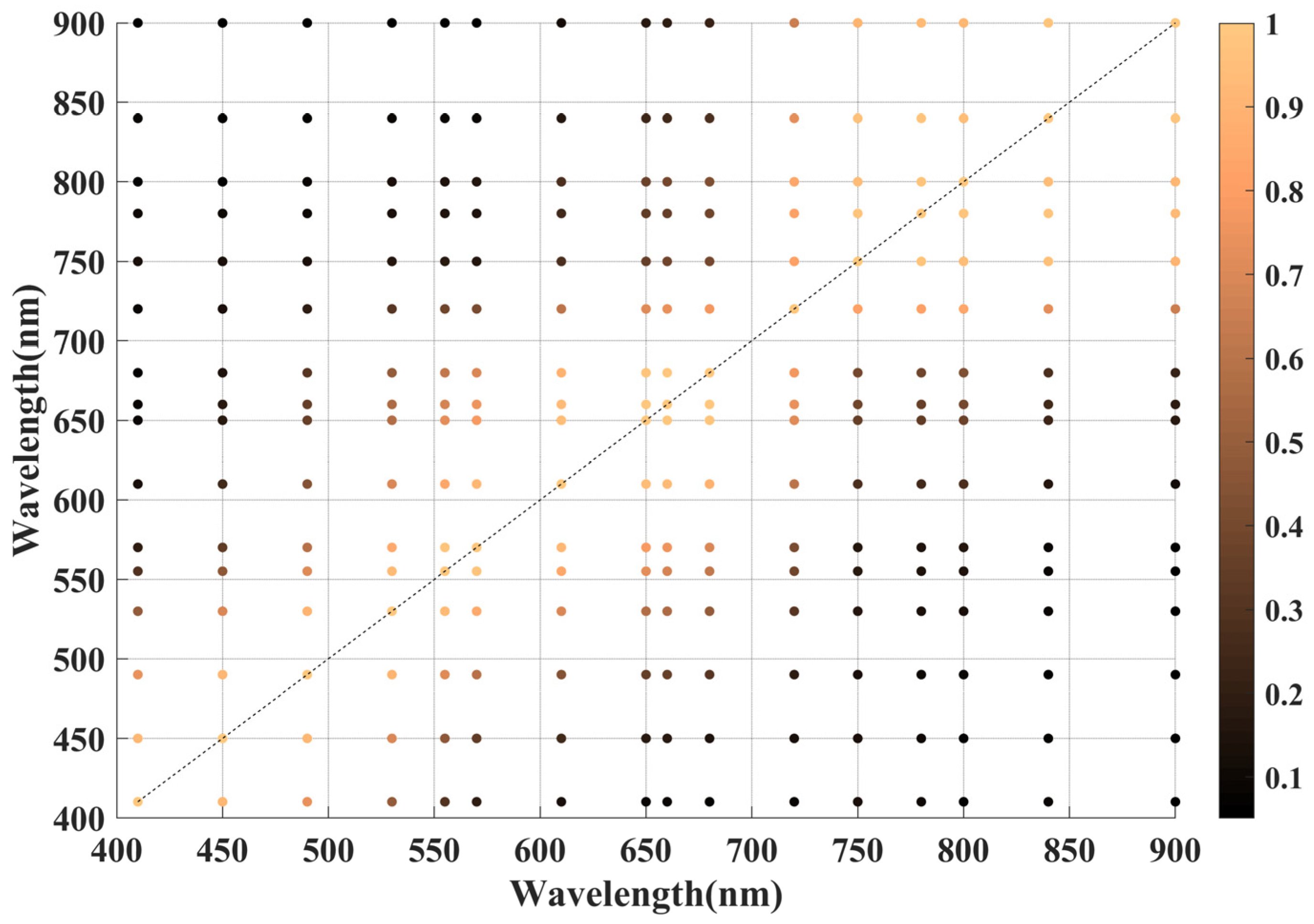
The determination coefficient R² between the reflectance data corresponding to each two-band combination for the CM16 band set are shown in Figure 12.

The combinations of the two spectral bands that cannot appear at the same time are shown in the

Table 7. Twenty groups of two-band combinations with high correlation.

No.	Wavelength of Band 1	Wavelength of Band 2	R2
1	410	450	0.92
2	450	490	0.92
3	530	555	0.94
4	555	570	0.98
5	570	610	0.91
6	610	650	0.95
7	610	660	0.93
8	650	660	1.00
9	650	680	0.98
10	660	680	0.99
11	750	780	0.98
12	750	840	0.96
13	750	800	0.94
14	750	900	0.90
15	780	800	0.98
16	780	840	0.98
17	780	900	0.93
18	800	840	0.95
19	800	900	0.91
20	840	900	0.97

, with a total of 20 groups.

The maximum number of spectral bands included in a spectral band combination and the number of different spectral band combinations with different numbers of bands were calculated, as shown in the

Table 8. Twenty groups of two-band combinations with high correlation.

Number of Bands	Number of All Combinations	Number of Combinations of This Method	Reduction Proportion
1	16	16	0%
2	120	100	16.67%
3	560	311	44.46%
4	1820	509	72.03%
5	4368	428	90.20%
6	8008	170	97.88%
7	11,440	25	99.78%
8	12,870	0	100.00%
total	39,202	1559	96.02%

. The reduction proportion refers to the decrease in computational load enabled by the proposed approach. Without this approach, it would be necessary to exhaustively enumerate and evaluate all possible band combinations, which scales exponentially with the number of bands. However, by intelligently pruning away invalid and redundant band combinations before evaluation, our method retains only 3.98% of the complete set of combinations. Thus, the discarded 96.02% of combinations that do not need to be explicitly evaluated lead to the stated reduction in computation. In summary, these percentages quantify the improvement in computational efficiency gained by avoiding brute-force evaluation of all combinations through the selective analysis proposed in this work. For instance, for combinations with seven bands, the number for the enumeration method will be 11,440. However, with the help of the proposed method described in this paper, the number of combinations that meet the requirements is only 25, which means only 0.2% computational load remained and 99.78% of the computational load was reduced.

As can be seen from the table, the maximum number of spectral bands included in a spectral band combination is 7. Compared with the enumeration method, the method proposed in this paper can reduce the calculation of characteristic spectral band combinations containing only 1–8 bands by 96.02%. Considering that combinations containing 9–16 bands do not need to be calculated, the total calculation can be reduced by 96.02%.

4.2. Result of the Empirical Method with 1, 2, and 3 Bands

Table 9. Optimal performance evaluation of various empirical regression models for different water quality parameters.

Parameters	Calculated Reflectance	$\overline{{\mathit{R}}^2}$	RMSE	MAPE	${\mathit{\lambda }}_1$/nm	${\mathit{\lambda }}_2$/nm	${\mathit{\lambda }}_3$/nm	Band Set
DO	$R_1$	0.015	2.653	25.35%	780			CM16
	$R_2^{BR}$	0.305	2.183	19.75%	610	650		CM16
	$R_2^{NDSI}$	0.309	2.178	19.75%	610	650		CM16
	$R_3^{TBI}$	0.288	2.163	19.65%	610	650	680	CM16
	$R_3^{ETBI}$	0.063	2.482	23.26%	530	555	570	CM16
	$R_3^{BH}$	0.270	2.192	19.23%	610	650	720	CM16
CODMn	$R_1$	0.052	1.358	25.45%	717			Mic
	$R_2^{BR}$	0.065	1.321	24.41%	530	610		CM16
	$R_2^{NDSI}$	0.080	1.311	23.99%	450	720		CM16\MS600\AQ600
	$R_3^{TBI}$	0.090	1.276	24.11%	530	555	580	CM16
	$R_3^{ETBI}$	−0.025	1.355	24.36%	490	680	800	CM16
	$R_3^{BH}$	0.067	1.292	23.61%	490	800	900	CM16
NH3-N	$R_1$	−0.006	0.319	74.29%	610			CM16
	$R_2^{BR}$	−0.029	0.317	74.20%	490	610		CM16
	$R_2^{NDSI}$	−0.035	0.318	74.45%	490	610		CM16
	$R_3^{TBI}$	−0.068	0.316	74.65%	490	610	900	CM16
	$R_3^{ETBI}$	−0.085	0.318	73.10%	490	610	650	CM16
	$R_3^{BH}$	−0.046	0.313	70.54%	750	780	900	CM16
TP	$R_1$	0.105	0.081	49.50%	720			CM16\MS600\AQ600
	$R_2^{BR}$	0.088	0.080	47.57%	490	720		CM16
	$R_2^{NDSI}$	0.087	0.080	47.65%	530	720		CM16
	$R_3^{TBI}$	0.035	0.080	48.71%	530	720	800	CM16
	$R_3^{ETBI}$	−0.023	0.083	50.27%	530	650	800	CM16
	$R_3^{BH}$	0.010	0.081	48.26%	555	660	680	CM16
TN	$R_1$	0.052	1.698	53.51%	717			Mic
	$R_2^{BR}$	0.076	1.642	51.44%	530	610		CM16
	$R_2^{NDSI}$	0.077	1.642	51.36%	530	610		CM16
	$R_3^{TBI}$	0.041	1.638	51.62%	530	610	750	CM16
	$R_3^{ETBI}$	−0.030	1.698	52.30%	475	668	717	Mic
	$R_3^{BH}$	0.047	1.633	51.97%	555	610	680	CM16
EC	$R_1$	0.060	149.764	22.74%	900			CM16
	$R_2^{BR}$	0.087	144.655	20.75%	450	730		DJ4
	$R_2^{NDSI}$	0.101	143.559	20.47%	450	730		DJ4
	$R_3^{TBI}$	0.038	145.329	21.37%	450	780	800	CM16
	$R_3^{ETBI}$	−0.067	153.069	22.57%	490	660	800	CM16
	$R_3^{BH}$	−0.008	148.832	21.61%	490	780	840	CM16
TUB	$R_1$	0.072	55.462	55.27%	680			CM16
	$R_2^{BR}$	0.153	51.931	50.10%	555	610		CM16
	$R_2^{NDSI}$	0.167	51.490	48.94%	530	680		CM16
	$R_3^{TBI}$	0.126	51.624	49.42%	555	610	660	CM16
	$R_3^{ETBI}$	−0.011	55.532	54.01%	530	650	800	CM16
	$R_3^{BH}$	0.208	49.170	45.84%	570	720	840	CM16

shows the $\overline{R^2}$, RMSE, and mean absolute percentage error (MAPE) [33] for the linear fitting results of the measured water quality parameters and the calculated reflectance for the one-, two-, and three-band empirical model methods, together with the center wavelengths of the bands corresponding to the model.

The empirical model parameters corresponding to each water quality parameter in the table with the best performance are shown in bold in Table 9. Taking $\overline{R^2}$ as the evaluation index, the accuracy of the optimal performance model $R_2^{NDSI}$ for DO is the highest among the different water quality parameters, with R² reaching 0.309 and MAPE 19.65%.

This is a three-band model, and the corresponding center wavelengths of the bands are 610, 650, and 680 nm, respectively. This band is combined from the band set CM16. The second is the optimal performance model $R_3^{BH}$ for TUB, which is a three-band model. The corresponding center wavelengths of the bands are 570, 720, and 840 nm, respectively, which are from the band set CM16. Its $\overline{R^2}$ reaches 0.208, but its MAPE is only 45.84%, which has a large relative error. The next were TP, EC, COD_Mn, and TN, with $\overline{R^2}$ of 0.105, 0.101, 0.90, and 0.077, respectively. It is worth noting that although the four $\overline{R^2}$ are similar, the MAPE for COD_Mn and EC is between 20% and 25%, while the MAPE for TP and TN is between 47% and 52%. NH3-N had the worst performance with $\overline{R^2}$; less than 0 and its optimal performance model was $R_1$ with MAPE reaching 74.29%. It worth noting that the center wavelengths of the corresponding bands of EC are 450 and 730 nm, respectively, which are from the band set DJ4.

For different empirical models and among the seven water quality parameters, there are two best performance models with three bands, which are $R_3^{TBI}$ and $R_3^{BH}$, respectively. There are three best performance models with three bands, among which $R_2^{BR}$ accounts for one and $\overline{R^2}$ accounts for two. There are two best performance models with one band. Most of the bands corresponding to the optimal performance model are from CM16, with the exception of the EC model, which is from the DJ4 band set.

In summary, among the band sets of different products, the fitting result of CM16 bands is the best, indicating that, generally, the more bands that can be selected, the better the fitting result. It shows that the empirical models with different band combinations cannot effectively determine the characteristic spectral bands for each water quality parameter, so it is necessary to use the ANN method to carry out the fitting inversion between the calculated reflectance of different band combinations with different band number and each water quality parameter, so as to determine and select the characteristic spectral bands for each water quality parameter.

4.3. Result of the ANN Method

Figure 13 depicts the performance results for the different ANN regression models, employing $\overline{R^2}$ as the evaluation index.

Figure 13 illustrates that the ANN method shows substantially better performance than the empirical method for the regression models of various water quality parameters. Among the optimal ANN regression models for different water quality parameters, the NH3-N model has the poorest performance, as measured by $\overline{R^2}$ of 0.41; nevertheless, this still exceeds the top empirical model (for DO) with an $\overline{R^2}$ of 0.309. The optimal model was for COD_Mn with an $\overline{R^2}$ of 0.68, followed by TUB, TP, TN, EC, DO, and NH3-N. The $\overline{R^2}$ values for the optimal TUB and TP ANN models all exceeded 0.6; the $\overline{R^2}$ for the optimal TN ANN model was 0.58, which is a single-band model; and the $\overline{R^2}$ values for all the optimal EC, DO, and NH3-N ANN models were in the range from 0.4 to 0.5. With the exception of TN, the optimal ANN models for the other water quality parameters were all three-band models, whereas the TN ANN model had one band.

For the various band sets, all bands corresponding to the optimal performance ANN models belonged to the CM16 band set. The ANN models for COD_Mn, NH3-N, TP, and TUB in the CM16 band set evidenced obvious advantages, with minimum R² differences greater than 0.1 compared to the other band sets. The $\overline{R^2}$ differences were all less than 0.1 between the ANN models for DO, TN, and EC in the CM16 band set compared to other band sets. Nevertheless, compared to other band sets, CM16 still demonstrated considerable dominance over other band sets, owing to the ample spectral band options it provides. The existing multispectral lens products are suitable for agriculture and forestry and have large errors in the inversion measurement of water quality parameters.

For ANN models with different band numbers, most models showed performance that increased with more bands except TN for band set CM16. It is necessary to study the performance of different band number models to determine the optimal number of bands for different water quality parameters.

Figure 14 illustrates the performance of ANN models of water quality parameters with varying numbers of spectral bands. As evidenced in Figure 14, all ANN models of water quality parameters exhibit a consistent pattern in which model accuracy, as measured by $\overline{R^2}$, initially increases with additional bands but subsequently decreases with the exception of TN models. For the ANN regression model of DO and NH3-N, $\overline{R^2}$ values increased monotonically from one to four bands and then decreased monotonically from four to seven bands. For the ANN regression model of CODMn, TP, EC, and NH3-N, $\overline{R^2}$ limbed monotonically from one to three bands but declined monotonically thereafter from three to seven bands. Counterintuitively, the model for TN manifests the greatest performance with one band. Overall, the $\overline{R^2}$ value of the models decreased as the number of bands increased. However, the four-band model and seven-band model had higher $\overline{R^2}$ values than the three-band model and six-band model, respectively.

In summary, despite the increasing availability of information with additional spectral bands, model performance does not improve indefinitely. For most water quality parameters, model efficacy reaches an apex with either three or four bands, beyond which superfluous information degrades predictive accuracy. The anomalous case of TN highlights the idiosyncrasies that can emerge in complex models. It can be extrapolated that a paucity of information precludes achieving optimal model accuracy due to insufficient critical data. Additionally, redundant information introduces random noise into the data, thereby undermining accuracy.

Therefore, there exist an optimal number of characteristic spectral bands for different water quality parameters. The optimal number of bands for DO and NH3-N is four, the optimal number of bands for COD_Mn, TP, EC, and TUB is three, and the optimal number of bands for TN is one, because the ANN models with these optimal numbers of bands demonstrated the best performance among the various models.

Figure 15 shows the performance and spectral band information for the optimal ANN models of seven water quality parameters. It can be seen that the ANN model for COD_Mn has the best performance among the water quality parameters, with an $\overline{R^2}$ of 0.68 and a MAPE of 14.02%. Though the ANN models for TUB and TP have relatively high $\overline{R^2}$ values of 0.67 and 0.61, respectively, their MAPE values of 36.19% and 28.09% are not low. The $\overline{R^2}$ values of EC and DO ANN regression models are 0.49 and 0.43, respectively, which do not show the advantage among water quality parameters; their MAPE values remain at low levels ranging from 16% to 18%. As with the results of the empirical method and the ANN method with other band sets, the performance of the NH3-N ANN model was the worst, with the lowest $\overline{R^2}$ of 0.54 and the highest MAPE of 65.85%.

Furthermore, Figure 15 shows that the characteristic spectral band combinations for COD_Mn and TP were the same, namely 410, 490, and 840 nm, which belonged to the set of DO characteristic spectral bands. The DO characteristic spectral bands differed from these two indices only in having an additional 720 nm band. The characteristic spectral bands for EC were 410, 570, and 720 nm, with the 410 and 720 nm bands overlapping with DO and the 570 nm band overlapping with NH3-N. The characteristic spectral bands for NH3-N were 490, 570, 680, and 840 nm, with the 490 n and 840 nm bands overlapping with DO, COD_Mn, and TP. The characteristic spectral band for TN was a single band with a center wavelength of 610 nm, and the characteristic spectral bands for TUB were 530, 660, and 780 nm. The biggest difference from the characteristic spectral bands of them between those of other water quality parameters was that there were no overlapping bands.

5. Discussion

This study also explored the relationship between characteristic spectral bands in the model as the number of bands increased, that is, whether the highly correlated bands in the model with fewer bands would also appear in the model with the best performance with more bands. However, the results did not show that the bands in the model with fewer bands would also appear in the model with the best performance of more bands. Therefore, this content was not discussed in detail.

This paper suggests that the spectral bands with wavelengths of 410, 490, 570, 680, 720, and 840 nm should be used if the researcher needs to customize a six-band multispectral camera to monitor the water quality parameters of DO, COD_Mn, NH3-N, TP, and EC and effectively ensure the inversion accuracy of COD_Mn, DO, and EC. The inversion accuracy of TN and TUB cannot be ensured. However, due to the common situation that TN exceeds the standard in general water bodies and that TUB is not used to classify water quality, the lack of accurate inversion of TN and TUB will not affect the water quality assessment. If there are other requirements, i.e., the water quality parameters in the research interest of the investigator, the optimal combination of six spectral bands can be determined according to the actual requirements, so as to achieve the optimal inversion result of all these water quality parameters.

The dataset in this paper was obtained from all of the NSWAMS of Suzhou, Shanghai, Jiaxing, Huzhou, and Wuxi in the Changjiang Delta region, covering the data of December 2020, January, November, December 2021, and March and August 2022. The data are diverse and can represent the characteristics of different time periods, and the model is suitable for the inversion of water quality parameters in this region. However, due to the good water quality and low degree of pollution, the dataset used for the training model has fewer class V and inferior class V water quality samples. The performance of the models in water quality inversion and classification is not good. At the same time, the applicability and universality of the model are directly related to the sample dataset during the model training. Therefore, with the progress of this research, the universality of the model can be effectively expanded by adding more regions and more periods of datasets to the model training. In addition, due to different target water quality parameters and different selected bands, there will certainly be different cameras with different spectral band combinations for different purposes, and the bands to be customized should be determined according to the actual needs.

6. Conclusions

This study discussed the determination of the optimal characteristic spectral bands for different water quality parameters with a proposed novel approach, which is based on the correlation between reflectance of different bands and regression modeling with the ANN method. Using fused ZY1-02D hyperspectral images and water quality data from December 2020 to August 2021 around Taihu Lake, the proposed approach was tested. The result showed that it can effectively reduce the computation by 96.02% and quickly find the characteristic bands to improve the modeling efficiency. Comparing different band sets of multispectral cameras, the CM16 band set with 16 bands leads to the best performance, suggesting that more spectral options enable better modeling results. Compared to typical empirical methods, the ANN model shows significant advantages in estimating various water quality parameters. Each parameter has an optimal number of characteristic bands, with model accuracy first increasing and then decreasing as more bands are added, except for TN.

The proposed approach and modeling method provide a new approach for effective spectral characteristic bands and precise estimation of water quality parameters from hyperspectral images. They lay a theoretical foundation for customized multispectral cameras and UAV platforms for water quality monitoring. This study provides a reference for follow-up research to customize multispectral lenses and develop UAV remote sensing techniques for water quality monitoring. The proposed characteristic band approach and modeling method can be extended to other hyperspectral remote sensing studies to address high data dimensionality and improve modeling efficiency.

References

1. Jay, S.; Guillaume, M. A Novel Maximum Likelihood Based Method for Mapping Depth and Water Quality from Hyperspectral Remote-Sensing Data. Remote Sens. Environ. 2014, 147, 121–132. [Google Scholar] [CrossRef]
2. Dall’Olmo, G.; Gitelson, A.A.; Rundquist, D.C. Towards a Unified Approach for Remote Estimation of Chlorophyll-a in Both Terrestrial Vegetation and Turbid Productive Waters. Geophys. Res. Lett. 2003, 30, 1938. [Google Scholar] [CrossRef]
3. Duan, H.; Ma, R.; Loiselle, S.A.; Shen, Q.; Yin, H.; Zhang, Y. Optical Characterization of Black Water Blooms in Eutrophic Waters. Sci. Total Environ. 2014, 482–483, 174–183. [Google Scholar] [CrossRef]
4. Wernand, M.R.; Hommersom, A.; Van Der Woerd, H.J. MERIS-Based Ocean Colour Classification with the Discrete Forel–Ule Scale. Ocean Sci. 2013, 9, 477–487. [Google Scholar] [CrossRef]
5. Terentev, A.; Dolzhenko, V.; Fedotov, A.; Eremenko, D. Current State of Hyperspectral Remote Sensing for Early Plant Disease Detection: A Review. Sensors 2022, 22, 757. [Google Scholar] [CrossRef]
6. Cao, Q.; Yu, G.; Qiao, Z. Application and Recent Progress of Inland Water Monitoring Using Remote Sensing Techniques. Environ. Monit. Assess. 2023, 195, 125. [Google Scholar] [CrossRef] [PubMed]
7. Vakili, T.; Amanollahi, J. Determination of Optically Inactive Water Quality Variables Using Landsat 8 Data: A Case Study in Geshlagh Reservoir Affected by Agricultural Land Use. J. Clean. Prod. 2020, 247, 119134. [Google Scholar] [CrossRef]
8. Wang, S.; Garcia, M.; Bauer-Gottwein, P.; Jakobsen, J.; Zarco-Tejada, P.J.; Bandini, F.; Paz, V.S.; Ibrom, A. High Spatial Resolution Monitoring Land Surface Energy, Water and CO2 Fluxes from an Unmanned Aerial System. Remote Sens. Environ. 2019, 229, 14–31. [Google Scholar] [CrossRef]
9. Cao, Y.; Ye, Y.; Zhao, H.; Jiang, Y.; Wang, H.; Shang, Y.; Wang, J. Remote Sensing of Water Quality Based on HJ-1A HSI Imagery with Modified Discrete Binary Particle Swarm Optimization-Partial Least Squares (MDBPSO-PLS) in Inland Waters: A Case in Weishan Lake. Ecol. Inform. 2018, 44, 21–32. [Google Scholar] [CrossRef]
10. Wang, Y.; Li, S.; Lin, Y.; Wang, M. Lightweight Deep Neural Network Method for Water Body Extraction from High-Resolution Remote Sensing Images with Multisensors. Sensors 2021, 21, 7397. [Google Scholar] [CrossRef]
11. Yang, Z.; Gong, C.; Ji, T.; Hu, Y.; Li, L. Water Quality Retrieval from ZY1-02D Hyperspectral Imagery in Urban Water Bodies and Comparison with Sentinel-2. Remote Sens. 2022, 14, 5029. [Google Scholar] [CrossRef]
12. Sudduth, K.A.; Jang, G.-S.; Lerch, R.N.; Sadler, E.J. Long-Term Agroecosystem Research in the Central Mississippi River Basin: Hyperspectral Remote Sensing of Reservoir Water Quality. J. Environ. Qual. 2015, 44, 71–83. [Google Scholar] [CrossRef]
13. Kudela, R.M.; Palacios, S.L.; Austerberry, D.C.; Accorsi, E.K.; Guild, L.S.; Torres-Perez, J. Application of Hyperspectral Remote Sensing to Cyanobacterial Blooms in Inland Waters. Remote Sens. Environ. 2015, 167, 196–205. [Google Scholar] [CrossRef]
14. Hestir, E.L.; Brando, V.E.; Bresciani, M.; Giardino, C.; Matta, E.; Villa, P.; Dekker, A.G. Measuring Freshwater Aquatic Ecosystems: The Need for a Hyperspectral Global Mapping Satellite Mission. Remote Sens. Environ. 2015, 167, 181–195. [Google Scholar] [CrossRef]
15. Lei, S.; Wu, D.; Li, Y.; Wang, Q.; Huang, C.; Liu, G.; Zheng, Z.; Du, C.; Mu, M.; Xu, J.; et al. Remote Sensing Monitoring of the Suspended Particle Size in Hongze Lake Based on GF-1 Data. Int. J. Remote Sens. 2019, 40, 3179–3203. [Google Scholar] [CrossRef]
16. Li, Y.; Zhang, Y.; Shi, K.; Zhu, G.; Zhou, Y.; Zhang, Y.; Guo, Y. Monitoring Spatiotemporal Variations in Nutrients in a Large Drinking Water Reservoir and Their Relationships with Hydrological and Meteorological Conditions Based on Landsat 8 Imagery. Sci. Total Environ. 2017, 599–600, 1705–1717. [Google Scholar] [CrossRef] [PubMed]
17. Lim, J.; Choi, M. Assessment of Water Quality Based on Landsat 8 Operational Land Imager Associated with Human Activities in Korea. Environ. Monit. Assess. 2015, 187, 384. [Google Scholar] [CrossRef] [PubMed]
18. Gholizadeh, M.; Melesse, A.; Reddi, L. A Comprehensive Review on Water Quality Parameters Estimation Using Remote Sensing Techniques. Sensors 2016, 16, 1298. [Google Scholar] [CrossRef]
19. Gordon, H.R.; Brown, O.B.; Jacobs, M.M. Computed Relationships between the Inherent and Apparent Optical Properties of a Flat Homogeneous Ocean. Appl. Opt. 1975, 14, 417–427. [Google Scholar] [CrossRef] [PubMed]
20. Dekker, A.G.; Vos, R.J.; Peters, S.W.M. Analytical Algorithms for Lake Water TSM Estimation for Retrospective Analyses of TM and SPOT Sensor Data. Int. J. Remote Sens. 2002, 23, 15–35. [Google Scholar] [CrossRef]
21. Gordon, H.R.; Morel, A.Y. Remote Assessment of Ocean Color for Interpretation of Satellite Visible Imagery: A Review; Lecture Notes on Coastal and Estuarine Studies; American Geophysical Union: Washington, DC, USA, 1983; Volume 4, ISBN 978-0-387-90923-3. [Google Scholar]
22. Gitelson, A.A.; Schalles, J.F.; Hladik, C.M. Remote Chlorophyll-a Retrieval in Turbid, Productive Estuaries: Chesapeake Bay Case Study. Remote Sens. Environ. 2007, 109, 464–472. [Google Scholar] [CrossRef]
23. Le, C.; Hu, C.; Cannizzaro, J.; English, D.; Muller-Karger, F.; Lee, Z. Evaluation of Chlorophyll-a Remote Sensing Algorithms for an Optically Complex Estuary. Remote Sens. Environ. 2013, 129, 75–89. [Google Scholar] [CrossRef]
24. Lei, S.; Xu, J.; Li, Y.; Li, L.; Lyu, H.; Liu, G.; Chen, Y.; Lu, C.; Tian, C.; Jiao, W. A Semi-Analytical Algorithm for Deriving the Particle Size Distribution Slope of Turbid Inland Water Based on OLCI Data: A Case Study in Lake Hongze. Environ. Pollut. 2021, 270, 116288. [Google Scholar] [CrossRef] [PubMed]
25. Zeng, S.; Lei, S.; Li, Y.; Lyu, H.; Dong, X.; Li, J.; Cai, X. Remote Monitoring of Total Dissolved Phosphorus in Eutrophic Lake Taihu Based on a Novel Algorithm: Implications for Contributing Factors and Lake Management. Environ. Pollut. 2022, 296, 118740. [Google Scholar] [CrossRef] [PubMed]
26. Zhang, D.; Zhang, L.; Sun, X.; Gao, Y.; Lan, Z.; Wang, Y.; Zhai, H.; Li, J.; Wang, W.; Chen, M.; et al. A New Method for Calculating Water Quality Parameters by Integrating Space–Ground Hyperspectral Data and Spectral-In Situ Assay Data. Remote Sens. 2022, 14, 3652. [Google Scholar] [CrossRef]
27. Doerffer, R.; Schiller, H. The MERIS Case 2 Water Algorithm. Int. J. Remote Sens. 2007, 28, 517–535. [Google Scholar] [CrossRef]
28. Pahlevan, N.; Smith, B.; Schalles, J.; Binding, C.; Cao, Z.; Ma, R.; Alikas, K.; Kangro, K.; Gurlin, D.; Hà, N.; et al. Seamless Retrievals of Chlorophyll-a from Sentinel-2 (MSI) and Sentinel-3 (OLCI) in Inland and Coastal Waters: A Machine-Learning Approach. Remote Sens. Environ. 2020, 240, 111604. [Google Scholar] [CrossRef]
29. Zhang, D.; Zeng, S.; He, W. Selection and Quantification of Best Water Quality Indicators Using UAV-Mounted Hyperspectral Data: A Case Focusing on a Local River Network in Suzhou City, China. Sustainability 2022, 14, 16226. [Google Scholar] [CrossRef]
30. Yin, F.; Wu, M.; Liu, L.; Zhu, Y.; Feng, J.; Yin, C.; Yin, C. Predicting the abundance of copper in soil using reflectance spectroscopy and GF5 hyperspectral imagery. Int. J. Appl. Earth Obs. 2021, 102, 102420. [Google Scholar] [CrossRef]
31. Niroumand-Jadidi, M.; Bovolo, F.; Bruzzone, L. Water Quality Retrieval from PRISMA Hyperspectral Images: First Experience in a Turbid Lake and Comparison with Sentinel-2. Remote Sens. 2020, 12, 3984. [Google Scholar] [CrossRef]
32. Li, L.; Gu, M.; Gong, C.; Hu, Y.; Wang, X.; Yang, Z.; He, Z. An Advanced Remote Sensing Retrieval Method for Urban Non-Optically Active Water Quality Parameters: An Example from Shanghai. Sci. Total Environ. 2023, 880, 163389. [Google Scholar] [CrossRef]
33. Liu, H.; Yu, T.; Hu, B.; Hou, X.; Zhang, Z.; Liu, X.; Liu, J.; Wang, X.; Zhong, J.; Tan, Z.; et al. UAV-Borne Hyperspectral Imaging Remote Sensing System Based on Acousto-Optic Tunable Filter for Water Quality Monitoring. Remote Sens. 2021, 13, 4069. [Google Scholar] [CrossRef]
34. Bi, S. Remote Sensing of Algal Column Integrated Biomass for Inland Waters Based on Soft Classification; College of Geographical Science: Nanjing, China, 2021. [Google Scholar]
35. Liu, Y.; Li, J.; Xiao, C.; Zhang, F.; Wang, S. Inland Water Chlorophyll-a Retrieval Based on ZY-1 02D Satellite Hyperspectral Observations. Natl. Remote Sens. Bull. 2022, 26, 168–178. [Google Scholar] [CrossRef]
36. Moses, W.J.; Gitelson, A.A.; Berdnikov, S.; Povazhnyy, V. Satellite Estimation of Chlorophyll-a Concentration Using the Red and NIR Bands of MERIS—The Azov Sea Case Study. IEEE Geosci. Remote Sens. Lett. 2009, 6, 845–849. [Google Scholar] [CrossRef]
37. Mishra, S.; Mishra, D.R. Normalized Difference Chlorophyll Index: A Novel Model for Remote Estimation of Chlorophyll-a Concentration in Turbid Productive Waters. Remote Sens. Environ. 2012, 117, 394–406. [Google Scholar] [CrossRef]
38. Gitelson, A.A.; Dall’Olmo, G.; Moses, W.; Rundquist, D.C.; Barrow, T.; Fisher, T.R.; Gurlin, D.; Holz, J. A Simple Semi-Analytical Model for Remote Estimation of Chlorophyll-a in Turbid Waters: Validation. Remote Sens. Environ. 2008, 112, 3582–3593. [Google Scholar] [CrossRef]
39. Yang, W.; Matsushita, B.; Chen, J.; Fukushima, T.; Ma, R. An Enhanced Three-Band Index for Estimating Chlorophyll-a in Turbid Case-II Waters: Case Studies of Lake Kasumigaura, Japan, and Lake Dianchi, China. IEEE Geosci. Remote Sens. Lett. 2010, 7, 655–659. [Google Scholar] [CrossRef]
40. Wynne, T.T.; Stumpf, R.P.; Briggs, T.O. Comparing MODIS and MERIS Spectral Shapes for Cyanobacterial Bloom Detection. Int. J. Remote Sens. 2013, 34, 6668–6678. [Google Scholar] [CrossRef]
41. Najwa Mohd Rizal, N.; Hayder, G.; Mnzool, M.; Elnaim, B.M.E.; Mohammed, A.O.Y.; Khayyat, M.M. Comparison between Regression Models, Support Vector Machine (SVM), and Artificial Neural Network (ANN) in River Water Quality Prediction. Processes 2022, 10, 1652. [Google Scholar] [CrossRef]
42. Piepho, H. An Adjusted Coefficient of Determination for Generalized Linear Mixed Models in One Go. Biom. J. 2023, 65, 2200290. [Google Scholar] [CrossRef]
Figure 1. Overall technical flowchart for this work.
Remotesensing 15 05578 g001
Figure 2. Research area of water quality and satellite data.
Remotesensing 15 05578 g002
Figure 3. Preprocessing flow of hyperspectral data from satellite ZY1-02D.
Remotesensing 15 05578 g003
Figure 4. One of the ZY1-02D satellite image products.
Remotesensing 15 05578 g004
Figure 5. Principle of heterogeneous data matching between hyperspectral satellite data and water quality parameters records.
Remotesensing 15 05578 g005
Figure 6. Detailed steps in heterogeneous data matching between hyperspectral satellite data and water quality parameters records.
Remotesensing 15 05578 g006
Figure 7. Classifications distribution of water quality parameters: (a) original 188 records; (b) 90 records after analysis and screening.
Remotesensing 15 05578 g007
Figure 8. Remote sensing hyperspectral spectral curve with the wavelength from 390 to 900 nm.
Remotesensing 15 05578 g008
Figure 9. Spectral curves for multispectral data with 26 spectral bands.
Remotesensing 15 05578 g009
Figure 10. Approach for determining the characteristic spectral bands of water quality parameters.
Remotesensing 15 05578 g010
Figure 11. ANN model construction and training method.
Remotesensing 15 05578 g011
Figure 12. Cloud image of reflectance correlation of 16 spectral bands.
Remotesensing 15 05578 g012
Figure 13. R 2 ¯ for the ANN regression model using different band sets with one, two, and three bands for DO (a), CODMn (b), NH3-N (c), TP (d), TN (e), EC (f), and TUB (g).
Remotesensing 15 05578 g013aRemotesensing 15 05578 g013b
Figure 14. R 2 ¯ for ANN models of different water quality parameters with different numbers of spectral bands.
Remotesensing 15 05578 g014
Figure 15. Performance validation and spectral band information for the optimal ANN model of DO (a), CODMn (b), NH3-N (c), TP (d), TN (e), EC (f), and TUB (g).
Remotesensing 15 05578 g015