Article

Spatial and Spectral Translation of Landsat 8 to Sentinel-2 Using Conditional Generative Adversarial Networks

1
School of Geography, Development, and Environment, The University of Arizona, Tucson, AZ 85721, USA
2
Department of Geography, The Ohio State University, Columbus, OH 43210, USA
*
Author to whom correspondence should be addressed.
These authors contributed equally to this work.
Remote Sens. 2023, 15(23), 5502; https://doi.org/10.3390/rs15235502
Submission received: 21 October 2023 / Revised: 21 November 2023 / Accepted: 23 November 2023 / Published: 25 November 2023
(This article belongs to the Special Issue Remote Sensing Data Fusion and Applications)

Abstract

:
Satellite sensors like Landsat 8 OLI (L8) and Sentinel-2 MSI (S2) provide valuable multispectral Earth observations that differ in spatial resolution and spectral bands, limiting synergistic use. L8 has a 30 m resolution and a lower revisit frequency, while S2 offers up to a 10 m resolution and more spectral bands, such as red edge bands. Translating observations from L8 to S2 can increase data availability by combining their images to leverage the unique strengths of each product. In this study, a conditional generative adversarial network (CGAN) is developed to perform sensor-specific domain translation focused on green, near-infrared (NIR), and red edge bands. The models were trained on the pairs of co-located L8-S2 imagery from multiple locations. The CGAN aims to downscale 30 m L8 bands to 10 m S2-like green and 20 m S2-like NIR and red edge bands. Two translation methodologies are employed—direct single-step translation from L8 to S2 and indirect multistep translation. The direct approach involves predicting the S2-like bands in a single step from L8 bands. The multistep approach uses two steps—the initial model predicts the corresponding S2-like band that is available in L8, and then the final model predicts the unavailable S2-like red edge bands from the S2-like band predicted in the first step. Quantitative evaluation reveals that both approaches result in lower spectral distortion and higher spatial correlation compared to native L8 bands. Qualitative analysis supports the superior fidelity and robustness achieved through multistep translation. By translating L8 bands to higher spatial and spectral S2-like imagery, this work increases data availability for improved earth monitoring. The results validate CGANs for cross-sensor domain adaptation and provide a reusable computational framework for satellite image translation.

1. Introduction

Satellite sensors capture multispectral observations of the Earth’s surface at different spatial resolutions. Typically, there is a trade-off between spatial resolution and acquisition revisit time (temporal resolution) for a single sensor [1]. Higher spatial resolution sensors often have a narrower swath width and a lower revisit frequency. Furthermore, cloud cover is a major issue for optical imagery that further reduces image availability. To obtain more frequent cloud-free observations, satellite constellations can be formed using multiple satellites with similar sensors [2]. For example, the Sentinel-2 (S2) constellation launched by the European Space Agency (ESA) consists of Sentinel-2A MSI (2015) and Sentinel-2B MSI (2017), each with 13 spectral bands at spatial resolutions of 10 m, 20 m, and 60 m. The S2 constellation improves the temporal acquisition frequency from 10 days to 5 days. Commercial satellite imagery, obtained by Planet through a constellation of approximately 24 operational satellites, provides the capability to capture near-daily images with a resolution of 3 m. In addition to satellite constellations, virtual constellations of different satellite sensors, i.e., combining existing satellite observations of similar characteristics, provide a viable way to mitigate the limitations of a single sensor [1,3,4,5,6].
Several studies have investigated the benefits of the combined use of Landsat 8 OLI (L8) with S2 [7,8,9,10,11]. Hao et al. [12] took advantage of the greater number of cloud-free pixels available of combined L8 and S2 products to improve crop intensity mapping. Tulbure et al. [13] leveraged the denser frequency of combined L8 and S2 to capture temporally dynamic ephemeral floods in drylands. In addition to enhancing temporal frequency, another added value of combining L8 and S2 is enhanced spectral information. S2 contains three red-edge spectral bands between the wavelengths of red and near-infrared that are not available in L8. The red-edge spectral bands increase land-use and land-cover mapping accuracy [14] and are beneficial for measuring leaf area index [15], estimating chlorophyll content [16], improving the mapping accuracy of wetlands [17], and land-use and land-cover change [18].
Despite the spatial and spectral similarity between L8 and S2, there are differences in spatial resolution and spectral bands between the two sensors that lead to uncertainty when directly combined without adequate pre-processing. To harmonize the two satellite sensors, Claverie et al. [19] developed Harmonized Landsat and Sentinel-2 (HLS) products by combining seven common L8 and S2 spectral bands to generate 30 m spatially co-registered Landsat-like bands at 5-day intervals. In the HLS products, L8 and S2 are spatially harmonized by resampling the S2 data into 30 m grids that overlap with L8 and spectrally harmonized through spectral bandpass adjustment using 150 globally distributed hyperspectral Hyperion images. Since the release of HLS products, they have been used in various remote sensing applications because of their increased data availability [12,20,21,22]. In addition, several methods have been developed to improve harmonization between L8 and S2 [23,24,25,26,27]. Shang and Zhu [24] proposed an improved algorithm to harmonize the two datasets through a time series-based reflectance adjustment (TRA) approach to minimize the difference in surface reflectance. However, both HLS and TRA generate images at 30 m that do not take advantage of the higher spatial resolution S2 imagery. Hence, to incorporate the higher spatial details provided by S2, Shao et al. [23] and Pham and Bui [27] used a deep learning-based fusion method to learn the non-linear relationship and generate images at a higher spatial resolution of 10 m. Shao et al. [23] used a convolutional neural network (CNN) to predict 10 m L8 images with the help of S2 data during training, while Pham and Bui [27] used a Generative Adversarial Network (GAN). However, both studies excluded the S2 red edge bands in their analysis. Conversely, Scheffler et al. [25] simulated L8-like and S2-like images from airborne hyperspectral images and then applied regression and machine learning algorithms to predict S2-like red edge bands from L8 at 30 m, which shares the same limitations as HLS and TRA regarding spatial details. Only one harmonization study targeted 10 m resolution and included red edge bands [26]. Isa et al. [26] trained a super-resolution CNN model to predict the S2-like red edge bands at 10 m from L8. However, CNNs are limited by their user-defined loss function and do not learn from real data, unlike GANs. Recently, Chen et al. [28] developed a feature-level data fusion framework using a GAN to reconstruct 10 m Sentinel-2-like imagery from 30 m historical Landsat archives. Their GAN-based super-resolution method demonstrated effective reconstruction of synthetic Landsat data to Sentinel-2 observations, thus suggesting potential for improving both spatial and spectral resolutions of harmonized products between L8 and S2. It is evident that existing harmonization methods and products have incentivized and improved the synergistic use of L8 and S2, but more research is needed to enhance both the spatial and spectral resolutions of harmonized products between L8 and S2.
Translating L8 to S2-like images can be defined as a domain transfer problem, where the two sensors, L8 and S2 (the two domains), capture the same land surface area. Image translation algorithms can transfer domain-specific information from one domain to another, for example, Goodfellow et al. [29] proposed a deep learning-based framework for similar domain adaptation tasks using adversarial networks. Subsequently, their GAN framework has been effectively used for several image-processing tasks, such as image super-resolution [30], registration [31], classification [32], and translation [33]. An example of the efficacy of GANs in enhancing spatial resolution is provided by Kong et al. [34], who used a dual GAN model to super-resolve historical Landsat imagery for long-term vegetation monitoring. Isola et al. [33] developed a conditional GAN (CGAN) for translating images across multiple domains, for example, translating satellite imagery to maps. Their network learned the representations between the two domains to predict an image from the desired distribution (e.g., maps) given an image from the source distribution (e.g., satellite imagery). Following the advancements in generative modeling using GANs, remote sensing researchers have addressed the issue of satellite data availability by translating multi-sensor images. Recent work has explored the generation of synthetic bands for existing satellites as a way to synchronize multispectral data across different data products, utilizing a combination of variational autoencoders and generative adversarial networks [35]. Merkle et al. [36] explored the potential of GANs for optical and SAR image matching. Ao et al. [37] translated publicly available low-resolution Sentinel-1 data to commercial high-resolution TerraSAR-X using a dialectical generative adversarial network (DiGAN). Bermudez et al. [38] synthesized optical and SAR imagery for cloud removal using GAN and Fuentes Reyes et al. [39] generated alternative representations of SAR by synthesizing SAR and optical imagery to improve visual interpretability. Akiva et al. [40] synthesized PlanetScope-like SWIR bands from S2 to improve flood segmentation using GANs. Recently, Sedona et al. [41] employed a multispectral generative adversarial network to achieve high performance in harmonizing dense time series of Landsat-8 and Sentinel-2 images. Their approach not only produced higher-quality images but also demonstrated superior crop-type mapping accuracy in comparison to existing methods. In fact, Pham and Bui [27] applied GANs to enhance L8 spatial resolution to match S2. Therefore, the success of GANs in translating satellite images across domains provides an ideal opportunity for translating L8 to S2, particularly for predicting the additional red-edge bands of S2 from L8.
In this paper, we define this task of predicting S2-like images from L8 images as an image translation task where we train a conditional GAN to translate L8 spectral bands to S2-like spectral bands. In addition to predicting the common spectral bands between L8 and S2, we generate S2-like red edge bands from L8 images that are not present in the L8 product. More specifically, we investigate the performance of CGANs in predicting five S2-like spectral bands—green, red edge 1, red edge 2, red edge 3, and narrow near-infrared (NIR) from two spectral bands of L8—green and NIR. In addition to evaluating the benefits of CGANs, we evaluated two approaches for predicting S2-like red edge bands from L8—direct and multistep. The multistep approach divides the task into two parts to reduce per-model complexity. First, we predict the S2 spectral band from the equivalent L8 spectral band before attempting to predict the red edge bands that are not available in L8. In the case of the direct approach, the CGANs are trained to predict the red edge bands directly from the most correlated L8 bands.

2. Materials and Methods

2.1. Landsat 8 and Sentinel-2 Scenes

We acquired spatially coincident relatively cloud-free level 2 atmospherically corrected surface reflectance L8 and S2 scenes from 2019. L8 was downloaded from USGS Earth Explorer and S2 was downloaded from Sentinel Hub. L8 scenes have a larger spatial footprint compared to S2; therefore, multiple S2 scenes (with the same acquisition date) were mosaicked to build some of the L8-S2 scene pairs. The path/row of L8 scenes and the corresponding tile IDs S2 scenes are provided in Table 1. In total, 11 S2 scenes and 5 L8 scenes were processed to create 5 L8-S2 scene pairs. Since same-day acquisitions of L8 and S2 are not very common for a given location, we allowed a maximum gap of 3 days between the acquisitions. Consequently, this temporal gap resulted in some land surface changes. There were occurrences of cloud cover and cloud shadow in the image pairs. However, due to the differences in image acquisition times of the sensors, these pixels were present only in one of the L8 and S2 pairs. Figure 1 shows two examples: (a) cloud-free and (b) cloud-covered examples from the training datasets.

2.2. Training Dataset Preparation

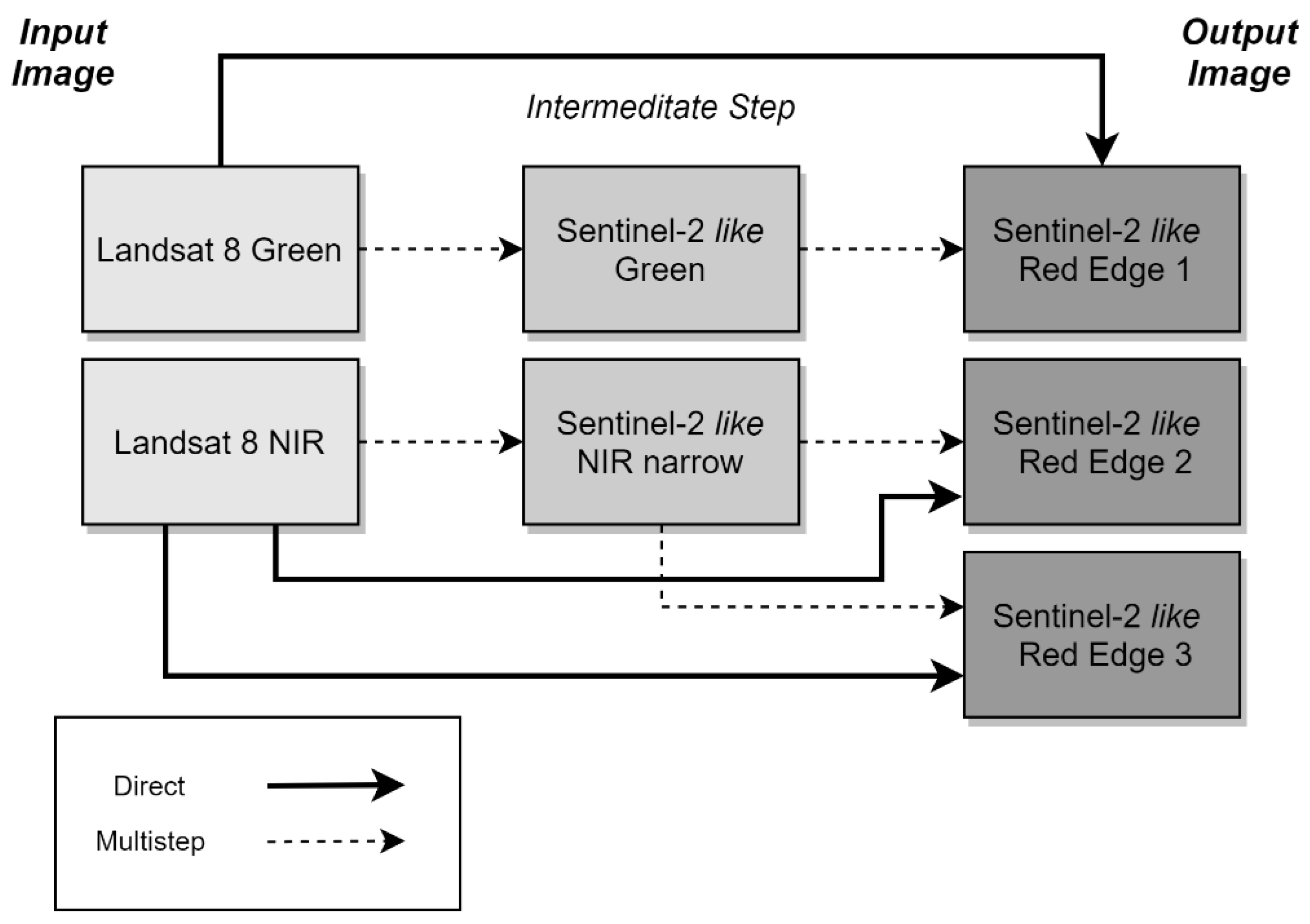
In this study, we selected the green and NIR spectral bands from L8, along with the green, narrow NIR, and red edge bands (RE1, RE2, RE3) from S2. Table 2 shows the details of the wavelength ranges and spatial resolutions of these selected bands. As described in the methodology in Section 2 (Figure 2), we generated five separate training datasets for the translation of each S2 band from its corresponding L8 band. While the trend in the literature involves employing a deep learning model to learn multiple bands in one single task, we argue that this approach increases the task’s complexity. In contrast, training separate models for each spectral band allows each model to focus on learning the representations solely between two specific bands.
Each L8 band was resampled to match the spatial resolution of its corresponding S2 band using nearest neighbor interpolation; for instance, L8 green at 30 m was resampled to S2 green at 10 m. This technique was chosen to ensure that the original surface reflectance values remained unchanged, as opposed to using bilinear or bicubic. Given that the L8 green band also serves to predict S2 RE1, we matched their spatial resolutions during the data pre-processing steps by resampling 20 m S2 RE1 to 10 m.
The L8 and S2 imagery were then spatially aligned through clipping them. However, we encountered spatial registration inconsistencies between L8 and S2, a phenomenon also observed by Storey et al. [42] and attributable to spatial resolution disparities. For example, a 30 m L8 pixel may encapsulate up to nine 10 m S2 pixels, leading to unavoidable misregistration issues as emphasized by Jiang et al. [43]. To reduce this, we employed a phase correlation technique [44] to reduce this error. Keeping S2 constant, we slid the L8 image in each direction to find the coordinates with the highest correlation.
After reducing misregistration errors and spatially aligning each pair, we extracted image patches of dimensions 256 × 256 from both the L8 and S2 datasets. The choice of a 256 × 256 patch size was a trade-off between capturing sufficient spatial context for the model and the computational constraints imposed by our GPU capabilities. Opting for larger image patches would necessitate reducing the batch size, a modification that could increase the risk of model overfitting. Due to the resampling of L8 green and S2 RE1 to a 10 m spatial resolution (refer to Section 2, Figure 2), the dataset comprised 7552 image pairs for these particular bands. Similarly, the dataset for the 20 m S2 NIR, S2 RE2, S2 RE3, and the resampled L8 NIR (from 30 m to 20 m) contained 3291 training images each. For the purposes of model validation and testing, we randomly partitioned 5% of the total data into separate validation and test sets. These subsets consisted of 375 images for the 10 m dataset and 80 image patches for the 20 m dataset.

2.3. Methodology

L8 has several spectral bands whose wavelength overlaps with S2 spectral bands (see Table 2), and these bands exhibit a strong correlation across L8 and S2 [7]. One of our research aims is to understand the relationships between these common spectral bands across the two sensors. While the task of translating common bands—such as L8 green to S2 green or L8 NIR to S2 NIR—may appear straightforward, the complexity arises from the disparity in wavelength ranges covered by the spectral bands across L8 and S2. Indeed, translating S2 RE bands, which are absent in L8, introduces additional complexity. To address this challenge, Scheffler et al. [25] employed hyperspectral data to simulate Landsat and Sentinel-2 bands; conversely, GAN techniques have been successfully applied in translating across more disparate domains like optical to SAR [45].
We, therefore, opted to predict Sentinel-2-like RE bands by translating the L8 band exhibiting the highest correlation with each of the S2 RE bands. In ref. [31], the authors determined the correlation coefficients between the S2 bands across multiple scenes and discovered that the S2 green band had the highest correlation with S2 RE1; similarly, S2 NIR narrow exhibited the highest correlation with S2 RE2 and RE3. We developed two distinct strategies. The first involves directly predicting the S2-like RE bands from the L8 band that most closely correlates with them, as studied by Mandanici and Bitelli [7]. This is referred to as our direct approach.
Our multistep approach introduces an intermediary translation phase: initially, we translate the L8 band to its corresponding S2 band—for instance, L8 green to S2-like green. Subsequently, we derive the S2-like RE band from the translated S2-like band, as evidenced in Figure 2. The multistep approach operates under two assumptions: first, deconstructing the complex translation task into simpler sub-tasks can enhance model performance; and second, the incorporation of additional reference imagery via an additional step could improve both model accuracy and robustness.

2.4. Conditional Generative Adversarial Network

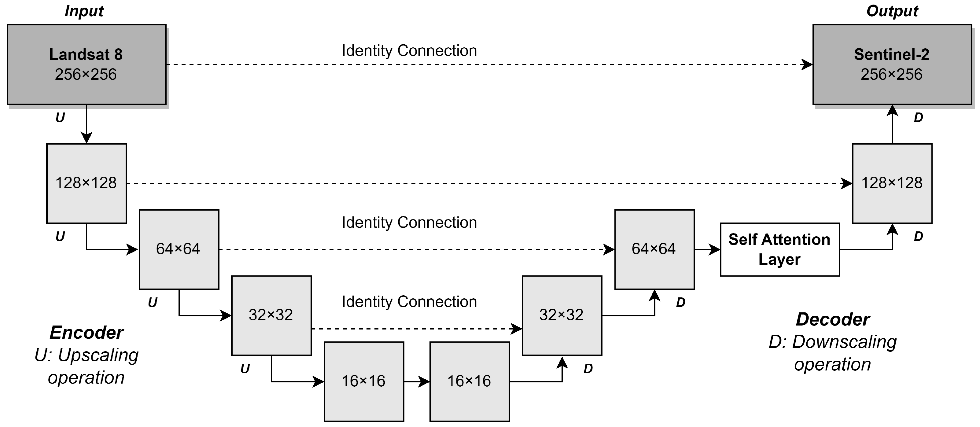
The deep learning architecture is based on the conditional generative adversarial network (CGAN) proposed by [33]. The task of the generator is to generate samples belonging to the target distribution (e.g., an S2-like spectral band) from the source distribution (L8 spectral bands), while the task of the discriminator is to help improve the transformative ability of the generator by learning to differentiate between S2-like bands (estimated from L8 bands) and original S2 bands. Figure 3 shows our generator architecture, which consists of two networks—an encoder and a decoder network. The encoder and the decoder networks progressively upscale and downscale the images, respectively, to learn the representations between the image pairs at multiple scales. Spatial information is preserved through identity connections at each scale before upscaling/downscaling operations. We implemented U-Net based architecture [46] with a ResNet-34 as our encoder and added a self-attention layer [47] similar to [48] to preserve the global dependencies during the reconstruction of the target image. The loss function of the generator was mean average error or L1.
The discriminator is based on the architecture PatchGAN, as defined by Isola et al. [33]. This architecture divides the input image from the generator into smaller patches. The discriminator receives S2 images from two distributions—original S2 images and the translated S2-like images by the generator one at a time. The network then assesses each patch to determine if it is more similar to the original S2 distribution or the S2-like distribution generated by the generator. The loss function of the discriminator, which is the mean average error or L1, learns to differentiate between the two sets, helping the network to classify the image generated by the generator into these two categories.
The objectives of the generator and the discriminator networks are adversarial. For example, the generator aims to generate S2-like images that are ideally indistinguishable from original S2 images, while the discriminator learns to effectively distinguish the generated S2-like images from the original S2 images, participating in a minimax game [29]. The objective function V(G, D) in Equation (1) defines the performance metrics for the generator (G) and discriminator (D) within a GAN framework. The D maximizes V(G, D) through accurate classification of real versus synthetic images. The G minimizes V(G, D), creating images from a latent distribution z that mimics the real data distribution x from Sentinel-2 (S2). The D evaluates the input images to assign probabilities that identify their source (original S2 or S2-like from G). Equilibrium is attained when the D probability assessment for both image types converges to 0.5, indicating the G’s effectiveness in generating from the real S2 image distribution.
V ( G , D ) = E x P Sentinel - 2 ( x ) [ log D ( x ) ] + E z P Landsat 8 ( z ) [ log ( 1 D ( G ( z ) ) ) ]
CGANs can be difficult to train; therefore, we followed DeOldify’s [49] NoGAN training process to improve network training stability. Following this strategy, we pre-trained our G for 10 epochs separately and then we trained our D for 10 epochs on the generated images by the pre-trained generator. Next, we trained both G and D for 80 epochs switching between the networks with multiple learning rates. We used a loss threshold for our discriminator to make sure that it does not improve significantly relative to the generator. If the discriminator becomes significantly better than the generator, the overall training accuracy of our CGAN will not improve any further. Figure 4 shows an overview of our network setup.

2.5. Method Comparison and Evaluation

We expect our CGAN to learn the representation between the source (L8) and the target set (S2) to predict S2-like images spatially and spectrally close to the original S2. Therefore, we evaluated the translations by CGAN against the original S2 spectral bands. We evaluated the performances of our CGAN both quantitatively and qualitatively. We used metrics that are widely used in the field of remote sensing to quantitatively evaluate satellite images, including Erreur Relative Globale Adimensionnelle de Synthèse (ERGAS; [50]), spectral angle mapper (SAM; [51]), spatial correlation coefficient (SCC; [52]), peak signal-to-noise ratio (PSNR [53]), root mean squared error (RMSE), and Universal Quality Image Index (UQI; [54]). ERGAS and SAM are useful for assessing spectral differences, whereas SCC and PSNR evaluate spatial reconstruction. RMSE and UQI provide a more holistic assessment of the quality of translations. We visually observed the differences between the predicted and the target images for qualitative evaluation. Table 3 describes each metric and its ideal score. In addition to the results from the architectures, we compared the results with the original Landsat 8 images as a baseline to measure the actual improvements by these methods.

3. Results

We evaluate the performance of CGANs towards translating S2-like green and NIR bands using the corresponding L8 green and NIR bands. Next, we evaluate two approaches: direct and multistep, towards translating S2-like RE1, RE2, and RE3 bands from L8 green and NIR bands.

3.1. Translating S2-like Green and NIR Spectral Bands from L8

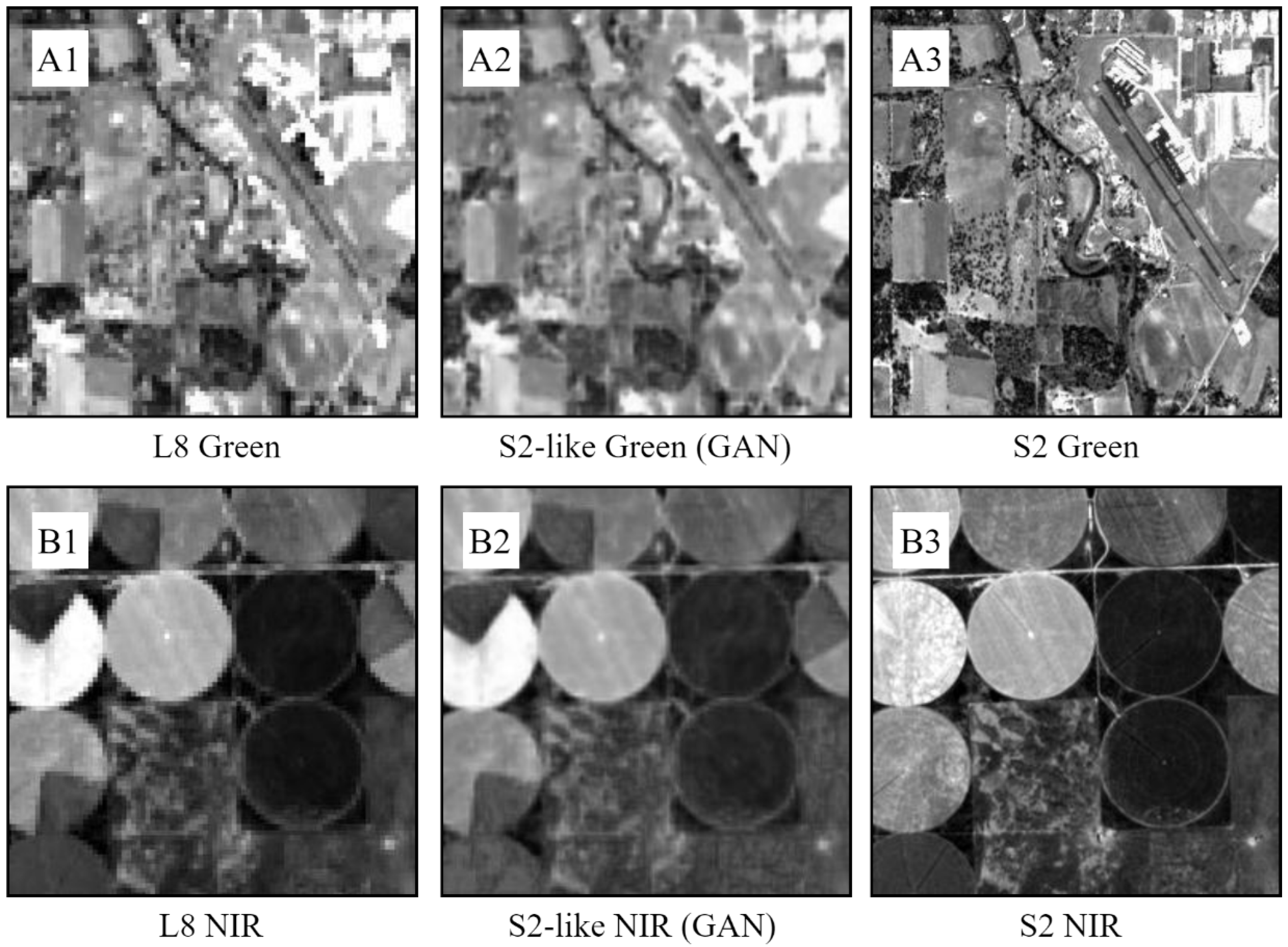
Figure 5 shows the S2-like green and NIR images translated by CGAN. Our CGAN downscaled L8 green (30 m) to S2-like green (10 m) at a scale factor of 3. The network increased the effective spatial resolution of the L8 green images which is noticeable through the clear and less pixelated edges of the river and roads in the translated image (Figure 5(A2)). Further, CGAN translated 30 m L8 NIR images to 20 m S2-like NIR narrow images by downscaling the images at a scale factor of 1.5. Even at a low scale factor, the translations by the network are sharper than the original L8 NIR images, as observed from the edges of the agricultural patches. According to the quantitative evaluation (Table 4), CGAN minimized spectral and spatial differences between the L8 and S2 images across all metrics. Most improvements can be observed through the increase in the spatial correlation coefficient (SCC), signifying that CGAN was able to reconstruct the finer spatial features of the higher-resolution S2 images accurately. Figure 6 shows layer-stacked images of the L8 and S2 images along with the translations. Each image in the figure (see Figure 6) is layer-stacked with NIR, green, and green (repeated), respectively. To layer stack the images, the 20 m S2-like NIR images were downscaled to match the 10 m spatial resolution of the S2 green band using bilinear interpolation. We observe (Figure 6) that the network increased spatial resolution of the L8 images which is most noticeable through the sharper road networks and building boundaries. Additionally, the network was able to maintain spectral fidelity as we did not observe any spectral distortion between the predicted and the target images.

3.2. Translating S2-like RE1, RE2, and RE3 Bands from L8

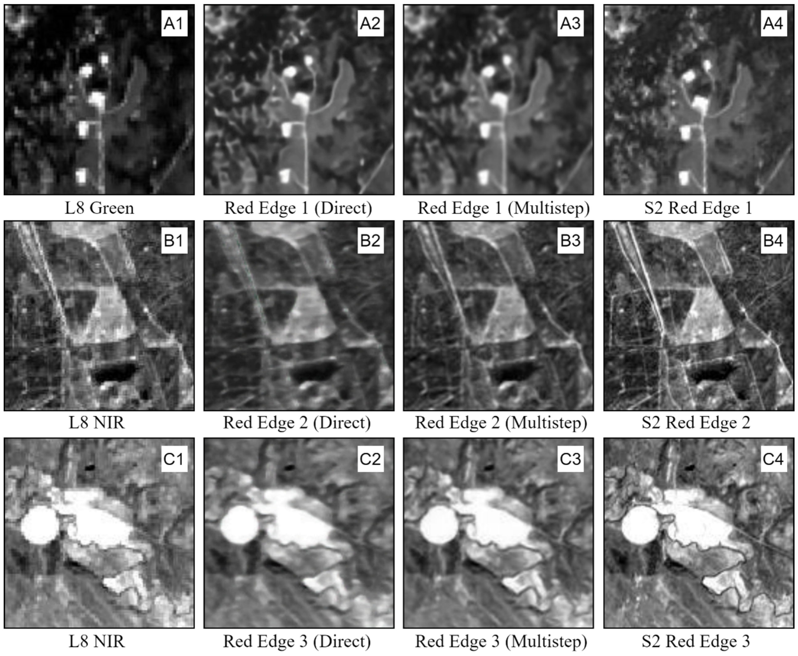
Figure 7 shows the S2-like RE1, RE2, and RE3 translations by CGAN using two different approaches—direct and multistep. The objective for both of these approaches was to downscale the 30 m L8 green bands to 20 m S2-like RE1 bands at a scale factor of 1.5. However, to accommodate the multistep approach, all images are resampled to 10 m to match the resolution of the S2 green band. From the results, we observe a noticeable improvement in the spatial resolution from the original L8 from both direct and multistep approaches. We observe that both strategies were effective at translating S2-like RE1 bands (Figure 7(A2)) that are spectrally more similar to the target S2 RE1 image compared to the L8 green image. Since the target S2 RE1 images were resampled to a higher resolution of 10 m compared to its original resolution of 20 m, the CGANs in the direct approach were able to reconstruct the spatial features at a finer spatial resolution. We observe that the direct approach produced visually better results compared to the multistep approach. Interestingly, resampling the image to a higher spatial resolution also allowed the direct CGAN to produce sharper images than the 20 m S2 RE1. In contrast, the multistep approach produced images that are spatially and texturally similar to the original 20 m S2 RE1. This is due to the additional step in which the CGAN first translates the L8 green to S2-like green and then translates the S2-like green image to the target S2-like RE1. The additional step allows the network to learn the spatial representations between the input and the target images more accurately, hence producing images that are qualitatively and quantitatively more similar to the target 20 m S2 RE1 images. This feature of the multistep approach is observed in its better quantitative performance compared to the direct approach (Table 5).
Similarly, the two approaches were used to translate 20 m S2-like RE2 and RE3 images from 30 m L8 NIR. From Figure 7 we observe that both approaches improved the spatial resolution of the predicted S2-like RE2 and RE3 images from L8 NIR. Unlike the case for predicting the S2-like RE1 bands, predicting the RE2 and RE3 bands did not require further resampling steps for spatial resolution matching. S2 NIR, which is required as an intermediate step for the multistep method, and the target RE2 and RE3 images have the same spatial resolution at 20 m. Therefore, it is not surprising that the multistep method took advantage of an additional learning step and produced sharper images compared to the direct method (Figure 7(B2,B3,C2,C3)). From the quantitative evaluation results reported in Table 5, we observe that the performance of both direct and multistep approaches is comparable as they minimize the gap between L8 NIR and the S2-like RE2 and RE3 bands. We layer stacked S2-like RE1, RE2, and RE3 bands translated by both the approaches (Figure 8), to compare spatial and spectral reconstruction. Each RGB image is layer-stacked with RE3, RE1, and RE2 in that order, except the L8 scene. The L8 scene in Figure 8A is layer-stacked with the spectral bands with which each RE band was predicted, i.e., NIR (for predicting SR3), green (for predicting SR1), and NIR (for predicting SR2). Overall, we observe that both direct (Figure 8B) and multistep (Figure 8C) approaches reduced the spectral gap between the L8 and the target S2 images significantly. However, discernible differences can be observed in the spectral reconstruction performances of the two approaches. Images produced by the direct approach exhibit artificial noise, while those generated through the multistep method appear visibly cleaner. The additional learning step in the multistep method allows for a more stable translation performance.

4. Discussion

4.1. CGAN Performance towards Predicting S2-like Spectral Bands

CGANs were effective in translating S2-like spectral bands from L8 bands. They reduced the spectral difference between the spectral bands available in both sensors (i.e., green and NIR). CGANs also spatially enhanced the original L8 images to match the target S2 spectral bands. Of the two approaches used to predict the additional S2-like RE bands from L8, the multistep method produced qualitatively better and more consistent results than the direct approach. Breaking the more complex task of predicting S2-like bands from L8 into two smaller tasks—translating the corresponding S2-like band from the L8 band, and then translating the S2-like band from the previous step to the target S2-like red edge band, produces better quality images. However, the direct approach performed quantitatively better. Multistep CGANs benefited from the intermediate step since there is a stronger relationship among the bands of each step (L8 NIR to S2 NIR and S2 NIR to S2 red edge) compared to the relationship between L8 NIR and the S2 RE bands. CGANs learned the finer spatial features from S2 bands, and this was most evident for multistep methods since the network could learn from two sets of data (intermediate and target S2 images). This feature of CGANs should be exploited for generating images at a higher spatial resolution than the original images by incorporating additional finer resolution imagery if possible. Therefore, CGANs can effectively learn the spatial as well as spectral representations between the two satellite products and do not simply reduce the per-pixel average error between the input and target images.

4.2. Improving CGAN Performance

The performance of CGANs can be improved with the help of a more efficient training dataset design. For example, using L8 and S2 scene pairs acquired on the same date can increase network accuracy. Our scene pairs (input L8 and target S2) had some temporal gaps (see Table 1), which could introduce some uncertainty due to the possibility of land surface changes occurring between each image acquisition by L8 and S2. In terms of spatial generalizability, this method can be applied to any region provided there exist observations from both sensors for that region within an acceptable time frame. CGAN’s performance could be increased for the region of interest by fine-tuning the model on additional L8-S2 scene pairs acquired from that specific region and over multiple timestamps. Furthermore, instead of using a single L8 spectral band to predict each S2-like RE band, training our CGAN on multiple L8 spectral bands may allow the network to predict each RE band more accurately. To predict the RE bands, we used the spectral bands with the highest correlation with them following the study by Mandanici and Bitelli [7]. However, the strength of correlation typically varies across land use/land cover classes and was not addressed in this study. Therefore, measuring the spatial and spectral similarity between L8 and S2 spectral bands over different land use/land cover classes could give a better idea of which L8 spectral bands should be used for predicting the desired S2 bands.

4.3. Advantages of CGANs over CNNs

Even though this paper mainly focused on CGANs, we also investigated other deep learning architectures, such as convolutional networks (CNNs) for our image translation task. CNNs have been widely used for image-processing tasks [55], more specifically, Shao et al. [23] used CNN for downscaling L8 imagery to S2-like spatial resolution, Isa et al. [26] trained a super-resolution CNN model to predict the S2-like red edge bands at 10 m from L8. However, CGANs have an advantage over CNNs for image regression tasks, including image translation due to their adaptable loss function. To demonstrate the benefits of generative adversarial training, we compared CGANs with CNNs. We trained the CNN on the training dataset for the same task (translating S2-like spectral bands from L8). Even though CNNs could marginally outperform CGANs during training, they would likely underperform during testing. It was found that CNNs were not robust to outliers. When CNNs were tasked to predict from out-of-the-distribution “real world” training pairs that may be considered an outlier, for example, misregistered pairs of L8 and S2, the translations were less accurate than CGANs (Figure 9). This sensitivity to out-of-the-distribution training data reduces model stability. This suboptimal performance of CNNs is likely due to its predefined loss function, which primarily attempts to reduce the overall mean error between the input and target image pairs. CGANs, on the other hand, learn from the original distributions of both sets—L8 and S2, enough to differentiate between the two products. We encountered several suboptimal training pairs that had misregistration issues due to the pixel mismatch between the spatial resolutions of L8 and S2 (described in Section 2.2). CNN erroneously learned to produce blurry images for such samples, while CGAN-generated images are more likely to belong to real S2 imagery. Figure 9 demonstrates two cases of misregistered image pairs. We observe that the images predicted by CGANs appear sharper than the blurry images predicted by the CNNs. The results are consistent with the observations by Ledig et al. [30] with respect to the characteristics of these two network architectures. Since achieving spatial generalizability with any model is non-trivial, GANs would be a more reliable architecture for image-to-image translation tasks.

4.4. Limitations of CGANs

Although CGANs are effective for predicting S2 from L8 imagery, there are certain limitations that should be addressed. For example, CGANs have a more complex training process that requires significantly more time to train, around four-fold for each CNN. The performance of CGANs greatly depends on the quality of the dataset and the complexity of the task. CGANs require considerably more manual supervision during training since there is no specific objective function to minimize, unlike convolution networks that only look to reduce the loss function. Therefore, training CGANs typically requires running multiple experiments, which increases overall training time substantially. However, the NoGAN training methodology proposed by Antic [49] reduces some of the training uncertainty and helps stabilize this process. Despite these difficulties, CGANs are effective in image translation [30] and other image-processing tasks [56]. Although CGANs and other deep learning algorithms require large datasets and computational resources for training, access to publicly available satellite datasets [57] and computational resources reduces such issues.

4.5. Future Work

Future work will focus on improving the discriminator loss function, for example, Wasserstein loss [58] could be more effective in training the discriminator network since the feedback is more nuanced compared to the stricter class probabilities from the BCE loss. The training dataset for CGAN can be built based on the different biomes and seasons to capture the relationships between the two sensors for building a more spatially generalizable model. Similar to the harmonization task of L8 and S2, the CGAN model can also be used to harmonize L8, Landsat 7 ETM+ (L7), and Landsat 5 (L5). Generating L8-like data from L7 (launched in 1999) and L5 (launched in 1984) will allow us to take advantage of the entire Landsat archive, building upon the works of Savage et al. [59] and Vogeler et al. [60]. Reconstructed time series from combining these sensors could be used to analyze the leaf area index to further demonstrate the potential of the method. The CGAN model can be trained to translate S2 to predict higher spatial resolution PlanetScope-like spectral bands at 3 m, building on the work by Martins et al. [61]. Predicting near-daily PlanetScope-like imagery from Sentinel-2 would generate higher-quality publicly available data.

5. Conclusions

Our research contributes to the growing list of L8 and S2 harmonization methods developed for their synergistic use. Harmonized L8 and S2 satellite data are useful for reliable monitoring of natural resources such as vegetation and water, especially for applications that require more temporal data. In this paper, we propose a conditional generative adversarial network (CGAN) for predicting S2-like images from L8. Based on the results, we find that CGANs are effective in increasing the spatial resolution of the L8 spectral bands to match with the S2 bands. Secondly, CGANs can predict the three red edge bands available only in S2 from available L8 spectral bands, demonstrating its ability to increase the spectral resolution of a satellite product. Hence, CGANs can be used to translate L8 data for increasing the temporal resolution of the original S2 data product. Thirdly, CGANs generate S2-like imagery that is closer to the original S2 data compared to CNNs, making them more robust to outliers. This capability of CGANs highlights their benefit, despite the more complex training process they require. While our method was successful in translating Landsat 8 to S2, it can be used to translate satellite data products that have similar measurement principles and comparable spatial resolutions.

Author Contributions

Conceptualization, R.M. and D.L.; writing—original draft preparation, R.M.; writing—review and editing, D.L.; visualization, R.M.; supervision, D.L. All authors have read and agreed to the published version of the manuscript.

Funding

This research received no external funding.

Data Availability Statement

The data and code are presented in this study are available publicly at https://github.com/Rohit18/Landsat8-Sentinel2-Fusion (accessed on 20 October 2023).

Conflicts of Interest

The authors declare no conflict of interest.

References

  1. Wulder, M.A.; Hilker, T.; White, J.C.; Coops, N.C.; Masek, J.G.; Pflugmacher, D.; Crevier, Y. Virtual Constellations for Global Terrestrial Monitoring. Remote Sens. Environ. 2015, 170, 62–76. [Google Scholar] [CrossRef]
  2. Justice, C.O.; Townshend, J.R.G.; Vermote, E.F.; Masuoka, E.; Wolfe, R.E.; Saleous, N.; Morisette, J.T. An overview of MODIS Land data processing and product status. Remote Sens. Environ. 2002, 83, 3–15. [Google Scholar] [CrossRef]
  3. Zhu, X.; Helmer, E.H.; Gao, F.; Liu, D.; Chen, J.; Lefsky, M.A. A Flexible Spatiotemporal Method for Fusing Satellite Images with Different Resolutions. Remote Sens. Environ. 2016, 172, 165–177. [Google Scholar] [CrossRef]
  4. Li, J.; Roy, D.P. A global analysis of Sentinel-2A, Sentinel-2B and Landsat-8 data revisit intervals and implications for terrestrial monitoring. Remote Sens. 2017, 9, 902. [Google Scholar]
  5. Trishchenko, A.P. Clear-Sky Composites over Canada from Visible Infrared Imaging Radiometer Suite: Continuing MODIS Time Series into the Future. Can. J. Remote Sens. 2019, 45, 276–289. [Google Scholar] [CrossRef]
  6. Liang, J.; Liu, D. An Unsupervised Surface Water Un-Mixing Method Using Landsat and Modis Images for Rapid Inundation Observation. In Proceedings of the IGARSS 2019-2019 IEEE International Geoscience and Remote Sensing Symposium, Yokohama, Japan, 28 July–2 August 2019; pp. 9384–9387. [Google Scholar]
  7. Mandanici, E.; Bitelli, G. Preliminary Comparison of Sentinel-2 And Landsat 8 Imagery for A Combined Use. Remote Sens. 2016, 8, 1014. [Google Scholar]
  8. Chastain, R.; Housman, I.; Goldstein, J.; Finco, M.; Tenneson, K. Empirical Cross Sensor Comparison of Sentinel-2A And 2B MSI, Landsat-8 OLI, And Landsat-7 ETM+ Top of Atmosphere Spectral Characteristics over the Conterminous United States. Remote Sens. Environ. 2019, 221, 274–285. [Google Scholar] [CrossRef]
  9. Piedelobo, L.; Hernández-López, D.; Ballesteros, R.; Chakhar, A.; Del Pozo, S.; González-Aguilera, D.; Moreno, M.A. Scalable Pixel-Based Crop Classification Combining Sentinel-2 And Landsat-8 Data Time Series: Case Study of the Duero River Basin. Agric. Syst. 2019, 171, 36–50. [Google Scholar] [CrossRef]
  10. Zhang, Y.; Ling, F.; Wang, X.; Foody, G.M.; Boyd, D.S.; Li, X.; Atkinson, P.M. Tracking small-scale tropical forest disturbances: Fusing the Landsat and Sentinel-2 data record. Remote Sens. Environ. 2021, 261, 112470. [Google Scholar] [CrossRef]
  11. Silvero, N.E.Q.; Demattê, J.A.M.; Amorim, M.T.A.; Dos Santos, N.V.; Rizzo, R.; Safanelli, J.L.; Bonfatti, B.R. Soil Variability and Quantification Based on Sentinel-2 And Landsat-8 Bare Soil Images: A Comparison. Remote Sens. Environ. 2021, 252, 112117. [Google Scholar] [CrossRef]
  12. Hao, P.Y.; Tang, H.J.; Chen, Z.X.; Le, Y.U.; Wu, M.Q. High Resolution Crop Intensity Mapping Using Harmonized Landsat-8 and Sentinel-2 Data. J. Integr. Agric. 2019, 18, 2883–2897. [Google Scholar] [CrossRef]
  13. Tulbure, M.G.; Broich, M.; Perin, V.; Gaines, M.; Ju, J.; Stehman, S.V.; Betbeder-Matibet, L. Can we detect more ephemeral floods with higher density harmonized Landsat Sentinel 2 data compared to Landsat 8 alone? ISPRS J. Photogramm. Remote Sens. 2022, 185, 232–246. [Google Scholar] [CrossRef]
  14. Forkuor, G.; Dimobe, K.; Serme, I.; Tondoh, J.E. Landsat-8 Vs. Sentinel-2: Examining the Added Value of Sentinel-2’s Red-Edge Bands to Land-Use and Land-Cover Mapping in Burkina Faso. GISci. Remote Sens. 2018, 55, 331–354. [Google Scholar] [CrossRef]
  15. Dong, T.; Liu, J.; Shang, J.; Qian, B.; Ma, B.; Kovacs, J.M.; Shi, Y. Assessment Of Red-Edge Vegetation Indices for Crop Leaf Area Index Estimation. Remote Sens. Environ. 2019, 222, 133–143. [Google Scholar] [CrossRef]
  16. Delegido, J.; Verrelst, J.; Alonso, L.; Moreno, J. Evaluation Of Sentinel-2 Red-Edge Bands for Empirical Estimation of Green LAI And Chlorophyll Content. Sensors 2011, 11, 7063–7081. [Google Scholar] [CrossRef] [PubMed]
  17. Kaplan, G.; Avdan, U. Evaluating the Utilization of the Red Edge and Radar Bands from Sentinel Sensors for Wetland Classification. Catena 2019, 178, 109–119. [Google Scholar] [CrossRef]
  18. Chaves, E.D.M.; Picoli, C.A.M.; Sanches, D.I. Recent Applications of Landsat 8/OLI and Sentinel-2/MSI for Land Use and Land Cover Mapping: A Systematic Review. Remote Sens. 2020, 12, 3062. [Google Scholar] [CrossRef]
  19. Claverie, M.; Masek, J.G.; Ju, J.; Dungan, J.L. Harmonized Landsat-8 Sentinel-2 (HLS) Product User’s Guide; National Aeronautics and Space Administration (NASA): Washington, DC, USA, 2017. [Google Scholar]
  20. Mulverhill, C.; Coops, N.C.; Achim, A. Continuous monitoring and sub-annual change detection in high-latitude forests using Harmonized Landsat Sentinel-2 data. ISPRS J. Photogramm. Remote Sens. 2023, 197, 309–319. [Google Scholar] [CrossRef]
  21. Bolton, D.K.; Gray, J.M.; Melaas, E.K.; Moon, M.; Eklundh, L.; Friedl, M.A. Continental-scale land surface phenology from harmonized Landsat 8 and Sentinel-2 imagery. Remote Sens. Environ. 2020, 240, 111685. [Google Scholar] [CrossRef]
  22. Chen, N.; Tsendbazar, N.E.; Hamunyela, E.; Verbesselt, J.; Herold, M. Sub-annual tropical forest disturbance monitoring using harmonized Landsat and Sentinel-2 data. Int. J. Appl. Earth Obs. Geoinf. 2021, 102, 102386. [Google Scholar] [CrossRef]
  23. Shao, Z.; Cai, J.; Fu, P.; Hu, L.; Liu, T. Deep Learning-Based Fusion of Landsat-8 And Sentinel-2 Images for A Harmonized Surface Reflectance Product. Remote Sens. Environ. 2019, 235, 111425. [Google Scholar] [CrossRef]
  24. Shang, R.; Zhu, Z. Harmonizing Landsat 8 and Sentinel-2: A time-series-based reflectance adjustment approach. Remote Sens. Environ. 2019, 235, 111439. [Google Scholar] [CrossRef]
  25. Scheffler, D.; Frantz, D.; Segl, K. Spectral Harmonization and Red Edge Prediction of Landsat-8 To Sentinel-2 Using Land Cover Optimized Multivariate Regressors. Remote Sens. Environ. 2020, 241, 111723. [Google Scholar] [CrossRef]
  26. Isa, S.M.; Suharjito, S.; Kusuma, G.P.; Cenggoro, T.W. Supervised conversion from Landsat-8 images to Sentinel-2 images with deep learning. Eur. J. Remote Sens. 2021, 54, 182–208. [Google Scholar] [CrossRef]
  27. Pham, V.D.; Bui, Q.T. Spatial resolution enhancement method for Landsat imagery using a Generative Adversarial Network. Remote Sens. Lett. 2021, 12, 654–665. [Google Scholar] [CrossRef]
  28. Chen, B.; Li, J.; Jin, Y. Deep learning for feature-level data fusion: Higher resolution reconstruction of historical landsat archive. Remote Sens. 2021, 13, 167. [Google Scholar] [CrossRef]
  29. Goodfellow, I.J.; Pouget-Abadie, J.; Mirza, M.; Xu, B.; Warde-Farley, D.; Ozair, S.; Bengio, Y. Generative Adversarial Networks. arXiv 2014, arXiv:1406.2661. [Google Scholar] [CrossRef]
  30. Ledig, C.; Theis, L.; Huszár, F.; Caballero, J.; Cunningham, A.; Acosta, A.; Shi, W. Photo-Realistic Single Image Super-Resolution Using a Generative Adversarial Network. In Proceedings of the IEEE Conference on Computer Vision and Pattern Recognition, Honolulu, HI, USA, 21–26 July 2017; pp. 4681–4690. [Google Scholar]
  31. Quan, D.; Wang, S.; Liang, X.; Wang, R.; Fang, S.; Hou, B.; Jiao, L. Deep Generative Matching Network for Optical and SAR Image Registration. In Proceedings of the IGARSS 2018-2018 IEEE International Geoscience and Remote Sensing Symposium, Valencia, Spain, 22–27 July 2018; pp. 6215–6218. [Google Scholar]
  32. Zhu, L.; Chen, Y.; Ghamisi, P.; Benediktsson, J.A. Generative Adversarial Networks for Hyperspectral Image Classification. IEEE Trans. Geosci. Remote Sens. 2018, 56, 5046–5063. [Google Scholar] [CrossRef]
  33. Isola, P.; Zhu, J.Y.; Zhou, T.; Efros, A.A. Image-To-Image Translation with Conditional Adversarial Networks. In Proceedings of the IEEE Conference on Computer Vision and Pattern Recognition, Honolulu, HI, USA, 21–26 July 2017; pp. 1125–1134. [Google Scholar]
  34. Kong, J.; Ryu, Y.; Jeong, S.; Zhong, Z.; Choi, W.; Kim, J.; Houborg, R. Super resolution of historic Landsat imagery using a dual generative adversarial network (GAN) model with CubeSat constellation imagery for spatially enhanced long-term vegetation monitoring. ISPRS J. Photogramm. Remote Sens. 2023, 200, 1–23. [Google Scholar] [CrossRef]
  35. Vandal, T.J.; McDuff, D.; Wang, W.; Duffy, K.; Michaelis, A.; Nemani, R.R. Spectral synthesis for geostationary satellite-to-satellite translation. IEEE Trans. Geosci. Remote Sens. 2021, 60, 1–11. [Google Scholar] [CrossRef]
  36. Merkle, N.; Auer, S.; Müller, R.; Reinartz, P. Exploring The Potential of Conditional Adversarial Networks for Optical and SAR Image Matching. IEEE J. Sel. Top. Appl. Earth Obs. Remote Sens. 2018, 11, 1811–1820. [Google Scholar] [CrossRef]
  37. Ao, D.; Dumitru, C.O.; Schwarz, G.; Datcu, M. Dialectical GAN For SAR Image Translation: From Sentinel-1 To Terrasar-X. Remote Sens. 2018, 10, 1597. [Google Scholar] [CrossRef]
  38. Bermudez, J.D.; Happ, P.N.; Oliveira, D.A.B.; Feitosa, R.Q. SAR To Optical Image Synthesis for Cloud Removal with Generative Adversarial Networks. ISPRS Ann. Photogramm. Remote Sens. Spat. Inf. Sci. 2018, 4, 5–11. [Google Scholar] [CrossRef]
  39. Fuentes Reyes, M.; Auer, S.; Merkle, N.; Henry, C.; Schmitt, M. Sar-To-Optical Image Translation Based on Conditional Generative Adversarial Networks—Optimization, Opportunities and Limits. Remote Sens. 2019, 11, 2067. [Google Scholar] [CrossRef]
  40. Akiva, P.; Purri, M.; Dana, K.; Tellman, B.; Anderson, T. H2O-Net: Self-Supervised Flood Segmentation via Adversarial Domain Adaptation and Label Refinement. In Proceedings of the IEEE/CVF Winter Conference on Applications of Computer Vision, Virtual, 5 October 2021; pp. 111–122. [Google Scholar]
  41. Sedona, R.; Paris, C.; Cavallaro, G.; Bruzzone, L.; Riedel, M. A high-performance multispectral adaptation GAN for harmonizing dense time series of landsat-8 and sentinel-2 images. IEEE J. Sel. Top. Appl. Earth Obs. Remote Sens. 2021, 14, 10134–10146. [Google Scholar] [CrossRef]
  42. Storey, J.; Roy, D.P.; Masek, J.; Gascon, F.; Dwyer, J.; Choate, M. A Note on The Temporary Misregistration of Landsat-8 Operational Land Imager (OLI) And Sentinel-2 Multi Spectral Instrument (MSI) Imagery. Remote Sens. Environ. 2016, 186, 121–122. [Google Scholar] [CrossRef]
  43. Jiang, J.; Johansen, K.; Tu, Y.H.; McCabe, M.F. Multi-sensor and multi-platform consistency and interoperability between UAV, Planet CubeSat, Sentinel-2, and Landsat reflectance data. GISci. Remote Sens. 2022, 59, 936–958. [Google Scholar] [CrossRef]
  44. Ojansivu, V.; Heikkila, J. Image Registration Using Blur-Invariant Phase Correlation. IEEE Signal Process. Lett. 2007, 14, 449–452. [Google Scholar] [CrossRef]
  45. Zhao, Y.; Celik, T.; Liu, N.; Li, H.C. A Comparative Analysis of GAN-based Methods for SAR-to-optical Image Translation. IEEE Geosci. Remote Sens. Lett. 2022, 19, 1–5. [Google Scholar] [CrossRef]
  46. Ronneberger, O.; Fischer, P.; Brox, T. U-net: Convolutional networks for biomedical image segmentation. In Proceedings of the International Conference on Medical Image Computing and Computer-Assisted Intervention, Vancouver, BC, Canada, 8–12 October 2015; Springer: Cham, Switzerland, 2015; pp. 234–241. [Google Scholar]
  47. Zhang, H.; Goodfellow, I.; Metaxas, D.; Odena, A. Self-Attention Generative Adversarial Networks. In Proceedings of the International Conference on Machine Learning (PMLR), Long Beach, CA, USA, 9–15 June 2019; pp. 7354–7363. [Google Scholar]
  48. Mukherjee, R.; Liu, D. Downscaling MODIS Spectral Bands Using Deep Learning. GISci. Remote Sens. 2021, 58, 1300–1315. [Google Scholar] [CrossRef]
  49. Jason Antic. Deoldify. 2019. Available online: https://Github.Com/Jantic/Deoldify (accessed on 17 January 2021).
  50. Wald, L. Data Fusion: Definitions and Architectures: Fusion of Images of Different Spatial Resolutions; Presses des MINES: Paris, France, 2002. [Google Scholar]
  51. Yuhas, R.H.; Goetz, A.F.; Boardman, J.W. Discrimination Among Semi-Arid Landscape Endmembers Using the Spectral Angle Mapper (SAM) Algorithm. In Proceedings of the JPL, Summaries of the Third Annual JPL Airborne Geoscience Workshop. Volume 1: AVIRIS Workshop, Pasadena, CA, USA, 1–5 June 1992. [Google Scholar]
  52. Zhou, J.; Civco, D.L.; Silander, J.A. A Wavelet Transform Method to Merge Landsat TM and SPOT Panchromatic Data. Int. J. Remote Sens. 1998, 19, 743–757. [Google Scholar] [CrossRef]
  53. Horé, A.; Ziou, D. Is there a relationship between peak-signal-to-noise ratio and structural similarity index measure? IET Image Process. 2013, 7, 12–24. [Google Scholar] [CrossRef]
  54. Wang, Z.; Bovik, A.C. A Universal Image Quality Index. IEEE Signal Process. Lett. 2002, 9, 81–84. [Google Scholar] [CrossRef]
  55. Li, Z.; Liu, F.; Yang, W.; Peng, S.; Zhou, J. A survey of convolutional neural networks: Analysis, applications, and prospects. IEEE Trans. Neural Netw. Learn. Syst. 2021, 33, 6999–7019. [Google Scholar] [CrossRef]
  56. Wang, L.; Chen, W.; Yang, W.; Bi, F.; Yu, F.R. A state-of-the-art review on image synthesis with generative adversarial networks. IEEE Access 2020, 8, 63514–63537. [Google Scholar] [CrossRef]
  57. Schmitt, M.; Hughes, L.H.; Qiu, C.; Zhu, X.X. SEN12MS—A Curated Dataset of Georeferenced Multi-Spectral Sentinel-1/2 Imagery for Deep Learning and Data Fusion. arXiv 2019, arXiv:1906.07789. [Google Scholar] [CrossRef]
  58. Arjovsky, M.; Chintala, S.; Bottou, L. Wasserstein generative adversarial networks. In Proceedings of the International Conference on Machine Learning, (PMLR), Sydney, Australia, 6–11 August 2017. [Google Scholar]
  59. Savage, S.L.; Lawrence, R.L.; Squires, J.R.; Holbrook, J.D.; Olson, L.E.; Braaten, J.D.; Cohen, W.B. Shifts in forest structure in Northwest Montana from 1972 to 2015 using the Landsat archive from multispectral scanner to operational land imager. Forests 2018, 9, 157. [Google Scholar] [CrossRef]
  60. Vogeler, J.C.; Braaten, J.D.; Slesak, R.A.; Falkowski, M.J. Extracting the full value of the Landsat archive: Inter-sensor harmonization for the mapping of Minnesota forest canopy cover (1973–2015). Remote Sens. Environ. 2018, 209, 363–374. [Google Scholar] [CrossRef]
  61. Martins, V.S.; Roy, D.P.; Huang, H.; Boschetti, L.; Zhang, H.K.; Yan, L. Deep Learning High Resolution Burned Area Mapping by Transfer Learning from Landsat-8 to PlanetScope. Remote Sens. Environ. 2022, 280, 113203. [Google Scholar] [CrossRef]
Figure 1. Training pair examples—(A1) L8 NIR and (A2) S2 Red Edge 2 (cloud free); (B1) L8 NIR (cloud obscured with shadow); (B2) S2 Red Edge 3.
Remotesensing 15 05502 g001
Figure 2. Methodology for predicting S2-like images from L8 bands.
Remotesensing 15 05502 g002
Figure 3. Encoder–decoder-based generator network architecture.
Remotesensing 15 05502 g003
Figure 4. Experimental setup of our image translation task.
Remotesensing 15 05502 g004
Figure 5. S2-like green (A2) and NIR narrow (B2) translations by CGAN from L8 green (A1) and L8 NIR (B1). Target S2 bands—green (A3) and NIR narrow (B3).
Remotesensing 15 05502 g005
Figure 6. S2-like green and NIR bands predicted by CGAN. All images are stacked as, R: NIR, G: green, and B: green. Images are zoomed in from their original size of 512 × 512.
Remotesensing 15 05502 g006
Figure 7. S2-like RE1 (A1,A2,A3), S2-like RE2 (B1,B2,B3), and S2-like RE3 (C1,C2,C3) translations by Direct (A2,B2,C2) and multistep (A3,B3,C3) approaches from L8 green (RE1—(A1)) and NIR (RE2—(A2) and RE3—(A3)). Target S2 bands - RE1 (A4), RE2 (B4), and RE3 (C4).
Remotesensing 15 05502 g007
Figure 8. S2-like RE1, RE2, and RE3 bands predicted by direct and multistep methods. (A) L8, (B) S2-like predicted by direct, (C) S2-like predicted by multistep, and (D) target S2. All images are stacked as, R: RE3, G: RE1, and B: RE2.
Remotesensing 15 05502 g008
Figure 9. S2-like RE predictions by GAN and CNN from L8 with known misregistration errors between training pairs. Scene A and Scene B are translations by GAN and CNN. (A1,B1) Predictions by GAN; (A2,B2) Predictions by CNN. All images are layer stacked as (R: RE3, G: RE2, B: RE1).
Remotesensing 15 05502 g009
Table 1. Description of the L8 and S2 scene pairs used in this study, including the path/row of L8 and the tile ID of the S2 scenes, their acquisition dates, and the time difference in days between each overlapping scene within a pair.
PairsL8 Path/RowDateS2 Tile IDsDate (2019)
1034/0304 October13TDH, 13TEH, 13TEJ4 October
2031/03415 October13SGB, 13SGC13 October
3027/03719 October14SPB22 October
4028/03926 October14RMU, 14RMV, 14RNU, 14RNV27 October
5034/0345 November13SCB8 November
Table 2. Description of Landsat 8 and Sentinel-2 spectral bands under study.
Landsat 8BandSentinel-2
Spectral BandsSpatial
Resolution (m)
Spatial
Resolution (m)
Spectral Bands
Band 3
(533–590 nm)
30Green10Band 3
(545–575 nm)
NA-Red Edge 120Band 5
(694–714 nm)
NA-Red Edge 220Band 6
(731–749 nm)
NA-Red Edge 320Band 7
(768–796 nm)
Band 5
(851–879 nm)
30NIR20Band 8A
(848–881 nm)
Table 3. Quantitative evaluation metrics.
Quantitative MetricDescriptionRange and Preferred Values
ERGASCalculates the normalized average errorScore of 0 denote no difference
SAMCalculates the spectral distortionScore of 0 denotes no distortion
SCCMeasures the difference in the quality of the reconstruction of spatial propertiesRange is 0 to 1, where a value close to 1 is ideal
PSNRMeasures the difference in the quality of reconstructionRelative metric, the higher the better
RMSECalculates the standard deviation of the prediction errorsValue of 0 denotes no difference
UQIMeasures the correlation, luminance, and contrastRange is 0 to 1, where a value close to 1 is ideal
Table 4. Quantitative evaluations for predicting (A) S2-like green (S2 G) and (B) S2-like NIR narrow (S2 NIR) bands. Bold numbers are the highest scores per metric.
ERGASSAMSCCPSNRRMSEUQI
(A) S2 G
L8 G2330.510.23760.063222.8621.050.9351
CGAN1870.250.20520.182924.8617.150.9526
(B) S2 NIR
L8 NIR918.570.12790.258824.3916.400.9809
CGAN848.660.12270.323825.3714.880.9853
Table 5. Quantitative evaluations for predicting S2-like red edges by direct and multistep approaches. Bold numbers are the highest scores per metric.
ERGASSAMSCCPSNRRMSEUQI
(A) S2 RE1
L8 G3597.130.22110.063120.9824.710.8650
Direct1666.100.18900.116923.1619.270.9458
Multistep1547.860.17180.158023.9717.710.9499
(B) S2 RE2
L8 NIR1868.290.22750.192619.3030.460.9214
Direct1804.380.20370.293820.7425.450.9381
Multistep1851.200.21260.290020.4926.210.9353
(C) S2 RE3
L8 NIR1439.740.18410.188721.2123.790.9571
Direct1527.850.16970.265022.0821.430.9573
Multistep1518.970.17620.291622.0121.850.9552
Disclaimer/Publisher’s Note: The statements, opinions and data contained in all publications are solely those of the individual author(s) and contributor(s) and not of MDPI and/or the editor(s). MDPI and/or the editor(s) disclaim responsibility for any injury to people or property resulting from any ideas, methods, instructions or products referred to in the content.