Article

AEFormer: Zoom Camera Enables Remote Sensing Super-Resolution via Aligned and Enhanced Attention

1
Changchun Institute of Optics, Fine Mechanics and Physics, Chinese Academy of Sciences, Changchun 130033, China
2
Daheng College, University of Chinese Academy of Sciences, Beijing 100039, China
3
School of Computer Science and Technology, China University of Mining and Technology, Xuzhou 221116, China
4
Physics Department, Changchun University of Science and Technology, Changchun 130022, China
*
Author to whom correspondence should be addressed.
Remote Sens. 2023, 15(22), 5409; https://doi.org/10.3390/rs15225409
Submission received: 8 September 2023 / Revised: 2 November 2023 / Accepted: 13 November 2023 / Published: 18 November 2023

Abstract

:
Reference-based super-resolution (RefSR) has achieved remarkable progress and shows promising potential applications in the field of remote sensing. However, previous studies heavily rely on existing and high-resolution reference image (Ref), which is hard to obtain in remote sensing practice. To address this issue, a novel structure based on a zoom camera structure (ZCS) together with a novel RefSR network, namely AEFormer, is proposed. The proposed ZCS provides a more accessible way to obtain valid Ref than traditional fixed-length camera imaging or external datasets. The physics-enabled network, AEFormer, is proposed to super-resolve low-resolution images (LR). With reasonably aligned and enhanced attention, AEFormer alleviates the misalignment problem, which is challenging yet common in RefSR tasks. Herein, it contributes to maximizing the utilization of spatial information across the whole image and better fusion between Ref and LR. Extensive experimental results on benchmark dataset RRSSRD and real-world prototype data both verify the effectiveness of the proposed method. Hopefully, ZCS and AEFormer can enlighten a new model for future remote sensing imagery super-resolution.

1. Introduction

Image super-resolution aims at reconstructing a super-resolution image (SR) from a low-resolution image (LR). Since the mapping between SR and LR is not bijective, it results in countless possibilities of SR reconstruction. Although image super-resolution is a long-standing topic with history of several decades [1,2], the effectiveness of SR has been benefiting from recent deep-learning (DL) neural networks due to the rap-id-evolving computers in the past few years [3,4]. Usually, in DL-based single image super-resolution (SISR), LR is reconstructed into SR result based on pretrained model [5,6,7]. Although great progress has been achieved by DL-based SISR methods, it’s still challenging to reconstruct the fine textures and missing details across SR imagery [8,9,10,11]. Herein, SR tasks remain challenging despite decades of researches.
To overcome the shortcoming of SISR, previous studies attempted to introduce more details from a reference image (Ref) to enrich the reconstruction, the process of which is called reference-based super-resolution (RefSR) [12,13,14]. In RefSR, HR texture details are extracted, aligned, then transferred from a given Ref to LR. The core difficulty and key to high-quality RefSR progress lie in the alignment and fusion problem between Ref and LR. To alleviate this problem, previous RefSR methods adopted optical-flow or spatial alignment. These methods usually introduced a Ref, which is imaged from an-other perspective, video frame, or at different times, to reconstruct corresponding LR image. However, they have limitations and shortcomings that prevent them from being directly applicable in the field of remote sensing.
First, adopting external data as Ref results in heavy temporal and spatial redundancy. For example, RRSGAN [11], the first RefSR method in the field of remote sensing, adopted images from Google Earth as Ref and degraded images from GF-X satellite as LR. Note that images from different satellites vary in both spatial content and spectral characteristics. Pioneering though it is, RRSGAN still restricts the potential of RefSR in the field of remote sensing. Second, it’s extremely hard to obtain equivalent high-quality Ref image in remote sensing practice unless significantly enhancing imaging hardware. But it’s impractical to enhance hardware significantly due to limited satellite assembly space, and more importantly, of high cost [15].
To address these problems, in this study proposes a feasible approach by establishing zoom camera structure (ZCS) [16,17]. It allows simultaneous imaging of region of interest (ROI) by shifting focal length of zoom camera, thereby reducing the temporal redundancy and mitigating content irrelevance caused by different imaging times or different satellite cameras disparities. Specifically, in ZCS, camera with short long length is equipped with n× times focal length than the other camera, where n is the magnification factor of SR task. The difference of focal length between two cameras aims at capturing n× magnified image as Ref (with a resolution of 4s × 4s) and original image as LR (with a resolution of s × s). In this way, the 4× amplified LR image, denoted as LR↑, share the same resolution as Ref, both of which can serve as inputs to the subsequent RefSR network.
Herein, two mentioned problems are alleviated. Based on ZCS, Ref and LR images are obtained subsequently through consistent camera structure, which can dramatically reduce temporal and spatial redundancy. Besides, the zoom camera enables us to capture high-quality Ref image without significantly increasing hardware costs.
Furthermore, to achieve better RefSR performance, this study proposes a vision transformer (ViT)-based network through aligned and enhanced attention, namely AEFormer. By replacing deformable convolution (DConv) [18] with attention mechanisms [19], more spatial information across the whole image is accessible. Through the proposed aligned and enhanced attention, features of LR and Ref are utilized, aligned and fused thoroughly, which contributes to a more valid and effective SR progress. It turns out that the proposed network, AEFormer, demonstrates remarkable performance in reconstructing high-quality SR image, surpassing existing SISR networks and RefSR networks.
The main contributions of this study are summarized as follows:
(1)
This study proposes a novel network for super-resolving remote sensing imagery, namely AEFormer. To the best of our knowledge, AEFormer is one of the first ViT-based RefSR networks in the field of remote sensing. Compared with existing SR networks, especially CNN-based ones, AEFormer exhibits extraordinary performance both qualitatively and quantitatively;
(2)
The core advantage of AEFormer lies in the proposed aligned and enhanced attention. Due to the strong representation capability of ViT, aligned and enhanced attention represents a significant improvement to existing RefSR frameworks;
(3)
The proposed ZCS is capable of enhancing the efficiency and quality of remote sensing imagery in both temporal and spatial dimensions. To the best of our knowledge, ZCS is pioneering in the field of remote sensing, which may provide insights for future satellite camera design.

2. Related Works

2.1. Single Image Super Resolution (SISR)

Single image super-resolution (SISR) aims at reconstructing SR result from LR input based on the learned end-to-end mapping between LR and high-resolution (HR) training data. SRCNN is the first DL-based method adopting a three-layer convolution neural network (CNN) to achieve SISR [3]. The groundbreaking ResNet [20] improved the relationship between convolution layers and network effectiveness, which leads to SRResNet and other achievements in the field of SISR [21,22]. While most CNN-based networks are optimized towards minimizing mean-square-error (MSE) or mean-absolute-error (MAE), previous studies have found it not sufficient or accurate for human vision [23]. To address with this problem, generative adversarial network (GAN) offers a reliable solution by generating more photo-realistic texture, in which SRGAN is the first GAN-based SR network [21,24]. Recently, SPSR [25] proposed dual-domain encoding by adding an additional gradient domain, which contributes to a more effective feature representation process. Liu et al. introduced detail complement (DMDC) into GAN-based SR to improve the recovery capability of detailed supplyment [26]. Diffusion model was closely related to and involved in recent SR practice due to its capability generate more high-frequency information [27,28].

2.2. Reference-Based Super Resolution (RefSR)

RefSR alleviates the shortcomings of SISR by transferring more relevant details from Ref to LR [29]. Apparently, the key of RefSR lie in the alignment between LR and Ref. There are two mainstream ways for achieving alignment between LR and Ref, which are image alignment [11,29,30,31] and patch match [13,14,32,33,34]. In RefSR studies, alignment process aims at bridging the gap between LR and Ref image, and in turn obtaining aligned Ref features, which would be transferred into LR feature space during SR reconstruction process [35]. It’s noteworthy that some fusion-based methods [36,37,38], though aimed for different tasks, can also be attributed to the mentioned transfer process, which aims at bridging the gap between target image or information and corresponding reference label for improved network performance or effect. For example, Zhou et al. proposed a multiscale feature adaptive fusion module to effectively reduce the redundancy in low-level features and background noise in S2EPC [36]. Yuan et al. proposed an enhanced fusion module for deep features from both M and RGB images via Encoder and DenseNet fusion structures with receptive fields in MCRN, which contributed to a more valid fusion than single-modal encoding [37]. Besides, Yuan et al. proposed a multi-level fusion module for global and local information, which leverages complementarity between them to generate prominent visual representation in GaLR [38].
Two typical image-alignment-based methods in RefSR tasks are optical flow [39] and deformable convolution [18]. They tend to warp the aligned parts in a flexible and rapid way. However, they prove less effective in long-distance correspondence [15]. On the other hand, patch matching-based methods prove more stable but resume higher calculation resources. SRNTT is one of the first patch-matching-based RefSR network [13], which swaps feature patches and transfers swapped patches based on pretrained VGG [40]. However, SRNTT ignores the correspondence between LR and Ref, because pretrained VGG is not in-volved in the end-to-end training. To address this problem, recent studies introduce patch-based attention to enable a learnable framework, which proves valid for most scenes yet invalid for in-patch misalignment [14]. To solve this problem, this study proposes aligned-and-enhanced attention for a more thorough patch match during alignment. Different from fusion module in previous works, this study proposes a three-level transfer module, in which each level consists of a learning mask to ensure the complete fusion effect between Ref branch and LR branch.

2.3. Vision Transformer (ViT)

The success of transformer [19] has brought unparalleled rapid development to fields like computer vision (CV) and natural language processing (NLP). In the field of CV, transformer is introduced as ViT. SwinIR is the first ViT-based SR network [41], whose performance surpassing most of previous CNN-based methods. ESRT improves SwinIR by feasibly adjusting the size of the feature map and extracting deep features with a low computational cost [42]. In fact, ESRT is a combination of convolution and transformer [43], in which the former one aimed at recognizing low-level information while the latter aimed at exploring deeper information. Recently, transformer-based SR networks are focusing on cross-window information iteration to release further potential of ViT [44,45]. Since the above ViT-based methods are towards SISR, currently, there are few studies on ViT-based RefSR [14,46]. In this study, we aim to propose the first transformer-based RefSR network in the field of remote sensing.

2.4. Dual Camera for Super Resolution

The first demand for super-resolution is driven by on-orbit remote sensing imagery when the satellite resolution is rather poor, in which researchers incorporated two satellite camera arrays for better visual results [1]. Wilburn et al. are one of the first to achieve higher imaging quality based on multiple camera arrays [47]. In the past, non-learning-based methods [48,49] focused on searching image similarity to achieve image registration, which tend to be low-efficiency and inaccurate. CameraSR tried to reverse the latent model which was regarded responsible for degradation of camera imagery due to intrinsic tradeoff between field of view and resolution [50]. Recently, Guo et al. proposed a dual camera system to achieve low-light color imaging, which consists of a high-resolution monochromatic camera and a low-resolution color camera [51]. However, it focused on fusing spectral dynamic range, while had limited effect on high-quality super-resolution. As a matter of fact, dual camera array is a favorable structure for implementing RefSR, because dual camera guarantees a reliable implementation platform for RefSR. However, there are few previous studies extended on this topic [17].
To the best of our knowledge, we’re one of the first to explore the application feasibility and potential of RefSR via zoom camera in the field of remote sensing. Different from above dual camera structures, this study only uses single camera. Considering there’s limited satellite assembly space, this study utilizes only one zoom camera to achieve the functions of dual cameras by changing its focal length. In this study, ZCS is the foundation to implementing the proposed AEFormer.

3. Methodology

The proposed method follows the process of ‘imaging then super-resolving’, which refers to the design of zoom camera structure (ZCS) and the proposed RefSR network, namely AEFormer.
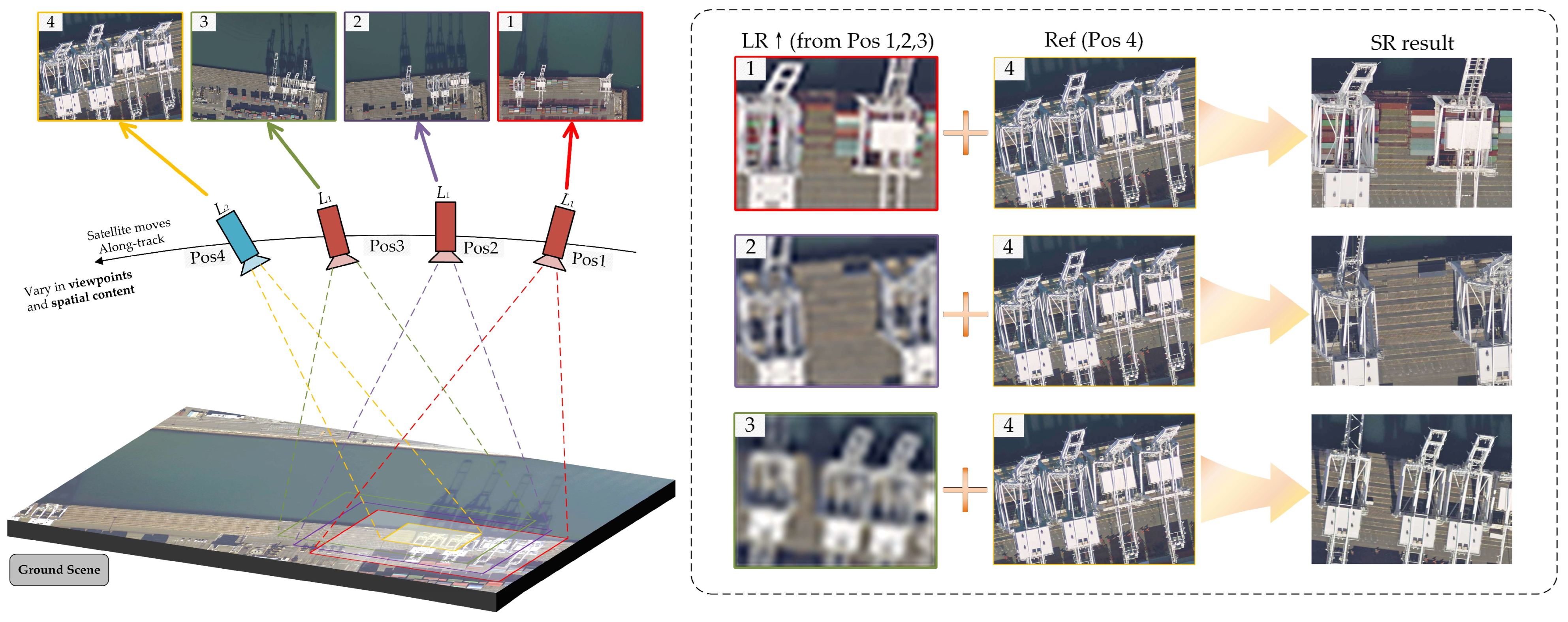
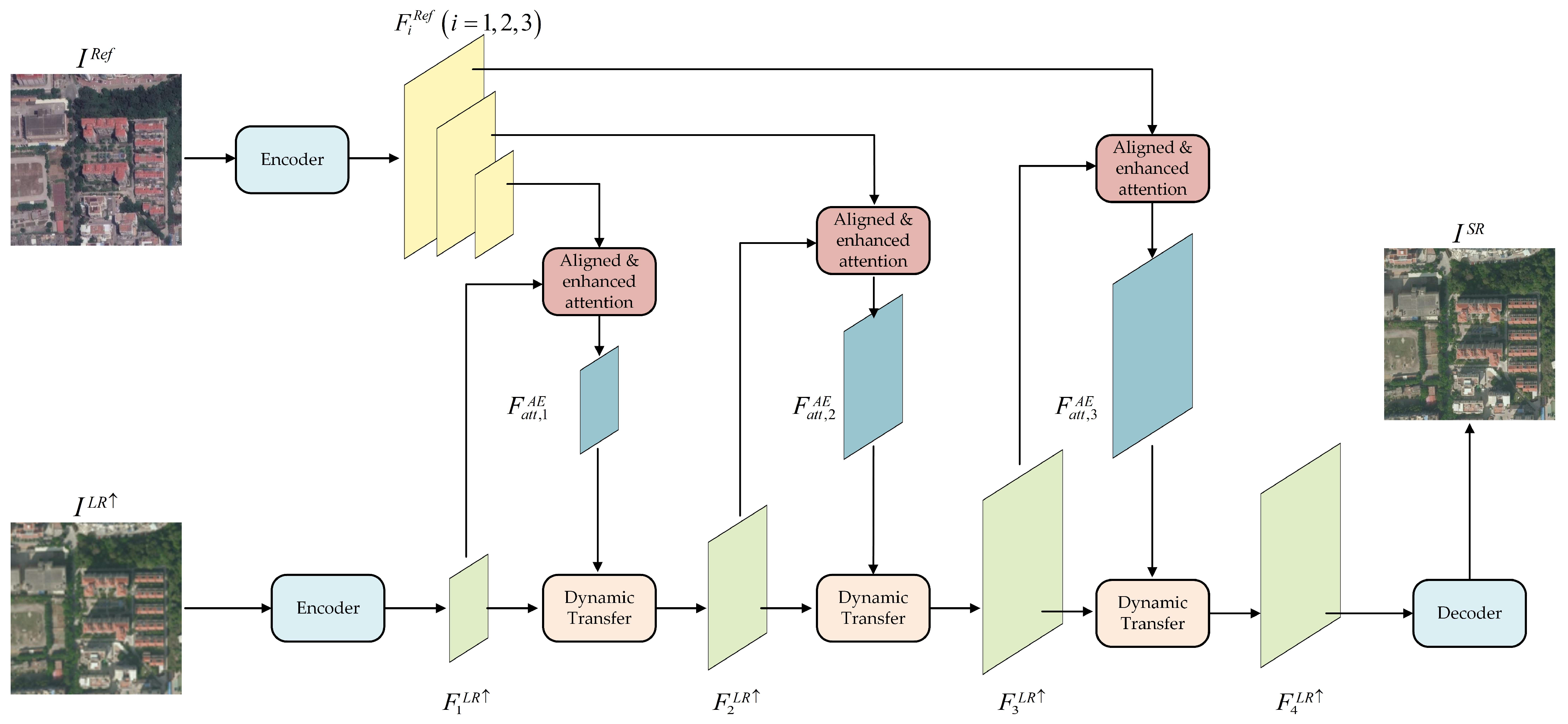
As shown in Figure 1, a zoom camera is installed and imaged towards a common region of interest (ROI). To fully estimate the effect of super resolution, the LR and Ref image are cropped from either camera imaging as shown in Figure 2, aligned with each other, and then super-resolved according to the proposed network AEFormer as shown in Figure 3. Given cameras with different focal lengths, L1 and L2, where L1 is equipped with the focal length of f while L2 is equipped with 4f, L1 and L2 are imaged towards the same target. LR is cropped from imagery by L1, with a size of n × n, while Ref is cropped from imagery by L2, with a size of 4n × 4n.
ZCS works following illustration in Figure 2. Constrained by the contradiction between the camera’s field of view (FOV) and imaging spatial resolution, for most cases, the zoom camera works as short-focus camera L1 to expand the effective imaging field, as shown in position 1,2,3. When encountering ROI, zoom camera changes focal length and works as long-focus camera L2 to obtain optical magnified image (Ref), as shown in position 4. With LR from Pos 1,2,3 and Ref from Pos 4 as inputs, corresponding SR im-ages can be obtained through the proposed AEFormer, as shown in right side of Figure 2.
Section 3 is arranged as follows. Section 3.1 introduces aligned and enhanced attention mechanism for feature alignment process. Section 3.2 presents feature transfer based on dynamic transfer module. Section 3.3 illustrates the loss function of the proposed AEFormer.

3.1. Feature Alignment Based on Aligned and Enhanced Attention

Considering the time intervals for changing the focal length of a zoom camera, there are subtle differences in the spatial content and viewpoint of images acquired by L1 and L2 which results in the misalignment problem between LR↑ and Ref. Addressing the misalignment is crucial for achieving a high-quality RefSR [11]. Since there is a certain similarity between patches across correlated images, the alignment strategy in the proposed network is based on the patch match [34].
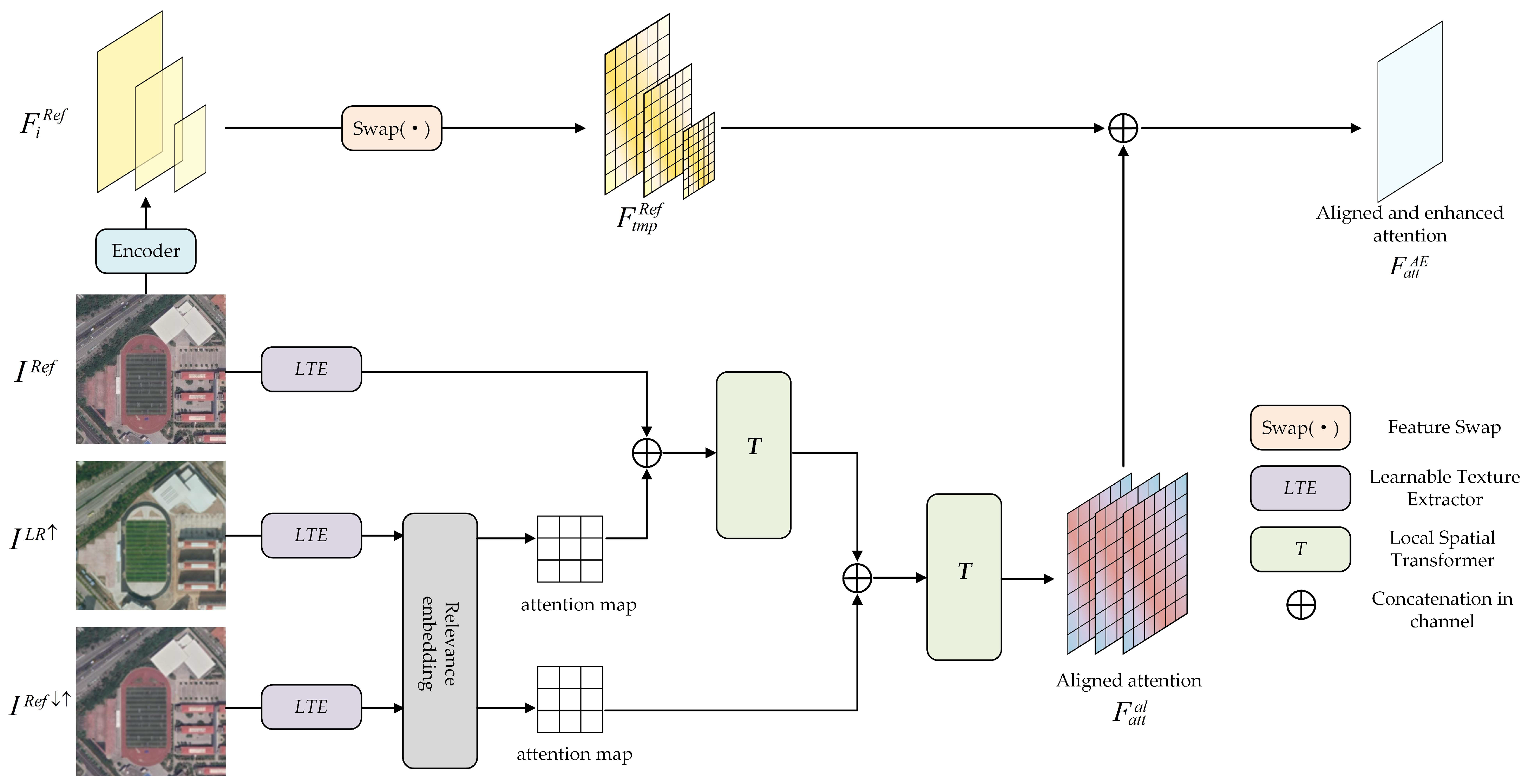
Different from previous patch-match-based methods where patches are swapped from non-learning process [13], the alignment strategy proposed in this study is an end-to-end ViT-based learnable process, namely of aligned and enhanced attention, as shown in Figure 4. For improved model generalization, Ref and LR, in this section, are selected from the external dataset which differ in spectral characteristics and spatial content despite being aimed for the same ROI. It corresponds to a normal RefSR verification process.
To bridge the gap between Ref and LR image, and obtain valid and effective aligned Ref features to be involved in SR reconstruction, it occurred to us that attention mechanism may be an alternative for deformable convolution [18] which is widely used in previous RefSR alignment practice [11], and the combination of feature swapping [13] and attention mechanism may lead to a reinforced aligned features acquisition. To obtain the mentioned aligned features, it takes several steps as follows.
First, considering there is a difference in content and viewpoint between LR↑ and Ref, Ref feature map FRef is swapped according to feature swapping [13], denoted as Swap(·), for a rough processing. The swapped Ref feature map F t m p R e f is only temporary because it does not involve a learning process.
F t m p R e f =   Swap F R e f
where the role of feature swap aims at swapping features which searches over the entire IRef for locally similar textures of ILR for enhanced SR reconstruction. The swapped LR and Ref patches, which may differ in color and illumination, are matched in neural feature space ϕ · [13] to emphasize the structural and textural information. The similarity between both can be calculated as:
s i , j = P i ϕ I L R , P j ϕ I R e f P j ϕ I R e f
where Pi denotes sampling i-th patch from corresponding feature map. si,j denotes the similarity between the i-th LR patch and the j-th Ref patch. The similarity computation Sj can be efficiently implemented as a set of convolution operations over all LR patches with each kernel corresponding to a Ref patch:
S j = ϕ I L R P j ϕ I R e f P j ϕ I R e f
where Sj denotes the similarity map for the j-th Ref patch, and * denotes the correlation operation. Use Sj (x, y) to denote the similarity between the LR patch centered at location (x, y) and the j-th Ref patch. Based on the similarity score, a swapped feature map M can be constructed to represent texture-enhanced LR image. Each patch in M centered at (x, y) is defined as
P ω ( x , y ) ( M ) = P j * ϕ I R e f , j * = arg max j S j ( x , y )
where ω x , y maps patch center to patch index. As a result, swapped feature map M can be obtained from feature swap, as the basis for subsequent operations.
Second, for all the image branches, including Ref image IRef, LR bicubic image ILR, and Ref down sampled then up sampled image IRef↓↑, the learnable texture extractor (LTE) [14] is adopted as the deep feature extractor of each branch. Once feature maps of three branches are obtained from LTE, they need to be aligned. For an improved alignment effect, Ref↓↑ and LR↑, which share the same image sampling frequency, need to be aligned first, which is different from previous alignment process [52]. Specifically, the relevance between Ref↓↑ and LR↑ images are calculated by relevance embedding [14,19,32]. Then, the embedded images I t m p R e f and I t m p L R are divided into patches pi and qi, in which p i   ( i [ 1 , H R e f × W R e f ] ) are from Ref↓↑ and q i   ( i [ 1 , H L R × W L R ] ) are from LR↑, respectively.
For each patch in I t m p R e f and I t m p L R , the relevance ri,j between two patches calculated by
r i , j = p i p i , q j q j R = r i , j 2
Third, through relevance map R obtained from Equation (5), the attention map can be achieved by incorporating the relevance map and feature map. Specifically, for Ref attention map, F t m p R e f and R R e f are integrated to obtain Ref attention map F a t t R e f :
F a t t R e f = T F t m p R e f   R R e f
where T denotes the local transformer network [53] which aims at estimating patch-wise alignment parameters for all patches. ⨁ denotes concatenation in channel. Similarly, for the LR↑ branch, F a t t R e f and R L R are incorporated to obtain the aligned attention F a t t a l :
F a t t a l = T F a t t R e f   R L R
Such aligned attention F a t t a l can compensate for the weakness of a swapped patch match feature map F t m p R e f where nonlinear misalignment is usually hard to cope with. However, non-learning feature map F t m p R e f contains a basic high-similarity patch match which means combining the strength of F t m p R e f and F a t t a l can hopefully enhance the aligned attention map F a t t a l . In this way, to further enhance F a t t a l , concatenate F t m p R e f and F a t t a l to obtain the final aligned and enhanced attention F a t t A E .
F a t t A E = F t m p R e f   F a t t a l
Compared with DATSR [35] where feature maps are obtained through convolution and aligned attention mechanism, this study enhanced the aligned attention on the basis on swapped features.
Based on the above process, F a t t A E can be transferred to the LR feature space to obtain the SR result through the proposed dynamic transfer module (DTM) in Section 3.2.

3.2. Feature Transfer Based on the Dynamic Transfer Module

Transferring an aligned feature to the LR feature space has been a long challenging task [11,54]. Direct transfer, such as summation or concatenation, would lead to information loss or misalignment.
To address the challenging task of feature transfer, this study proposes a novel dynamic transfer module (DTM), shown as Figure 5. From what is presented in Figure 3, aligned and enhanced attention F a t t A E is transferred to the LR feature space in a multi-level way. Within each level, DTM adopts the LR feature map F l e v e l L R and corresponding F a t t , l e v e l A E as inputs and generates F l e v e l + 1 L R as the output. The number of total levels corresponds to the number of feature encoding levels.
As shown in Figure 5, the transfer within each DTM can be divided into 3 stages. First, embed the concatenation between F a t t , l e v e l A E and F l e v e l L R with a learnable convolutional layer which is denoted as C1(·). The normalized attention map is then elementwise multiplied by the LR feature map. Second, obtain more information through another convolutional layer, which is denoted as C2, then elementwise add (denoted as +) that with the LR feature map. Finally, to obtain the output of DTM, the above attention map goes through residual blocks to prevent degradation resulting from multiple convolutions [20].
The above feature transfer process can be represented as
F l e v e l m u l =   Sig C 1 F l e v e l L R F a t t , l e v e l A E F l e v e l L R F l e v e l s u m =   C 2 F l e v e l m u l + F l e v e l L R F l e v e l + 1 L R =   Res F l e v e l s u m
where C1/2(·) denotes the learnable convolution layer with a kernel size of 3 × 3. Sig(·) denotes the sigmoid operation. Res(·) denotes residual blocks [20]. ⨁ denotes concatenation in the channel. ⨂ denotes elementwise multiplication. Level = 1, 2, and 3. Note that the output of DTM (level) equals the input of DTM (level + 1) which corresponds to Figure 3.
Furthermore, as can be seen from Figure 3 and Equation (9), F 4 L R can be obtained from the final level of feature transfer. With the decoder, the feature map F 4 L R can be transformed back to the image space, in other words, the SR result.

3.3. Loss Function

To achieve a better SR effect, the loss function in this study consists of four components which are reconstruction loss L r e c   , adversarial loss L a d v , perceptual loss L p e r   , and texture loss L t x t   . For improved clarity, the component and configuration of the loss function are different from previous studies [12,13,14,31].
L t o t a l   = λ r e c   L r e c   + λ a d v L a d v + λ p e r   L p e r   + λ t x t L t x t  
Reconstruction loss. To preserve the basic structure of LR-SR mapping, reconstruction loss aims at making SR infinitely approach HR (GT) during training. In this study, l1 norm is adopted within L r e c   . Notably, L r e c   is the most basic component of the SR training process.
L r e c   = I H R I S R l
Adversarial loss. Since GAN [24] is capable of reconstructing a visually satisfactory image, adversarial loss is common yet effective in recent SR tasks [11,31]. Herein, L a d v proposed in WGAN-GP [55] is adopted in our loss function.
L D = E x ˜ P g [ D ( x ˜ ) ] E x P r [ D ( x ) ] + λ E x ^ P x ^ x ^ D ( x ^ ) 2 1 2 L a d v = E x ˜ P g [ D ( x ˜ ) ]
where L D denotes loss of the discriminator. D(·) denotes 1-Lipschitz functions [56]. P r and P g denote the distribution of the proposed model and actual situation, respectively [14].
Perceptual loss. Inspired by [13,14,57,58], perceptual loss aiming for better visual perception, in our study, is different from previous studies. Specifically, L p e r   consists of two parts in this study. The first part is consistent with traditional studies while the second part combines the perceptual effect of an aligned and enhanced attention map because it records certain information of certain stages during training.
L p e r   = 1 C i H i W i ϕ i v g g I S R ϕ i v g g I H R 2 2 + 1 C j H j W j ϕ j E I S R F a t t A E 2 2
where ϕ i v g g represents the feature map of VGG-19 of the i-th layer while (Ci, Hi, Wi) represents the shape of the feature map. ISR denotes the super-resolved (generated) image of the corresponding iteration. ϕ j E denotes the feature map warped from the j-th layer of the rough alignment E(·) while F a t t A E denotes the aligned and enhanced attention of the corresponding iteration.
Texture loss. Following [13], texture loss, aimed at alleviating texture differences between ISR and IRef, is also involved in our loss function.
L t x t   = l λ l G r ϕ l I S R · S l * G r M l · S l * F
where Gr(·) computes the Gram matrix and λl is a normalization factor corresponding to the feature size of layer l. S l * denotes a weighting map for all LR patches.

4. Experiment

This section presents three aspects of our experiment. First, dataset and implementation details are presented as the basis of the experiment. Second, comparisons between state-of-the-art methods and ours are carried out for validating the effect of super-resolving. Finally, AEFormer’s capability of super-resolving real-world imagery is verified based on the proposed ZCS.

4.1. Dataset and Implementation Details

Dataset. To verify the effectiveness of the proposed method and train the proposed AEFormer, benchmark dataset RRSSRD [11] is adopted in our experiment. Specifically, 4047 pairs of HR-Ref remote sensing images are used for training while four groups of images are used for testing. RRSSRD is constructed based on GF-X satellite open source, Google Earth Engine, and Microsoft Virtual Earth, which contains various remote sensing scenes, such as urban architecture, an airport, farmland, a parking lot, and more. The spatial resolution of images from RRSSRD is approximately 0.5 m.
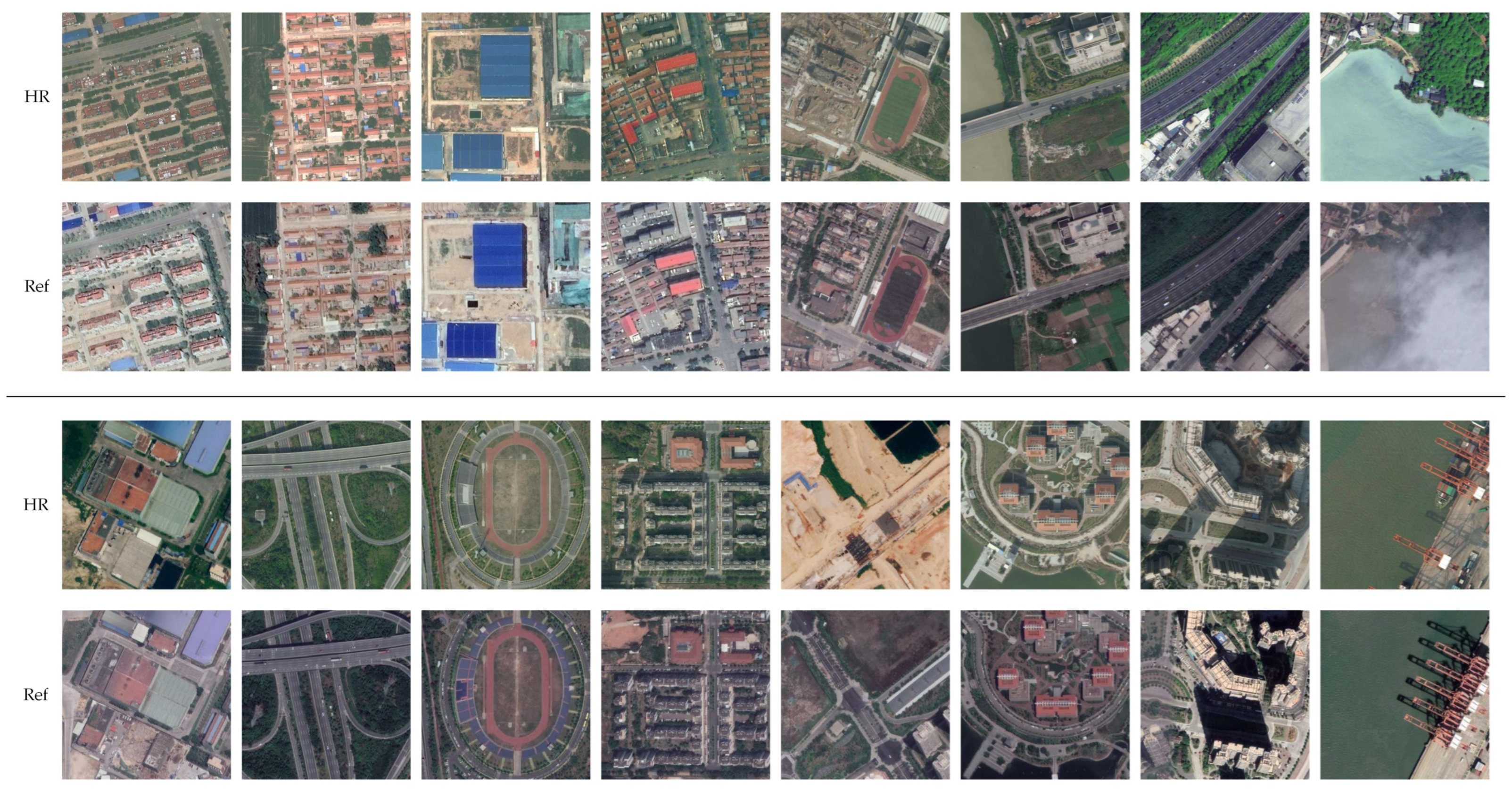
HR and Ref within RRSSRD have the same image resolution of 480 × 480 pixels, while LR is downsampled from HR with resolution of 120 × 120 (unit in pixel). Figure 6 displays some examples of HR-Ref pairs within RRSSRD. Following standard protocol in SR tasks [4,11,21], all LR images are obtained by bicubic downsampling corresponding HR images to a ¼ size. LR↑ denotes LR upsampling four times. Ref↓↑ denotes Ref downsampling then upsampling to the original size, which aims at seeking better matching band frequency between images [11,14], as shown in Figure 4.
In Section 4.2, LR (down sampled from HR) and Ref from RRSSRD test sets are used for a classical SR verification. In Section 4.3, LR and Ref are obtained from camera L1 and L2 (within ZCS) for real-world SR verification.
Implementation details. For a valid verification, following some previous known works [8,11,14,29], scale factor is set to be large as 4 in this study. For improved clarity, state-of-the-art methods are compared with the proposed AE-Former, including CNN-based SISR method EDSR [22], GAN-based SISR method SPSR [25], CNN-based RefSR method CrossNet [12], GAN-based RefSR method SRNTT [13], ViT-based SISR method SwinIR [41], ViT-based RefSR method TTSR [14]. For fair comparison, all methods are configured via the default provided by their authors to achieve their best performance and trained for a consistent or close iteration. AEFormer is trained for 200,000 iterations to achieve convergence, which took about 53 h on 2 × Nvidia RTX 4090. SRNTT was implemented on TensorFlow while others were implemented on PyTorch. Inspired by some previous known works [11,15,25,41,52,59,60], hyperparameter configuration in our study, which are ( L r e c   , L p e r   , L a d v , L t x t   ) in Equation (10), are set as 1, 1 × 10⁻³, 1.5 × 10⁻⁷, and 1 × 10⁻⁷, respectively. Quantitative comparison between state-of-the-art methods and AEFormer in Section 4.2 are evaluated in terms of LPIPS [61], PSNR, SSIM, and FID [62,63,64], all of which compare SR with HR (GT) to calculate the corresponding evaluation metrics. For real-world experimentation in Section 4.3, SR quality is evaluated by NIQE [65] and PI [23], both of which are non-reference image quality evaluation metrics [66]. Besides, the metrics for evaluating the diversity of GAN capability, IS, is also adopted in the comparison study [64].
LPIPS I S R , I 0 = l 1 H l W l h , w w l y ^ h w l y ^ 0 h w l 2 2 PI   = 1 2 10 Ma + NIQE FID P r , P g = μ r μ g + Tr C r + C g 2 C r C g 1 / 2 IS P g = e E x P g K L p M ( y x ) p M ( y )
where Hl and Wl represent the height and width of l-th layer. y ^ h w l and y ^ 0 h w l indicate the features at the specific location (h, w) of l-th layer from the generated image and the ground truth image. wl is a supervised weight vector. ⊙ denotes elementwise multiply. Tr(∙) represents the sum of elements on the diagonal of a matrix. PI, as the non-reference metrics, can be calculated by incorporating the criteria of Ma [67] and NIQE [65]. It indicates the perception quality of the generated image. More details in the generated image can lead to a better PI result, which is lower in score. In FID equation, the distance between these two univariate Gaussian distributions is calculated using mean and variance, in which r denotes the ground-truth image, while g denotes the generated image. A lower FID means that the two distributions are closer, which means that the quality and diversity of the generated images are higher. Lastly, in IS equation, the conditional probability P(y|x) is expected to be highly predictable (low entropy) for GAN. For example, given an image, the object type should be known easily. In turn, an Inception network is used to classify the generated images and predict P(y|x), where y is the label and x is the generated data. This reflects the quality of the images. Besides, if the generated images are diverse, the data distribution for y should be uniform (high entropy) [64]. Finally, to combine these two criteria (quality and diversity), their KL-divergence can be computed and the equation can be used to obtain IS score. Based on previous knowledge [63] and experimental results below, the biggest difference between FID and IS is that FID focuses more on image similarity, while IS focuses more on data diversity especially for GAN methods.

4.2. Comparison with State-of-the-Art Methods

In this section, both qualitative and quantitative comparisons are carried out to fully estimate the performance of the proposed AEFormer.
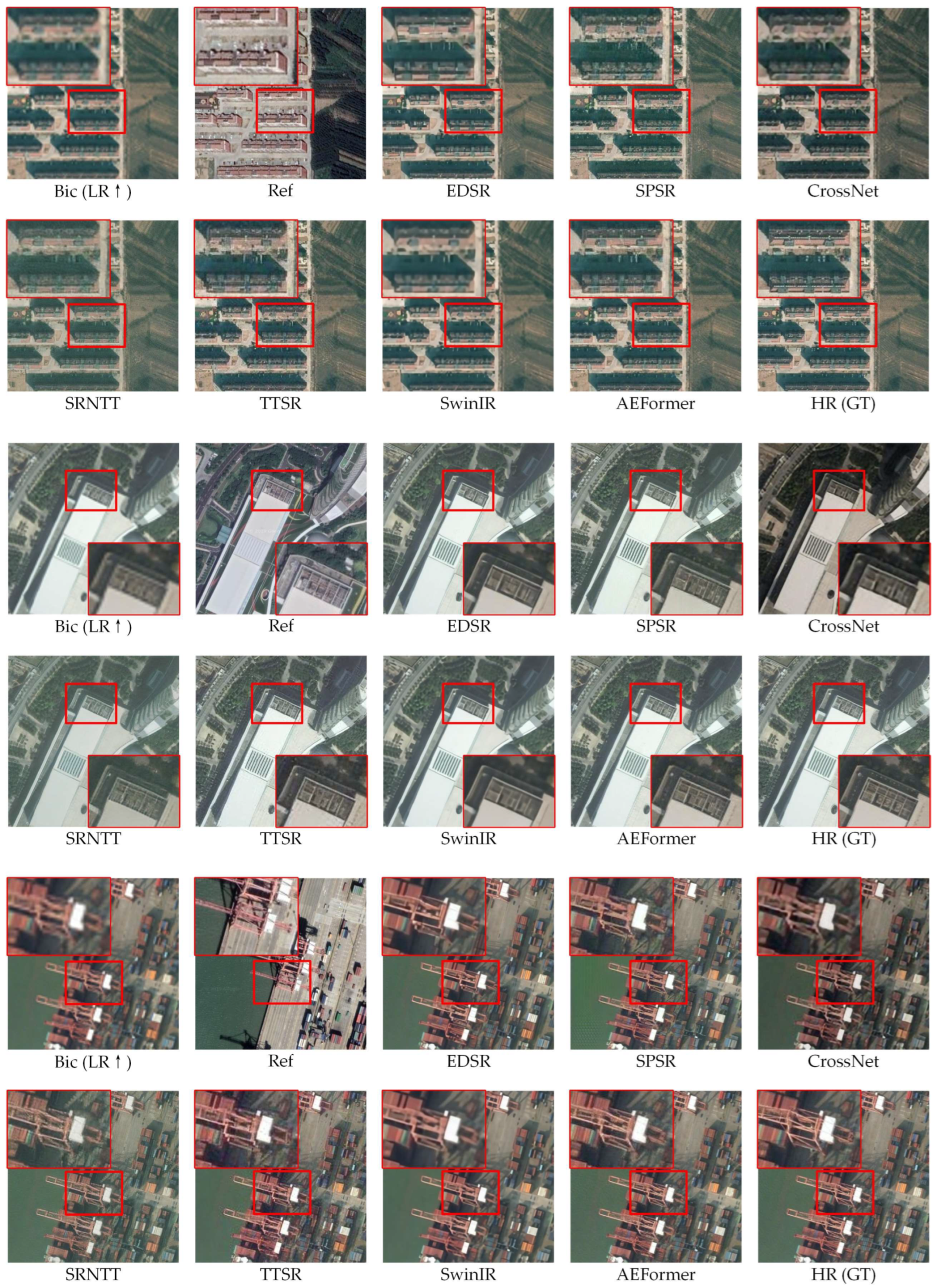
Qualitative comparison. To verify the visual quality of SR results, AEFormer is compared to state-of-the-art methods. As shown in Figure 7, AEFormer elicits the best visual quality on the dis-played test sets. It’s also observable that, by enriching details from Ref, RefSR methods are more visually satisfactory than SISR methods. Although Ref and HR differ in viewpoints, spectral characteristics, and spatial content within RRSSRD, AEFormer successfully utilizes Ref and LR to reconstruct the best SR effect among selected methods. Specifically, in the first set in Figure 7, AEFormer retains the best roof details while suppressing noise across whole image (compared to TTSR). In the second set, only AEFormer recovers the horizontal structures. In the third set, SPSR and TTSR generate massive artifacts and blurriness on the scaffolding, while other methods even fail to distinguish between multiple scaffolding elements. Only AEFormer succeeds in distinguishing them.
It’s observable that SwinIR, which is trained with reconstruction only, achieves the second best PSNR and SSIM scores, only second to AEFormer_rec (AEFormer trained from scratch with reconstruction loss only). Based on previous known studies [11,13,14], it’s commonly known that SR network trained with reconstruction loss (e.g. l1 loss) can lead to better PSNR and SSIM scores, because they’re usually oriented towards MAE or MSE. However, higher PSNR and SSIM don’t guarantee a better visual result because over-smooth texture can lead to higher PSNR, this is why we need different loss functions and additional metrics to evaluate its effectiveness.
Quantitative comparison. Table 1 shows the quantitative comparison on RRSSRD in terms of LPIPS, PI, NIQE, FID, IS, PSNR, and SSIM. Red bold score denotes the 1st best result, while blue bold score denotes the second best result. Considering the combination of different loss functions con-tribute to a more photo-realistic details with slightly worse PSNR and SSIM score [11,21], AEFormer is trained from scratch with all losses, denoted as AEFormer. For fair comparison, AEFormer is additionally trained with reconstruction loss only to achieve higher PSNR and SSIM score, with adversarial loss, perceptual loss and texture loss removed, which is denoted as AEFormer_rec.
It’s observable that AEFormer outperforms the second best method, SwinIR [41], 53.28%, 1.98%, 2.14% in terms of average LPIPS, PNSR, and SSIM. It further reiterates the superiority of AEFormer. Considering there are many indicators in this section, some of which are lower, the better, whereas for others is the opposite.
For more intuitive com-parison, improvement percentage in this study is defined as
Improvement   Percentage = I n d i c a t o r ( M e t h o d ) I n d i c a t o r ( B i c ) I n d i c a t o r ( B i c ) × 100 %
For each indicator in Table 1, denote the improvement of each average indicator of the compared methods by calculating corresponding improvement percentage. The higher the percentage is, the more effective corresponding method is. The graphical result of improvement percentage is shown in Figure 8. It’s observable that the pro-posed AEFormer (and AEFormer_rec) can elicit the best improvement percentage in most circumstances.

4.3. ZCS for Real-World Super Resolution

The above experiment adopts degraded images (LR down sampled from HR) as LR to verify the effectiveness of AEFormer. This typical super-resolution verification differs from super-resolving real-world data because real-world LR data are not obtained through down sampling. Since there is no equivalent corresponding HR (GT) of real-world LR data, the quality of SR results cannot be evaluated by previous metrics which are LPIPS, PSNR, and SSIM. Instead, they should be evaluated by PI [23] and NIQE [65], both of which are non-reference image quality evaluation metrics [66]. In this section, SR results of real-world Orbita satellite data [68] are verified.
The experimental process of super-resolving real-world data based on ZCS also follows the flowchart outlined in Figure 1. Evidently, as shown in Figure 9, short-focus camera L1 is aimed for capturing the wide FOV image where LR images are cropped from. Long-focus camera L2, with limited and narrow FOV, is aimed for obtaining Ref images, which share the same image resolution as LR↑. In this section, both LR↑ and Ref have the same image resolution as 600 × 600 (unit in pixel).
Although Orbita satellite data are not involved in our training, the SR result of AEFormer still elicits the best performance both qualitatively and quantitatively when compared with the selected state-of-the-art methods.
As shown in Figure 9, the SR image of SPSR is full of noise and artifacts. On one hand, the SR image of SRNTT lacks real image intensity despite achieving the second best scores. On the other hand, SwinIR, trained only on reconstruction loss, achieves low scores when facing real-world imagery super resolution, which is different from the previous section. It proves the necessity of a combination of different loss functions, especially perceptual loss and adversarial loss. Most importantly, the SR image of AEFormer shows the most detailed contents and achieves the best scores in terms of PI and NIQE (Table 2). It demonstrates the robustness and effectiveness of the proposed method.

5. Discussion

In this section, three key points of the proposed method, which are ZCS, aligned and enhanced attention, and dynamic transfer module, are discussed. Specifically, the implementation process of ZCS is discussed. Its current effectiveness and future development are detailed. Additionally, ablation studies are carried out on the aligned and enhanced attention and dynamic transfer module to demonstrate their effectiveness.

5.1. Effectiveness and Limitation of ZCS

As introduced in Section 2.2, the performance of RefSR greatly depends on the alignment between the LR and Ref image. In other words, it also indicates that the quality of the Ref image could possibly affect the performance of RefSR. In the proposed ZCS, zoom camera L2 is equipped with four times the focal length of L1 to obtain the magnified yet same resolution Ref image as LR↑. What would happen when L2 is equipped with different focal lengths? Moreover, what would happen when an irrelevant image or external dataset is adopted as a Ref for the RefSR process?
To verify the necessity and effectiveness of ZCS, an ablation study is carried out on the quality of Ref which is photographed by zoom camera L2. Specifically, to address the above questions, two types of experiments are conducted. First, adopt a different focal length to obtain a different Ref image, which captures different regions from LR↑ or the previous Ref. Second, adopt an irrelevant image or external dataset as the Ref. By comparing corresponding SR results based on the above Ref both qualitatively and quantitatively, a comprehensive conclusion about the effectiveness of the proposed ZCS can be arrived at.
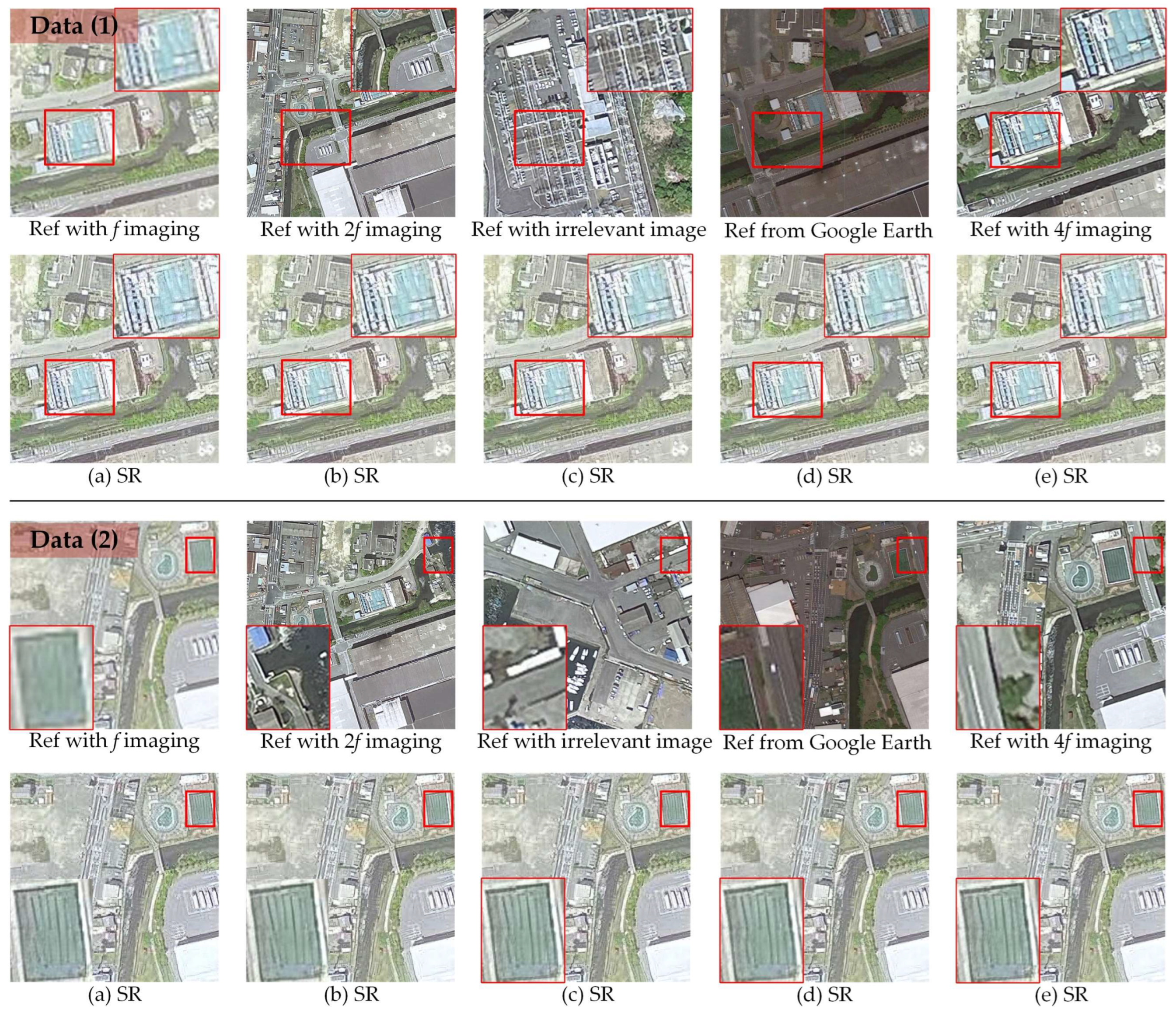
As shown in Figure 10 and Table 3, different ZCS configurations result in obtaining different Ref images, in turn leading to different SR results. By evaluating corresponding SR results, the effectiveness of ZCS can be estimated. Specifically, given a fixed L1 configuration (f), different ZCS configurations include L2 imaging with focal lengths of f, 2f, and 4f. Moreover, irrelevant imagery and external datasets (from Google Earth Engine 2023) are also involved in ZCS configurations.
It can be concluded from Figure 10 and Table 3 that adopting Google Earth data and L2 4f imaging as Ref can possibly lead to the best SR result while adopting L2 f imaging or irrelevant imagery as the Ref leads to a poor SR result. This is possibly due to the high-frequency details in Ref because there are many high-frequency details in Ref from L2 4f imaging whereas there are few in Ref from L2 f imaging. Since the external dataset may vary significantly from LR in spatial content or other issues, ZCS for capturing ahigh-quality Ref proves feasibly accessible and practically effective for contributing to a better RefSR performance. In remote sensing practice, determining which Ref, from 4f ZCS or Google Earth, to use depends on data accessibility.
In future remote sensing practice, common path system [69,70] can be introduced into satellite camera design for shortening the interval time of the changing focal length.

5.2. Effectiveness of Aligned and Enhanced Attention

In this study, the remarkable performance of the proposed AEFormer is attributed to the configuration of Ref↓↑ branch, aligned attention, and aligned and enhanced attention, all of which are regarded as improvements from previous studies [14,25,31,41,71]. To verify the necessity and importance of these modules, ablation study is carried out on each mod-ule, as shown in Table 4.
Notably, ‘Ref↓↑ branch’, ‘Aligned attention’, and ‘Enhanced attention’ in Table 4 are not complementary. For ‘Ref↓↑ branch’, × denotes removing the Ref↓↑ branch in Figure 4 while √ denotes reserving this branch. ‘Aligned attention’ is the basis of ‘Enhanced attention’, which means the existence of enhanced attention depends on the existence of aligned attention in Figure 4.
It can be seen from the first row and second row within Table 4 that the existence of aligned attention contributes to an improvement among all scores significantly where LPIPS, PSNR, and SSIM are improved by 13.8%, 3.27%, and 2.70%, respectively. Moreover, given a considerable improvement among all metrics from the second and third row, it verifies the necessity of the Ref↓↑ branch. Furthermore, based on the third row and last row, the existence of aligned and enhanced attention leads to further improvements in LPIPS and SSIM despite a slight and acceptable decrease in PSNR. It indicates that the proposed aligned and enhanced attention fully exploit and utilize the feature space to release the potential for a more effective alignment process.

5.3. Effectiveness of Dynamic Transfer Module

To further verify the effectiveness of transfer process (in this study in DTM), ablation study is carried out on transfer module. There’re many fusion-based and transfer-based methods currently [36,37,38]. Different from these studies, the proposed DTM consists of sigmoid module and convolution module, while DTM is used in each level of aligned Ref features transferring. In this way, ablation study is carried out on sigmoid part (for generating a learning mask) and convolution part (for extracting and rein-forcing features). It’s observable from Table 5 that removing sigmoid part leads to approximately 13.5% decrease in terms of LPIPS, 4.4% decrease in PSNR, and 5.5% decrease in SSIM. It’s also observable that removing convolution part leads to a slightly mild decrease. It verifies the necessity and effectiveness of the components within DTM.

6. Conclusions

This study presents a novel method for achieving better RefSR performance in the field of remote sensing by exploring a novel imaging mode, namely ZCS, and a novel algorithm, namely AEFormer, in which ZCS serves as the structural basis for implementing AEFormer. On one hand, ZCS utilizes the magnification performance of the zoom camera to obtain a high-quality Ref image with the least temporal and spatial redundancy. On the other hand, AEFormer, with highlights in aligned and enhanced attention and dynamic transfer, achieves state-of-the-art performance among the selected SISR and RefSR methods. Aligned and enhanced attention prove superior to previous alignment modules which should be an enlightenment for future alignment module design. This study, with its blend of theoretical innovation and engineering applicability, proves potentially impactful for future remote sensing imaging.
In the future, efforts will be made towards optimizing the model, for example, introducing a semi-supervised mechanism into the loss function for improved learning effectiveness.

Author Contributions

Conceptualization, Z.T. and X.Y.; methodology, Z.T. and Z.F.; software, Z.T.; validation, Z.T., X.T., X.H. and T.X.; formal analysis, Z.T., Z.F. and X.T.; investigation, Z.T. and X.T.; resources, Z.T., P.L. and L.J.; data curation, Z.T. and Z.F.; writing—original draft preparation, Z.T.; writing—review and editing, Z.T., Z.F., T.X., X.H. and X.T.; visualization, Z.T.; supervision, Z.T. and X.Y.; project administration, Z.T.; funding acquisition, X.Y. All authors have read and agreed to the published version of the manuscript.

Funding

This work was supported in part by Key Research and Development Program of Jilin Province under Grant 20230201061GX, in part by Natural Science Foundation of Jilin Province under Grant 20210101099JC, in part by National Natural Science Foundation of China under Grant 62171430, in part by National Natural Science Foundation of China under Grant 62101071, in part by Entrepreneurship Team Project of Zhuhai City under Grant ZH0405190001PWC.

Data Availability Statement

The data of experimental images used to support the findings of this research are available from the corresponding author upon reasonable request.

Acknowledgments

The authors are sincerely grateful for the constructive comments and suggestions of the manuscript reviewers.

Conflicts of Interest

The authors declare no conflict of interest.

Abbreviations

The following abbreviations are used in this paper:
AbbreviationFull Name
SRSuper resolution
LRLow resolution
RefReference (image)
HRHigh resolution
GTGround truth
ViTVision transformer
LTELearnable texture extractor
ZCSZoom camera structure
FOVField of view
SISRSingle-image super resolution
Ref-SRReference-based super resolution
CNNConvolutional neural network
GANGenerative adversarial network
AEFormerReference-based super-resolution network via aligned and enhanced attention

References

  1. Tsai, R.Y.; Huang, T.S. Multiframe image restoration and registration. Multiframe Image Restor. Regist. 1984, 1, 317–339. [Google Scholar]
  2. Zhang, H.; Yang, Z.; Zhang, L.; Shen, H. Super-Resolution Reconstruction for Multi-Angle Remote Sensing Images Considering Resolution Differences. Remote Sens. 2014, 6, 637–657. [Google Scholar] [CrossRef]
  3. Dong, C.; Loy, C.C.G.; He, K.M.; Tang, X.O. Learning a Deep Convolutional Network for Image Super-Resolution. In Proceedings of the 13th European Conference on Computer Vision (ECCV), Zurich, Switzerland, 6–12 September 2014; pp. 184–199. [Google Scholar]
  4. Dong, C.; Loy, C.C.; He, K.M.; Tang, X.O. Image Super-Resolution Using Deep Convolutional Networks. IEEE Trans. Pattern Anal. Mach. Intell. 2016, 38, 295–307. [Google Scholar] [CrossRef] [PubMed]
  5. Zhao, M.H.; Ning, J.W.; Hu, J.; Li, T.T. Hyperspectral Image Super-Resolution under the Guidance of Deep Gradient Information. Remote Sens. 2021, 13, 2382. [Google Scholar] [CrossRef]
  6. Xu, Y.Y.; Luo, W.; Hu, A.N.; Xie, Z.; Xie, X.J.; Tao, L.F. TE-SAGAN: An Improved Generative Adversarial Network for Remote Sensing Super-Resolution Images. Remote Sens. 2022, 14, 2425. [Google Scholar] [CrossRef]
  7. Guo, M.Q.; Zhang, Z.Y.; Liu, H.; Huang, Y. NDSRGAN: A Novel Dense Generative Adversarial Network for Real Aerial Imagery Super-Resolution Reconstruction. Remote Sens. 2022, 14, 1574. [Google Scholar] [CrossRef]
  8. Wang, P.J.; Bayram, B.; Sertel, E. A comprehensive review on deep learning based remote sensing image super-resolution methods. Earth-Sci. Rev. 2022, 232, 25. [Google Scholar] [CrossRef]
  9. Singla, K.; Pandey, R.; Ghanekar, U. A review on Single Image Super Resolution techniques using generative adversarial network. Optik 2022, 266, 31. [Google Scholar] [CrossRef]
  10. Qiao, C.; Li, D.; Guo, Y.T.; Liu, C.; Jiang, T.; Dai, Q.H.; Li, D. Evaluation and development of deep neural networks for image super-resolution in optical microscopy. Nat. Methods 2021, 18, 194–202. [Google Scholar] [CrossRef]
  11. Dong, R.; Zhang, L.; Fu, H. RRSGAN: Reference-Based Super-Resolution for Remote Sensing Image. IEEE Trans. Geosci. Remote Sens. 2022, 60, 5601117. [Google Scholar] [CrossRef]
  12. Zheng, H.T.; Ji, M.Q.; Wang, H.Q.; Liu, Y.B.; Fang, L. CrossNet: An End-to-End Reference-Based Super Resolution Network Using Cross-Scale Warping. In Proceedings of the 15th European Conference on Computer Vision (ECCV), Munich, Germany, 8–14 September 2018; pp. 87–104. [Google Scholar]
  13. Zhang, Z.F.; Wang, Z.W.; Lin, Z.; Qi, H.R. Image Super-Resolution by Neural Texture Transfer. In Proceedings of the 32nd IEEE/CVF Conference on Computer Vision and Pattern Recognition (CVPR), Long Beach, CA, USA, 16–20 June 2019; pp. 7974–7983. [Google Scholar]
  14. Yang, F.Z.; Yang, H.; Fu, J.L.; Lu, H.T.; Guo, B.N. Learning Texture Transformer Network for Image Super-Resolution. In Proceedings of the IEEE/CVF Conference on Computer Vision and Pattern Recognition (CVPR), Electr Network, Seattle, WA, USA, 14–19 June 2020; pp. 5790–5799. [Google Scholar]
  15. Wang, T.; Xie, J.; Sun, W.; Yan, Q.; Chen, Q. Dual-camera super-resolution with aligned attention modules. In Proceedings of the IEEE/CVF International Conference on Computer Vision, Montreal, BC, Canada, 11–17 October 2021; pp. 2001–2010. [Google Scholar]
  16. Zhang, Y.F.; Li, T.R.; Zhang, Y.; Chen, P.R.; Qu, Y.F.; Wei, Z.Z. Computational Super-Resolution Imaging with a Sparse Rotational Camera Array. IEEE Trans. Comput. Imaging 2023, 9, 425–434. [Google Scholar] [CrossRef]
  17. Liu, S.-B.; Xie, B.-K.; Yuan, R.-Y.; Zhang, M.-X.; Xu, J.-C.; Li, L.; Wang, Q.-H. Deep learning enables parallel camera with enhanced- resolution and computational zoom imaging. PhotoniX 2023, 4, 17. [Google Scholar] [CrossRef]
  18. Zhu, X.Z.; Hu, H.; Lin, S.; Dai, J.F. Deformable ConvNets v2: More Deformable, Better Results. In Proceedings of the IEEE/CVF Conference on Computer Vision and Pattern Recognition (CVPR), Long Beach, CA, USA, 16–20 June 2019; pp. 9300–9308. [Google Scholar]
  19. Vaswani, A.; Shazeer, N.; Parmar, N.; Uszkoreit, J.; Jones, L.; Gomez, A.N.; Kaiser, L.; Polosukhin, I. Attention Is All You Need. In Proceedings of the 31st Annual Conference on Neural Information Processing Systems (NIPS), Long Beach, CA, USA, 4–9 December 2017. [Google Scholar]
  20. He, K.M.; Zhang, X.Y.; Ren, S.Q.; Sun, J. Deep Residual Learning for Image Recognition. In Proceedings of the 2016 IEEE Conference on Computer Vision and Pattern Recognition (CVPR), Seattle, WA, USA, 27–30 June 2016; pp. 770–778. [Google Scholar]
  21. Ledig, C.; Theis, L.; Huszar, F.; Caballero, J.; Cunningham, A.; Acosta, A.; Aitken, A.; Tejani, A.; Totz, J.; Wang, Z.H.; et al. Photo-Realistic Single Image Super-Resolution Using a Generative Adversarial Network. In Proceedings of the 30th IEEE/CVF Conference on Computer Vision and Pattern Recognition (CVPR), Honolulu, HI, USA, 21–26 July 2017; pp. 105–114. [Google Scholar]
  22. Lim, B.; Son, S.; Kim, H.; Nah, S.; Lee, K.M. Enhanced Deep Residual Networks for Single Image Super-Resolution. In Proceedings of the 30th IEEE/CVF Conference on Computer Vision and Pattern Recognition Workshops (CVPRW), Honolulu, HI, USA, 21–26 July 2017; pp. 1132–1140. [Google Scholar]
  23. Blau, Y.; Mechrez, R.; Timofte, R.; Michaeli, T.; Zelnik-Manor, L. The 2018 PIRM Challenge on Perceptual Image Super-Resolution. In Proceedings of the 15th European Conference on Computer Vision (ECCV), Munich, Germany, 8–14 September 2018; pp. 334–355. [Google Scholar]
  24. Goodfellow, I.; Pouget-Abadie, J.; Mirza, M.; Xu, B.; Warde-Farley, D.; Ozair, S.; Courville, A.; Bengio, Y. Generative Adversarial Networks. Commun. ACM 2020, 63, 139–144. [Google Scholar] [CrossRef]
  25. Ma, C.; Rao, Y.M.; Lu, J.W.; Zhou, J. Structure-Preserving Image Super-Resolution. IEEE Trans. Pattern Anal. Mach. Intell. 2022, 44, 7898–7911. [Google Scholar] [CrossRef]
  26. Liu, J.; Yuan, Z.; Pan, Z.; Fu, Y.; Liu, L.; Lu, B. Diffusion Model with Detail Complement for Super-Resolution of Remote Sensing. Remote Sens. 2022, 14, 4834. [Google Scholar] [CrossRef]
  27. Han, L.; Zhao, Y.; Lv, H.; Zhang, Y.; Liu, H.; Bi, G.; Han, Q. Enhancing Remote Sensing Image Super-Resolution with Efficient Hybrid Conditional Diffusion Model. Remote Sens. 2023, 15, 3452. [Google Scholar] [CrossRef]
  28. Yuan, Z.; Hao, C.; Zhou, R.; Chen, J.; Yu, M.; Zhang, W.; Wang, H.; Sun, X. Efficient and Controllable Remote Sensing Fake Sample Generation Based on Diffusion Model. IEEE Trans. Geosci. Remote Sens. 2023, 61, 1–12. [Google Scholar] [CrossRef]
  29. Jiang, Y.M.; Chan, K.C.K.; Wang, X.T.; Loy, C.C.; Liu, Z.W. Robust Reference-based Super-Resolution via C-2-Matching. In Proceedings of the IEEE/CVF Conference on Computer Vision and Pattern Recognition (CVPR), Electr Network, Virtual, 19–25 June 2021; pp. 2103–2112. [Google Scholar]
  30. Shim, G.; Park, J.; Kweon, I.S. Robust reference-based super-resolution with similarity-aware deformable convolution. In Proceedings of the IEEE/CVF Conference on Computer Vision and Pattern Recognition, Seattle, WA, USA, 13–19 June 2020; pp. 8425–8434. [Google Scholar]
  31. Zhang, J.Y.; Zhang, W.X.; Jiang, B.; Tong, X.D.; Chai, K.Y.; Yin, Y.C.; Wang, L.; Jia, J.H.; Chen, X.X. Reference-Based Super-Resolution Method for Remote Sensing Images with Feature Compression Module. Remote Sens. 2023, 15, 1103. [Google Scholar] [CrossRef]
  32. Lu, L.Y.; Li, W.B.; Tao, X.; Lu, J.B.; Jia, J.Y. MASA-SR: Matching Acceleration and Spatial Adaptation for Reference-Based Image Super-Resolution. In Proceedings of the IEEE/CVF Conference on Computer Vision and Pattern Recognition (CVPR), Electr Network, Virtual, 19–25 June 2021; pp. 6364–6373. [Google Scholar]
  33. Chen, T.Q.; Schmidt, M. Fast patch-based style transfer of arbitrary style. arXiv 2016, arXiv:1612.04337. [Google Scholar]
  34. Barnes, C.; Shechtman, E.; Finkelstein, A.; Goldman, D.B. PatchMatch: A Randomized Correspondence Algorithm for Structural Image Editing. ACM Trans. Graph. 2009, 28, 11. [Google Scholar] [CrossRef]
  35. Cao, J.Z.; Liang, J.Y.; Zhang, K.; Li, Y.W.; Zhang, Y.L.; Wang, W.G.; Van Gool, L. Reference-Based Image Super-Resolution with Deformable Attention Transformer. In Proceedings of the 17th European Conference on Computer Vision (ECCV), Tel Aviv, Israel, 23–27 October 2022; pp. 325–342. [Google Scholar]
  36. Zhou, R.; Zhang, W.; Yuan, Z.; Rong, X.; Liu, W.; Fu, K.; Sun, X. Weakly Supervised Semantic Segmentation in Aerial Imagery via Explicit Pixel-Level Constraints. IEEE Trans. Geosci. Remote Sens. 2022, 60, 1–17. [Google Scholar] [CrossRef]
  37. Yuan, Z.; Zhang, W.; Tian, C.; Mao, Y.; Zhou, R.; Wang, H.; Fu, K.; Sun, X. MCRN: A Multi-source Cross-modal Retrieval Network for remote sensing. Int. J. Appl. Earth Obs. Geoinf. 2022, 115, 103071. [Google Scholar] [CrossRef]
  38. Yuan, Z.; Zhang, W.; Tian, C.; Rong, X.; Zhang, Z.; Wang, H.; Fu, K.; Sun, X. Remote Sensing Cross-Modal Text-Image Retrieval Based on Global and Local Information. IEEE Trans. Geosci. Remote Sens. 2022, 60, 1–16. [Google Scholar] [CrossRef]
  39. Dosovitskiy, A.; Fischer, P.; Ilg, E.; Hausser, P.; Hazirbas, C.; Golkov, V.; van der Smagt, P.; Cremers, D.; Brox, T. FlowNet: Learning Optical Flow with Convolutional Networks. In Proceedings of the IEEE International Conference on Computer Vision, Santiago, Chile, 11–18 December 2015; pp. 2758–2766. [Google Scholar]
  40. Simonyan, K.; Zisserman, A. Very Deep Convolutional Networks for Large-Scale Image Recognition. arXiv 2015, arXiv:1409.1556. [Google Scholar]
  41. Liang, J.Y.; Cao, J.Z.; Sun, G.L.; Zhang, K.; Van Gool, L.; Timofte, R. SwinIR: Image Restoration Using Swin Transformer. In Proceedings of the 18th IEEE/CVF International Conference on Computer Vision (ICCV), Electr Network, Montreal, BC, Canada, 11–17 October 2021; pp. 1833–1844. [Google Scholar]
  42. Lu, Z.S.; Li, J.C.; Liu, H.; Huang, C.Y.; Zhang, L.L.; Zeng, T.Y. Transformer for Single Image Super-Resolution. In Proceedings of the IEEE/CVF Conference on Computer Vision and Pattern Recognition (CVPR), New Orleans, LA, USA, 18–24 June 2022; pp. 456–465. [Google Scholar]
  43. Wu, H.P.; Xiao, B.; Codella, N.; Liu, M.C.; Dai, X.Y.; Yuan, L.; Zhang, L. CvT: Introducing Convolutions to Vision Transformers. In Proceedings of the 18th IEEE/CVF International Conference on Computer Vision (ICCV), Electr Network, Montreal, BC, Canada, 11–17 October 2021; pp. 22–31. [Google Scholar]
  44. Chen, X.; Wang, X.; Zhou, J.; Dong, C. Activating More Pixels in Image Super-Resolution Transformer. arXiv 2022, arXiv:2205.04437v3. [Google Scholar]
  45. Grosche, S.; Regensky, A.; Seiler, J.; Kaup, A. Image Super-Resolution Using T-Tetromino Pixels. arXiv 2023, arXiv:2111.09013. [Google Scholar]
  46. Ma, J.Y.; Tang, L.F.; Fan, F.; Huang, J.; Mei, X.G.; Ma, Y. SwinFusion: Cross-domain Long-range Learning for General Image Fusion via Swin Transformer. IEEE-CAA J. Autom. Sin. 2022, 9, 1200–1217. [Google Scholar] [CrossRef]
  47. Wilburn, B.; Joshi, N.; Vaish, V.; Talvala, E.V.; Antunez, E.; Barth, A.; Adams, A.; Horowitz, M.; Levoy, M. High performance imaging using large camera arrays. ACM Trans. Graph. 2005, 24, 765–776. [Google Scholar] [CrossRef]
  48. Yu, S.; Moon, B.; Kim, D.; Kim, S.; Choe, W.; Lee, S.; Paik, J. Continuous digital zooming of asymmetric dual camera images using registration and variational image restoration. Multidimens. Syst. Signal Process. 2018, 29, 1959–1987. [Google Scholar] [CrossRef]
  49. Manne, S.K.R.; Prasad, B.H.P.; Rosh, K.S.G. Asymmetric Wide Tele Camera Fusion for High Fidelity Digital Zoom; Springer: Singapore, 2020; pp. 39–50. [Google Scholar]
  50. Chen, C.; Xiong, Z.W.; Tian, X.M.; Zha, Z.J.; Wu, F. Camera Lens Super-Resolution. In Proceedings of the 32nd IEEE/CVF Conference on Computer Vision and Pattern Recognition (CVPR), Long Beach, CA, USA, 16–20 June 2019; pp. 1652–1660. [Google Scholar]
  51. Guo, P.Y.; Asif, M.S.; Ma, Z. Low-Light Color Imaging via Cross-Camera Synthesis. IEEE J. Sel. Top. Signal Process. 2022, 16, 828–842. [Google Scholar] [CrossRef]
  52. Wang, X.T.; Chan, K.C.K.; Yu, K.; Dong, C.; Loy, C.C.G. EDVR: Video Restoration with Enhanced Deformable Convolutional Networks. In Proceedings of the 32nd IEEE/CVF Conference on Computer Vision and Pattern Recognition (CVPR), Long Beach, CA, USA, 16–20 June 2019; pp. 1954–1963. [Google Scholar]
  53. Jaderberg, M.; Simonyan, K.; Zisserman, A. Spatial transformer networks. In Advances in Neural Information Processing Systems; The MIT Press: Cambridge, MA, USA, 2015; p. 28. [Google Scholar]
  54. Zhang, S.; Yuan, Q.Q.; Li, J.; Sun, J.; Zhang, X.G. Scene-Adaptive Remote Sensing Image Super-Resolution Using a Multiscale Attention Network. IEEE Trans. Geosci. Remote Sens. 2020, 58, 4764–4779. [Google Scholar] [CrossRef]
  55. Gulrajani, I.; Ahmed, F.; Arjovsky, M.; Dumoulin, V.; Courville, A. Improved Training of Wasserstein GANs. In Proceedings of the 31st Annual Conference on Neural Information Processing Systems (NIPS), Long Beach, CA, USA, 4–9 December 2017. [Google Scholar]
  56. Bustince, H.; Montero, J.; Mesiar, R. Migrativity of aggregation functions. Fuzzy Sets Syst. 2009, 160, 766–777. [Google Scholar] [CrossRef]
  57. Johnson, J.; Alahi, A.; Li, F.F. Perceptual Losses for Real-Time Style Transfer and Super-Resolution. In Proceedings of the 14th European Conference on Computer Vision (ECCV), Amsterdam, The Netherlands, 8–16 October 2016; pp. 694–711. [Google Scholar]
  58. Sajjadi, M.S.M.; Scholkopf, B.; Hirsch, M. EnhanceNet: Single Image Super-Resolution Through Automated Texture Synthesis. In Proceedings of the 16th IEEE International Conference on Computer Vision (ICCV), Venice, Italy, 22–29 October 2017; pp. 4501–4510. [Google Scholar]
  59. Khan, S.; Naseer, M.; Hayat, M.; Zamir, S.W.; Khan, F.S.; Shah, M. Transformers in Vision: A Survey. ACM Comput. Surv. 2022, 54, 41. [Google Scholar] [CrossRef]
  60. Wang, X.T.; Yu, K.; Wu, S.X.; Gu, J.J.; Liu, Y.H.; Dong, C.; Qiao, Y.; Loy, C.C. ESRGAN: Enhanced Super-Resolution Generative Adversarial Networks. In Proceedings of the 15th European Conference on Computer Vision (ECCV), Munich, Germany, 8–14 September 2018; pp. 63–79. [Google Scholar]
  61. Zhang, R.; Isola, P.; Efros, A.A.; Shechtman, E.; Wang, O. The Unreasonable Effectiveness of Deep Features as a Perceptual Metric. In Proceedings of the 31st IEEE/CVF Conference on Computer Vision and Pattern Recognition (CVPR), Salt Lake City, UT, USA, 18–23 June 2018; pp. 586–595. [Google Scholar]
  62. Salimans, T.; Goodfellow, I.; Zaremba, W.; Cheung, V.; Radford, A.; Chen, X. Improved Techniques for Training GANs. In Proceedings of the Advances in Neural Information Processing Systems 29 (NIPS 2016), Barcelona, Spain, 5–10 December 2016. [Google Scholar]
  63. Heusel, M.; Ramsauer, H.; Unterthiner, T.; Nessler, B.; Hochreiter, S. GANs Trained by a Two Time-Scale Update Rule Converge to a Local Nash Equilibrium. In Proceedings of the Advances in Neural Information Processing Systems 30 (NIPS 2017), Long Beach, CA, USA, 4–9 December 2017. [Google Scholar]
  64. Lucic, M.; Kurach, K.; Michalski, M.; Gelly, S.; Bousquet, O. Are GANs Created Equal? A Large-Scale Study. In Proceedings of the Advances in Neural Information Processing Systems 31 (NeurIPS 2018), Montréal, QC, Canada, 3–8 December 2018. [Google Scholar]
  65. Mittal, A.; Soundararajan, R.; Bovik, A.C. Making a “Completely Blind” Image Quality Analyzer. IEEE Signal Process. Lett. 2013, 20, 209–212. [Google Scholar] [CrossRef]
  66. Liu, L.X.; Liu, B.; Huang, H.; Bovik, A.C. No-reference image quality assessment based on spatial and spectral entropies. Signal Process. Image Commun. 2014, 29, 856–863. [Google Scholar] [CrossRef]
  67. Ma, C.; Yang, C.Y.; Yang, X.K.; Yang, M.H. Learning a no-reference quality metric for single-image super-resolution. Comput. Vis. Image Underst. 2017, 158, 1–16. [Google Scholar] [CrossRef]
  68. Tu, Z.; Yang, X.; Fu, Z.; Gao, S.; Yang, G.; Jiang, L.; Wu, M.; Wang, S. Concatenating wide-parallax satellite orthoimages for simplified regional mapping via utilizing line-point consistency. Int. J. Remote Sens. 2023, 44, 4857–4882. [Google Scholar] [CrossRef]
  69. Wadduwage, D.N.; Singh, V.R.; Choi, H.; Yaqoob, Z.; Heemskerk, H.; Matsudaira, P.; So, P.T.C. Near-common-path interferometer for imaging Fourier-transform spectroscopy in wide-field microscopy. Optica 2017, 4, 546–556. [Google Scholar] [CrossRef]
  70. Aleman-Castaneda, L.A.; Piccirillo, B.; Santamato, E.; Marrucci, L.; Alonso, M.A. Shearing interferometry via geometric phase. Optica 2019, 6, 396–399. [Google Scholar] [CrossRef]
  71. Zeng, Y.; Fu, J.; Chao, H.; Guo, B. Learning pyramid-context encoder network for high-quality image inpainting. In Proceedings of the IEEE/CVF Conference on Computer Vision and Pattern Recognition, Long Beach, CA, USA, 15–20 June 2019; pp. 1486–1494. [Google Scholar]
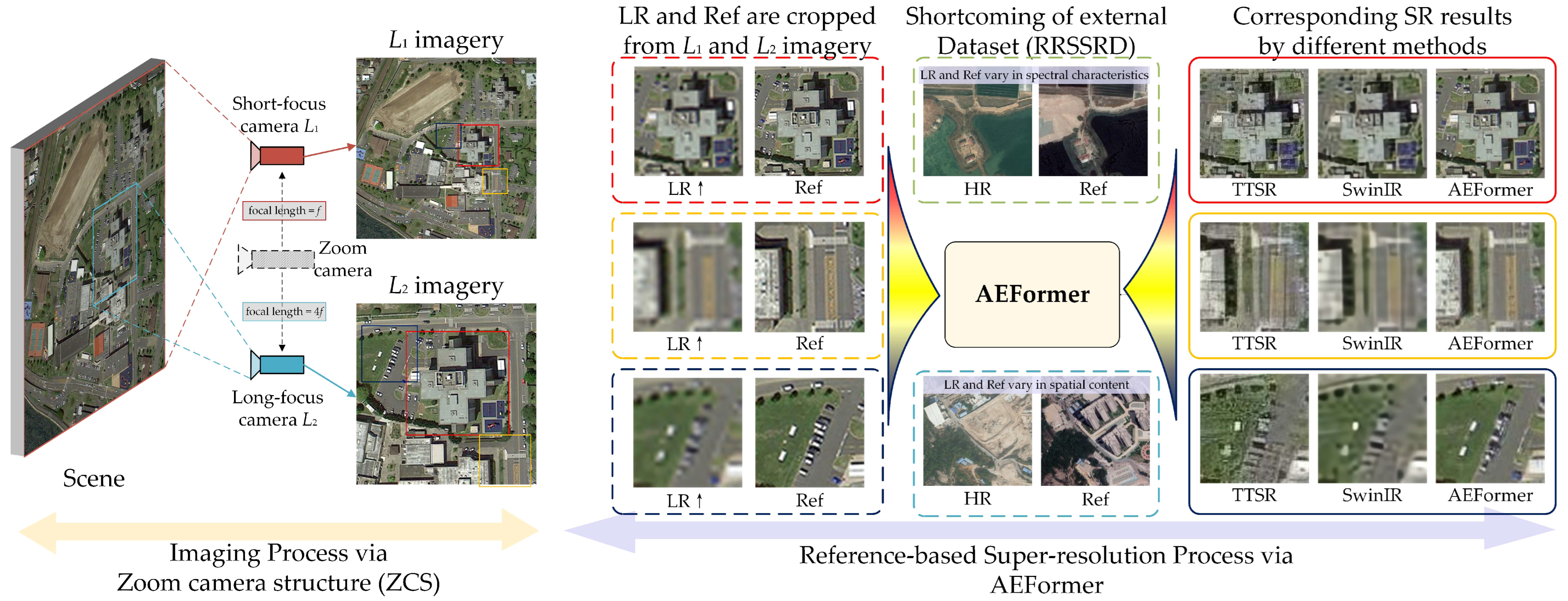
Figure 1. Overall framework of the proposed method follows the process of ‘imaging then super resolution’. Imaging process is based on the proposed ZCS which is composed of a short focus camera L1 and a long focus camera L2. Super-resolution process is based on the proposed AEFormer which adopts LR and Ref as inputs and generates SR as an output. LR and Ref images are cropped from L1 imagery and L2 imagery, denoted in squares of different colors, respectively. ↑ denotes upscale ×4. SR results by TTSR [14], SwinIR [41], and our method are compared.
Remotesensing 15 05409 g001
Figure 2. The working mechanism of ZCS in remote sensing practice. In most cases, to expand the imaging area, short-focus camera L1, which is equipped with wide FOV, is used for wide-field imaging, as shown in position 1, 2, and 3. However, when it is in need for super-resolving ROI in the image captured by L1, a zoom camera switches to long-focus camera L2 which is equipped with narrow FOV, to capture Ref, as shown in position 4. ↑ denotes upscale ×4.
Remotesensing 15 05409 g002
Figure 3. Overview of the proposed AEFormer. In this study, F denotes the feature space while I denotes the image space. Three levels of Ref feature F i R e f are aligned with LR via aligned and enhanced attention and then transferred to the LR feature space through dynamic transfer. For improved model generalization, LR and Ref images are selected from external dataset RRSSRD [11] which vary in spectral characteristics and spatial content. ↑ denotes upscale ×4.
Remotesensing 15 05409 g003
Figure 4. Aligned and enhanced attention. All image branches are transferred to feature space via the learnable texture extractor (LTE). Three branches of the feature map are aligned and concatenated into aligned attention F a t t a l Finally, F a t t a l is concatenated with the swapped feature map F t m p R e f to obtain the final aligned and enhanced attention F a t t A E . Considering the structure of the zoom camera, Ref↓↑ and LR↑ share a common image sampling frequency. In this way, the I R e f branch is added for the alignment process which is novel compared to previous alignment modules [52].
Remotesensing 15 05409 g004
Figure 5. Dynamic transfer module (DTM). Aligned and enhanced attention F a t t A E is transferred into the LR feature space for a better transfer effect with less information loss. Given aligned and enhanced attention F a t t , l e v e l A E and the LR↑ feature map F l e v e l L R of the same level, DTM generates the LR↑ feature map of the next level F l e v e l + 1 L R as the output.
Remotesensing 15 05409 g005
Figure 6. Some examples of HR-Ref pairs within the benchmark dataset RRSSRD [11]. HR images are selected from WorldView-2 (2015) and GF-2 (2018) with a spatial resolution of 0.5 m while Ref images are selected from Google Earth Engine (2019) with consistent or close spatial resolution.
Remotesensing 15 05409 g006
Figure 7. Visual comparison of SR images between the selected methods and ours. Zoom in for better visualization. Bic denotes the bicubic image of LR which is also denoted as LR↑ in the field of super resolution. HR denotes high-resolution imagery which is also known as ground truth (GT).
Remotesensing 15 05409 g007
Figure 8. Improvement percentage (corresponding method compared to bicubic imagery) of each indicator in Table 1. The higher improvement percentage is, the better corresponding method is.
Remotesensing 15 05409 g008
Figure 9. Real-world imagery super resolution based on ZCS. The arrow points to the main differences among compared methods. Zoom in for better visualization.
Remotesensing 15 05409 g009
Figure 10. SR results according to different ZCS configuration. The first row displays different Ref images obtained by different ZCS configuration, while the second row displays corresponding SR results. Given fixed L1 configuration (L1 imaging with f), changes in ZCS include: (a) L2 imaging with f; (b) L2 imaging with 2f; (c) irrelevant imagery; (d) external data (from Google Earth Engine 2023); (e) Real ZCS configuration (L2 imaging with 4f).
Remotesensing 15 05409 g010
Table 1. Average LPIPS, PI, NIQE, FID, IS, PSNR, and SSIM scores of selected SR methods of ×4 factor on different test sets. For LPIPS, PI, NIQE and FID, a lower score indicates a better result whereas for IS, PSNR and SSIM, a higher score indicates a better result. The best results are highlighted in red (first best) and blue (second best).
Test SetMetricsBicubicEDSR
[22]
SPSR
[25]
CrossNet [12]SRNTT [13]TTSR
[14]
TTSR_rec [14]SwinIR [41]AEFormer (Ours)AEFormer
_rec (Ours)
1LPIPS0.36670.16880.17230.28970.20040.19440.23230.23510.10350.1639
PI7.10205.12903.29185.39493.74713.41925.75056.23643.20005.5191
NIQE7.79335.68774.29806.01944.12054.16736.26676.95304.23096.0150
FID126.041389.988075.616090.023589.406189.227197.1016123.056739.104279.7634
IS1.92992.09192.00711.93162.07961.98362.01152.08831.98822.0982
PSNR29.684032.283530.421631.080129.122130.958932.861733.412232.451934.2224
SSIM0.79140.87500.79080.85900.79770.79570.85580.87580.84700.8915
2LPIPS0.39200.27040.21050.30930.23480.21100.24000.26810.13400.1960
PI7.01394.90103.09755.27043.74983.19805.88046.26323.19275.6102
NIQE7.65055.51224.01605.95804.11044.00126.50536.94574.19176.2035
FID127.7582104.133998.8441113.6950115.457299.1046107.9276125.678447.971883.3458
IS2.08222.08362.05431.99802.16432.09332.11412.13762.12002.1272
PSNR29.562131.164629.297731.089527.906329.998132.112632.567931.665933.2675
SSIM0.76380.83190.74460.82950.77270.75430.82750.84060.81190.8615
3LPIPS0.47480.27120.20400.32660.24260.22120.32100.34910.14140.2874
PI7.04935.01032.86305.11903.91613.02135.85686.55962.83145.7783
NIQE7.68045.49213.93245.14934.32543.95016.34197.34283.91686.2950
FID138.0656101.591373.8934106.984980.108475.891799.1774127.083743.279998.4504
IS1.91271.98252.00011.91972.10882.02762.01701.96562.03591.9612
PSNR27.765829.490028.008428.983227.889028.743930.549130.903229.616331.3204
SSIM0.72750.80710.70820.78970.74720.72810.79970.81170.76460.8282
4LPIPS0.37490.28070.24270.32160.25740.23260.24700.28170.15090.2143
PI7.17935.39963.31955.40734.29473.42776.35086.50943.53296.1760
NIQE7.77965.69104.10895.87884.55994.03596.86737.24254.28296.6927
FID123.850998.8013104.6603112.0716112.900599.0680100.5237124.460557.211688.4482
IS2.15702.15632.17532.09942.12252.18602.11722.11402.17872.1158
PSNR30.046531.524629.199630.107729.224730.133832.445032.948731.922833.5955
SSIM0.75930.82330.72310.76900.76870.73940.81840.83100.79620.8496
AverageLPIPS0.40210.24780.20740.31180.23380.21480.26010.28350.13250.2154
PI7.08615.11003.14305.29793.92693.26665.95966.39223.18935.7709
NIQE7.72605.59584.08885.75144.27914.03866.49537.12104.15566.3016
FID128.929098.628688.2535105.693899.468190.8229101.1826125.069846.891987.5020
IS2.02052.07862.05921.98722.11882.07262.06502.07642.08072.0756
PSNR29.264631.115729.231830.315128.535529.958731.992132.458031.414233.1015
SSIM0.76050.83430.74170.81180.77160.75440.82540.83980.80490.8577
Table 2. Evaluation of Real-world imagery SR. Both PI and NIQE are non-reference image quality evaluation metrics. For PI and NIQE, a lower score indicates better. The best results are highlighted in bold.
MethodsData (1)Data (2)
PINIQEPINIQE
SPSR [25]3.5083.30523.01973.1995
SRNTT [13]3.51423.91323.17933.8485
TTSR [14]5.66525.81285.30235.5889
SwinIR [41]6.46446.91576.43447.0353
AEFormer2.88903.53672.96473.6203
Table 3. Evaluation of SR results according to different ZCS configuration. For PI and NIQE, a lower score indicates better. The best results are highlighted in bold.
ZCS ConfigurationData (1)Data (2)
PINIQEPINIQE
Irrelevant image as Ref2.90433.59122.98293.6536
Google Earth as Ref2.99593.77492.88063.5593
Ref with focal length = f3.18773.73402.99603.6807
Ref with focal length = 2f2.91893.58392.98103.6476
Ref with focal length = 4f2.88903.53672.96473.6203
Table 4. Ablation study on the Ref↓↑ branch; aligned and enhanced attention. Ref↓↑ branch denotes the existence of Ref↓↑ in Figure 4 while aligned attention and enhanced attention denotes correspondence in Figure 4. Evaluation metrics are estimated on the first test set from RRSSRD. For LPIPS, a lower score indicates a better result whereas for PSNR and SSIM, a higher score indicates a better result. The best results are highlighted in bold.
ModuleEvaluation Metrics
Ref↓↑ BranchAligned AttentionEnhanced AttentionLPIPSPSNRSSIM
×××0.158030.96930.8171
××0.136231.98330.8392
×0.113932.47020.8396
0.103532.45190.8470
Table 5. Ablation study of transfer module. The first row denotes features concatenation in channel without further operations. The last row denotes the proposed DTM. For LPIPS and PI, a lower score indicates better, whereas for PSNR and SSIM, a higher score indicates better. Evaluation metrics are estimated on the first test set from RRSSRD. The best results are highlighted in bold.
Module within Transfer ModuleEvaluation Metrics
Sigmoid ModuleConvolution ModuleLPIPSPIPSNRSSIM
××0.24956.278032.37980.8320
×0.18966.199332.71640.8426
×0.20986.381732.93540.8371
0.16395.519134.22240.8915
Disclaimer/Publisher’s Note: The statements, opinions and data contained in all publications are solely those of the individual author(s) and contributor(s) and not of MDPI and/or the editor(s). MDPI and/or the editor(s) disclaim responsibility for any injury to people or property resulting from any ideas, methods, instructions or products referred to in the content.