Abstract
Chestnut trees hold a prominent position in China as an economically significant forest species, offering both high economic value and ecological advantages. Identifying the distribution of chestnut forests is of paramount importance for enhancing efficient management practices. Presently, many studies are employing remote sensing imaging methods to monitor tree species. However, in comparison to the common classification of land cover types, the accuracy of tree species identification is relatively lower. This study focuses on accurately mapping the distribution of planted chestnut forests in China, particularly in the Huairou and Miyun regions, which are the main producing areas for Yanshan chestnuts in northeastern Beijing. We utilized the Google Earth Engine (GEE) cloud platform and Sentinel-2 satellite imagery to develop a method based on vegetation phenological features. This method involved identifying three distinct phenological periods of chestnut trees: flowering, fruiting, and dormancy, and extracting relevant spectral, vegetation, and terrain features. With these features, we further established and compared three machine learning algorithms for chestnut species identification: random forest (RF), decision tree (DT), and support vector machine (SVM). Our results indicated that the recognition accuracy of these algorithms ranked in descending order as RF > DT > SVM. We found that combining multiple phenological characteristics significantly improved the accuracy of chestnut forest distribution identification. Using the random forest algorithm and Sentinel-2 phenological features, we achieved an impressive overall accuracy (OA) of 98.78%, a Kappa coefficient of 0.9851, and a user’s accuracy (UA) and producer’s accuracy (PA) of 97.25% and 98.75%, respectively, for chestnut identification. When compared to field surveys and official area statistics, our method exhibited an accuracy rate of 89.59%. The implementation of this method not only offers crucial data support for soil erosion prevention and control studies in Beijing but also serves as a valuable reference for future research endeavors in this field.
1. Introduction
Chestnut (Castanea mollissima Blume) is a deciduous tree belonging to Castanea of Fagaceae, a species that is originally from China. It is a famous nut tree and one of the earliest fruit trees domesticated and utilized in the country [1], with high economic value and ecological benefits [2]. China’s chestnut is of excellent quality and rich in nutrients, and its existing cultivation area and annual output rank first in the world [3,4]. Chestnut is mostly distributed in mountainous and hilly areas, and the chestnut industry has been leading the market in the area, increasing agricultural efficiency and farmers’ income in the mountainous regions of Beijing. Chestnut tree species have also demonstrated the effect of increasing surface coverage, improving soil, and reducing soil erosion in many soil and water conservation projects [4]. However, the planting density of the chestnut economic forest is usually low, and carrying out weeding and other operations before the harvest of the fruit easily leads to long-term exposure and loosening of the undergrowth land, resulting in the degradation of vegetation and death of chestnut trees [4,5,6]. Therefore, it is of great significance to establish an automatic remote sensing identification method for chestnut forest distribution to improve the efficient management of economic forests and help maintain China’s sustainable economic and social development.
Compared with traditional field monitoring, remote sensing image identification of tree species distribution has the advantages of large spatial range and flexible time-frequency, which can cover forest areas that are difficult for human beings to enter. Remote sensing imaging methods have been widely used in tree species monitoring [7,8,9]. Optical remote sensing data are the mainstream data currently used in the classification of ground objects, and they can be divided into three categories according to spatial resolution: medium-resolution data (250–1000 m), high-resolution data (less than 10 m) and medium- and high-resolution data (10–250 m). For example, moderate resolution imaging spectrometer (MODIS) data have been widely used in regional-scale mapping, and the producer’s accuracy is usually low [10,11,12] due to the serious mixed pixel effect. The details of high-resolution data are clearer, but the limited space–time coverage and high cost make it difficult to realize large-scale applications [13,14,15,16]. Among the medium- and high-resolution data, Sentinel-2 series images have high spatial resolution, rich spectral information, many selectable phases, and free access, which can support accurate and wide spatial coverage and long-term plant monitoring. Many studies have reported the successful implementation of classification mapping [17,18] with Sentinel-2 data on a regional scale. Based on Sentinel-2A multi-temporal images, Li et al. used an RF algorithm to identify and classify tree species in Dagujia Forest Farm [19]. Gu et al. made full use of the rich information of Sentinel-2 data in the red edge band and used a variety of vegetation indices to combine them into a time series for crop classification [20]. Jiang et al. put forward a remote sensing comprehensive classification scheme [21] that is suitable for coniferous forests in the Tianshan mountains using a comprehensive analysis of the shadow distribution temporal characteristics, classification characteristics, and classifier selection based on two Sentinel-2 images with great differences in solar altitude and azimuth. However, a single-phase image can only extract limited spectral characteristics of vegetation, some of which are similar between different forests.
More and more researchers have begun to explore multiple-phase images to derive high-resolution and high-precision species mapping [22,23]. In our study, compared with the common classification of land cover types, it became more challenging to identify tree species. It is not enough to only use the differences in spectral and spatial texture in a single phase between the target tree species and other ground objects. Hence, we try to fully explore the differences in seasonal curves and phenological characteristics from multiple-phase images to better understand this distinction.
Regarding the requirement of large-scale and long-time series of remote sensing images in vegetation phenology analysis, the GEE (Google Earth Engine) Cloud Platform is considered to be a great software for this matter [24,25]. It stores publicly available remote sensing image data such as Sentinel/Landsat in Google’s disk array so that GEE users can conveniently extract, call, and analyze massive remote sensing big data resources [26,27]. Yang et al. automatically generated winter wheat training samples with the temporal and spectral characteristics of Sentinel-2 images on the GEE platform and used the OCSVM classification method to draw the winter wheat planting area map of Jiangsu Province in China in different seasons [28]. Tian et al. proposed a pixel-based phenological feature composite method (Ppf-CM) to reduce the spatial variability of phenology but also enhance the spectral separation between Spartina alterniflora and native species by superimposing two unique phenological features [29].Ni developed enhanced Ppf-CM (Eppf-CM) in the GEE platform to make full use of several representative phenological stages of rice and obtained one of the rice maps with the highest spatial resolution of 10 m on the regional scale in Northeast China [30]. Currently, just a few studies in the field are focused on remote sensing extraction of chestnut forests. Some domestic researchers have relied on high-resolution WorldView imagery to identify the distribution of chestnut trees scattered within agricultural and urban environments [14,15] and used the optimal temporal phase and classification features for chestnut forest extraction by integrating MODIS and Landsat data [21]. However, there is still a lack of research concerning the utilization of Sentinel-2 imagery’s advantages for extracting vegetation phenology features to identify chestnut forests.
Hence, this study leverages the high temporal and spatial resolution of Sentinel-2 images to extract multiple classification features, including vegetation phenological characteristics. Consequently, we employed the Google Earth Engine (GEE) platform to establish and optimize a machine learning model, aiming to develop a high-precision method for automatically identifying planted chestnut forests and generating accurate distribution maps in northeastern Beijing. The implementation of this method not only offers crucial data support for soil erosion prevention and control studies in Beijing but also serves as a valuable reference for future research endeavors in this field.
2. Materials and Methods
2.1. Study Area
Huairou and Miyun districts in Beijing are selected as the study area (Figure 1). Situated within the Yanshan Mountains, these districts constitute the primary chestnut-producing region, and the majority of chestnut forests are artificially planted. Within the geographical coordinates of 40°13′~41°4′N and 116°17′~117°30′E. The area is located at the juncture of the Yanshan mountainous region and the North China Plain in the Northeast of Beijing. Its territory is low in the south and high in the north, with an altitude of 34 m to 1705 m. It has a warm temperate semi-humid climate, with an average annual temperature of 9~13 °C and an average annual precipitation of 600~700 mm, mainly in June and August. Huairou District has a total area of 2123 km2, and more than 89% of the land in the area is hilly and mountainous, which is suitable for planting chestnuts. Therefore, Huairou District has a large planting area and is known as the “hometown of chestnuts in China”. Currently, its chestnut output and export account for 70% of the city. Miyun District in Beijing, with a total area of 2230 km2, is the largest district in the capital. Driven by economic interests and other factors, chestnut has also become the most widely distributed and planted economic forest species in Miyun District, mainly distributed in the shallow mountainous areas of towns and villages such as Dachengzi, Beizhuang, Fengjiayu, and Bulaotun in the upper reaches of the reservoir, generally concentrated and contiguous, with less sporadic distribution. The most suitable areas for chestnut growth in Huairou North and South Gully include Jiuduhe Town, Bohai Town, and Yugou Village in Qiaozi Town.
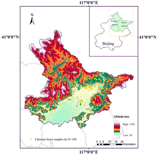
Figure 1.
Geographical location of the study area.
2.2. Data Source and Processing
2.2.1. Sentinel-2 Time Series Images
The Sentinel-2 data used in this research were obtained from the GEE platform (https://code.earthengine.google.com (accessed on 10 January 2022)). The dataset includes 12 images, collected monthly from June 2020 to June 2021. Spectral bands with 10 m ground resolution were selected to enable high-frequency, continuous, and dynamic monitoring of the Earth’s surface [16]. To improve the quality and usability of the data, we performed atmospheric correction, cloud removal, resampling, and other preprocessing steps to mitigate the effects of atmospheric and illumination factors on ground object reflection.
2.2.2. DEM Data
It is understood that the planting altitude of chestnuts in mountainous areas is generally less than 400 m, and chestnut trees prefer light, so it is best to plant them on sunny slopes, and all slopes within 45 degrees can be planted. Hence, it is concluded that the distribution of chestnut forests has a great relationship with topographic factors. To analyze the topographic factors, we utilized DEM (digital elevation model) data from the 2011 Advanced Land Observation Satellite (ALOS) phased array L-band SAR. The data, which had a spatial resolution of 12.5 m, were obtained from the public resource website https://earthdata.nasa.gov/ (accessed on 10 January 2022).
To calculate the slope and aspect features, the DEM data were uploaded onto the GEE platform. Bilinear interpolation functions were then applied on the GEE platform to resample the ALOS DEM data to a resolution of 10 m. This was carried out to ensure consistency between its resolution and that of the remote sensing data.
2.2.3. Field Survey Sample Data
In order to fully understand the types of ground objects in the study area and grasp the spatial location information of typical samples, investigators conducted field investigations in Huairou and Miyun District of Beijing in the summer of 2021. The latitude and longitude coordinates of representative plots were measured with a hand-held GPS and the corresponding land types and vegetation types were recorded. The land cover in the study area is divided into six categories: cultivated land, chestnut forest land, deciduous forest land (including shrub and deciduous vegetation, accounting for a small proportion), evergreen forest land, water area, and construction land. A total of 41,236 pixels of Sentinel-2 images in 440 regions of interest were selected as the sample data for machine learning, and the training and verification samples were randomly divided according to the ratio of 7:3 (see Table 1).

Table 1.
Training samples and verification samples.
2.2.4. Accuracy Verification Data
To verify the spatial distribution classification accuracy of chestnut forests, deciduous forests, evergreen forests, cultivated land, water area, and construction land, besides verification samples obtained from the ground investigation, we also collected the official statistical data of the total area of chestnut forests in the study area in 2020, the forest resources survey data, and cultivated land statistical data. With the help of 10 m global land use data [31] provided by ESRI in 2020 (https://www.arcgis.com/ (accessed on 10 January 2022)), these data were used to verify the classification accuracy.
2.3. Methods
2.3.1. Feature Selection and Construction
(1) Terrain Characteristics
Terrain factors such as elevation, slope, and aspect can affect plants under the comprehensive action of light, temperature, rainfall, wind speed, soil texture, and other elements, thus causing changes in the ecological relationship between plants and the environment and affecting the planting area of chestnut. Therefore, we selected elevation, slope, and aspect to classify the ground objects, and the factors obtained from the DEM data of Miyun District and Huairou District in Beijing are normalized to be the terrain characteristics.
(2) Spectral Characteristics
Spectral feature is the most direct and important interpretation element in remote sensing image recognition, which shows different pixel gray values in remote sensing images, so the difference between pixel gray values of various ground objects can be used as the basis for ground object recognition. In this study, Sentinel-2A satellite images with 10 m and 20 m spatial resolution bands are selected, including blue band (B2), green band (B3), red band (B4), red edge bands (B5, B6, B7, B8a), near-infrared band (B8), and shortwave infrared bands (B11, B12), totaling 10 spectral characteristics (see Table 2).
Table 2.
Selected band parameters of Sentinel-2A satellite.
(3) Vegetation Characteristics
In the traditional sense, the band reflectivity is usually used as the remote sensing distinguishing feature of designated objects. However, in reality, not all working bands are effective enough for chestnut recognition. Thus, we considered adding some extended features, such as multiple vegetation indices, to participate in the extraction of chestnut planting areas and evaluate the performance of each extended feature in chestnut recognition. Sentinel-2 images contain three visible bands and two shortwave infrared bands, which are very effective for monitoring vegetation health information. According to the vegetation-sensitive bands unique to Sentinel-2 data, 10 targeted vegetation indices were selected for classification. The specific index calculation is shown below in Table 3.
Table 3.
Vegetation indices selected for this study.
(4) Phenological Characteristics
The NDVI vegetation index of the corresponding position used in this study was obtained from Sentinel-2 images, and the NDVI time series curves of six typical ground objects in the study area were obtained through drawing. Then, a Savitzky–Golay (SG) filter [42] was implemented to smooth the contour and facilitate the analysis of the time series variation characteristics of NDVI and help determine the key phenological period of chestnut. The smoothing window parameter of SG was set to 10, and the degree of smoothing polynomial was set to 2.
The phenological characteristics of chestnut trees were outlined by analyzing and selecting the significant spectral characteristics and vegetation index characteristics of different key phenological periods. First, the median composite image containing abundant phenological information was generated for each cloudless pixel in all Sentinel-2 images in different phenological periods. With that, we could obtain the reflectance curves of spectral bands in three phenological periods of chestnut trees. The combination of phenological periods and spectral bands is selected according to the difference between the reflectance of chestnut woodland in different spectral bands and other land types. Then, according to the Sentinel-2 images, the vegetation indices in different phenological periods were extracted, and the distribution characteristics of the vegetation indices in different phenological periods were analyzed by making box charts. Finally, we selected the vegetation indices with a large scale in different phenological periods and constructed the phenological characteristics.
2.3.2. Machine Learning Classification Method
According to various classification feature combinations of the input phenological features, three machine learning algorithms including SVM (support vector machine), DT (decision tree), and RF (random forest) algorithms were used to identify and compare land types. The machine learning algorithm with the best fitting effect was selected to extract chestnut forest. In the process of classification using three machine learning methods, 70% of the sample data were selected as training samples to train the model, and 30% of the samples were used as test samples to evaluate the model’s accuracy.
(1) SVM Algorithm
SVM is a kind of generalized linear classifier that classifies data using supervised learning. Its decision boundary is the hyperplane with the maximum side distance for learning samples [43]. In this study, we implemented the SVM algorithm by calling the ee.Classifier.libsvm () function on the GEE platform, in which the input of the key parameter kernel function type determines the classification performance of SVM. The kernel functions of the algorithm include the linear kernel function (SVM-L), polynomial kernel function (SVM-P), Gaussian radial basis kernel function (SVM-R), and S kernel function (SVM-S). SVM-L was selected to carry out the remote sensing identification of chestnut forest land.
(2) DT Algorithm
The DT classification algorithm is a nonparametric supervised classification method that classifies remote sensing image pixels according to the segmentation threshold [44]. At present, it includes three common types: ID3, C4.5, and CART. The CART algorithm was used to perform the surface feature classification in the study area and we used the ee.Classifier.smileCart() function of the GEE platform to perform its training. The two key parameters were the maximum number of leaf nodes and the minimum number of samples contained in each leaf node. The parameter values used in this study were set to their default settings for the method.
(3) RF Algorithm
RF is a classifier that consists of multiple decision trees, with the final output class being determined by the mode of the classes output by individual trees. Using this algorithm and combining the decisions of multiple trees, it is possible to enhance the accuracy and stability of classification [45]. Therefore, the RF algorithm has the advantages of avoiding overfitting and high algorithm precision. We used the ee.classifier.smileRandomForest() function on the GEE platform to implement it and set two key parameters: the number of decision trees T and the number of node splitting features M, which has an important impact on the model training effect. Generally, increasing T can effectively reduce the generalization error of the model, but it can also reduce the computational efficiency. M is the decisive factor in the classification performance of a single decision tree and has an impact on the correlation between trees.
First, we optimized two key parameters and then input sample data to establish an RF model for classification. In the RF algorithm, the upper limit of parameter T is generally set to 1000, and M is the quadratic root of the number of features by default (taking a root of 66 and the result is about 8). Therefore, when constructing the RF algorithm, we set the value range of parameter T as 1–1000 and parameter M as 2, 4, 6, 8, and 10. Based on the training samples, the random forest ground object classification under all parameter combinations is carried out and the out-of-pocket error is used as the evaluation basis. The operation efficiency and stability of the algorithm were comprehensively considered to finally determine the optimal values of the parameters T and M.
2.3.3. Accuracy Evaluation
In order to test the stability and accuracy of the model, the samples were divided according to the proportion of 7:3 [46,47]. We used 70% samples as the training set for establishing the model, and 30% samples were used as the test set for evaluating the model. We also set four commonly used evaluation indicators, namely, the producer’s accuracy (PA), user’s accuracy (UA), overall accuracy (OA), and Kappa coefficient, to evaluate the accuracy of model classification. PA is the ratio between the correct prediction of a certain category and the actual number of such categories, reflecting the degree of missing points of a certain category; UA is the ratio of a certain type of wrong prediction to the actual quantity, reflecting the degree of wrong classification of a certain type; OA is the proportion of correctly predicted samples to all samples, reflecting the overall accuracy of algorithm classification; and Kappa is a measure of the consistency between the predicted value and the actual value. Kappa is often used to assess the reliability of classification accuracy, with the value ranging from −1 to 1. A value of 0.75–1 means very good consistency, 0.4–0.75 means good consistency, 0–0.4 means poor consistency, and negative values mean less consistency than contingency.
The accuracy evaluation index is calculated by constructing the confusion matrix, and the total number of each column of the confusion matrix represents the number of data predicted for this category. Furthermore, each row represents the real category of data, and the total number of data in each row represents the number of data instances of that category. The numerical values in each column are the numbers of real data predicted as such. The calculation formulas of PA, UA, OA, and Kappa coefficients based on the confusion matrix are as follows [48]:
where is the total number of pixels, is the number of categories classified, is the number of pixels on the diagonal of the confusion matrix, and and are the total number of pixels in row and column , respectively.
3. Results
3.1. Phenological Characteristic Construction
Generally, the growth period of Chinese chestnut (that is, from germination to defoliation) is 245 days. It usually sprouts at the end of the first ten days, produces leaves in the middle ten days, and produces new shoots in the last ten days of March. Male flowers are exposed and gradually elongate in the first ten days, and female flowers appear in the second ten days of April. The flowers bloom in May and fade in early June, and the shell begins to expand and harden and their seed growth period is from July to August. The nuts mature in early September, and leaves fall in early November and then enter dormancy. The NDVI time series curve (Figure 2) obtained in this study reflects the growth and development of Chinese chestnut in a year, as well as significant differences with other surface feature types. In the whole time series, the NDVI value of evergreen forest is relatively high, and the NDVI value of water bodies is mostly negative. Chinese chestnut has a relatively similar NDVI value to that of cultivated land and deciduous forest land. However, in the early and late growth stages, we observed a significantly different change compared to other ground objects.

Figure 2.
Time series change curve of NDVI in the study area.
Three key phenological periods with high discrimination were determined by analyzing the NDVI time series curve: ① the flowering period of Chinese chestnut (1 April to 31 June): During this time, the NDVI curve of cultivated land, Chinese chestnut forest, and deciduous forest exhibit distinct variations due to their different flowering characteristics. ② Chinese chestnut fruiting period (15 August to 31 October): At this time, the Chinese chestnut forest and deciduous forest are relatively dense. Most vegetation in the cultivated land has been picked in preparation for the Chinese chestnut harvest, but the deciduous and evergreen forests still have strong vegetation growth. ③ Dormancy period of Chinese chestnut (1 December to the end of February): The NDVI value of evergreen forest is significantly higher than that of other ground objects during this period, owing to its distinctive vegetation cover.
The reflectance curves of spectral bands of three phenological periods of Chinese chestnut were generated based on the Sentinel-2 median composite images of different phenological periods of flowering, fruiting, and dormancy of Chinese chestnut (Figure 3). The reflectance of the red band (Band 4), the nearinfrared band (Band 8), and the shortwave infrared band 2 (Band 12) of different land cover types during the flowering period of Castanea mollissima are highly distinguishable. The reflectance of the red band (Band 4) is mainly different in chestnut forest land, deciduous forest land, and cultivated land. The near-infrared band (Band 8) plays a major role in distinguishing non-vegetation areas, and the reflectance of the shortwave infrared band 2 (Band 12) is more distinguishable for six surface feature types. However, the reflectivity of other bands in the flowering period of Chinese chestnut has cross convergence, and there is no obvious difference among various ground features. The blue band (Band 2), green band (Band 3), and narrow and red edge band 4 (Band 8A) of the chestnut fruit stage are relatively distinct, which can be used as the classification spectral characteristics of the fruit stage. The reflectance of the blue and green bands in cultivated and construction land is higher than that of other surface features, while the reflectance of the red edge band 4 (Band 8A) in chestnut forest land is significantly higher than that of other land covers. In addition, during the dormancy period of Chinese chestnut, the red edge band 1 (Band 5), red edge band 2 (Band 6), red edge band 3 (Band 7), and shortwave infrared band 1 (Band 11) reflectance of the ground objects are significantly different.
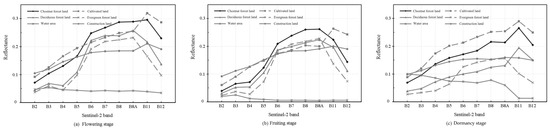
Figure 3.
Reflectance curve of chestnut forest land and other surface feature types at (a) flowering stage, (b) fruit stage, and (c) dormancy stage.
We extracted the vegetation index in different phenological periods and outlined the box graph according to the Sentinel-2 images. Based on the median, mean, quarter, and three-quarter values of the box graph, we analyzed the distribution characteristics of the vegetation index in different phenological periods and selected the optimal vegetation index characteristics under different phenological periods to construct the phenological characteristics. The analysis results are shown in Figure 4. The distribution characteristics of the EVI, NDVI, PSRI, and MTCI vegetation indices in the flowering period of Chinese chestnut are quite different from those of other land types. Furthermore, the distribution characteristics of the MNDWI, WDRVI, and REP vegetation indices in the fruiting period are also different from those of other land types. There are also considerable differences in the distribution characteristics of the GNDVI, NDBI, and SAVI vegetation indices in the dormancy period of other land types.

Figure 4.
Box plot of vegetation index in different phenological periods at sample points of each category, including median, mean, quarter, three-quarters, and outliers.
Based on the above analysis of spectral band reflectance and vegetation index values of each phenological period, we listed 20 characteristic factor combinations of three chestnut phenological periods to outline the phenological characteristics. The flowering period corresponded to seven key indicators, the fruiting period corresponded to six key indicators, and the dormancy period corresponded to seven key indicators, as shown in Table 4.
Table 4.
Phenological combinations and their corresponding indicators.
3.2. Comparison of Identification Methods of Chestnut Forest
This study mainly involved the identification and comparative analysis of chestnut forests using various feature combinations and machine learning methods. Initially, four feature combinations were created based on whether phenological features and topographical features were considered, as outlined in Table 5. Subsequently, a total of twelve methods were formulated by combining these feature combinations with three different machine learning models, i.e., SVM, DT, and RF. These twelve methods were then applied to identify land cover in the Miyun and Huairou districts using Sentinel-2 images, and the results are depicted in Figure 5 for reference.
Table 5.
Characteristic combinations and their corresponding indicators.
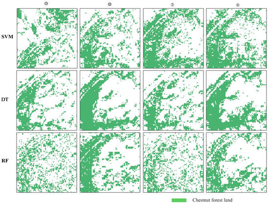
Figure 5.
Comparison of results of different classifiers and different methods. Different rows represent three machine learning algorithms, and different columns represent different recognition methods. ① Representative characteristic factors include spectral characteristics and vegetation characteristics. ② Representative characteristic factors include spectral characteristics, vegetation characteristics and phenological characteristics. ③ Representative characteristic factors include spectral characteristics, vegetation characteristics, and terrain characteristics. ④ Representative characteristic factors include spectral characteristics, vegetation characteristics, phenological characteristics, and phenological characteristics.
The accuracy results of each classification method (see Figure 6) show that the method (i.e., the fourth combination of eigenvalues) based on spectral and vegetation characteristics considering topographic and phenological features has the best effect. In particular, considering phenological characteristics is evidently better than not considering phenological characteristics in these recognition methods. Compared with the third combination of eigenvalues, the overall accuracy and Kappa coefficient of the fourth combination of eigenvalues are improved by 4.1%, 0.73%, 1.62%, and 0.0541, 0.0096, and 0.0198, corresponding to the results of the SVM, DT, and RF algorithms, respectively. Among the three machine learning algorithms, the RF algorithm has the highest accuracy. Under the fourth eigenvalue combination, the overall accuracy and Kappa coefficient are increased to 98.52% and 0.9820, and the user’s accuracy and producer’s accuracy of chestnut forest land are increased to 97.25% and 99.46%, respectively.

Figure 6.
Comparison of identification methods.
Overall, the RF algorithm with spectral, vegetation, phenological, and terrain characteristics had the best performance, achieving the highest evaluation accuracy. Therefore, we selected this method to identify Chinese chestnut forests in the Miyun and Huairou Districts.
3.3. Identification Result and Accuracy Evaluation
The land cover map and the distribution map of Chinese chestnut forest land in the Huairou and Miyun areas of Beijing were obtained through the RF algorithm considering phenological and topographic characteristics. This map has a resolution of 10 m. The map is shown in Figure 7.

Figure 7.
Land cover type map.
By evaluating the identification results using field survey sample data, the confusion matrix for the RF model yielded the following values: TP (true positive) = 3664, FP (false positive) = 104, TN (true negative) = 8501, and FN (false negative) = 46. The overall accuracy of classification mapping is higher than 98%, and the Kappa coefficient is above 0.9. In the vegetated areas (chestnut forest, cultivated land, deciduous forest, and evergreen forest), the accuracy reaches 92.43%. Chestnut is wrongly classified into different tree species, mainly pear, walnut, hawthorn, and other fruit trees, as well as some terraced fields and cultivated land. In the non-vegetated area (including water area and construction land), the accuracy is nearly 100%.
Compared with the chestnut forest land area stated in the official statistical data (see Table 6), the extracted area of chestnut in this study is 320.85 km2, which accounts for 89.59% of the official statistical data’s 357.17 km2. The distribution of chestnut in Huairou and Miyun districts is 47.56% and 52.44%, respectively, closely resembling the statistical data of 41.06% and 58.94%.
Table 6.
Comparison of chestnut area and percentage in the distribution map with official statistics in 2020.
4. Discussion
Previous studies have demonstrated that the accuracy [21] of Chinese chestnut forest identification can be effectively improved by utilizing medium- and high-resolution images. Our analysis results based on Sentinel-2 images, align with this finding and further highlight the advantages of classification mapping with Sentinel-2 images. These advantages include high spatial resolution, abundant spectral information, numerous selectable phases, and free accessibility. However, better recognition results would be achieved by separately identifying chestnut forests in flat terrain and mountainous areas.
Relying on the traditional consideration of images’ spectral and vegetation characteristics, we took into account the differences in the characteristics of vegetation in the process of growth and development. The introduction of vegetation phenological and topographic features in this study improved the quality of the chestnut forest distribution recognition map and guaranteed its recognition accuracy. It is consistent with the studies by Li et al. [22] and Lei et al. [23], who highlighted the importance of incorporating phenological characteristics and topographic features to enhance the classification accuracy in land cover mapping.
In order to avoid mistakes when classifying Chinese chestnut forests, early research introduced other auxiliary data to reduce the similarity and proved that machine learning algorithms are effective in improving the accuracy of ground object classification [49]. Following the research hotspot in the field of machine learning, we selected three machine learning algorithms to identify the distribution of chestnut forests in Miyun District and Huairou District (Beijing). We found that the RF algorithm is significantly better than the SVM algorithm and the DT algorithm in terms of the producer’s accuracy, user’s accuracy, overall accuracy, and Kappa coefficient results. However, there were still some omissions or classification errors when the RF algorithm was selected and used in this study. We could identify some noise points in the classification results of chestnut forest land, so there is still room for improvement through improving the RF methods. For example, we could consider the interaction between feature indicators to enhance the accuracy.
Overall, although significant progress has been made through the integration of vegetation phenological characteristics and the RF algorithm classification, there are still certain limitations in this study. First, we did not separate the images into flat and mountainous areas for classification, which could potentially impact the accuracy of identification. Second, the inclusion of texture characteristics in image extraction for classification was not considered, thereby potentially limiting the performance improvement. Last, the interaction between feature indicators in the machine learning models was not taken into account.
5. Conclusions
This study focused on the vegetation phenological characteristics of the Yanshan Mountains in the northeast of Beijing and proposed a new method to identify the distribution of chestnut forest based on the Sentinel-2 time series remote sensing images on the GEE cloud platform. First, three key phenological periods were determined for chestnut forest extraction based on Sentinel-2’s high-temporal-resolution observations. Then, using the high-resolution spectral band features and vegetation index features in these three key phenological periods, supplemented with DEM data, we achieved the extraction of chestnut forest data based on the machine learning algorithm. The results showed that: ① High-temporal-resolution Sentinel-2 imagery possesses unique vegetation-sensitive bands, making it well-suited for vegetation identification studies. ② The phenological characteristics of chestnut forests in the area exhibit high distinguishability from other land cover types, and the method for constructing phenological features can enhance the accuracy of chestnut forest identification. ③ Compared to the other two machine learning methods, RF classification performs the best, yielding the highest accuracy in chestnut forest data extraction.
Author Contributions
Conceptualization, J.W.; methodology, N.X., H.C., R.L., H.S. and S.D.; formal analysis, N.X., H.C., R.L., H.S. and S.D.; investigation, N.X., H.C., R.L., H.S. and S.D.; writing—original draft preparation, N.X.; writing—review and editing, N.X., H.C., R.L., H.S., S.D. and J.W.; visualization, N.X., H.C., R.L., H.S., S.D. and J.W.; supervision, J.W.; funding acquisition, J.W. and N.X. All authors have read and agreed to the published version of the manuscript.
Funding
This research was funded by the National Natural Science Foundation of China (grant numbers 42330507, 42101473, 42071342) and the Beijing Natural Science Foundation (grant number 8222052).
Data Availability Statement
Data are contained within the article.
Acknowledgments
We are grateful to the teachers of the Beijing Forestry University and the staff of Beijing City Management Municipal Institute and PIESAT Information Technology Co., Ltd.
Conflicts of Interest
Authors Hailong Chen, Ruiping Li, Huimin Su, Shouzheng Dai were employed by the company PIESAT Information Technology Co., Ltd. The remaining authors declare that the research was conducted in the absence of any commercial or financial relationships that could be construed as a potential conflict of interest.
References
- Han, Y.; Xu, L.; Zhou, J. Current situation and trends of Chinese chestnut industry and market development. China Fruits 2021, 4, 83–88. [Google Scholar]
- Chen, J.; Wei, X.; Liu, Y.; Min, Q.; Liu, R.; Zhang, W.; Guo, C. Extraction of chestnut forest distribution based on multitemporal remote sensing observations. Remote Sens. Technol. Appl. 2020, 35, 1226–1236. [Google Scholar]
- Su, S.; Lin, L.; Deng, Y.; Lei, H. Synthetic evaluation of chestnut cultivar groups in north China. Nonwood For. Res. 2009, 27, 20–27. [Google Scholar]
- Liu, X.; Liu, F.; Zhang, J. Analysis on the layout and prospects of chestnut industry in the Beijing Tianjin Hebei region. China Fruits 2022, 2, 99–102. [Google Scholar]
- Tang, X.; Yuan, Y.; Zhang, X.; Zhang, J. Distribution and environmental factors of Castanea mollissima in soil and water loss areas in China. Bull. Soil Water Conserv. 2021, 41, 345–352. [Google Scholar]
- Wang, S.; Wang, F.; Li, Y.; Yang, X. Preliminary study on the prevention and control of soil and water loss under the chestnut forest in miyun district. Soil Water Conserv. China 2020, 6, 64–66. [Google Scholar]
- Wei, J.; Mao, X.; Fang, B.; Bao, X.; Xu, Z. Submeter remote sensing image recognition of trees based on Landsat 8 OLI support. J. Beijing For. Univ. 2016, 38, 23–33. [Google Scholar]
- Fu, F.; Wang, X.; Wang, J.; Wang, N.; Tong, J. Tree species and age groups classification based on GF-2 image. Remote Sens. Land Resour. 2019, 31, 118–124. [Google Scholar]
- Wang, C.; Li, B.; Zhu, R.; Chang, S. Study on tree species identification by combining Sentinel-1 and JL101A images. For. Eng. 2020, 36, 40–48. [Google Scholar]
- Dong, J.; Xiao, X.; Sheldon, S.; Biradar, C.; Xie, G. Mapping tropical forests and rubber plantations in complex landscapes by integrating PALSAR and MODIS imagery. ISPRS J. Photogramm. Remote Sens. 2012, 74, 20–33. [Google Scholar] [CrossRef]
- Cao, Y.; Chen, E.; Li, S. Estimation of provincial spatial distribution information of forest tree species (group) composition using multi-sources data. Sci. Silvae Sin. 2016, 52, 18–29. [Google Scholar]
- Yu, X.; Zhuang, D. Monitoring forest phenophases of northeast China based on Modis NDVI data. Resour. Sci. 2006, 28, 111–117. [Google Scholar]
- Zhang, Z.; Zhang, Q.; Qiu, X.; Peng, D. Temporal stage and method selection of tree species classification based on GF-2 remote sensing image. Chin. J. Appl. Ecol. 2019, 30, 4059–4070. [Google Scholar]
- Li, D.; Ke, Y.; Gong, H.; Li, X.; Deng, Z. Urban tree species classification with machine learning classifier using worldview-2 imagery. Geogr. Geo-Inf. Sci. 2016, 32, 84–89+127. [Google Scholar]
- Verlič, A.; Đurić, N.; Kokalj, Ž.; Marsetič, A.; Simončič, P.; Oštir, K. Tree species classification using WorldView-2 satellite images and laser scanning data in a natural urban forest. Šumarski List. 2014, 138, 477–488. [Google Scholar]
- Marchetti, F.; Arbelo, M.; Moreno-Ruíz, J.A.; Hernández-Leal, P.A.; Alonso-Benito, A. Multitemporal WorldView satellites imagery for mapping chestnut trees. Conference on Remote Sensing for Agriculture, Ecosystems, and Hydrology XIX. Int. Soc. Opt. Photonics 2017, 10421, 104211Q. [Google Scholar]
- Zhang, D.; Yang, Y.; Huang, L. Extraction of soybean planting areas combining Sentinel-2 images and optimized feature model. Trans. Chin. Soc. Agric. Eng. 2021, 37, 110–119. [Google Scholar]
- Zhu, M.; Zhang, L.; Wang, N.; Lin, Y.; Zhang, L.; Wang, S.; Liu, H. Comparative study on UNVI vegetation index and performance based on Sentinel-2. Remote Sens. Technol. Appl. 2021, 36, 936–947. [Google Scholar]
- Li, Y.; Li, C.; Liu, S.; Ma, T.; Wu, M. Tree species recognition with sentinel-2a multitemporal remote sensing image. J. Northeast. For. Univ. 2021, 49, 44–47, 51. [Google Scholar]
- Gu, X.; Zhang, Y.; Sang, H.; Zhai, L.; Li, S. Research on crop classification method based on sentinel-2 time series combined vegetation index. Remote Sens. Technol. Appl. 2020, 35, 702–711. [Google Scholar]
- Jiang, J.; Zhu, W.; Qiao, K.; Jiang, Y. An identification method for mountains coniferous in Tianshan with sentinel-2 data. Remote Sens. Technol. Appl. 2021, 36, 847–856. [Google Scholar]
- Li, F.; Ren, J.; Wu, S.; Zhang, N.; Zhao, H. Effects of NDVI time series similarity on the mapping accuracy controlled by the total planting area of winter wheat. Trans. Chin. Soc. Agric. Eng. 2021, 37, 127–139. [Google Scholar]
- Lei, G.; Li, A.; Bian, J.; Zhang, Z.; Zhang, W.; Wu, B. An practical method for automatically identifying the evergreen and deciduous characteristic of forests at mountainous areas: A case study in Mt. Gongga Region. Acta Ecol. Sin. 2014, 34, 7210–7221. [Google Scholar]
- Wang, X.; Tian, J.; Li, X.; Wang, L.; Gong, H.; Chen, B.; Li, X.; Guo, J. Benefits of Google Earth Engine in remote sensing. Natl. Remote Sens. Bull. 2022, 26, 299–309. [Google Scholar] [CrossRef]
- Li, W.; Tian, J.; Ma, Q.; Jin, X.; Yang, Z.; Yang, P. Dynamic monitoring of loess terraces based on Google Earth Engine and machine learning. J. Zhejiang AF Univ. 2021, 38, 730–736. [Google Scholar]
- Chen, B.; Xiao, X.; Li, X.; Pan, L.; Doughty, R.; Ma, J.; Dong, J.; Qin, Y.; Zhao, B.; Wu, Z.; et al. A mangrove forest map of China in 2015: Analysis of time series Landsat 7/8 and Sentinel-1A imagery in Google Earth Engine cloud computing platform. ISPRS J. Photogramm. Remote Sens. 2017, 131, 104–120. [Google Scholar] [CrossRef]
- Ghorbanian, A.; Kakooei, M.; Amani, M.; Mahdavi, S.; Mohammadzadeh, A.; Hasanlou, M. Improved land cover map of Iran using Sentinel imagery within Google Earth Engine and a novel automatic workflow for land cover classification using migrated training samples. ISPRS J. Photogramm. Remote Sens. 2020, 167, 276–288. [Google Scholar] [CrossRef]
- Yang, G.; Yu, W.; Yao, X.; Zheng, H.; Cao, Q.; Zhu, Y.; Cao, W.; Cheng, T. AGTOC: A novel approach to winter wheat mapping by automatic generation of training samples and one-class classification on Google Earth Engine. Int. J. Appl. Earth Obs. Geoinf. 2021, 102, 102446. [Google Scholar] [CrossRef]
- Tian, J.; Wang, L.; Yin, D.; Li, X.; Diao, C.; Gong, H.; Shi, C.; Menenti, M.; Ge, Y.; Nie, S.; et al. Development of spectral-phenological features for deep learning to understand Spartina alterniflora invasion. Remote Sens. Environ. 2020, 242, 111745. [Google Scholar] [CrossRef]
- Ni, R.; Tian, J.; Li, X.; Yin, D.; Li, J.; Gong, H.; Zhang, J.; Zhu, L.; Wu, D. An enhanced pixel-based phenological feature for accurate paddy rice mapping with Sentinel-2 imagery in Google Earth Engine. ISPRS J. Photogramm. Remote Sens. 2021, 178, 282–296. [Google Scholar] [CrossRef]
- Karra, K.; Kontgis, C.; Statman-Weil, Z.; Mazzariello, J.C.; Mathis, M.; Brumby, S.P. Global land use/land cover with Sentinel 2 and deep learning. In Proceedings of the 2021 IEEE International Geoscience and Remote Sensing Symposium IGARSS, Brussels, Belgium, 11–16 July 2021; pp. 4704–4707. [Google Scholar]
- Tucker, C. Red and photographic infrared linear combinations for monitoring vegetation. Remote Sens. Environ. 1979, 8, 127–150. [Google Scholar] [CrossRef]
- Xu, H. A Study on Information Extraction of Water Body with the Modified Normalized Difference Water Index (MNDWI). J. Remote Sens. 2005, 9, 590–595. [Google Scholar]
- Zhi, Y.; Ni, S.; Yang, S. An effective approach to automatically extract urban land-use from tm lmagery. J. Remote Sens. 2003, 7, 38–40. [Google Scholar]
- Guyot, G.; Baret, F.; Major, D. High spectral resolution: Determination of spectral shifts between the red and near infrared. ISPRS Congr. 1988, 11, 740–760. [Google Scholar]
- Gitelson, A.; Merzlyak, M. Remote estimation of chlorophyll content in higher plant leaves. Int. J. Remote Sens. 1997, 18, 2691–2697. [Google Scholar] [CrossRef]
- Gitelson, A. Wide dynamic range vegetation index for remote quantification of biophysical characteristics of vegetation. J. Plant Physiol. 2004, 161, 165–173. [Google Scholar] [CrossRef]
- Dash, J.; Curran, P. Evaluation of the MERIS terrestrial chlorophyll index (MTCI). Adv. Space Res. 2007, 39, 100–104. [Google Scholar] [CrossRef]
- Huete, A. A soil-adjusted vegetation index (SAVI). Remote Sens. Environ. 1988, 25, 295–309. [Google Scholar] [CrossRef]
- Merzlyak, M.N.; Gitelson, A.A.; Chivkunova, O.B.; Rakitin, V.Y. Non-destructive optical detection of pigment changes during leaf senescence and fruit ripening. Physiol. Plant. 1999, 106, 135–141. [Google Scholar] [CrossRef]
- Huete, A.; Didan, K.; Miura, T.; Rodriguez, E.P.; Gao, X.; Ferreira, L.G. Overview of the radiometric and biophysical performance of the MODIS vegetation indices. Remote Sens. Environ. 2002, 83, 195–213. [Google Scholar] [CrossRef]
- Chen, J.; Jönsson, P.; Tamura, M.; Gu, Z.; Matsushita, B.; Eklundh, L. A simple method for reconstructing a high-quality NDVI time-series data set based on the Savitzky-Golay filter. Remote Sens. Environ. 2004, 91, 332–344. [Google Scholar] [CrossRef]
- Wang, Z.; Ma, Z.; Xiong, Z.; Sun, T.; Huang, Z.; Fu, D.; Chen, L.; Xie, F.; Xie, C.; Chen, S. Assessment of multi-spectral imagery and machine learning algorithms for shallow water bathymetry inversion. Trop. Geogr. 2023, 43, 1689–1700. [Google Scholar]
- Wang, K.; Zhao, J.; Zhu, G. Early estimation of winter wheat planting area in Qingyang City by decision tree and pixel unmixing methods based on GF-1 satellite data. Remote Sens. Technol. Appl. 2018, 33, 158–167. [Google Scholar]
- Lin, W.; Guo, Z.; Wang, Y. Cost analysis for a crushing-magnetic separation process applied in furniture bulky waste. Recycl. Resour. Circ. Econ 2019, 12, 30–33. [Google Scholar]
- Li, L.; Liu, X.; Ou, J. Spatio-temporal changes and mechanism analysis of urban 3D expansion based on random forest model. Geogr. Geo-Inf. Sci. 2019, 35, 53–60. [Google Scholar]
- Liu, X.; Su, Y.; Hu, T.; Yang, Q.; Liu, B.; Deng, Y.; Tang, H.; Tang, Z.; Fang, J.; Guo, Q. Neural network guided interpolation for mapping canopy height of China’s forests by integrating GEDI and ICESat-2 data. Remote Sens. Environ. 2022, 269, 112844. [Google Scholar] [CrossRef]
- Congalton, R. A review of assessing the accuracy of classifications of remotely sensed data. Remote Sens. Environ. 1991, 37, 35–46. [Google Scholar] [CrossRef]
- Azzari, G.; Lobell, D. Landsat-based classification in the cloud: An opportunity for a paradigm shift in land cover monitoring. Remote Sens. Environ. 2017, 202, 64–74. [Google Scholar] [CrossRef]
Disclaimer/Publisher’s Note: The statements, opinions and data contained in all publications are solely those of the individual author(s) and contributor(s) and not of MDPI and/or the editor(s). MDPI and/or the editor(s) disclaim responsibility for any injury to people or property resulting from any ideas, methods, instructions or products referred to in the content. |
© 2023 by the authors. Licensee MDPI, Basel, Switzerland. This article is an open access article distributed under the terms and conditions of the Creative Commons Attribution (CC BY) license (https://creativecommons.org/licenses/by/4.0/).