Retrieval of Three-Dimensional Green Volume in Urban Green Space from Multi-Source Remote Sensing Data

Abstract

Quantification of three-dimensional green volume (3DGV) plays a crucial role in assessing environmental benefits to urban green space (UGS) at a regional level. However, precisely estimating regional 3DGV based on satellite images remains challenging. In this study, we developed a parametric estimation model to retrieve 3DGV in UGS through combining Sentinel-1 and Sentinel-2 images. Firstly, UAV images were used to calculate the referenced 3DGV based on mean of neighboring pixels (MNP) algorithm. Secondly, we applied the canopy height model (CHM) and Leaf Area Index (LAI) derived from Sentinel-1 and Sentinel-2 images to construct estimation models of 3DGV. Then, we compared the accuracy of estimation models to select the optimal model. Finally, the estimated 3DGV maps were generated using the optimal model, and the referenced 3DGV was employed to evaluate the accuracy of maps. Results indicated that the optimal model was the combination of LAI power model and CHM linear model (3DGV = 37.13·LAI^−0.3·CHM + 38.62·LAI^1.8 + 13.8, R² = 0.78, MPE = 8.71%). We validated the optimal model at the study sites and achieved an overall accuracy (OA) of 75.15%; then, this model was used to map 3DGV distribution at the 10 m resolution in Kunming city. These results demonstrated the potential of combining Sentinel-1 and Sentinel-2 images to construct an estimation model for 3DGV retrieval in UGS.

1. Introduction

Urban green space (UGS) is used to describe a range of publicly accessible natural vegetation regions in urban areas, widely applied for recreation [1]. Several scholars have made efforts to measure UGS and quantify its associated benefits [2,3]. Green volume was proposed early for quantification as an ecological indicator of greening in UGS, but its precise definition was lacking in previous periods, resulting in various interpretations in different research fields [4].

During the 1990s, research conducted in UGS led to a gradual consistency of the concept of quantifying greening [5,6]. One widely adopted concept, proposed by Chen [5], focused on quantifying greening based on leaf area index (LAI), which served as an indicator for quantifying greening based on vegetation structure [5]. Subsequent scholars employed instruments such as plant canopy analyzers to measure LAI, facilitating practical research in UGS [7,8,9]. While these instruments provided accurate LAI, they primarily captured the two-dimensional aspect of vegetation structure and did not fully represent the vertical structure of vegetation. To capture the vertical structure of vegetation, researchers proposed another concept of greening named three-dimensional green volume (3DGV) [10]. This indicator aimed to reflect the spatial green volume occupied by growing vegetation, extending the evaluation perspective of UGS from two-dimensional to three-dimensional. It was considered with respect to the vegetation crown volume and estimated by modeling the equations based on crown morphology, crown diameter, and crown height of field survey data [11]. Although the field work for this method was time-consuming and tedious, it has widely gained recognition for its highly accurate assessment of UGS [12,13].

In recent years, advancements in estimation methods for quantifying greening have emerged. Laser scanning technology has been employed to extract high-precision parameters through point cloud data of LiDAR [14,15,16,17,18]. For example, the gap-based method called the Beer–Lambert law was introduced to calculate LAI directly from LiDAR data by analyzing the gap fraction [14]. Li used a high-precision 3D laser scanner in an urban forest to obtain point cloud data, regressed a model, and resulted in a user accuracy of 88.07% [17]; other scholars employed a backpack laser scanner to obtain the parameters of individual trees, resulting in a bias of −3.8% and RMSE of 26% for measurement data [18]. Furthermore, unmanned aerial vehicle (UAV) technology was also applied in estimation due to its lower cost and higher accuracy [19,20,21,22]. The Beer–Lambert law was commonly employed to estimate LAI based on canopy gaps extracted from UAV images with high spatial resolution, and achieved an overall relative error of 27% [19]. UAV equipped with LiDAR sensors or RGB sensors captured point cloud data to calculate canopy height model (CHM), and CHM was often used to estimate 3DGV combined with canopy detection algorithm [20], voxel algorithm [22], or mean of neighboring pixels (MNP) algorithm [21]. The 3DGV estimation based on CHM can achieve excellent results compared to the field measurement data, with a relative bias of 17.31% and a relative RMSE of 19.94% [21]. However, laser scanning and UAV technology have limitations when applied to regions at large scale due to high costs and complex operation. Therefore, satellite images are introduced to apply in large-scale applications. Some researchers also estimated vegetation parameters using the image metrics derived from Sentinel-2 images, including timber volume [23], forest structure characters [24,25], and LAI [26,27]. Normalized Difference Vegetation Index (NDVI) was widely used to construct regression models for LAI estimation [26,27], and Zhang et al. proved that the exponential model of NDVI derived from Sentinel-2 can achieve an R² of 0.82 [26]. In addition, satellite images were also applied in other applications, such as retrieval of crop biophysical parameters [28], land cover mapping [29], and above-ground biomass estimation [30]. Although satellite images were extensively applied in various fields due to their high revisit frequency and coverage, few studies directly applied them in 3DGV estimation.

Therefore, our study aimed to further explore the method of 3DGV estimation based on satellite images. The primary objectives of this study are as follows: (1) To achieve the retrieval of 3DGV from multi-source remote sensing data; (2) To explore the correlation relationship between 3DGV and LAI, and 3DGV and CHM, respectively; (3) To develop a parametric estimation model to be applied in UGS based on Sentinel-1 and Sentinel-2 images.

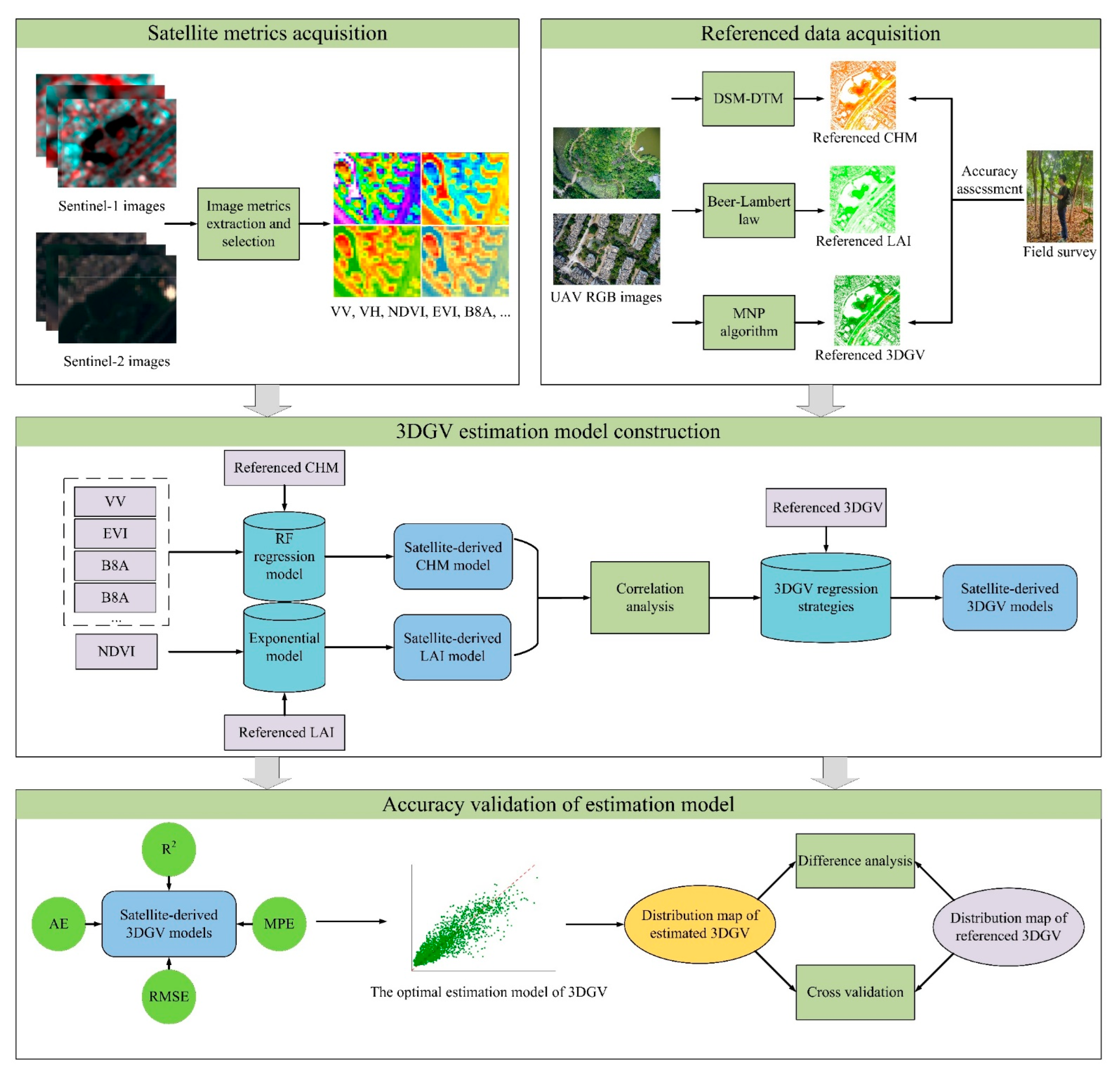
2. Materials and Methods

The detailed workflow of 3DGV retrieval in our research is displayed in Figure 1. Firstly, we acquired UAV RGB images and measured vegetation parameters including crown height and diameter. Using the UAV RGB images, we extracted CHM and calculated LAI based on Digital Surface Model (DSM) and Digital Terrain Model (DTM) and the Beer–Lambert law, respectively. 3DGV was estimated by MNP algorithm, the CHM and 3DGV derived from UAV images were assessed by field measurements, and provided the referenced data to our study. Secondly, two backscatter coefficients with polarization modes of Vertical–Vertical (VV) and Vertical–Horizontal (VH), spectral bands, and image metrics were extracted from Sentinel-1 and Sentinel-2 level 1C (L1C). The metrics selected by feature selection were combined with UAV-derived LAI and CHM to estimate satellite-derived LAI and CHM based on exponential model and RF regression model, respectively. Then, the satellite-derived LAI and CHM were employed to combine the UAV-derived 3DGV to construct estimation models of 3DGV based on their correlation relationships. Finally, accuracy of various models was assessed and compared to select the 3DGV estimation model with the highest accuracy, and further evaluated performance of the optimal estimation model by difference analysis and cross-validation using the distribution map of referenced 3DGV.

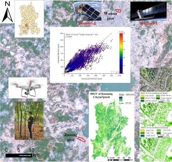
2.1. A Brief Description of Study Area and Study Sites

Kunming is one of China’s major garden cities; it is known as one of the most livable cities with high green coverage in China. It is located in the subtropical highland monsoon climate zone with low latitudes, which enjoys abundant sunshine, short frost periods, sufficient rainfall, and experiences minimal temperature fluctuations throughout the year. The study sites focus on two specific regions within Kunming City, both exhibiting favorable conditions for plant growth due to ample sunshine and sufficient rainfall, chosen to represent the vegetation distributions in UGS. The first region has a coverage area of 1.12 km², and is located around YueYaTan Park in Wuhua District (25°05′20″N~25°06′00″N, 102°43′00″E~102°44′0″E). The second region covers an area of 1.45 km², and surrounds ZhengHe Park in Jinning District (24°39′40″N~24°41′00″N, 102°35′00″E~102°36′30″E) (Figure 2). These regions offer different distributions of vegetation species and density, allowing for the comprehensive analysis of 3DGV in different urban landscapes.

2.2. Data Acquisition and Processing

2.2.1. Sentinel-1 Images

The Sentinel-1 satellite carries C-band Synthetic Aperture Radar (SAR), which is widely used for earth observation and forest source inventory [25]. For SAR Sentinel-1, we collected 1-level ground range detected products (GRD) from Google Earth Engine (GEE) in the interferometric wide (IW) swath mode in descending pass direction. Two backscattering coefficients under two polarization modes of VV and VH from 15 April 2022 to 15 May 2022 were extracted. The backscatter, integral to the radar signal, measures the extent to which a target redirects the radar signal back to the antenna. This measurement reflects the target’s reflective strength. We calculated the median image in this period, and resampled it to 10 m spatial resolution.

2.2.2. Sentinel-2 Images

The combination of Sentinel-1 and Sentinel-2 enables the generation of estimation products of vegetation structure attributes [24,31]. Sentinel-2 satellite carries a bivariate spectral imager (MSI), and it covers 13 spectral bands with spatial resolutions of 10 m, 20 m, and 60 m. The field of view spans 290 mm, with a revisit interval of five days, all conducted under a consistent viewing angle. For Sentinel-2, we collected Sentinel-2 L1C images from 15 April 2022 to 15 May 2022 in the GEE platform. Images were processed for atmospheric correction, cloud masking, and median composition, and then they were resampled to 10 m spatial resolution.

For accurately calculating parameters of vegetation, the extraction of pure vegetated pixels was important. NDVI threshold method was considered to achieve this, which was widely used to extract vegetation area and has been proven to be an effective and rapid method without depending on other a priori information [32,33]. Additionally, the Otsu algorithm, a reliable method for determining the NDVI threshold to extract vegetation [34,35], was used to capture the NDVI threshold in our study. The Otsu algorithm represents an automated and streamlined approach for achieving image segmentation based on clustering. This method efficiently determines the optimal threshold by associating each pixel’s grey value and subsequently evaluating inter-class variance.

In processed Sentinel-2 images of our research, we calculated NDVI in two plots and captured the NDVI threshold using the Otsu algorithm, which was 0.28. We randomly created 2000 sample pixels in two types and validated vegetation extraction accuracy, which showed that the overall accuracy was 91.72% and Kappa coefficient was 0.91. The vegetated areas extracted by NDVI threshold are displayed in Figure 3. All the data used in the study were masked by these vegetated areas, ensuring that only the pure vegetation pixels were included in the analysis.

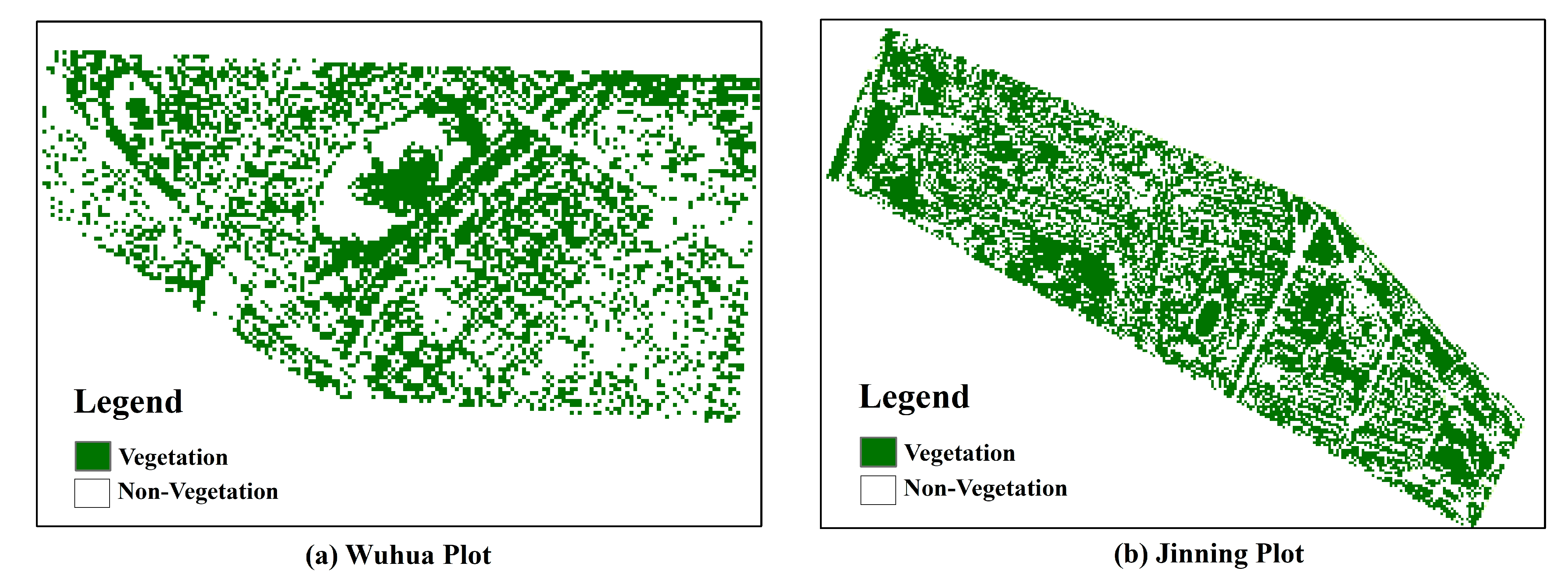
2.2.3. Acquisition and Preprocessing of UAV Images

The four-rotor DJI Phantom 4 RTK (SZ DJI Technology Co., Shenzhen, China) was employed to collect UAV RGB images on 29 April 2022, with a resolution of 7952 × 5304 pixels in JPG format. GPS location was obtained by using WGS-84 coordinate system. The flight route was defined at the ground station, and the UAV flown at 60 m to provide an image spatial resolution of 0.02 m. In terms of flight direction, the primary orientation encompassed an east-to-west trajectory, while the secondary orientation involved a north-to-south movement. These directions were characterized by forward and side overlaps of 80% and 70%, respectively. UAV was flown in excellent weather conditions, and sustained approximately 30 min to around study sites.

After ortho mosaicking, the aerial photographs yield ortho RGB images in the study sites. Then, the visible light vegetation indices, such as Visible Band Difference Vegetation Index (VDVI), and texture features were used to extract high-resolution vegetation regions. Visible light vegetation indices and texture features were widely used to map land cover based on RGB images, especially extracted vegetation regions [36,37]. We referred to previous studies and applied the Random Forest model [21,36] to classify vegetation and non-vegetation, achieving an accuracy of 93.86% and Kappa coefficient of 0.93.

Subsequently, we defined the fishnet on study sites with a size of 1 m to calculate all UAV-derived parameters. The fishnet was used to calculate the parameters derived from UAV, including vegetation coverage, CHM, and 3DGV. Pix4D desktop was employed to produce point data and generate DSM and DTM. A total of 25 ground control points (GCPs) were set to correct the accuracy of DSM. The median of point in two plots was 12,312.6 and 11,940.9 for matching each image, and the surface density was 56.14/m² and 61.87/m², respectively. CHM was calculated by difference of DSM and DTM, and the vegetation coverage was computed by percentage of vegetation pixels in each cell. Then, 3DGV was estimate based on the MNP algorithm [21], and the formulas were as follows:

$$CH{M}_{\mathrm{i}}=DS{M}_i-DT{M}_{\mathrm{i}}$$

(1)

$$C_{\mathrm{i}}=\frac{N_v}{N_T}$$

(2)

$$G={\displaystyle \sum _i^j{S}_i\times CHM}\times C_{\mathrm{i}}$$

(3)

where G is 3DGV, $i$ is cell number, $j$ is the total cell number, $S_i$ is pixel area of cell, $CH{M}_{\mathrm{i}}$ is the canopy height of cell, $C_{\mathrm{i}}$ is vegetation coverage of cell, $DS{M}_i$ is the average DSM of cell, and $DT{M}_i$ is the average DTM of cell. $N_v$ is vegetated pixels number of cells, and $N_T$ is total pixel number of cells.

The LAI derived from UAV data was calculated based on the Beer–Lambert law, which describes the relationship between LAI and light transmittance through the canopy vegetation. Previous researchers have described this relationship by relating LAI to vegetation coverage [16,19,38]. The calculation formulas were as follows:

$$\Omega (\theta )=\frac{In(\overline{1-C_{\mathrm{i}}})}{\overline{In(1-C_{\mathrm{i}})}}$$

(4)

$$\mathrm{LAI}=-\frac{\cos \theta \times In(1-C_{\mathrm{i}})}{G(\theta )\times \Omega (\theta )}$$

(5)

where the θ is the observation zenith angle, and it is considered to be 0 degrees due to the ortho photo, G(θ) represents the average projected area of foliage per unit area in the plane perpendicular to the measurement direction, and is related to the distribution of leaf angles and is typically assigned a value of 0.5 [38], and Ω(θ) represents the clumping index, which depends on the spatial distribution of leaves.

All UAV-derived parameters were estimated as the reference data in 1 m cells. In order to combine with satellite images, we defined a new fishnet with a size of 10 m on orthophotos to register and correct with satellite images at 10 m spatial resolution. The 10 m vegetation coverage and CHM were calculated by the mean vegetation coverage and CHM of all included 1 m cells, respectively, and the 10 m 3DGV was calculated by the sum 3DGV of all included 1 m cells.

2.2.4. Field Measurements

Field measurement was performed on 3 May 2022. We employed a real-time kinematic instrument, the ZHDV200 (RTK, GNSS, Guangzhou Hi-Target Navigation Tech Co., Ltd., Guangzhou, China), to accurately establish the boundaries and coordinates of sample plots. These plots, measuring 10 m × 10 m, were strategically distributed across the study sites, totaling 60 in number. Tree parameters were measured by handheld digitalized bivariate functional forest measurement gun and tape measure [39], including tree height, crown diameter, and first branch height. In addition, according to the main tree species in study sites, we used the empirical formulas in previous studies to calculate 3DGV, which can result in an average relative bias of 16.4% and an average relative RMSE of 12.5% [11]. The empirical formulas of 3DGV in previous studies are listed in

Table 1. 3DGV empirical formulas of various vegetation species.

Tree Species	Geometrical Morphology	Calculation Formula	Description
Metasequoia glyptostroboides Hu and W.	cone	$\pi \cdot a^2\cdot b/12$	$a$represents crown diameter and $b$ represents crown height.
Salix babylonica L.	ovoid	$\pi \cdot a^2\cdot b/6$
Elaeis guineensis Jacq.
Osmanthus fragrans Makino.	sphere	$\pi \cdot a^2\cdot b/6$
Cinnamomum japonicum Sieb.
Ficus microcarpa L.f.
Elaeocarpus decipiens Linn.	flabellate	$\pi \cdot (2a^3-a^2\cdot 4a^2-b^2)/3$
Cycas revoluta Thunb.

.

The referenced parameters derived from UAV were assessed by field measurements, the mean CHM of plots achieved a bias of 1.34 m (18.34%) and a RMSE of 1.79 m (21.64%), and the mean 3DGV of plots resulted in a relative bias of 107.34 m³ (16.29%) and a relative RMSE of 142.47 m³ (20.09%).

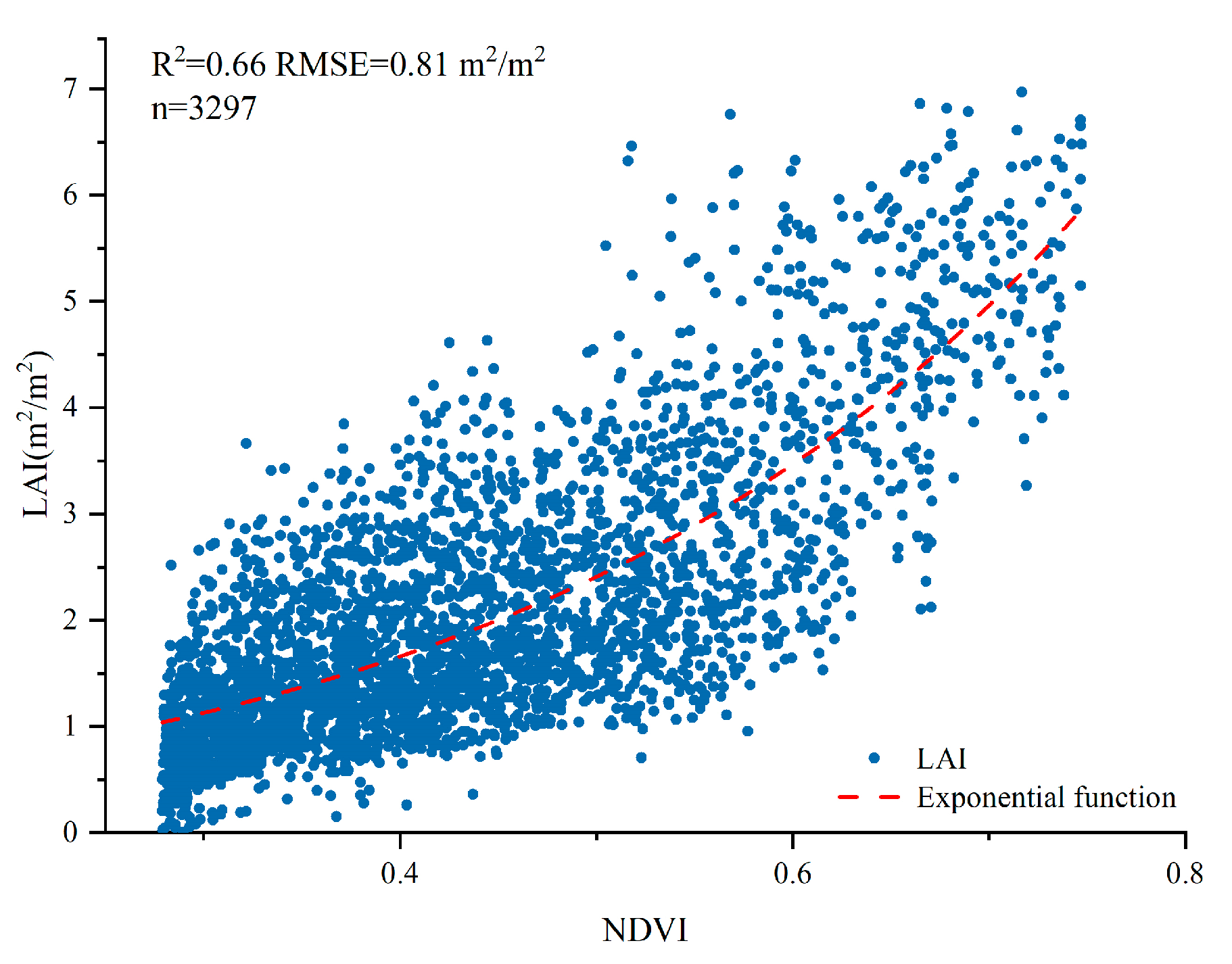
2.3. Calculating LAI Derived from Satellite Images

Previous studies have shown that the non-linear models have better performance than linear models in the estimation of LAI based on Sentinel-2 images [40]. In addition, among the common non-linear models, the exponential model established by NDVI can result in excellent accuracy in LAI estimation [41,42]. We selected this method to estimate satellite-derived LAI based on Sentinel-2 images. The formula of the function was as follows:

$$LAI=a\cdot e^{b\cdot NDVI}+c$$

(6)

Figure 4 displays the correlation relationship between UAV-derived LAI and NDVI derived from Sentinel-2. They fitted an exponential regression and were validated in validation set with R² of 0.66, and the regression model was described as in Equation (7).

$$LAI=0.44\cdot e^{3.57\cdot NDVI}-0.12$$

(7)

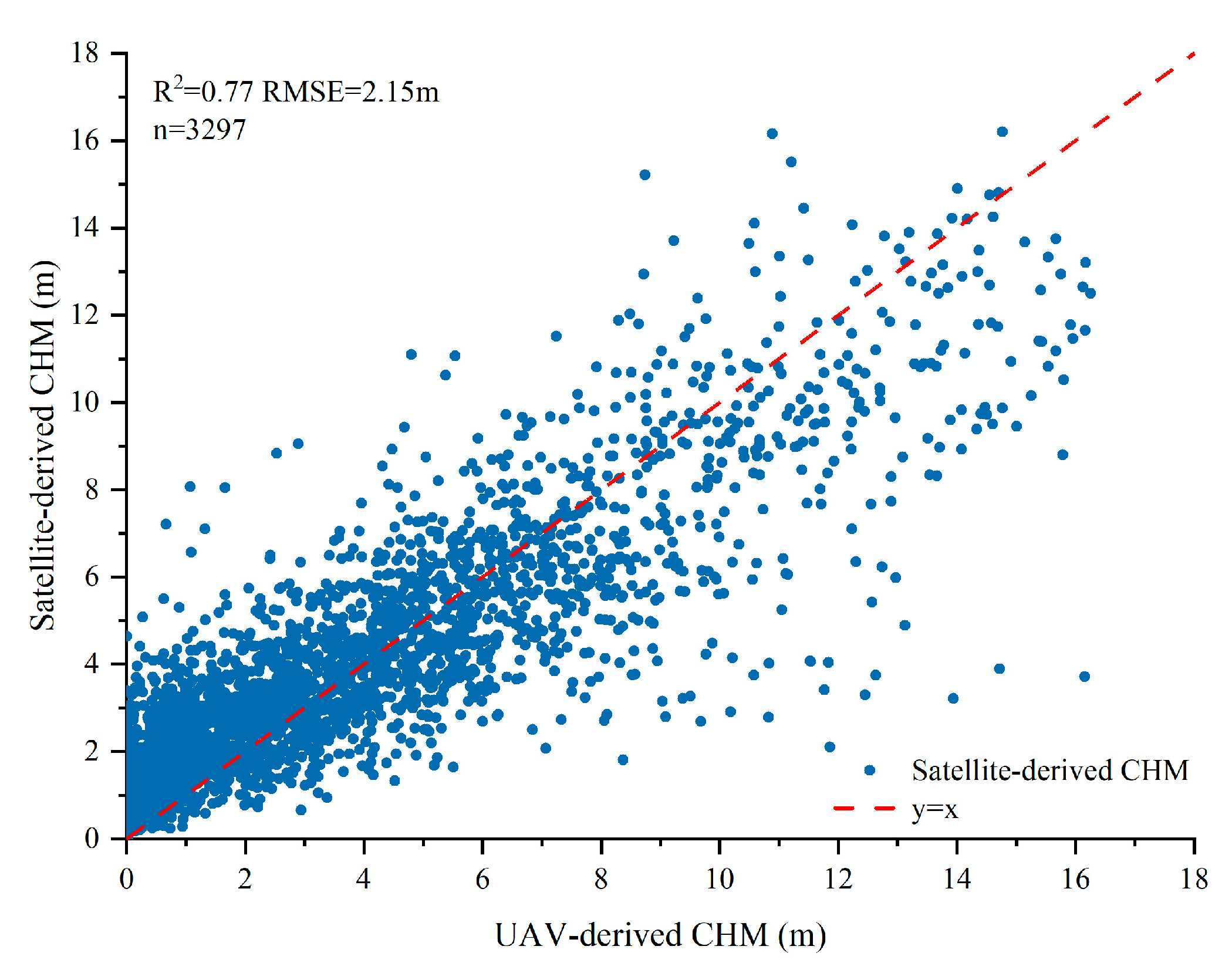
2.4. Calculating CHM Derived from Satellite Images

In CHM extraction from satellite images, the Random Forest (RF) regression model was widely used in previous studies [24,31,43]. RF is a machine learning method that constructs independent decision trees iteratively during training [44]. RF can effectively handle a substantial number of predictor variables without falling into the trap of overfitting, and is less susceptible to noise in the training data [45]. We used RF regression model with a decision tree number of 200 to estimate the satellite-derived CHM. A total of 11 spectral bands and 11 vegetation indices were obtained from Sentinel-2, along with two backscatter coefficients from Sentinel-1; their difference and quotient were selected as relevant variables. All variables were evaluated for their importance using RF feature importance assessment, and the correlation between the related variables was calculated by Pearson correlation analysis. This importance score represents the ratio of the average error to the standard deviation derived from the variable predictions across each decision tree in RF algorithm, and Pearson correlation analysis was used to eliminate potential multicollinearity issues between variables. The feature selection is exhibited in Figure 5. When the importance score was higher than 0.5 and the correlation coefficient exceeded 0.7, the feature was retained in this model. The total of 10 selected features are listed in

Table 2. The variables used in satellite-derived CHM modeling.

Variable	Formula	Explanation	Attribute
VH	$\sigma =sigma\times \cos \alpha$	Backscatter coefficient of VV (Vertical–Vertical) polarization modes	σ represents the backscatter coefficient after the projection angle correction, sigma represents the radar brightness value. α represents the projection angle.
VV		Backscatter coefficient of VH (Vertical–Horizontal) polarization modes
VV/VH
LSWI	$(B8-B11)/(B8+B11)$	Land surface water index	B8 is NIR (Wavelength = 842 nm), B4 is red band (Wavelength = 665 nm), B3 is green band (Wavelength = 560 nm)
EVI	$2.5\times (B8-B4)/(B8+6\times B4-7.5\times B2+1)$	Enhanced vegetation index
B2			NIR (Wavelength = 705 nm)
B6			NIR (Wavelength = 705 nm)
B8			NIR (Wavelength = 842 nm)
B8A			NIR (Wavelength = 865 nm)
B11			SWIR (Wavelength = 1610 nm)

.

The comparison between satellite-derived CHM and UAV-derived CHM in validation set is shown in Figure 6, which achieved R² was 0.77. The distribution map of UAV-derived 3DGV, satellite-derived LAI and satellite-derived CHM at 10 m resolution in two study sites is displayed in Figure 7.

2.5. Construction of 3DGV Estimation Models

On the basis of satellite-derived LAI and CHM, univariate and bivariate parametric models were employed to explore the optimal retrieval model. Five strategies were used for univariate estimation models based on LAI or CHM, including linear model, exponential model, power model, logarithmic model, and polynomial model [46]. The variable combination of LAI and CHM was used to construct bivariate models of linear model, exponential model, power model, logarithmic model, and polynomial model [47]. Furthermore, we compared two kinds of univariate models to select two optimal models based on LAI and CHM, respectively. According to the stand-level volume models, we combined the two optimal univariate models of LAI and CHM through multiplication [48], and constructed a compound model to regress 3DGV.

2.6. Accuracy Assessment of Estimation Models

A total of 10,989 samples were randomly partitioned into 7692 training samples and 3297 validation samples at a ratio of 7:3. The constructed estimation models were evaluated using the validation data sets. Pearson correlation coefficient (R) was used to analyze the correlation relationship between 3DGV training set and predictor variables, and four accuracy assessment metrics—root mean square error (RMSE), coefficient of determination (R²), mean absolute error (MAE), and mean prediction error (MPE)—were employed to assess the accuracy of estimation models using the 3DGV validation set. Furthermore, the significance of models was tested at the significance level of 0.05. The formulas for metrics that we used are defined as follows:

$$R=\frac{Cov(y_r,y_i)}{\sqrt{\mathrm{var}\left|y_r\right|\times \mathrm{var}\left|y_i\right|}}$$

(8)

$$R^2=1-\frac{{{\displaystyle {\sum }_{i=1}^n(y_r-y_i)}}^2}{{{\displaystyle {\sum }_{i=1}^n(y_r-\overline{y_r})}}^2}$$

(9)

$$RMSE=\sqrt{\frac{{{\displaystyle {\sum }_{i=1}^n(y_r-y_i)}}^2}{n-1}}$$

(10)

$$MAE={\displaystyle {\sum }_{i=1}^n\frac{\left|y_r-y_i\right|}{n}}$$

(11)

$$MPE=t\times \frac{\sqrt{\frac{{{\displaystyle {\sum }_{i=1}^n(y_r-y_i)}}^2}{n-q}}}{\overline{y_r}}/\sqrt{n}\times 100$$

(12)

where $y_i$is retrieved value of models, $y_r$ is the reference value of UAV data, $\overline{y_r}$ is the average value of $y_r$, $Cov$ is covariance, $Var$ is variance, $n$ is the total number of reference data, $q$ is the number of parameters in modeling, and $t$ is the t-value at confidence level of 0.05.

For the selected model comparing all 3DGV estimation models, we employed cross-validation to validate its accuracy in several ranks and generated the confusion matrix [49]. The accuracy of this model was evaluated by using producer’s accuracy (PA), user’s accuracy (UA), and overall accuracy (OA). Furthermore, fraction vegetation coverage (FVC) was also introduced to compare with 3DGV, and it was inverted by NDVI based on the pixel dichotomous model. After validating the accuracy, we extended the model to cover the entire city of Kunming, and compared it with CHM, LAI, and FVC to analyze the effectiveness of our model. We selected the maximum and minimum values of the NDVI in the study area instead of the ${NDVI}_{veg}$ and ${NDVI}_{soil}$ values [50]. That is, the NDVI values corresponding to a cumulative frequency of 2% were taken as NDVI soil, and the NDVI values corresponding to a cumulative frequency of 98% were taken as ${NDVI}_{veg}.$ The formula was as follows:

$$FV{C}_{\mathrm{i}}=(NDV{I}_{\mathrm{i}}-NDV{I}_{soil})/(NDV{I}_{vegtation}-NDV{I}_{soil})$$

(13)

where ${NDVI}_{veg}$ is the NDVI value of the pure vegetation pixel and ${NDVI}_{soil}$ is the NDVI value of the pure non-vegetation pixel.

3. Results

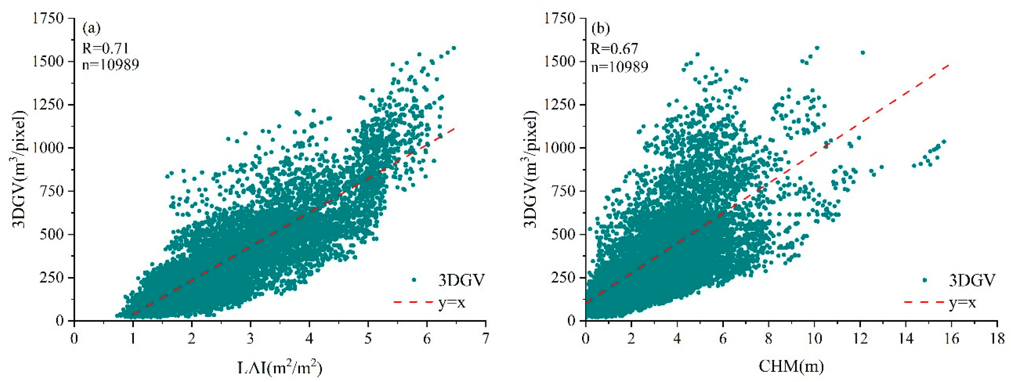
3.1. Univariate Estimation Models of 3DGV

All samples (n = 10,989) were used to analyze the correlation relationships between LAI and 3DGV, and CHM and 3DGV; the correlation relationship of LAI and 3DGV (R = 0.71) was stronger than CHM and 3DGV (R = 0.67) (Figure 8). Five 3DGV estimation models (Figure 9) based on LAI and CHM were fitted using the training sets (n = 7692), and we compared their accuracy using the validation sets (n = 3297). The average RMSE of LAI models was 183.72 m³/pixel and CHM models were 235.91 m³/pixel, indicating that LAI performed better than CHM for 3DGV retrieval (

Table 3. Accuracy assessment of 3DGV estimation using validation set based on univariate models.

	Regression Model	Formula	R2	RMSE (m3/Pixel)	AE (m3/Pixel)	MPE (%)	p-Value
3DGV models based on LAI	Linear model	$3DGV=201.4\cdot LAI-197.51$	0.61	168.89	151.73	12.45	<0.05
	Exponential model	$3DGV=617.36\cdot e^{0.18\cdot LAI}-606.59$	0.67	146.17	129.94	11.43	<0.05
	Power model	$3DGV=71.4\cdot LA{I}^{1.55}-16.09$	0.68	144.92	126.81	11.07	<0.05
	Logarithmic model	$3DGV=309.19\cdot \ln (LAI+0.75)$	0.36	313.26	276.14	24.08	>0.05
	Polynomial model	$3DGV=89.19\cdot LAI+18.52\cdot LA{I}^2-57.04$	0.67	145.34	128.75	11.21	<0.05
3DGV models based on CHM	Linear model	$3DGV=68.99\cdot CHM+92.18$	0.59	180.68	163.25	13.37	<0.05
	Exponential model	$3DGV=-1280.17\cdot e^{0.12\cdot CHM}+1408.25$	0.43	256.45	234.71	19.71	>0.05
	Power model	$3DGV=65.3\cdot CH{M}^{1.22}-24.72$	0.49	234.46	217.04	17.82	>0.05
	Logarithmic model	$3DGV=340.64\cdot \ln (CHM+0.69)+102.11$	0.4	273.75	258.31	20.65	>0.05
	Polynomial model	$3DGV=-4.15\cdot CH{M}^2+142.86\cdot CHM+34.45$	0.51	234.19	206.58	17.16	<0.05

). Among all univariate models, the power model based on LAI (R² = 0.68, RMSE = 144.92 m³/pixel, AE = 126.81 m³/pixel, MPE = 11.07%, p < 0.05) and the linear model based on CHM (R² = 0.59, RMSE = 180.68 m³/pixel, AE = 163.25 m³/pixel, MPE = 13.37%, p < 0.05) achieved the highest accuracy. The density scatter graphs (Figure 10) between the estimated 3DGV of two optimal models and reference 3DGV were plotted to analyze the variation of all samples. We found that the scatters of optimal models were concentrated around the reference line, and the variation was mainly distributed in low density areas. The overestimation occurs in the areas with low 3DGV values while the underestimation occurs at the areas with high 3DGV values, and the performance of 3DGV power model based on LAI (Figure 10a) was better than the 3DGV linear model based on CHM (Figure 10b).

3.2. Bivariate Estimation Models of 3DGV

The optimal bivariate estimation model of 3DGV was selected based on accuracy assessments (

Table 4. Accuracy assessment of 3DGV estimation using validation set based on bivariate models.

	Regression Model	Formula	R2	RMSE (m3/Pixel)	AE (m3/Pixel)	MPE (%)	p-Value
Bivariate models	Linear model	$3DGV=170.09\cdot LAI+24.42\cdot CHM-173.01$	0.68	142.78	127.59	10.96	<0.05
	Exponential model	$3DGV=651.03\cdot e^{0.15\cdot LAI+0.02\cdot CHM}-697.56$	0.76	126.17	109.94	8.94	<0.05
	Power model	$3DGV=69.42\cdot LA{I}^{1.29}CH{M}^{0.24}-19.72$	0.77	124.92	106.81	8.83	<0.05
	Logarithmic model	$\begin{array}{l}3DGV=482.65\cdot \ln (1.12\cdot LAI)\\ +45.15\cdot \ln (0.87\cdot CHM)-97.54\end{array}$	0.53	227.94	199.83	16.45	<0.05
	Polynomial model	$\begin{array}{l}3DGV=49.43\cdot LAI-11.2\cdot LAI\cdot CHM+49.47\cdot CHM\\ +1.12\cdot LA{I}^2\cdot CHM+20.25\cdot LA{I}^2-37.04\end{array}$	0.77	130.94	106.71	9.19	<0.05
	Compound model	$3DGV=37.13\cdot LA{I}^{-0.3}\cdot CHM+38.62\cdot LA{I}^{1.8}+13.8$	0.78	122.36	103.98	8.71	<0.05

). The compound model achieved the highest accuracy (R² = 0.78, RMSE = 123.36 m³/pixel, AE = 103.98 m³/pixel, MPE = 8.71%, p < 0.05). Note that the average RMSE was 175.02 m³/pixel. Compared to the optimal univariate models, the compound model performed better than all univariate models (Table 3). Except for the bivariate logarithmic model, the accuracy of the bivariate models was consistently higher than all univariate models, which implies that the combination of LAI and CHM can effectively improve the accuracy of 3DGV estimation. In addition, the density scatter graphs between the estimated 3DGV of the compound model and the referenced 3DGV also demonstrated its superiority (Figure 11). Scatters concentrate around the reference line from low 3DGV to high 3DGV, and a slight overestimation occurs in the areas with low 3DGV values while the underestimation occurs in the areas with high 3DGV values (Figure 11). Thus, we selected the compound model to map the 3DGV to observe the spatial distribution details and further verified the mapping accuracy in Section 3.3.

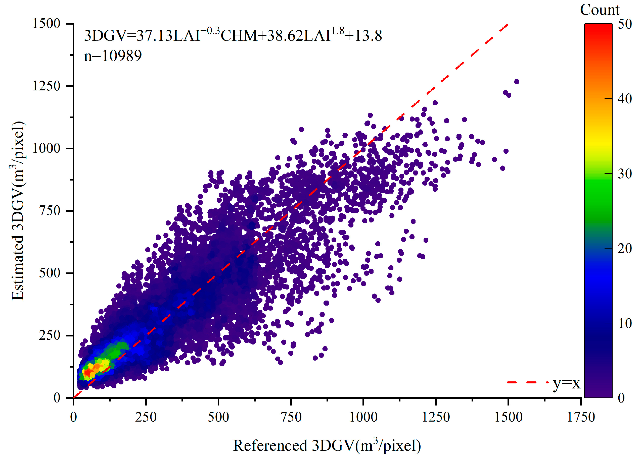
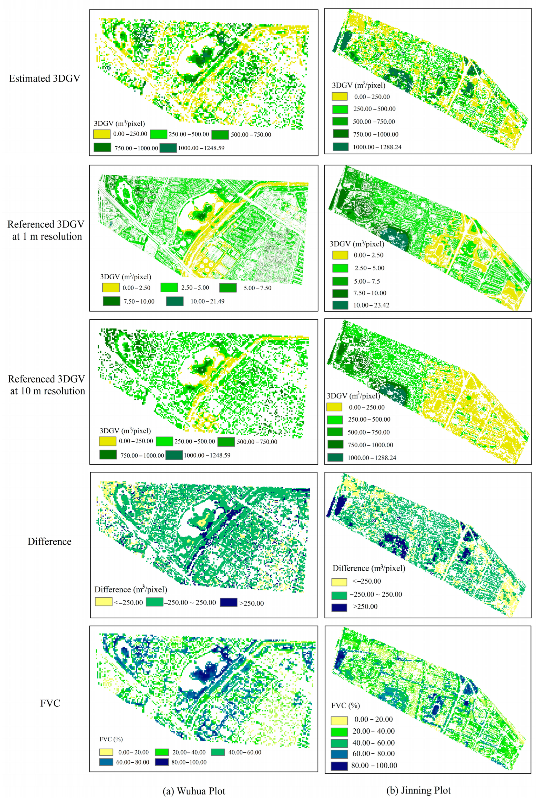
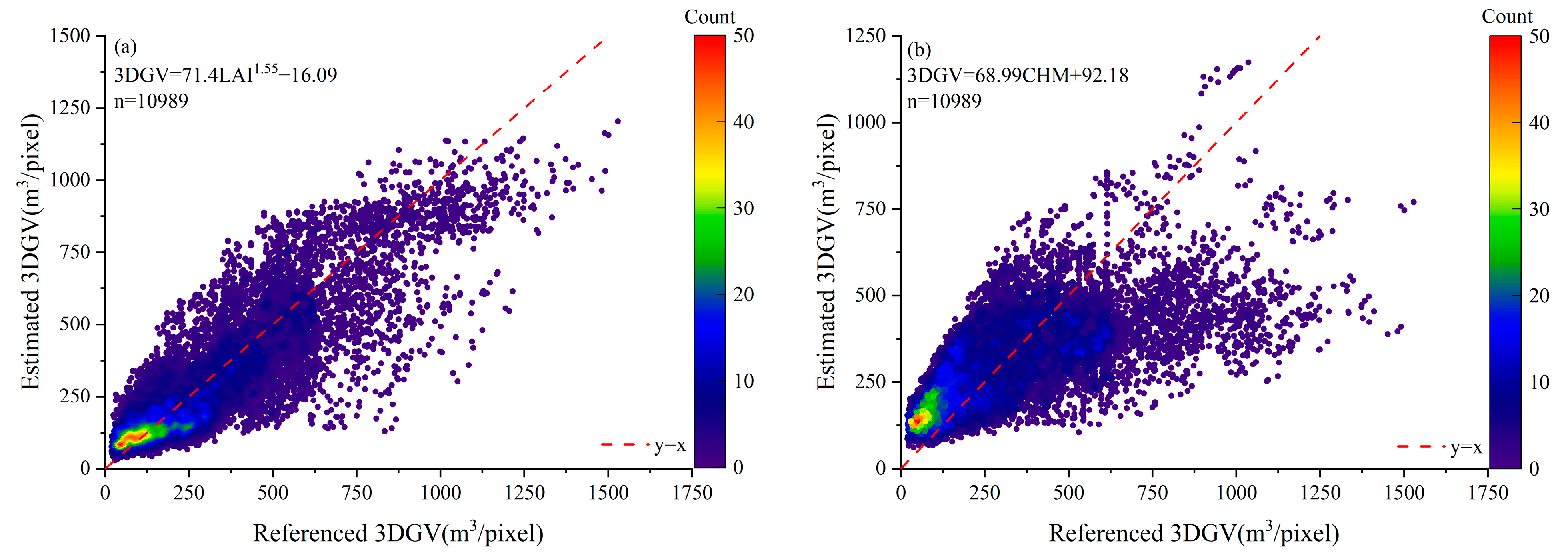
3.3. Validation of Estimated 3DGV

The compound model regressed in Section 3.2 was introduced to estimate 3DGV for entire study sites. The total estimated 3DGV for the Wuhua plot and Jinning plot were 3,697,133.85 m³ and 2,654,830.43 m³, respectively. To evaluate the mapping accuracy of the estimated 3DGV, we divided the estimated 3DGV into four interval ranks for cross-validation; the performance is summarized in the confusion matrix and presented in

Table 5. The confusion matrix of estimated 3DGV.

3DGV	0–250 m3/Pixel	250–500 m3/Pixel	500–750 m3/Pixel	>750 m3/Pixel	Total
0–250 m3/pixel	3936	852	163	0	4951
250–500 m3/pixel	972	2992	110	65	4139
500–750 m3/pixel	132	124	944	123	1323
>750 m3/pixel	17	85	89	385	576
Total	5057	4053	1306	573	10,989
PA/%	79.50	72.29	71.35	67.07
UA/%	77.83	73.82	72.39	67.19
OA/%	75.15

. Furthermore, we calculated the sum of reference 3DGV at 10 m resolution, and Figure 12 provides the visual representations of distribution of estimated 3DGV, reference 3DGV, and FVC in the study sites. For comparison, we also mapped the difference between estimated and referenced 3DGV at 10 m resolution.

In Figure 12, the difference distribution map revealed only a few regions where the estimated values deviate either positively or negatively from the reference values. In addition, FVC distribution maps displayed the 3DGV overestimation tends to occur in are-as with lower FVC value, while underestimation tends to occur in areas with higher FVC value. Table 5 presents the cross-validation of the 3DGV estimation model. The model exhibited its best performance in the rank of 0–250 m³/pixel (PA = 79.50%, UA = 77.83%), and the accuracy in the rank of 250–500 m³/pixel (PA = 72.29%, UA = 73.82%) and 500–750 m³/pixel (PA = 71.35%, UA = 72.39%) was relatively similar. Note that the model performed worst in the rank of >750 m³/pixel (PA = 67.07%, UA = 67.19%), and we have identified two potential reasons for the lower accuracy obtained in our results. One reason was the constraints of the estimation model which tended to underestimate the values compared to the reference data; this underestimation can be observed in scatter plots (Figure 11). This bias in estimation may decrease the estimated value in higher 3DGV ranks, and contribute to the lower accuracy. Another reason was the lack of 3DGV samples exceeding 750 m³ in our study sites. The model might not have sufficient training data to accurately estimate 3DGV in higher 3DGV ranks. In summary, although the model can cause minor deviations of estimation, the compound model can effectively capture the distribution pattern to 3DGV in UGS, and it still achieves superior accuracy in 3DGV estimation.

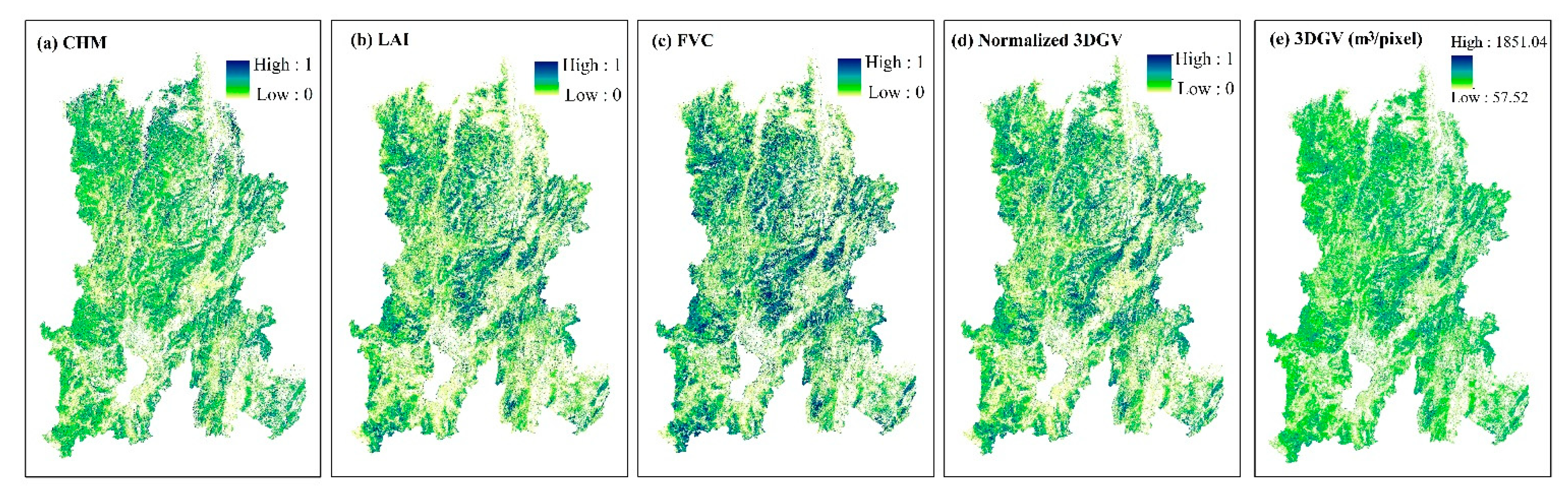
3.4. Spatial Pattern of 3DGV in Kunming City

To verify the applicability of the optimal model at a large scale, this model was used to map 3DGV in Kunming city. Due to the lack of UAV-derived referenced data in whole of Kunming city, we only used the spatial distribution maps of CHM, LAI, and FVC to verify the consistent of 3DGV spatial distribution in Figure 13a–d, and all the values were normalized in advance at 10 m spatial resolution. In addition, we also mapped the retrieved 3DGV in Kunming in Figure 13e. The maximum value of 3DGV is 1851.04 m³/pixel, the minimum value is 57.52 m³/pixel, and the average value is 553.77 m³/pixel. From the spatial distribution pattern of 3DGV, it can be seen that 3DGV was higher in the central and northwest areas, and lower in northeast and southeast areas. When compared to the other characteristics, 3DGV was well consistent with CHM, LAI, and FVC in spatial distribution pattern.

4. Discussion

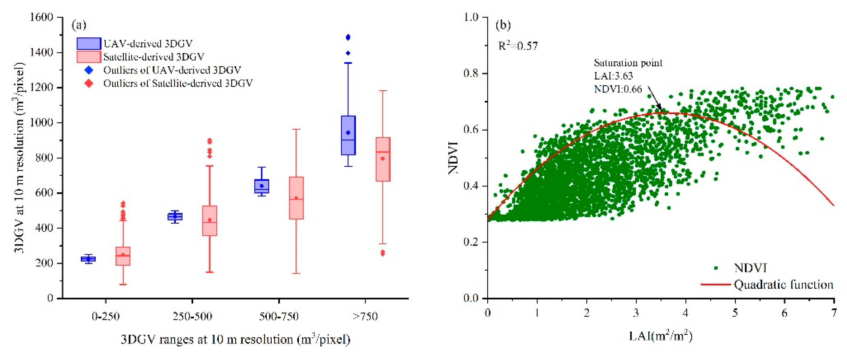
4.1. Analyzing the Effect of NDVI Saturation and Spatial Resolution of Sentinel Images

3DGV retrieval by satellite-derived LAI and CHM can achieve good accuracy, but some inevitable effects were caused by various sources. To analyze these effects, we calculated the sum of UAV-derived 3DGV at 10 m resolution, and randomly selected a total of 1000 samples within four ranks based on the sum of UAV-derived 3DGV. Figure 14a illustrates the UAV-derived and satellite-derived 3DGV of samples, respectively. It can be observed that in the rank of 0–250 m³/pixel, our model tends to overestimate, but the model tends to underestimate with the increase of 3DGV values, especially in the rank of >750 m³/pixel. This change was also analyzed from our results. We considered that this might be due to the saturation of NDVI, so we used UAV-derived LAI as an independent variable and NDVI as the dependent variable to explore this saturation issue based on a quadratic function. The independent variable corresponding to the extreme value of the function in the interval is the LAI saturation point [50]. As shown in Figure 14, LAI and 3DGV fit a functional relationship with a R² of 0.57, and the NDVI was 0.66, reaching saturation point when LAI was 3.63. Although some scholars have shown the correlation relationship of them [41,42], it would also influence the 3DGV value to be underestimated in high 3DGV, especially in areas with dense vegetation.

In addition, 3DGV estimation in our research was conducted at a 10 m spatial resolution based on satellite images, but the reference 3DGV was computed at a higher spatial resolution of 1 m. We founded that the estimation realized based on satellite images would cause underestimation. To analyze these effects, the image details of different spatial resolutions were displayed in Figure 15, in order to describe the limitations of satellite-derived 3DGV compared to UAV-derived 3DGV. From the comparisons, the UAV-derived 3DGV accurately displayed the detailed vegetation information in the selected regions (Figure 15b), but the satellite-derived 3DGV exhibited some limitations in capturing detailed vegetation information (Figure 15a). The pixel coverage of satellite-derived 3DGV is insufficient in sparse areas, such as the roadside trees or individual potted plants. Although the inaccurate vegetation extraction might contribute to this effect, we believed that this insufficiency is due to the satellite images being unable to capture the smaller-scale vegetation elements. These limitations highlighted the challenges in estimating regional 3DGV, and except for the model’s estimation bias, there was an additional concern of vegetation information gaps.

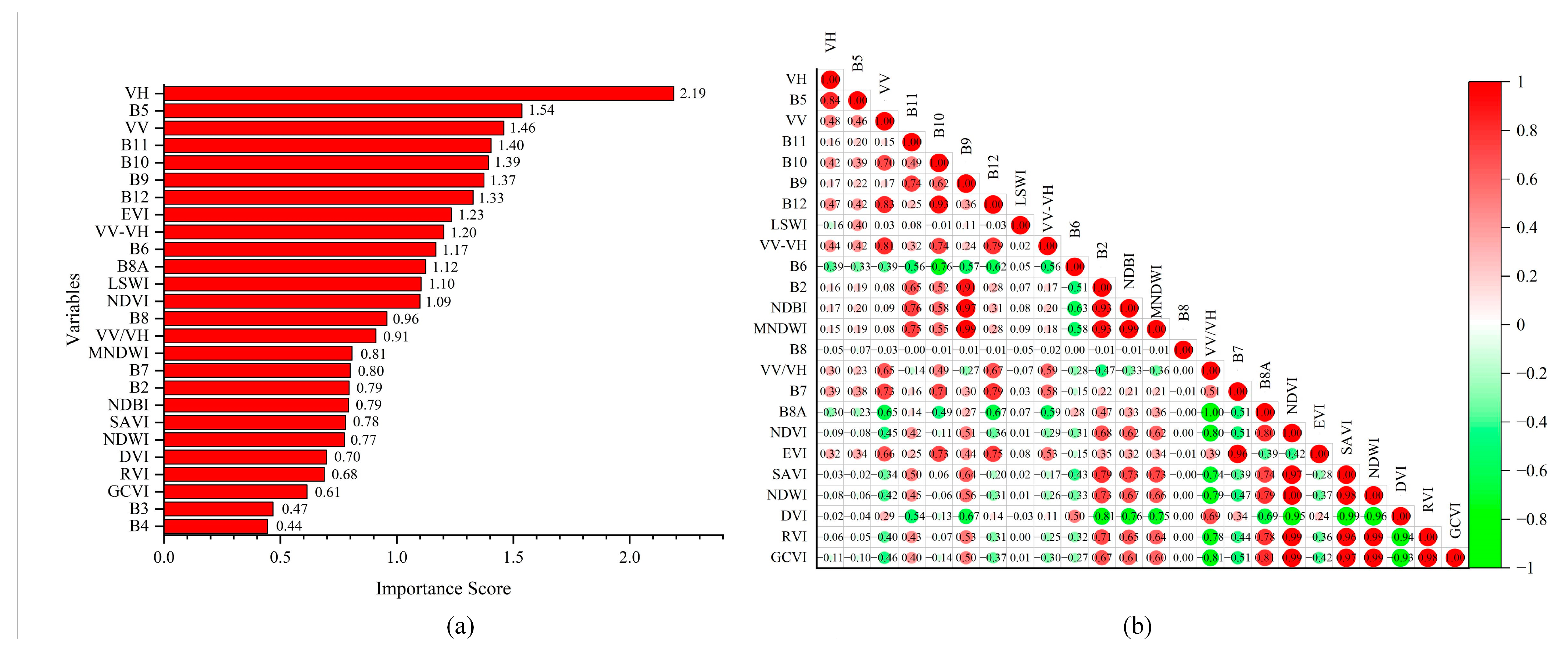
4.2. Predictor Variables Selection

In terms of predictor variables, 3DGV is a parameter which reflects vegetation spatial structure, and the estimation of vegetation structure characteristics is typically based on various biophysical parameters, such as vegetation cover and biomass [31,51,52]. We used two variables that also reflect vegetation structure for estimation, which are relatively easier to obtain compared to the vegetation cover and biomass [53,54]. LAI is a widely accepted indicator to evaluate the ecological quality of UGS, as it is closely related to plant growth, biomass, and photosynthetic activity [55]. On the other hand, CHM provides valuable information about vegetation structure and directly reflects the vertical structure of ecosystems [56]. Another reason is that previous studies have estimated similar indicators to 3DGV, such as timber volume and forest volume, which are calculated by combining area-based indicators with tree height measurements, such as basal area [48,57,58]. Taking inspiration from these studies, we selected LAI to replace the basal area as the area-based indicator and combined it with CHM for the 3DGV estimation.

In future research, the 3DGV estimation model w extended to larger scales. We will consider incorporating other remote sensing metrics to construct the estimation model, such as spectral bands [25], vegetation indices, and texture features [59], in order to further improve the accuracy of 3DGV estimation. Furthermore, we will collect much measured data and enrich different vegetation samples to enhance the applicability of the estimation model for different seasons, different areas, and different development levels of UGS in cities.

4.3. Limitations and Strengths

Many researchers have been pursuing various methods for estimating 3DGV. In comparison to previous studies, our approach has made several advancements. For the estimation method, we did not use the MNP algorithm that was applied in UAV-derived 3DGV to apply in satellite-derived estimation. The MNP algorithm considers the pixels from high resolution images as voxels to estimate their volume [21], but the spatial resolution of satellite images is too low to further calculate the precise parameters in pixels. Our research used parametric models to retrieve 3DGV, which can result in similar accuracy compared to previous research studies with non-parametric models (relative error = 20.9% [60], estimation accuracy = 88.07% [17]). This level of consistency shows that the method of parametric models is feasible for 3DGV estimation. Furthermore, our method is also close to the accuracy of regional 3DGV estimation using LiDAR data (overall accuracy = 85% [61]), which can support their DGV estimation results based on SPOT5. Moreover, our results illustrate that the physical parameters of LAI and CHM, as well as spectral index and texture index, are superior for volume estimation (rRMSE = 61.42% [59]), and further demonstrated feasibility and potential for 3DGV estimation based on Sentinel-1 and Sentinel-2.

However, this study still has several limitations for improvement. Firstly, the predictor variables of satellite-derived LAI and CHM were both the estimated value, without field measurement. Although previous studies assessed the LAI accuracy of the exponential model constructed by NDVI [26], and the CHM accuracy of RF model established by Sentinel-1 and Sentinel-2 images [25], there may still be some biases from our reference data in which R² was 0.66 and 0.77, respectively. Secondly, the reference 3DGV was not the most accurate representation. The 3DGVs used in this research were calculated based on UAV RGB images, the accuracy of which were assessed in our previous study [21]. The MNP algorithm was overestimated compared to the measured data (Bias = 15.18%, RMSE = 19.63%, R² = 0.96). This overestimation was caused due to only the higher parts of the tree were calculated, resulting in the lower parts of the crown not being accurately considered. Lastly, our estimation model was constructed based on the overall vegetation distribution of UGS, but there was various vegetation. As a result, our model may not be applicable to all kinds of vegetation in UGS.

5. Conclusions

In summary, this study focused on 3DGV retrieval in UGS, and developed a parametric 3DGV estimation model by incorporating LAI and CHM derived from Sentinel-1 and Sentinel-2. Satellite-derived LAI and CHM revealed strong power and linear relationships to 3DGV derived from UAV images, respectively. The optimal univariate model of 3DGV was constructed based on LAI, which was regressed by power model and achieved an excellent accuracy (71.4·LAI^1.55 − 16.09, R² = 0.68, RMSE = 144.92 m³/pixel, AE = 126.81 m³/pixel, MPE = 11.07%, p < 0.05). The optimal bivariate model was a compound model that combines the power model of LAI and linear model of CHM, which can result in the highest accuracy (37.13·LAI^−0.3·CHM + 38.62·LAI^1.8 + 13.8, R² = 0.78, RMSE = 124.36 m³/pixel, AE = 103.98 m³/pixel, MPE = 8.71%, p < 0.05). The 3DGV of the optimal estimation model was found to achieve a good overall accuracy in study sites, and we concluded its spatial pattern was well consistent with CHM, LAI, and FVC within Kunming city. This result indicated that the ability of this 3DGV estimation model was suitable to apply in UGS, but it remains limited in that it performed better in vegetation with lower 3DGV and produced underestimation in vegetation with higher 3DGV. Our study developed a parametric 3DGV estimation model based on Sentinel-1 and Sentinel-2 images, which demonstrate the potential of extending 3DGV retrieval in UGS.

References

1. Nath, T.K.; Han, S.S.Z.; Lechner, A.M. Urban green space and well-being in Kuala Lumpur, Malaysia. Urban For. Urban Green. 2018, 36, 34–41. [Google Scholar] [CrossRef]
2. Dobbs, C.; Kendal, D.; Nitschke, C. The effects of land tenure and land use on the urban forest structure and composition of Melbourne. Urban For. Urban Green. 2013, 12, 417–425. [Google Scholar] [CrossRef]
3. Wolch, J.R.; Byrne, J.; Newell, J.P. Urban green space, public health, and environmental justice: The challenge of making cities ‘just green enough’. Landsc. Urban Plan. 2014, 125, 234–244. [Google Scholar] [CrossRef]
4. Wang, T.; Yang, X.; Hu, S.; Shi, H. Comparisons of methods measuring green quantity. China Acad. J. Electron. Publ. House 2010, 8, 36–38. [Google Scholar]
5. Chen, Z. Research on the ecological benefits of urban landscaping in Beijing (2). China Gard. 1998, 14, 51–54. [Google Scholar]
6. Zhou, J.H.; Sun, T.Z. Study on remote sensing model of three-dimensional green biomass and the estimation of environmental benefits of greenery. Remote Sens. Environ. China 1995, 3, 162–174. [Google Scholar]
7. Song, Z.; Guo, X.; Ma, W. Study on green quantity of green space along road in Beijing plain area. Jilin For. Sci. Technol. 2008, 37, 11–15. [Google Scholar]
8. Chen, F.; Zhou, Z.X.; Xiao, R.B.; Wang, P.C.; Li, H.F.; Guo, E.X. Estimation of ecosystem services of urban green-land in industrial areas: A case study on green-land in the workshop area of the Wuhan Iron and Steel Company. Acta Ecol. Sin. 2006, 26, 2230–2236. [Google Scholar]
9. Shen, X.y.; Li, Z.d. Review of researches on the leaf area index of landscape plants. Jilin For. Sci. Technol. 2007, 36, 18–22. [Google Scholar]
10. Zhou, J.H. Research on the green quantity group of urban living environment (5)—Research on greening 3D volume and its application. China Gard. 1998, 14, 61–63. [Google Scholar]
11. Zhou, T.; Luo, H.; Guo, D. Remote sensing image based quantitative study on urban spatial 3D Green Quantity Virescence three dimension quantity. Acta Ecol. Sin. 2005, 25, 415–420. [Google Scholar]
12. Zhou, Y.; Zhou, J. Fast method to detect and calculate LVV. Acta Ecol. Sin. Pap. 2006, 26, 4204–4211. [Google Scholar]
13. Liu, C.; Li, L.; Zhao, G. Vertical Distribution of Tridimensional Green Biomass in Shenyang Urban Forests. J. Northeast. For. Univ. 2008, 36, 18. [Google Scholar]
14. Zheng, G.; Moskal, L.M. Computational-Geometry-Based Retrieval of Effective Leaf Area Index Using Terrestrial Laser Scanning. IEEE Trans. Geosci. Remote Sens. 2012, 50, 3958–3969. [Google Scholar] [CrossRef]
15. Ma, H.; Song, J.; Wang, J.; Xiao, Z.; Fu, Z. Improvement of spatially continuous forest LAI retrieval by integration of discrete airborne LiDAR and remote sensing multi-angle optical data. Agric. For. Meteorol. 2014, 189–190, 60–70. [Google Scholar] [CrossRef]
16. Liu, Q.; Cai, E.; Zhang, J.; Song, Q.; Li, X.; Dou, B. A Modification of the Finite-length Averaging Method in Measuring Leaf Area Index in Field. Chin. Bull. Bot. 2018, 53, 671–685. [Google Scholar] [CrossRef]
17. Li, F.; Li, M.; Feng, X.-g. High-Precision Method for Estimating the Three-Dimensional Green Quantity of an Urban Forest. J. Indian Soc. Remote Sens. 2021, 49, 1407–1417. [Google Scholar] [CrossRef]
18. Hyyppä, E.; Kukko, A.; Kaijaluoto, R.; White, J.C.; Wulder, M.A.; Pyörälä, J.; Liang, X.; Yu, X.; Wang, Y.; Kaartinen, H. Accurate derivation of stem curve and volume using backpack mobile laser scanning. ISPRS J. Photogramm. Remote Sens. 2020, 161, 246–262. [Google Scholar] [CrossRef]
19. Sun, Y.; GU, Z.; Li, D. Study on remote sensing retrieval of leaf area index based on unmanned aerial vehicle and satellite image. Sci. Surv. Mapp. 2021, 46, 106–112. [Google Scholar]
20. Zhou, X.; Liao, H.; Cui, Y.; Wang, F. UAV remote sensing estimation of three-dimensional green volume in landscaping: A case study in the Qishang campus of Fuzhou university. J. Fuzhou Univ. 2020, 48, 699–705. [Google Scholar]
21. Hong, Z.; Xu, W.; Liu, Y.; Wang, L.; Ou, G.; Lu, N.; Dai, Q. Estimation of the Three-Dimension Green Volume Based on UAV RGB Images: A Case Study in YueYaTan Park in Kunming, China. Forests 2023, 14, 752. [Google Scholar] [CrossRef]
22. Zheng, S.; Meng, C.; Xue, J.; Wu, Y.; Liang, J.; Xin, L.; Zhang, L. UAV-based spatial pattern of three-dimensional green volume and its influencing factors in Lingang New City in Shanghai, China. Front. Earth Sci. 2021, 15, 543–552. [Google Scholar] [CrossRef]
23. Schumacher, J.; Rattay, M.; Kirchhöfer, M.; Adler, P.; Kändler, G. Combination of Multi-Temporal Sentinel 2 Images and Aerial Image Based Canopy Height Models for Timber Volume Modelling. Forests 2019, 10, 746. [Google Scholar] [CrossRef]
24. Silveira, E.M.O.; Radeloff, V.C.; Martinuzzi, S.; Pastur, G.J.M.; Bono, J.; Politi, N.; Lizarraga, L.; Rivera, L.O.; Ciuffoli, L.; Rosas, Y.M. Nationwide native forest structure maps for Argentina based on forest inventory data, SAR Sentinel-1 and vegetation metrics from Sentinel-2 imagery. Remote Sens. Environ. 2023, 285, 113391. [Google Scholar] [CrossRef]
25. Kacic, P.; Thonfeld, F.; Gessner, U.; Kuenzer, C. Forest Structure Characterization in Germany: Novel Products and Analysis Based on GEDI, Sentinel-1 and Sentinel-2 Data. Remote Sens. 2023, 15, 1969. [Google Scholar] [CrossRef]
26. Zhang, X.; Song, P. Estimating Urban Evapotranspiration at 10m Resolution Using Vegetation Information from Sentinel-2: A Case Study for the Beijing Sponge City. Remote Sens. 2021, 13, 2048. [Google Scholar] [CrossRef]
27. Mannschatz, T.; Pflug, B.; Borg, E.; Feger, K.H.; Dietrich, P. Uncertainties of LAI estimation from satellite imaging due to atmospheric correction. Remote Sens. Environ. 2014, 153, 24–39. [Google Scholar] [CrossRef]
28. Xie, Q.; Dash, J.; Huete, A.; Jiang, A.; Yin, G.; Ding, Y.; Peng, D.; Hall, C.C.; Brown, L.; Shi, Y.; et al. Retrieval of crop biophysical parameters from Sentinel-2 remote sensing imagery. Int. J. Appl. Earth Obs. Geoinf. 2019, 80, 187–195. [Google Scholar] [CrossRef]
29. Abdi, A.M. Land cover and land use classification performance of machine learning algorithms in a boreal landscape using Sentinel-2 data. GIScience Remote Sens. 2020, 57, 1–20. [Google Scholar] [CrossRef]
30. Meng, B.; Liang, T.; Yi, S.; Yin, J.; Cui, X.; Ge, J.; Hou, M.; Lv, Y.; Sun, Y. Modeling Alpine Grassland Above Ground Biomass Based on Remote Sensing Data and Machine Learning Algorithm: A Case Study in East of the Tibetan Plateau, China. IEEE J. Sel. Top. Appl. Earth Obs. Remote Sens. 2020, 13, 2986–2995. [Google Scholar] [CrossRef]
31. Kacic, P.; Hirner, A.; Da Ponte, E. Fusing Sentinel-1 and -2 to Model GEDI-Derived Vegetation Structure Characteristics in GEE for the Paraguayan Chaco. Remote Sens. 2021, 13, 5105. [Google Scholar] [CrossRef]
32. Aryal, J.; Sitaula, C.; Aryal, S. NDVI Threshold-Based Urban Green Space Mapping from Sentinel-2A at the Local Governmental Area (LGA) Level of Victoria, Australia. Land 2022, 11, 351. [Google Scholar] [CrossRef]
33. Hashim, H.; Abd Latif, Z.; Adnan, N.A. Urban vegetation classification with NDVI threshold value method with very high resolution (VHR) Pleiades imagery. Int. Arch. Photogramm. Remote Sens. Spat. Inf. Sci. 2019, 42, 237–240. [Google Scholar] [CrossRef]
34. Karimulla, S.; Ravi Raja, A. Tree Crown Delineation from High Resolution Satellite Images. Indian J. Sci. Technol. 2016, 9, S1. [Google Scholar] [CrossRef]
35. Srinivas, C.; Prasad, M.; Sirisha, M. Remote sensing image segmentation using OTSU algorithm. Int. J. Comput. Appl. 2019, 975, 8887. [Google Scholar]
36. Feng, Q.; Liu, J.; Gong, J. UAV Remote Sensing for Urban Vegetation Mapping Using Random Forest and Texture Analysis. Remote Sens. 2015, 7, 1074–1094. [Google Scholar] [CrossRef]
37. Wang, X.; Wang, M.; Wang, S.; Wu, Y. Extraction of vegetation information from visible unmanned aerial vehicle images. Nongye Gongcheng Xuebao/Trans. Chin. Soc. Agric. Eng. 2015, 31, 152–159. [Google Scholar] [CrossRef]
38. Chu, H.; Xiao, Q.; Bai, J. The Retrieval of Leaf Area Index based on Remote Sensing by Unmanned Aerial Vehicle. Remote Sens. Technol. Appl. 2017, 32, 141–147. [Google Scholar]
39. Xu, W.; Feng, Z.; Su, Z.; Xu, H.; Jiao, Y.; Fan, J. Development and experiment of handheld digitalized and multi-functional forest measurement gun. Trans. Chin. Soc. Agric. Eng. 2013, 29, 90–99. [Google Scholar]
40. Cañete-Salinas, P.; Zamudio, F.; Yáñez, M.; Gajardo, J.; Valdés, H.; Espinosa, C.; Venegas, J.; Retamal, L.; Ortega-Farias, S.; Acevedo-Opazo, C. Evaluation of models to determine LAI on poplar stands using spectral indices from Sentinel-2 satellite images. Ecol. Model. 2020, 428, 109058. [Google Scholar] [CrossRef]
41. Verrelst, J.; Rivera, J.P.; Veroustraete, F.; Muñoz-Marí, J.; Clevers, J.G.P.W.; Camps-Valls, G.; Moreno, J. Experimental Sentinel-2 LAI estimation using parametric, non-parametric and physical retrieval methods—A comparison. ISPRS J. Photogramm. Remote Sens. 2015, 108, 260–272. [Google Scholar] [CrossRef]
42. Wang, J.; Xiao, X.; Bajgain, R.; Starks, P.; Steiner, J.; Doughty, R.B.; Chang, Q. Estimating leaf area index and aboveground biomass of grazing pastures using Sentinel-1, Sentinel-2 and Landsat images. ISPRS J. Photogramm. Remote Sens. 2019, 154, 189–201. [Google Scholar] [CrossRef]
43. Chen, Y.; Zhang, X.; Gao, X.; Gao, j. Estimating average tree height in Xixiaoshan Forest Farm, Northeast China based on Sentinel-1 with Sentinel-2A data. Chin. J. Appl. Ecol. 2021, 32, 2839–2846. [Google Scholar]
44. Breiman, L. Random Forests. Mach. Learn. 2001, 45, 5–32. [Google Scholar] [CrossRef]
45. Shataee, S.; Kalbi, S.; Fallah, A.; Pelz, D. Forest attribute imputation using machine-learning methods and ASTER data: Comparison of k-NN, SVR and random forest regression algorithms. Int. J. Remote Sens. 2012, 33, 6254–6280. [Google Scholar] [CrossRef]
46. Lyu, X.; Li, X.; Gong, J.; Li, S.; Dou, H.; Dang, D.; Xuan, X.; Wang, H. Remote-sensing inversion method for aboveground biomass of typical steppe in Inner Mongolia, China. Ecol. Indic. 2021, 120, 106883. [Google Scholar] [CrossRef]
47. Zhang, R.P.; Zhou, J.H.; Guo, J.; Miao, Y.H.; Zhang, L.L. Inversion models of aboveground grassland biomass in Xinjiang based on multisource data. Front. Plant Sci. 2023, 14, 1152432. [Google Scholar] [CrossRef]
48. Zeng, W.; Yang, X.; Chen, X. Comparison on Prediction Precision of One-variable and Two-variable Volume Modelson Tree-leveland Stand-level. Cent. South For. Inventory Plan. 2017, 36, 1–6. [Google Scholar]
49. Lin, S.; Zhang, H.; Liu, S.; Gao, G.; Li, L.; Huang, H. Characterizing Post-Fire Forest Structure Recovery in the Great Xing’an Mountain Using GEDI and Time Series Landsat Data. Remote Sens. 2023, 15, 3107. [Google Scholar] [CrossRef]
50. Liu, Y.; Xu, W.; Hong, Z.; Wang, L.; Ou, G.; Lu, N.; Dai, Q. Integrating three-dimensional greenness into RSEI improved the scientificity of ecological environment quality assessment for forest. Ecol. Indic. 2023, 156, 111092. [Google Scholar] [CrossRef]
51. Potapov, P.; Tyukavina, A.; Turubanova, S.; Talero, Y.; Hernandez-Serna, A.; Hansen, M.C.; Saah, D.; Tenneson, K.; Poortinga, A.; Aekakkararungroj, A.; et al. Annual continuous fields of woody vegetation structure in the Lower Mekong region from 2000–2017 Landsat time-series. Remote Sens. Environ. 2019, 232, 111278. [Google Scholar] [CrossRef]
52. Brede, B.; Verrelst, J.; Gastellu-Etchegorry, J.P.; Clevers, J.; Goudzwaard, L.; den Ouden, J.; Verbesselt, J.; Herold, M. Assessment of Workflow Feature Selection on Forest LAI Prediction with Sentinel-2A MSI, Landsat 7 ETM+ and Landsat 8 OLI. Remote Sens. 2020, 12, 915. [Google Scholar] [CrossRef]
53. Liu, Z.; Jin, G. Improving accuracy of optical methods in estimating leaf area index through empirical regression models in multiple forest types. Trees 2016, 30, 2101–2115. [Google Scholar] [CrossRef]
54. Liu, X.; Su, Y.; Hu, T.; Yang, Q.; Liu, B.; Deng, Y.; Tang, H.; Tang, Z.; Fang, J.; Guo, Q. Neural network guided interpolation for mapping canopy height of China’s forests by integrating GEDI and ICESat-2 data. Remote Sens. Environ. 2022, 269, 112844. [Google Scholar] [CrossRef]
55. Fang, H.; Baret, F.; Plummer, S.; Schaepman-Strub, G. An Overview of Global Leaf Area Index (LAI): Methods, Products, Validation, and Applications. Rev. Geophys. 2019, 57, 739–799. [Google Scholar] [CrossRef]
56. Xu, C.; Hantson, S.; Holmgren, M.; van Nes, E.H.; Staal, A.; Scheffer, M. Remotely sensed canopy height reveals three pantropical ecosystem states. Ecology 2016, 97, 2518–2521. [Google Scholar] [CrossRef]
57. Hill, A.; Breschan, J.; Mandallaz, D. Accuracy Assessment of Timber Volume Maps Using Forest Inventory Data and LiDAR Canopy Height Models. Forests 2014, 5, 2253–2275. [Google Scholar] [CrossRef]
58. Tonolli, S.; Dalponte, M.; Neteler, M.; Rodeghiero, M.; Vescovo, L.; Gianelle, D. Fusion of airborne LiDAR and satellite multispectral data for the estimation of timber volume in the Southern Alps. Remote Sens. Environ. 2011, 115, 2486–2498. [Google Scholar] [CrossRef]
59. Fang, G.; He, X.; Weng, Y.; Fang, L. Texture Features Derived from Sentinel-2 Vegetation Indices for Estimating and Mapping Forest Growing Stock Volume. Remote Sens. 2023, 15, 2821. [Google Scholar] [CrossRef]
60. Li, X.; Tang, L.; Peng, W.; Chen, J. Estimation method of urban green space living vegetation volume based on backpack light detection and ranging. Chin. J. Appl. Ecol. 2021, 33, 2777–2784. [Google Scholar] [CrossRef]
61. He, C.; Convertino, M.; Feng, Z.; Zhang, S. Using LiDAR data to measure the 3D green biomass of Beijing urban forest in China. PLoS ONE 2013, 8, e75920. [Google Scholar] [CrossRef] [PubMed]
Figure 1. Workflow for 3DGV retrieval.
Remotesensing 15 05364 g001
Figure 2. Location of study area and study sites: (a) study area map, which is a true color composite created from Sentinel-2 images (B4 in Red, B3 in Green, B2 in Blue); (b) Wuhua plot, derived from UAV; (c) Jinning plot, derived from UAV.
Remotesensing 15 05364 g002
Figure 3. Classification of vegetation and non-vegetation in two study sites: (a) in Wuhua plot; (b) in Jinning plot.
Remotesensing 15 05364 g003
Figure 4. The correlation relationship of UAV-derived LAI and NDVI derived from Sentinel-2.
Remotesensing 15 05364 g004
Figure 5. The feature selection in RF model: (a) importance score ranking; (b) correlation analysis between variables.
Remotesensing 15 05364 g005
Figure 6. The comparison of satellite-derived CHM and UAV-derived CHM.
Remotesensing 15 05364 g006
Figure 7. The distribution of satellite-derived LAI and CHM, and UAV-derived 3DGV at 10 m resolution: (a) distribution in Wuhua plot; (b) distribution in Jinning plot.
Remotesensing 15 05364 g007
Figure 8. The correlation relationship of 3DGV and variables: (a) 3DGV and LAI; (b) 3DGV and CHM.
Remotesensing 15 05364 g008
Figure 9. The fitting results of 3DGV estimation models using training set: (a) estimation models of LAI; (b) estimation models of CHM.
Remotesensing 15 05364 g009
Figure 10. Comparisons of estimated 3DGV to reference 3DGV and density of all reference 3DGV data based on the optimal univariate estimation models: (a) LAI power model; (b) CHM linear model.
Remotesensing 15 05364 g010
Figure 11. Comparisons of estimated 3DGV and reference 3DGV and density of all reference 3DGV data based on the optimal estimation model.
Remotesensing 15 05364 g011
Figure 12. The distribution maps of estimated 3DGV, referenced 3DGV, 3DGV difference, and FVC in plots: (a) Wuhua plot; (b) Jinning plot.
Remotesensing 15 05364 g012
Figure 13. Spatial distribution pattern of characteristics in Kunming city: (a) CHM normalization map; (b) LAI normalization map; (c) FVC distribution map; (d) 3DGV normalization map; (e) 3DGV distribution map.
Remotesensing 15 05364 g013
Figure 14. The effect of NDVI saturation: (a) distribution of 3DGV in different 3DGV ranks; (b) quadratic function curve of UAV-derived LAI and NDVI.
Remotesensing 15 05364 g014
Figure 15. The effect of different spatial resolutions: (a) 3DGV at 10 m resolution; (b) 3DGV at 1 m resolution; (c) UAV RGB images.
Remotesensing 15 05364 g015