

Characterizing Snow Dynamics in Semi-Arid Mountain Regions with Multitemporal Sentinel-1 Imagery: A Case Study in the Sierra Nevada, Spain


Abstract
:1. Introduction
2. Study Site and Available Data
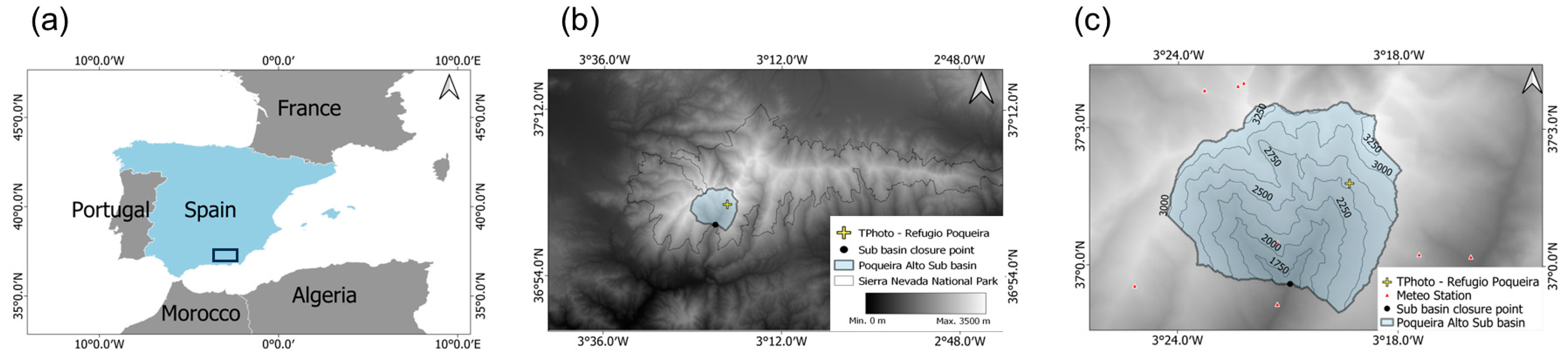
2.1. The Sierra Nevada Mountain Range
- −
- Plot scale—The Refugio Poqueira experimental site (Figure 1c, yellow cross). This area was selected to understand the connection between backscatter signals and snow dynamics. It is located at 2500 m a.s.l. and has been highly monitored since 2004, focusing on the microscale effects of snow ablation in Mediterranean mountains. The experimental site is equipped with a complete weather station (Table 1);
- −
- Catchment scale—The Poqueira Alto catchment (Figure 1c). This catchment was selected as a study site to connect wet-snow dynamics with streamflow response. It is a small catchment (54.91 km2) corresponding to the headwaters of the Poqueira River. With a mean elevation of 2513 m a.s.l., its hydrological response is totally driven by snow dynamics (Table 1).
2.2. Available Data
2.2.1. Meteorological Information
2.2.2. Proximal and Remote Sensing Observations
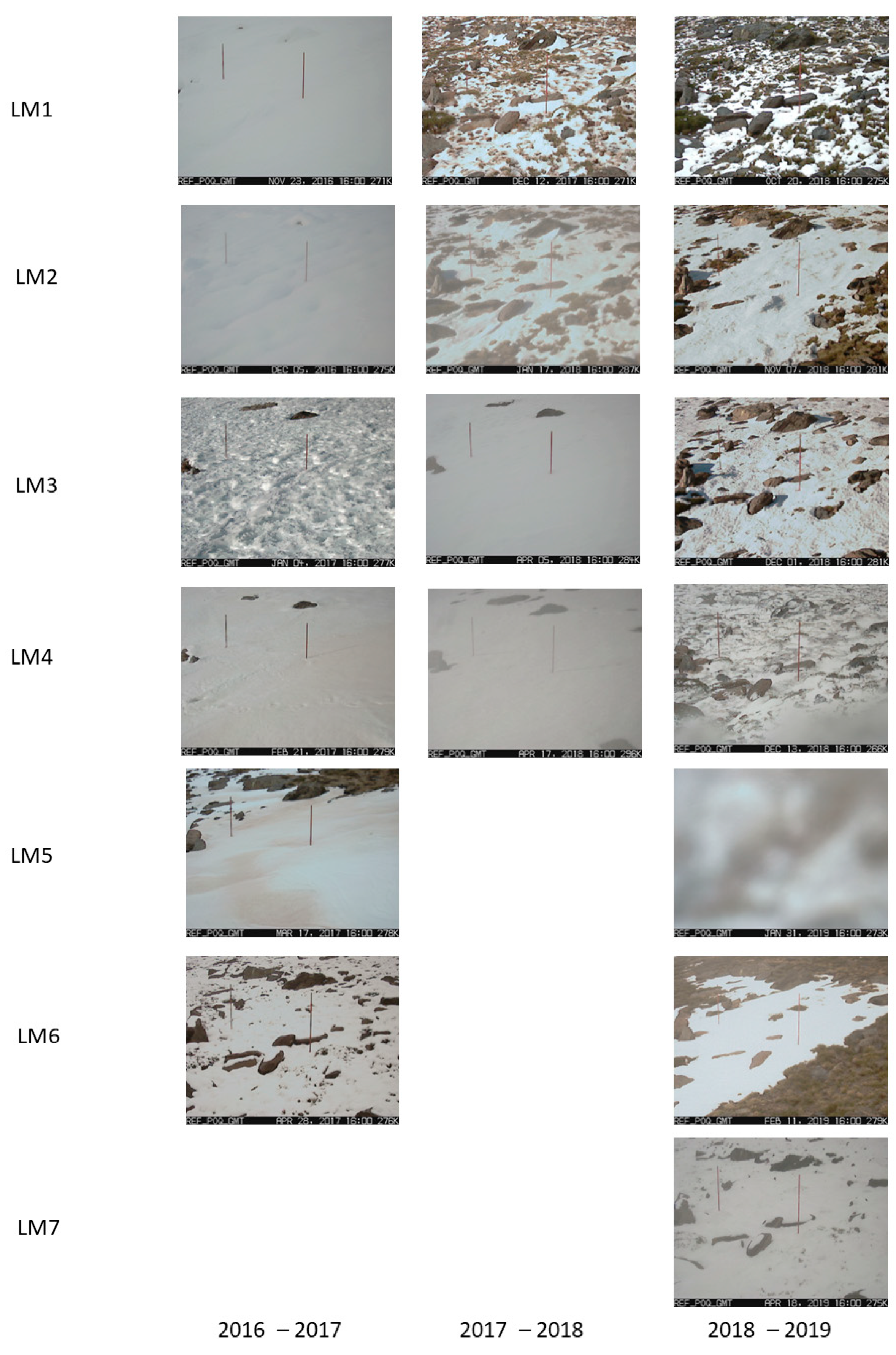
- Terrestrial photography
- Sentinel-1 SAR imagery
- Optical MODIS data: MOD10A2 Snow product
2.2.3. Streamflow Data
3. Methodology
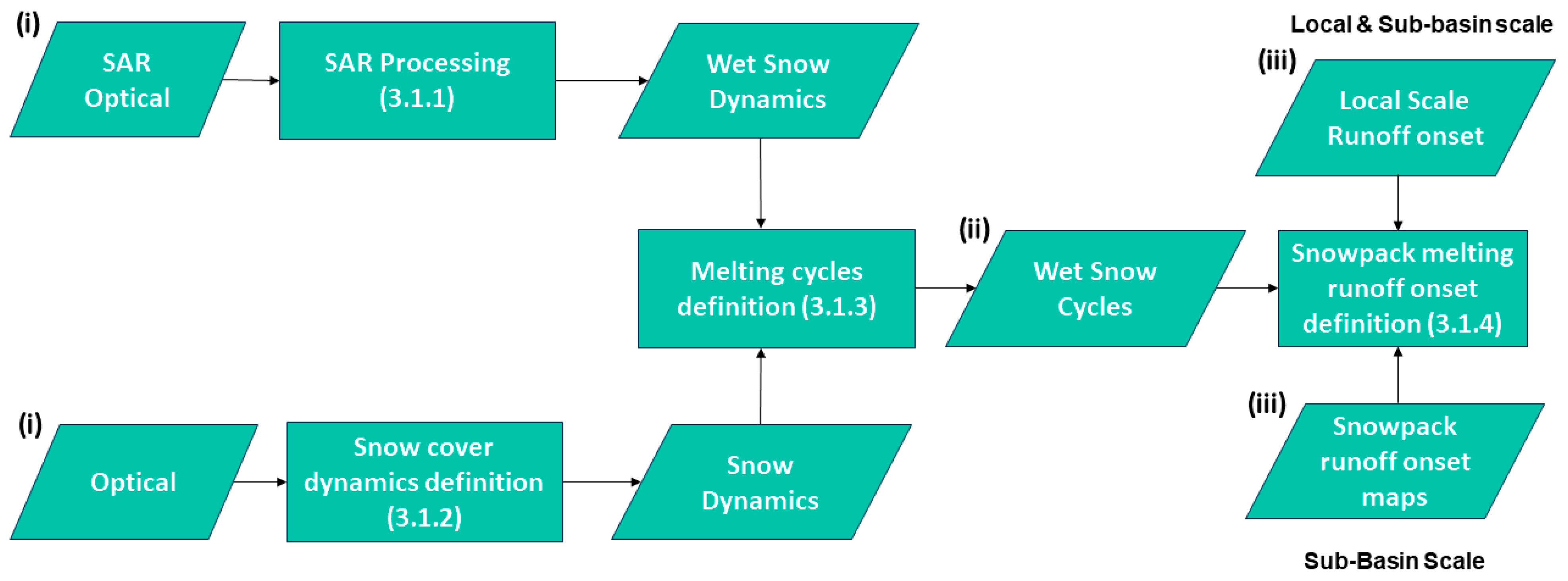
3.1. Definition of Snowpack Wet-Snow Dynamics
3.1.1. SAR Processing
- SAR image preprocessing
- Reference image selection
- Wet-snow threshold definition
- Cross-Evaluation
- Optical snow cover extension discrimination
3.1.2. Snow Cover Dynamics Definition
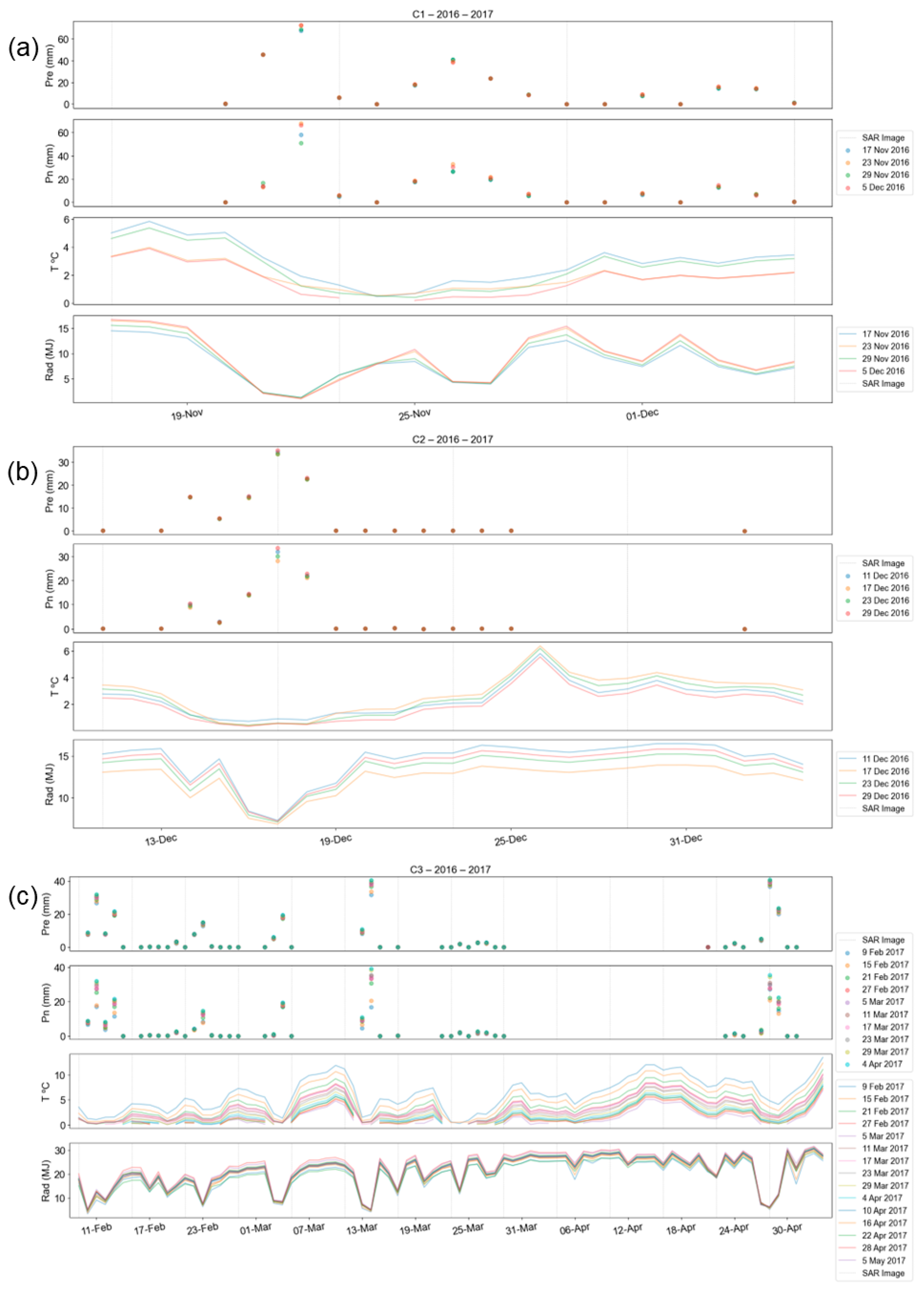
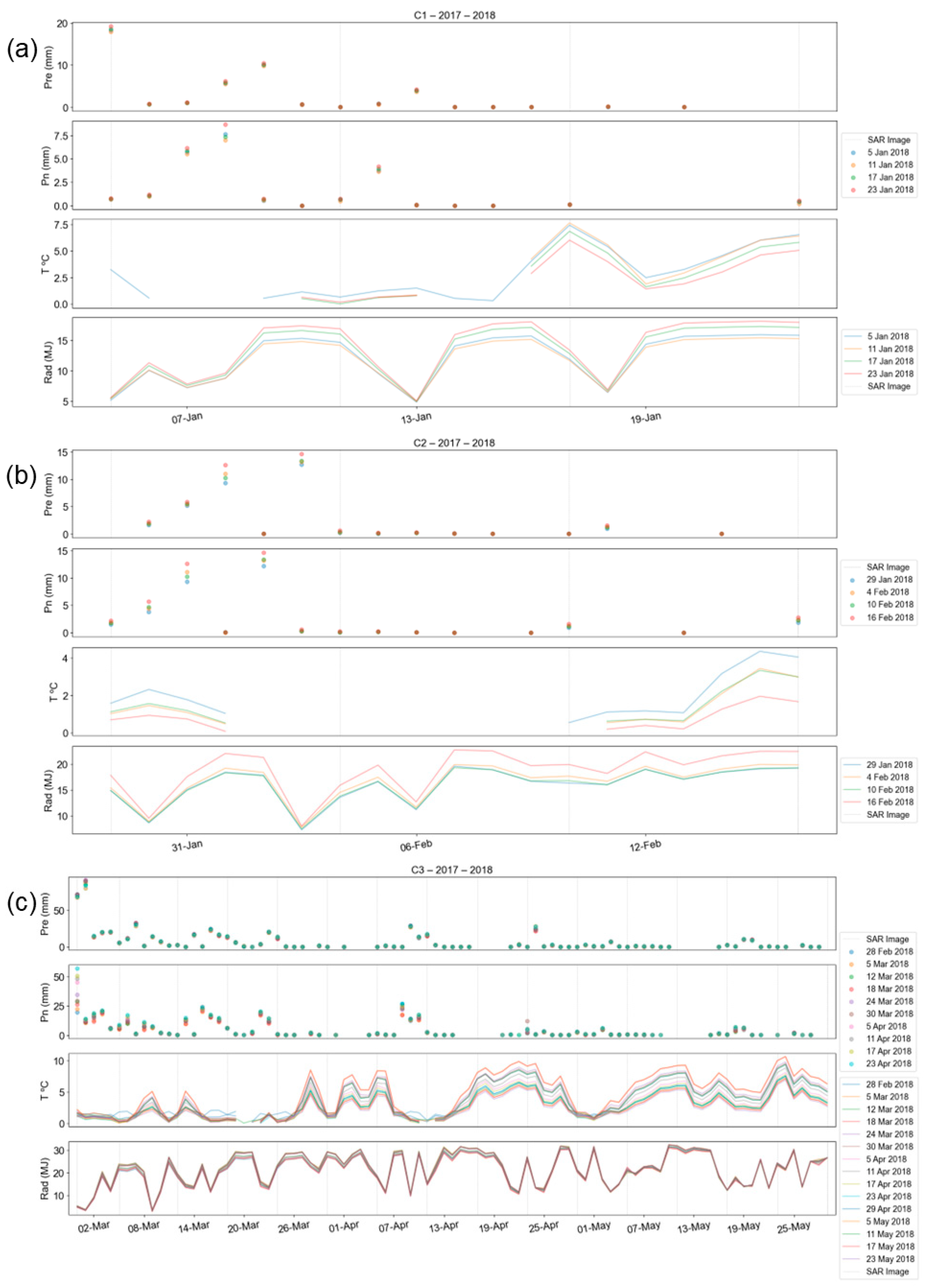
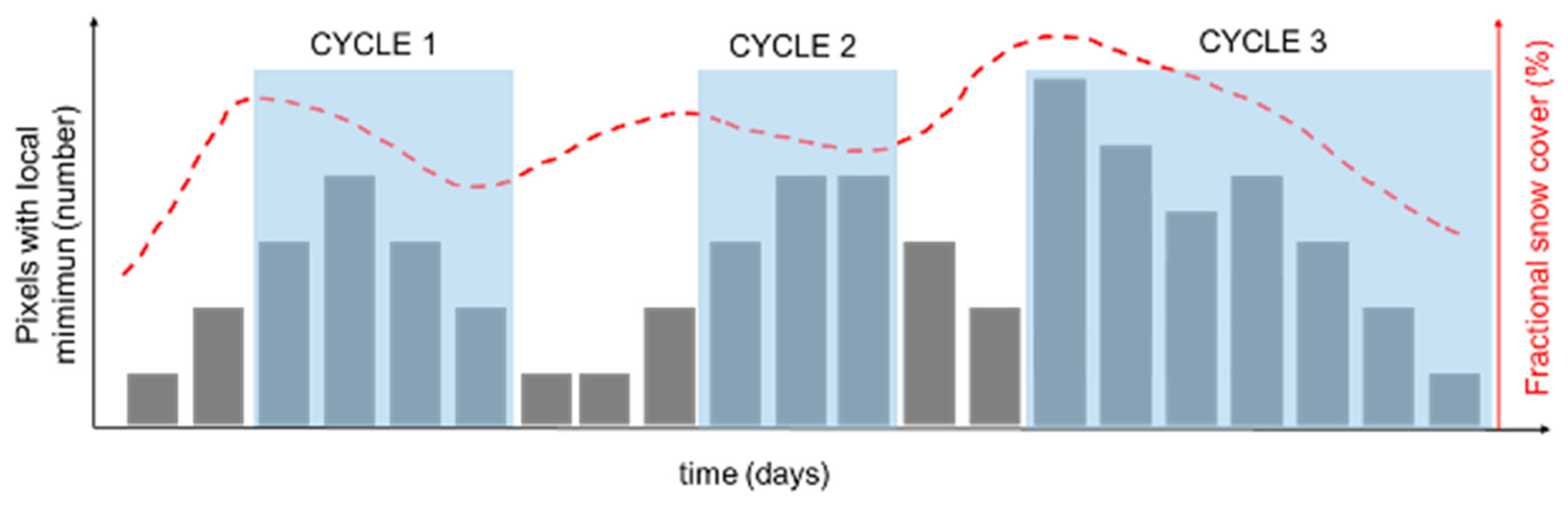
3.1.3. Melting Cycles Definition
3.1.4. Identification of the Relationship between Snowpack Melting and Runoff Onset
- Local Scale Runoff onset interpretation
- Snowpack runoff onset maps
3.2. Wet Snow–Streamflow Interaction
4. Results
4.1. Definition of Snowpack Wet-Snow Dynamics
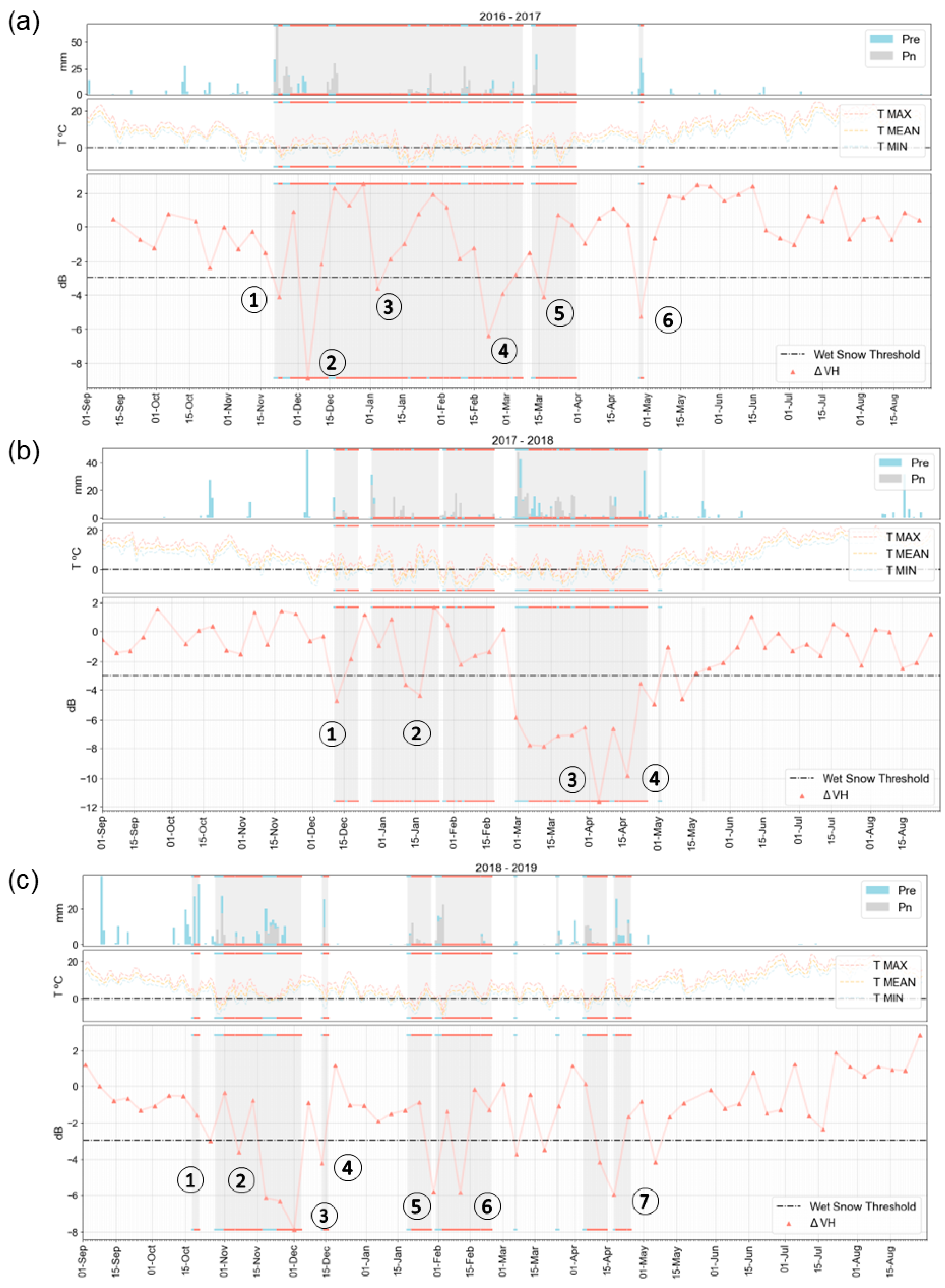
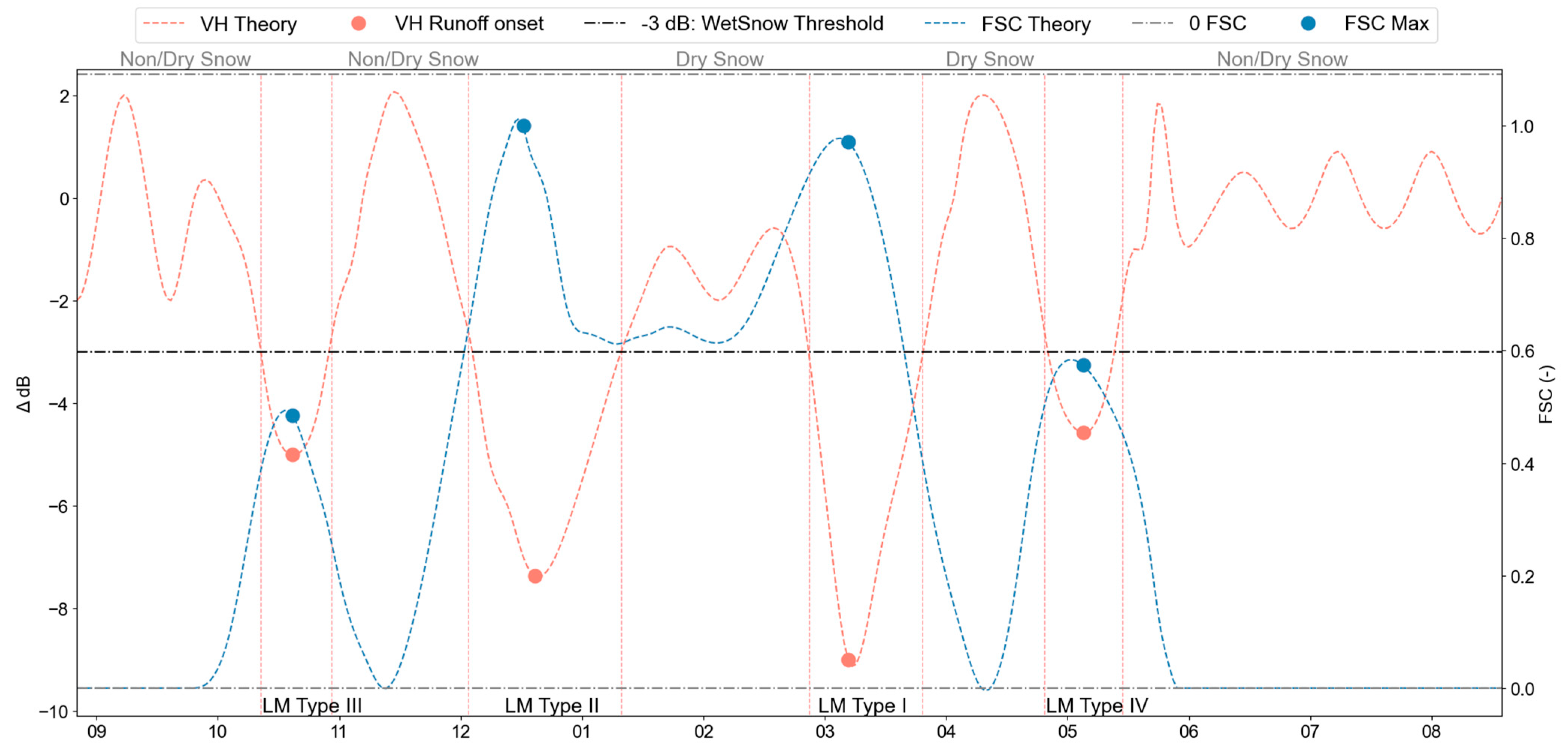
4.1.1. Local Scale: Backscatter Signal Understanding
- Local Minima Classification
- −
- Local Minimum Type I: the LM is found at the end of a well-developed snowpack. It is representative of long-lasting snow cycles, with a large amount of snow, resulting from a long accumulation phase, and it is associated with a very compact state of the snow with a high level of metamorphism. This LM is found in melting cycles described by depletion curve Type I in [3];
- −
- Local Minimum Type II: the LM is not unique in the snow cycle. It describes a quick melting period that is stopped by another snowfall or cold period that refreezes snow. This LM is found in melting cycles described by depletion curve Type II in [3];
- −
- Local Minimum Type III: the LM is unique within the melting cycle, that is, before and after this LM there is no snow. In addition, it takes place at the beginning of the snow season, when the energy exchange between the snowpack and the ground causes liquid water content to increase. This LM is found in melting cycles described by depletion curve Type III in [3];
- −
- Local Minimum Type IV: as in the previous case, the LM is singular, meaning that there is no snow before or after this particular LM. However, in this case, the minimum appears in sporadic snow cycles that occur during late winter or spring, and always after the main melting cycle. The LM is connected to a melting trigger by an increase in the temperature and incoming flux of shortwave radiation. This LM is found in melting cycles described by depletion curve IV in [3].
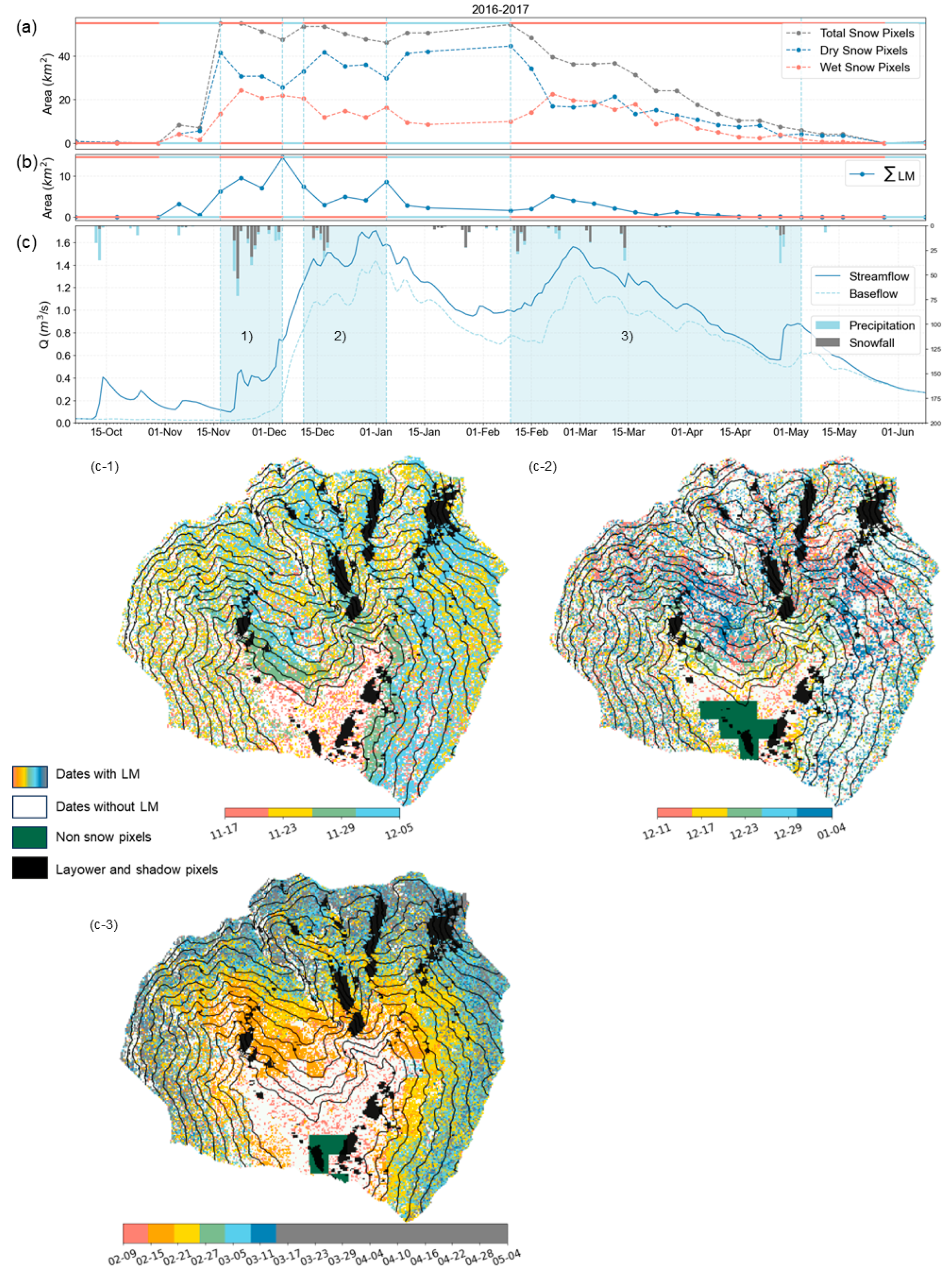
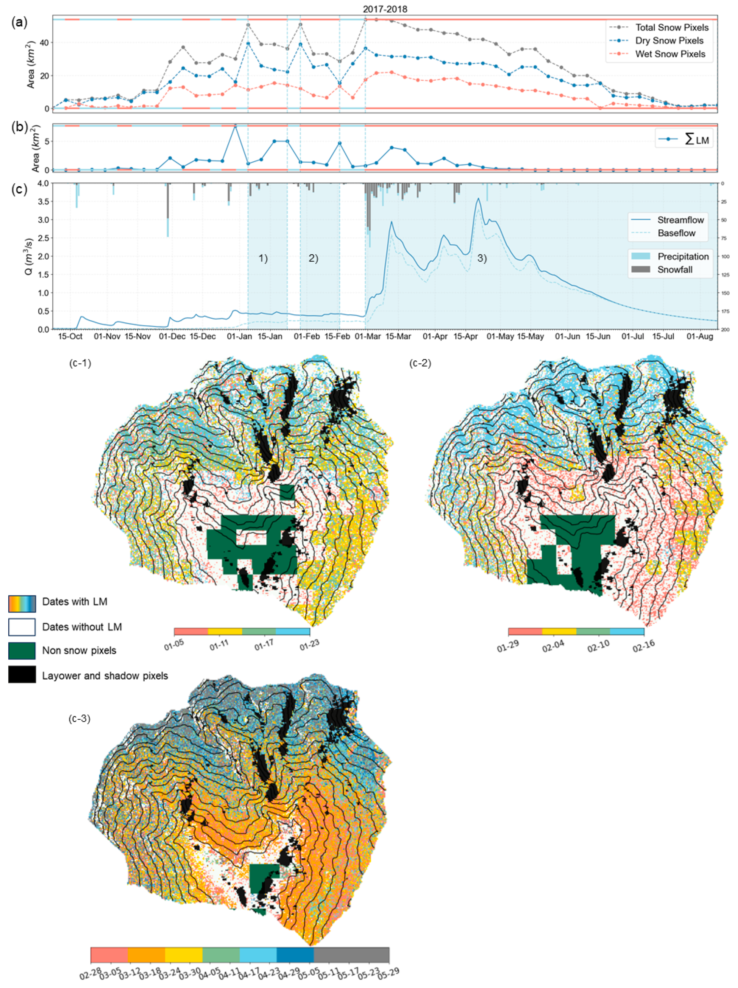
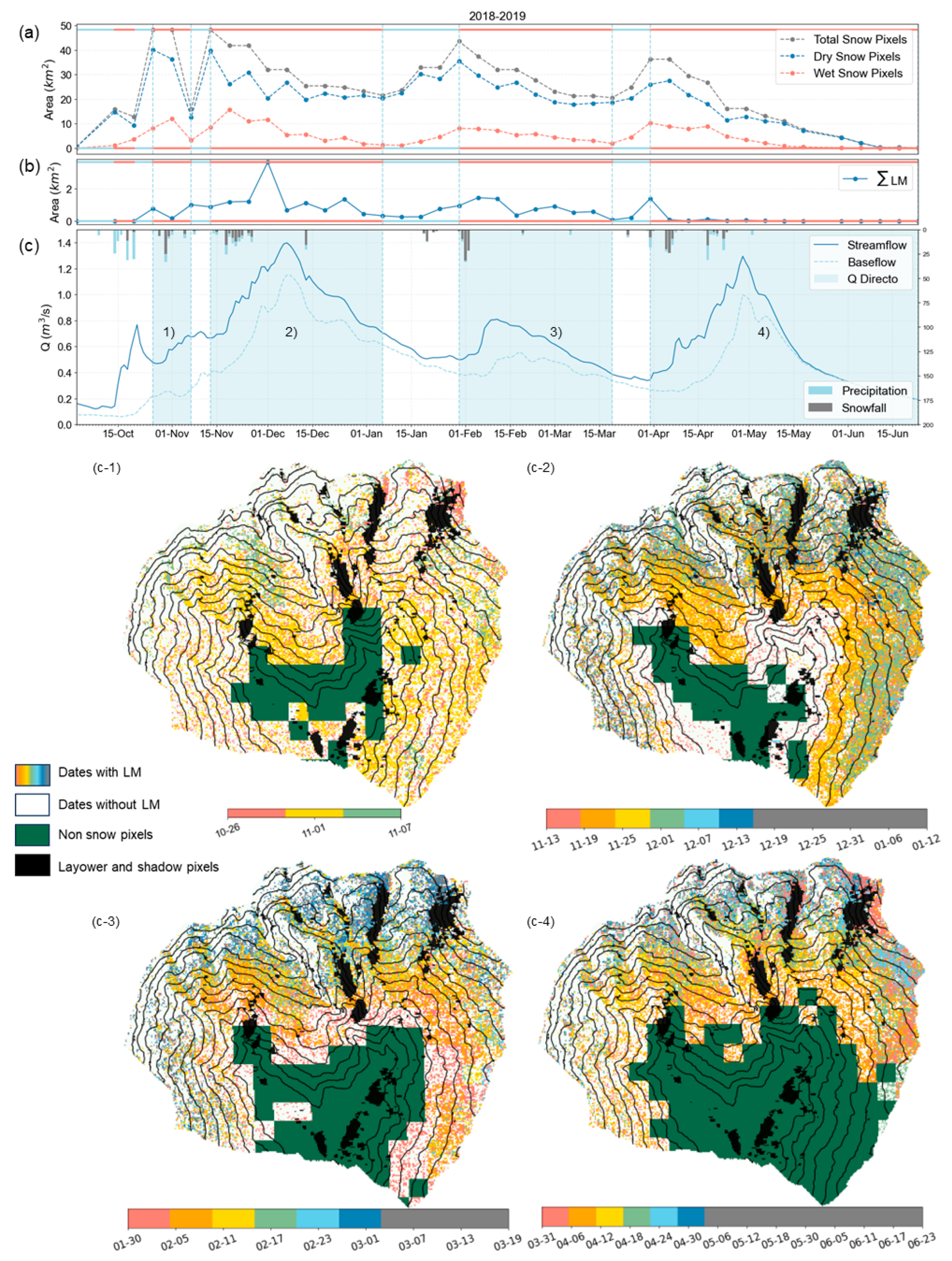
4.1.2. Catchment Scale: Melting Runoff Onset Maps
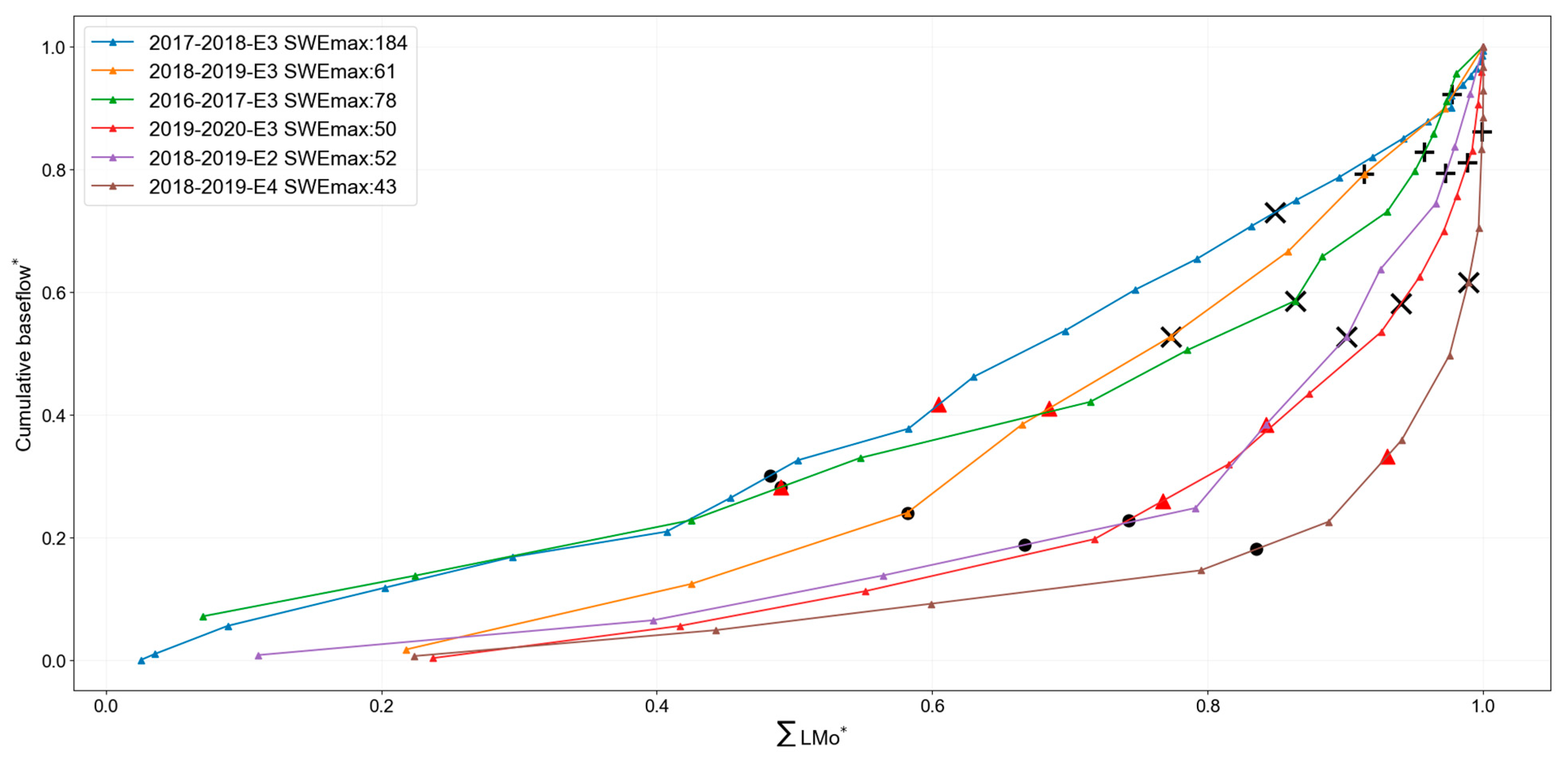
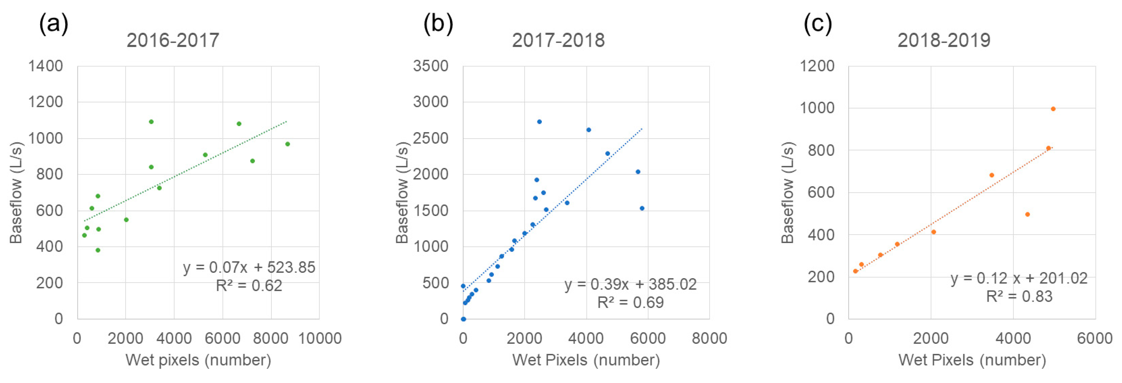
4.2. Wet Snow and Streamflow Interaction
- −
- Part 1 is represented by a linear and an almost horizontal function. Here, there is a high increase in the number of wet snow pixels with almost no change in baseflow response. Hence, this part reflects the delay observed between the beginning of the melting period and the actual response in the river;
- −
- Part 2 can be represented by a power function. In this case, there is an increasing pattern in both variables, which means that both processes, the melting and the baseflow response were occurring at the same time;
- −
- Part 3 follows again a linear function, but in this case, with a vertical pattern. Therefore, the behavior here is the opposite compared to Part 1, that is, we observe an increase in baseflow with limited contribution of wet snow pixels. Then, this part represents the time when almost no contribution from wet snow is happening but baseflow is still contributing to the streamflow.
5. Discussion
6. Conclusions
Author Contributions
Funding
Data Availability Statement
Acknowledgments
Conflicts of Interest
Appendix A
- Sensitivity Analysis

- Local Scale: Wet Snow Threshold definition

- Cross-Evaluation

| S1-S | S1-F | Acc | ||
|---|---|---|---|---|
| 5 March 2017 | LS-S | 0.66 | 0.34 | |
| LS-F | 0.27 | 0.73 | ||
| 0.69 | ||||
| 17 March 2017 | LS-S | 0.82 | 0.18 | |
| LS-F | 0.47 | 0.53 | ||
| 0.67 | ||||
| 10 April 2017 | LS-S | 0.28 | 0.72 | |
| LS-F | 0.06 | 0.94 | ||
| 0.84 | ||||
| 17 April 2018 | LS-S | 0.74 | 0.26 | |
| LS-F | 0.22 | 0.78 | ||
| 0.76 | ||||
| 11 May 2018 | LS-S | 0.63 | 0.37 | |
| LS-F | 0.09 | 0.91 | ||
| 0.77 | ||||
| 6 May 2019 | LS-S | 0.31 | 0.69 | |
| LS-F | 0.06 | 0.94 | ||
| 0.84 | ||||
| 18 June 2019 | LS-S | 0.17 | 0.83 | |
| LS-F | 0.04 | 0.96 | ||
| 0.93 | ||||
| Average | 0.79 |
- Local Scale: Backscatter signal understanding—Terrestrial images

- Catchment Scale: Analysis of the impact of meteorological variables on LMo


References
- Allan, R.P.; Barlow, M.; Byrne, M.P.; Cherchi, A.; Douville, H.; Fowler, H.J.; Gan, T.Y.; Pendergrass, A.G.; Rosenfeld, D.; Swann, A.L.S.; et al. Advances in Understanding Large-Scale Responses of the Water Cycle to Climate Change. Ann. N. Y. Acad. Sci. 2020, 1472, 49–75. [Google Scholar] [CrossRef] [PubMed]
- Polo, M.J.; Pimentel, R.; Gascoin, S.; Notarnicola, C. Mountain Hydrology in the Mediterranean Region. In Water Resources in the Mediterranean Region; Elsevier: Amsterdam, The Netherlands, 2020; pp. 51–75. [Google Scholar] [CrossRef]
- Pimentel, R.; Herrero, J.; Polo, M.J. Subgrid Parameterization of Snow Distribution at a Mediterranean Site Using Terrestrial Photography. Hydrol. Earth Syst. Sci. 2017, 21, 805–820. [Google Scholar] [CrossRef]
- Pimentel, R.; Herrero, J.; Polo, M. Quantifying Snow Cover Distribution in Semiarid Regions Combining Satellite and Terrestrial Imagery. Remote Sens. 2017, 9, 995. [Google Scholar] [CrossRef]
- Fayad, A.; Gascoin, S.; Faour, G.; Fanise, P.; Drapeau, L.; Somma, J.; Fadel, A.; Al Bitar, A.; Escadafal, R. Snow Observations in Mount Lebanon (2011–2016). Earth Syst. Sci. Data 2017, 9, 573–587. [Google Scholar] [CrossRef]
- Herrero, J.; Polo, M.J. Evaposublimation from the Snow in the Mediterranean Mountains of Sierra Nevada (Spain). Cryosphere 2016, 10, 2981–2998. [Google Scholar] [CrossRef]
- Thakur, P.K.; Garg, V.; Nikam, B.R.; Singh, S.; Chouksey, A.; Dhote, P.R.; Aggarwal, S.P.; Chauhan, P.; Kumar, A.S. Snow cover and glacier dynamics study using C-and L-band SAR datasets in parts of North West Himalaya. Int. Arch. Photogramm. Remote Sens. Spat. Inf. Sci. 2018, 42, 375–382. [Google Scholar] [CrossRef]
- Contreras, E.; Herrero, J.; Crochemore, L.; Aguilar, C.; Polo, M.J. Seasonal Climate Forecast Skill Assessment for the Management of Water Resources in a Run of River Hydropower System in the Poqueira River (Southern Spain). Water 2020, 12, 2119. [Google Scholar] [CrossRef]
- Gray, D.; McKay, G. The Handbook of Snow: Principles, Processes, Management & Use; Pergamon Press: Toronto, QC, Canada, 1981. [Google Scholar]
- DeWalle, D.R.; Rango, A. Principles of Snow Hydrology; Cambridge University Press: Cambridge, UK, 2008; ISBN 9780521823623. [Google Scholar]
- House, A. Corrigendum to: Physical Hydrology By S. Lawrence Dingman [Hydrological Sciences Journal, (2015), 643]. Hydrol. Sci. J. 2015, 60. [Google Scholar] [CrossRef]
- Elder, K.; Dozier, J.; Michaelsen, J. Snow Accumulation and Distribution in an Alpine Watershed. Water Resour. Res. 1991, 27, 1541–1552. [Google Scholar] [CrossRef]
- Egli, L.; Jonas, T.; Meister, R. Comparison of Different Automatic Methods for Estimating Snow Water Equivalent. Cold Reg. Sci. Technol. 2009, 57, 107–115. [Google Scholar] [CrossRef]
- Domine, F. Physical Properties of Snow. In Encyclopedia of Snow, Ice and Glaciers; Encyclopedia of Earth Sciences Series; Springer: Dordrecht, The Netherlands, 2011; Volume 3. [Google Scholar]
- Colbeck, S.C. An Overview of Seasonal Snow Metamorphism. Rev. Geophys. 1982, 20, 45–61. [Google Scholar] [CrossRef]
- Kinar, N.J.; Pomeroy, J.W. Measurement of the Physical Properties of the Snowpack. Rev. Geophys. 2015, 53, 481–544. [Google Scholar] [CrossRef]
- Pirazzini, R.; Leppänen, L.; Picard, G.; Lopez-Moreno, J.I.; Marty, C.; Macelloni, G.; Kontu, A.; von Lerber, A.; Tanis, C.M.; Schneebeli, M.; et al. European In-Situ Snow Measurements: Practices and Purposes. Sensors 2018, 18, 2016. [Google Scholar] [CrossRef] [PubMed]
- Yuan, S.; Zheng, J.; Zhang, L.; Dong, R.; Xing, Y.; She, Y.; Fu, H.; Cheung, R.C.C. Melting Glacier: A 37-Year (1984–2020) High-Resolution Glacier-Cover Record of MT. Kilimanjaro. In Proceedings of the IGARSS 2022—2022 IEEE International Geoscience and Remote Sensing Symposium, Kuala Lumpur, Malaysia, 17–22 July 2022. [Google Scholar]
- Snapir, B.; Momblanch, A.; Jain, S.K.; Waine, T.W.; Holman, I.P. A Method for Monthly Mapping of Wet and Dry Snow Using Sentinel-1 and MODIS: Application to a Himalayan River Basin. Int. J. Appl. Earth Obs. Geoinf. 2019, 74, 222–230. [Google Scholar] [CrossRef]
- Arslan, A.N.; Akyürek, Z. Special Issue on Remote Sensing of Snow and Its Applications. Geosciences 2019, 9, 277. [Google Scholar] [CrossRef]
- Helbig, N.; Schirmer, M.; Magnusson, J.; Mäder, F.; Van Herwijnen, A.; Quéno, L.; Bühler, Y.; Deems, J.S.; Gascoin, S. A Seasonal Algorithm of the Snow-Covered Area Fraction for Mountainous Terrain. Cryosphere 2021, 15, 4607–4624. [Google Scholar] [CrossRef]
- Riggs, G.; Hall, D. MODIS Snow Products Collection 6 User Guide; National Snow and Ice Data Center: Boulder, CO, USA, 2016. [Google Scholar]
- Zhang, P.; Shi, X.; Khan, S.U.; Ferreira, B.; Portela, B.; Oliveira, T.; Borges, G.; Domingos, H.; Leitão, J.; Mohottige, I.P.; et al. IEEE Draft Standard for Spectrum Characterization and Occupancy Sensing. IEEE Access 2019, 9, 11–13. [Google Scholar]
- Bair, E.H.; Rittger, K.; Skiles, S.M.K.; Dozier, J. An Examination of Snow Albedo Estimates From MODIS and Their Impact on Snow Water Equivalent Reconstruction. Water Resour. Res. 2019, 55, 7826–7842. [Google Scholar] [CrossRef]
- Pimentel, R.; Aguilar, C.; Herrero, J.; Pérez-Palazón, M.J.; Polo, M.J. Comparison between Snow Albedo Obtained from Landsat TM, ETM+ Imagery and the SPOT VEGETATION Albedo Product in a Mediterranean Mountainous Site. Hydrology 2016, 3, 10. [Google Scholar] [CrossRef]
- Painter, T.H.; Rittger, K.; McKenzie, C.; Slaughter, P.; Davis, R.E.; Dozier, J. Retrieval of Subpixel Snow Covered Area, Grain Size, and Albedo from MODIS. Remote Sens. Environ. 2009, 113, 868–879. [Google Scholar] [CrossRef]
- Vargel, C.; Royer, A.; St-Jean-Rondeau, O.; Picard, G.; Roy, A.; Sasseville, V.; Langlois, A. Arctic and Subarctic Snow Microstructure Analysis for Microwave Brightness Temperature Simulations. Remote Sens. Environ. 2020, 242, 111754. [Google Scholar] [CrossRef]
- Tsai, Y.L.S.; Dietz, A.; Oppelt, N.; Kuenzer, C. Wet and Dry Snow Detection Using Sentinel-1 SAR Data for Mountainous Areas with a Machine Learning Technique. Remote Sens. 2019, 11, 895. [Google Scholar] [CrossRef]
- Hafner, E.D.; Techel, F.; Leinss, S.; Bühler, Y. Mapping Avalanches with Satellites-Evaluation of Performance and Completeness. Cryosphere 2021, 15, 983–1004. [Google Scholar] [CrossRef]
- Sugiura, K.; Nagai, S.; Nakai, T.; Suzuki, R. Application of Time-Lapse Digital Imagery for Ground-Truth Verification of Satellite Indices in the Boreal Forests of Alaska. Polar Sci. 2013, 7, 149–161. [Google Scholar] [CrossRef]
- Garvelmann, J.; Pohl, S.; Weiler, M. From Observation to the Quantification of Snow Processes with a Time-Lapse Camera Network. Hydrol. Earth Syst. Sci. 2013, 17, 1415–1429. [Google Scholar] [CrossRef]
- Fassnacht, S.R.; Stednick, J.D.; Deems, J.S.; Corrao, M.V. Metrics for Assessing Snow Surface Roughness from Digital Imagery. Water Resour. Res. 2009, 45, W00D31. [Google Scholar] [CrossRef]
- Corripio, J.G. Snow Surface Albedo Estimation Using Terrestrial Photography. Int. J. Remote Sens. 2004, 25, 5705–5729. [Google Scholar] [CrossRef]
- Nagler, T.; Rott, H.; Ripper, E.; Bippus, G.; Hetzenecker, M. Advancements for Snowmelt Monitoring by Means of Sentinel-1 SAR. Remote Sens. 2016, 8, 348. [Google Scholar] [CrossRef]
- Karbou, F.; James, G.; Fructus, M.; Marti, F. On the Evaluation of the SAR-Based Copernicus Snow Products in the French Alps. Geosciences 2022, 12, 420. [Google Scholar] [CrossRef]
- Lievens, H.; Demuzere, M.; Marshall, H.P.; Reichle, R.H.; Brucker, L.; Brangers, I.; de Rosnay, P.; Dumont, M.; Girotto, M.; Immerzeel, W.W.; et al. Snow Depth Variability in the Northern Hemisphere Mountains Observed from Space. Nat. Commun. 2019, 10, 4629. [Google Scholar] [CrossRef]
- Santi, E.; De Gregorio, L.; Pettinato, S.; Cuozzo, G.; Jacob, A.; Notarnicola, C.; Gunther, D.; Strasser, U.; Cigna, F.; Tapete, D.; et al. On the Use of COSMO-SkyMed X-Band SAR for Estimating Snow Water Equivalent in Alpine Areas: A Retrieval Approach Based on Machine Learning and Snow Models. IEEE Trans. Geosci. Remote Sens. 2022, 60, 4305419. [Google Scholar] [CrossRef]
- Xiao, X.; Liang, S.; He, T.; Wu, D.; Pei, C.; Gong, J. Estimating Fractional Snow Cover from Passive Microwave Brightness Temperature Data Using MODIS Snow Cover Product over North America. Cryosphere 2021, 15, 835–861. [Google Scholar] [CrossRef]
- Luojus, K.; Pulliainen, J.; Takala, M.; Lemmetyinen, J.; Moisander, M. GlobSnow v3.0 Snow Water Equivalent (SWE). Available online: https://doi.pangaea.de/10.1594/PANGAEA.911944 (accessed on 10 November 2023).
- Jia, A.; Wang, D.; Liang, S.; Peng, J.; Yu, Y. Improved Cloudy-Sky Snow Albedo Estimates Using Passive Microwave and VIIRS Data. ISPRS J. Photogramm. Remote Sens. 2023, 196, 340–355. [Google Scholar] [CrossRef]
- Koike, T.; Suhama, T. Passive-Microwave Remote Sensing of Snow. Ann. Glaciol. 1993, 18, 305–308. [Google Scholar] [CrossRef]
- Ulaby, F.T.; Stiles, W.H.; Dellwig, L.F.; Hanson, B.C. Experiments on the Radar Backscatter of Snow. IEEE Trans. Geosci. Electron. 1977, 15, 185–189. [Google Scholar] [CrossRef]
- Marin, C.; Bertoldi, G.; Premier, V.; Callegari, M.; Brida, C.; Hürkamp, K.; Tschiersch, J.; Zebisch, M.; Notarnicola, C. Use of Sentinel-1 Radar Observations to Evaluate Snowmelt Dynamics in Alpine Regions. Cryosphere 2020, 14, 935–956. [Google Scholar] [CrossRef]
- Antropova, Y.K.; Komarov, A.S.; Richardson, M.; Millard, K.; Smith, K. Detection of Wet Snow in the Arctic Tundra from Time-Series Fully-Polarimetric RADARSAT-2 Images. Remote Sens. Environ. 2022, 283, 113305. [Google Scholar] [CrossRef]
- Darychuk, S.E.; Shea, J.M.; Menounos, B.; Chesnokova, A.; Jost, G.; Weber, F. Snowmelt Characterization from Optical and Synthetic-Aperture Radar Observations in the La Joie Basin, British Columbia. Cryosphere 2023, 17, 1457–1473. [Google Scholar] [CrossRef]
- Torres, R.; Snoeij, P.; Geudtner, D.; Bibby, D.; Davidson, M.; Attema, E.; Potin, P.; Rommen, B.Ö.; Floury, N.; Brown, M.; et al. GMES Sentinel-1 Mission. Remote Sens. Environ. 2012, 120, 9–24. [Google Scholar] [CrossRef]
- Nagler, T.; Schwaizer, G.; Ossowska, J.; Rott, H.; Small, D. Towards an Advanced Pan-European Snow Cover Product from Sentinel-1 SAR and Sentinel-3 SLSTR. In Proceedings of the EGU General Assembly 2018, Vienna, Austria, 8–13 April 2018; Volume 20. [Google Scholar]
- Veyssière, G.; Karbou, F.; Morin, S.; Lafaysse, M.; Vionnet, V. Evaluation of Sub-Kilometric Numerical Simulations of C-Band Radar Backscatter over the French Alps against Sentinel-1 Observations. Remote Sens. 2019, 11, 8. [Google Scholar] [CrossRef]
- Heilig, A.; Wendleder, A.; Schmitt, A.; Mayer, C. Discriminating Wet Snow and Firn for Alpine Glaciers Using Sentinel-1 Data: A Case Study at Rofental, Austria. Geosciences 2019, 9, 69. [Google Scholar] [CrossRef]
- Ramage, J.M.; McKenney, R.A.; Thorson, B.; Maltais, P.; Kopczynski, S.E. Relationship between Passive Microwave-Derived Snowmelt and Surface-Measured Discharge, Wheaton River, Yukon Territory, Canada. Hydrol. Process. 2006, 20, 689–704. [Google Scholar] [CrossRef]
- Hall, D.K.; Foster, J.L.; DiGirolamo, N.E.; Riggs, G.A. Snow Cover, Snowmelt Timing and Stream Power in the Wind River Range, Wyoming. Geomorphology 2012, 137, 87–93. [Google Scholar] [CrossRef]
- Godsey, S.E.; Kirchner, J.W. Dynamic, Discontinuous Stream Networks: Hydrologically Driven Variations in Active Drainage Density, Flowing Channels and Stream Order. Hydrol. Process. 2014, 28, 5791–5803. [Google Scholar] [CrossRef]
- Uzun, S.; Tanir, T.; Coelho, G.d.A.; de Souza de Lima, A.; Cassalho, F.; Ferreira, C.M. Changes in Snowmelt Runoff Timing in the Contiguous United States. Hydrol. Process. 2021, 35, e14430. [Google Scholar] [CrossRef]
- Li, S.; Liu, M.; Adam, J.C.; Pi, H.; Su, F.; Li, D.; Liu, Z.; Yao, Z. Contribution of Snow-Melt Water to the Streamflow over the Three-River Headwater Region, China. Remote Sens. 2021, 13, 1585. [Google Scholar] [CrossRef]
- Blankinship, J.C.; Meadows, M.W.; Lucas, R.G.; Hart, S.C. Snowmelt Timing Alters Shallow but Not Deep Soil Moisture in the Sierra Nevada. Water Resour. Res. 2014, 50, 1448–1456. [Google Scholar] [CrossRef]
- McNamara, J.P.; Chandler, D.; Seyfried, M.; Achet, S. Soil Moisture States, Lateral Flow, and Streamflow Generation in a Semi-Arid, Snowmelt-Driven Catchment. Hydrol. Process. 2005, 19, 4023–4038. [Google Scholar] [CrossRef]
- Chen, X.; Tang, G.; Chen, T.; Niu, X. An Assessment of the Impacts of Snowmelt Rate and Continuity Shifts on Streamflow Dynamics in Three Alpine Watersheds in the Western U.S. Water 2022, 14, 1095. [Google Scholar] [CrossRef]
- Rondeau-Genesse, G.; Trudel, M.; Leconte, R. Monitoring Snow Wetness in an Alpine Basin Using Combined C-Band SAR and MODIS Data. Remote Sens. Environ. 2016, 183, 304–317. [Google Scholar] [CrossRef]
- Tramblay, Y.; Koutroulis, A.; Samaniego, L.; Vicente-Serrano, S.M.; Volaire, F.; Boone, A.; Le Page, M.; Llasat, M.C.; Albergel, C.; Burak, S.; et al. Challenges for Drought Assessment in the Mediterranean Region under Future Climate Scenarios. Earth-Sci. Rev. 2020, 210, 103348. [Google Scholar] [CrossRef]
- Pimentel, R.; Herrero, J.; Zeng, Y.; Su, Z.; Polo, M.J. Study of Snow Dynamics at Subgrid Scale in Semiarid Environments Combining Terrestrial Photography and Data Assimilation Techniques. J. Hydrometeorol. 2015, 16, 563–578. [Google Scholar] [CrossRef]
- Guiot, A.; Karbou, F.; James, G.; Durand, P. Insights into Segmentation Methods Applied to Remote Sensing SAR Images for Wet Snow Detection. Geosciences 2023, 13, 193. [Google Scholar] [CrossRef]
- Pérez-Palazón, M.J.; Pimentel, R.; Polo, M.J. Climate Trends Impact on the Snowfall Regime in Mediterranean Mountain Areas: Future Scenario Assessment in Sierra Nevada (Spain). Water 2018, 10, 720. [Google Scholar] [CrossRef]
- Herrero, J.; Polo, M.J.; Moñino, A.; Losada, M.A. An Energy Balance Snowmelt Model in a Mediterranean Site. J. Hydrol. 2009, 371, 98–107. [Google Scholar] [CrossRef]
- Polo, M.J.; Herrero, J.; Pimentel, R.; Pérez-Palazón, M.J. The Guadalfeo Monitoring Network (Sierra Nevada, Spain): 14 Years of Measurements to Understand the Complexity of Snow Dynamics in Semiarid Regions. Earth Syst. Sci. Data 2019, 11, 393–407. [Google Scholar] [CrossRef]
- Aguilar, C.; Herrero, J.; Millares, A.; Losada, M.A.; Polo, M.J. Meteomap: Generation of Meteorological Variables for Distribuited Physically-Based Hydrological Modeling. In Proceedings of the 11th International Conference on Hydroinformatics, New York, NY, USA, 17–21 August 2014. [Google Scholar]
- Herrero, J.; Aguilar, C.; Polo, M.J.; Losada, M.Á. Mapping of Meteorological Varaibles for Runoff Generation Forecast in Distributed Hydrological Modeling. In Proceedings of the Hydraulic Measurements & Experimental Methods Conference (ASCE/IAHR), Lake Placid, NY, USA, 10–12 September 2007; pp. 606–611. [Google Scholar]
- Aguilar, C.; Herrero, J.; Polo, M.J. Topographic Effects on Solar Radiation Distribution in Mountainous Watersheds and Their Influence on Reference Evapotranspiration Estimates at Watershed Scale. Hydrol. Earth Syst. Sci. 2010, 14, 2479–2494. [Google Scholar] [CrossRef]
- Mätzler, C. Applications of the Interaction of Microwaves with the Natural Snow Cover. Remote Sens. Rev. 1987, 2, 259–387. [Google Scholar] [CrossRef]
- Strozzi, T.; Wiesmann, A.; Mätzler, C. Active Microwave Signatures of Snow Covers at 5.3 and 35 GHz. Radio Sci. 1997, 32, 479–495. [Google Scholar] [CrossRef]
- Hall, D.K.; Riggs, G.A. Accuracy Assessment of the MODIS Snow Products. Hydrol. Process. 2007, 21, 1534–1547. [Google Scholar] [CrossRef]
- Coll, J.; Li, X. Comprehensive Accuracy Assessment of MODIS Daily Snow Cover Products and Gap Filling Methods. ISPRS J. Photogramm. Remote Sens. 2018, 144, 435–452. [Google Scholar] [CrossRef]
- Notarnicola, C.; Duguay, M.; Moelg, N.; Schellenberger, T.; Tetzlaff, A.; Monsorno, R.; Costa, A.; Steurer, C.; Zebisch, M. Snow Cover Maps from MODIS Images at 250 m Resolution, Part 2: Validation. Remote Sens. 2013, 5, 1568–1587. [Google Scholar] [CrossRef]
- Parajka, J.; Holko, L.; Kostka, Z.; Blöschl, G. MODIS Snow Cover Mapping Accuracy in a Small Mountain Catchment—Comparison between Open and Forest Sites. Hydrol. Earth Syst. Sci. 2012, 16, 2365–2377. [Google Scholar] [CrossRef]
- Penman, H.L. Natural Evaporation from Open Water, Hare Soil and Grass. Proc. R. Soc. Lond. A Math. Phys. Sci. 1948, 193, 120–145. [Google Scholar] [CrossRef]
- Monteith, J.L.; Szeicz, G.; Yabuki, K. Crop Photosynthesis and the Flux of Carbon Dioxide Below the Canopy. J. Appl. Ecol. 1964, 1, 321. [Google Scholar] [CrossRef]
- Heber Green, W.; Ampt, G.A. Studies on Soil Phyics. J. Agric. Sci. 1911, 4, 1–24. [Google Scholar] [CrossRef]
- Millares, A.; Polo, M.J.; Losada, M.A. The Hydrological Response of Baseflow in Fractured Mountain Areas. Hydrol. Earth Syst. Sci. 2009, 13, 1261–1271. [Google Scholar] [CrossRef]
- Pastén-Zapata, E.; Pimentel, R.; Royer-Gaspard, P.; Sonnenborg, T.O.; Aparicio-Ibañez, J.; Lemoine, A.; Pérez-Palazón, M.J.; Schneider, R.; Photiadou, C.; Thirel, G.; et al. The Effect of Weighting Hydrological Projections Based on the Robustness of Hydrological Models under a Changing Climate. J. Hydrol. Reg. Stud. 2022, 41, 101113. [Google Scholar] [CrossRef]
- Nagler, T.; Rott, H. Snow Classification Algorithm for ENVISAT ASAR. In Proceedings of the 2004 Envisat & ERS Symposium (ESA SP-572), Salzburg, Austria, 6–10 September 2004. [Google Scholar]
- Nagler, T.; Rott, H. Retrieval of Wet Snow by Means of Multitemporal SAR Data. IEEE Trans. Geosci. Remote Sens. 2000, 38, 754–765. [Google Scholar] [CrossRef]
- Ulaby, F.; Long, D. Microwave Radar and Radiometric Remote Sensing; University of Michigan Press: Ann Arbor, MI, USA, 2014. [Google Scholar]
- He, G.; Feng, X.; Xiao, P.; Xia, Z.; Wang, Z.; Chen, H.; Li, H.; Guo, J. Dry and Wet Snow Cover Mapping in Mountain Areas Using SAR and Optical Remote Sensing Data. IEEE J. Sel. Top. Appl. Earth Obs. Remote Sens. 2017, 10, 2673409. [Google Scholar] [CrossRef]
- Schellenberger, T.; Ventura, B.; Zebisch, M.; Notarnicola, C. Wet Snow Cover Mapping Algorithm Based on Multitemporal COSMO-SkyMed X-Band SAR Images. IEEE J. Sel. Top. Appl. Earth Obs. Remote Sens. 2012, 5, 2190720. [Google Scholar] [CrossRef]
- Gorelick, N.; Hancher, M.; Dixon, M.; Ilyushchenko, S.; Thau, D.; Moore, R. Google Earth Engine: Planetary-Scale Geospatial Analysis for Everyone. Remote Sens. Environ. 2017, 202, 18–27. [Google Scholar] [CrossRef]
- Buchelt, S.; Skov, K.; Rasmussen, K.K.; Ullmann, T. Sentinel-1 Time Series for Mapping Snow Cover Depletion and Timing of Snowmelt in Arctic Periglacial Environments: Case Study from Zackenberg and Kobbefjord, Greenland. Cryosphere 2022, 16, 625–646. [Google Scholar] [CrossRef]
- Ulaby, F.T.; Abdelrazik, M.; Stiles, W.H. Snowcover Influence on Backscattering from Terrain. IEEE Trans. Geosci. Remote Sens. 1984, GE-22, 126–133. [Google Scholar] [CrossRef]
- Linlor, W.I. Permittivity and Attenuation of Wet Snow between 4 and 12 GHz. J. Appl. Phys. 1980, 51, 2811–2816. [Google Scholar] [CrossRef]
- Schreier, G. Geometrical Properties of SAR Images. In SAR Geocoding: Data and Systems; Herbert Wichmann: Karlsruhe, Germany, 1993. [Google Scholar]
- Koskinen, J.T.; Pulliainen, J.T.; Luojus, K.P.; Takala, M. Monitoring of Snow-Cover Properties during the Spring Melting Period in Forested Areas. IEEE Trans. Geosci. Remote Sens. 2010, 48, 50–58. [Google Scholar] [CrossRef]
- Solorza, R.; Cogliati, M.; Salcedo, A.P.; Notarnicola, C. Snow Cover Estimation Using L Band SAR Data in the North Patagonian Andes of Argentina. Rev. Asoc. Geol. Argentina 2016, 73, 421–429. [Google Scholar]
- Rott, H.; Mätzler, C. Possibilities and Limits of Synthetic Aperture Radar for Snow and Glacier Surveying. Ann. Glaciol. 1987, 9, 195–199. [Google Scholar] [CrossRef]
- Shi, J.; Dozier, J. Measurements of Snow- and Glacier-Covered Areas with Single-Polarization SAR. Ann. Glaciol. 1993, 17, 72–76. [Google Scholar] [CrossRef]
- Besic, N.; Vasile, G.; Chanussot, J.; Stankovic, S.; Boldo, D.; D’Urso, G. Wet Snow Backscattering Sensitivity on Density Change for SWE Estimation. In Proceedings of the 2013 IEEE International Geoscience and Remote Sensing Symposium (IGARSS), Melbourne, VIC, Australia, 21–26 July 2013. [Google Scholar]
- Karbou, F.; Veyssière, G.; Coleou, C.; Dufour, A.; Gouttevin, I.; Durand, P.; Gascoin, S.; Grizonnet, M. Monitoring Wet Snow over an Alpine Region Using Sentinel-1 Observations. Remote Sens. 2021, 13, 381. [Google Scholar] [CrossRef]
- Beltramone, G.; Scavuzzo, M.; German, A.; Ferral, A. Wet Snow Detection in Patagonian Andes with Sentinel-1 SAR Temporal Series Analysis in GEE. In Proceedings of the 2020 IEEE Congreso Bienal de Argentina, ARGENCON, Resistencia, Argentina, 1–4 December 2020. [Google Scholar]
- Crawford, C.J. MODIS Terra Collection 6 Fractional Snow Cover Validation in Mountainous Terrain during Spring Snowmelt Using Landsat TM and ETM+. Hydrol. Process. 2015, 29, 128–138. [Google Scholar] [CrossRef]
- Yin, D.; Cao, X.; Chen, X.; Shao, Y.; Chen, J. Comparison of Automatic Thresholding Methods for Snow-Cover Mapping Using Landsat TM Imagery. Int. J. Remote Sens. 2013, 34, 6529–6538. [Google Scholar] [CrossRef]
- Zhang, H.; Zhang, F.; Zhang, G.; Che, T.; Yan, W.; Ye, M.; Ma, N. Ground-Based Evaluation of MODIS Snow Cover Product V6 across China: Implications for the Selection of NDSI Threshold. Sci. Total Environ. 2019, 651, 2712–2726. [Google Scholar] [CrossRef] [PubMed]
- Moravec, G.F.; Danielson, J.A. Graphical Method of Stream Runoff Prediction from LANDSAT Derived Snowcover Data for Watersheds in the Upper Rio Grande Basin of Colorado. 1980. Available online: https://archive.org/details/NASA_NTRS_Archive_19800017255/mode/2up (accessed on 10 November 2023).
- Steele, C.; Dialesandro, J.; James, D.; Elias, E.; Rango, A.; Bleiweiss, M. Evaluating MODIS Snow Products for Modelling Snowmelt Runoff: Case Study of the Rio Grande Headwaters. Int. J. Appl. Earth Obs. Geoinf. 2017, 63, 234–243. [Google Scholar] [CrossRef]
- Fassnacht, S.R.; Sexstone, G.A.; Kashipazha, A.H.; López-Moreno, J.I.; Jasinski, M.F.; Kampf, S.K.; Von Thaden, B.C. Deriving Snow-Cover Depletion Curves for Different Spatial Scales from Remote Sensing and Snow Telemetry Data. Hydrol. Process. 2016, 30, 1708–1717. [Google Scholar] [CrossRef]
- Arsenault, K.R.; Houser, P.R. Generating Observation-Based Snow Depletion Curves for Use in Snow Cover Data Assimilation. Geosciences 2018, 8, 484. [Google Scholar] [CrossRef]
- Polo, M.J.; Herrero, J.; Millares, A.; Pimentel, R.; Moñino, A.; Pérez-Palazón, M.J.; Aguilar, C.; Losada, M.A. Snow Dynamics, Hydrology, and Erosion. In The Landscape of the Sierra Nevada: A Unique Laboratory of Global Processes in Spain; Springer International Publishing: Cham, Switzerland, 2022. [Google Scholar]
- Vickers, H.; Malnes, E.; Eckerstorfer, M. A Synthetic Aperture Radar Based Method for Long Term Monitoring of Seasonal Snowmelt and Wintertime Rain-On-Snow Events in Svalbard. Front. Earth Sci. 2022, 10, 868945. [Google Scholar] [CrossRef]
- Lund, J.; Forster, R.R.; Deeb, E.J.; Liston, G.E.; Skiles, S.M.; Marshall, H.-P. Interpreting Sentinel-1 SAR Backscatter Signals of Snowpack Surface Melt/Freeze, Warming, and Ripening, through Field Measurements and Physically-Based SnowModel. Remote Sens. 2022, 14, 4002. [Google Scholar] [CrossRef]
- Luojus, K.P.; Pulliainen, J.T.; Metsåmäki, S.J.; Hallikainen, M.T. Accuracy Assessment of SAR Data-Based Snow-Covered Area Estimation Method. IEEE Trans. Geosci. Remote Sens. 2006, 44, 277–287. [Google Scholar] [CrossRef]
- Baghdadi, N.; Gauthier, Y.; Bernier, M. Capability of Multitemporal ERS-1 Data for Wet-Snow Mapping. Remote Sens. Environ. 1997, 60, 174–186. [Google Scholar] [CrossRef]
- Koskinen, J.T.; Pulliainen, J.T.; Hallikainen, M.T. The Use of Ers-1 Sar Data in Snow Melt Monitoring. IEEE Trans. Geosci. Remote Sens. 1997, 35, 601–610. [Google Scholar] [CrossRef]
- Rott, H.; Nagler, T. Monitoring Temporal Dynamics of Snowmelt with ERS-1 SAR. In Proceedings of the 1995 International Geoscience and Remote Sensing Symposium, IGARSS ‘95. Quantitative Remote Sensing for Science and Applications, Firenze, Italy, 10–14 July 1995; Volume 3. [Google Scholar]
- Zheng, J.; Zhao, Y.; Wu, W.; Chen, M.; Li, W.; Fu, H. Partial Domain Adaptation for Scene Classification From Remote Sensing Imagery. IEEE Trans. Geosci. Remote Sens. 2023, 61, 5601317. [Google Scholar] [CrossRef]
- Baghdadi, N.; Gauthier, Y.; Bernier, M.; Fortin, J.-P. Potential and Limitations of RADARSAT SAR Data for Wet Snow Monitoring. IEEE Trans. Geosci. Remote Sens. 2000, 38, 316–320. [Google Scholar] [CrossRef]
- Li, D.; Lettenmaier, D.P.; Margulis, S.A.; Andreadis, K. The Value of Accurate High-Resolution and Spatially Continuous Snow Information to Streamflow Forecasts. J. Hydrometeorol. 2019, 20, 731–749. [Google Scholar] [CrossRef]
- Arribas, E.C.; Lantarón, J.H.; Porro, C.A.; Gómez, M.J.P. Management and Operation of Small Hydropower Plants through a Climate Service Targeted at End-Users. In Proceedings of the 2019 IEEE International Conference on Environment and Electrical Engineering and 2019 IEEE Industrial and Commercial Power Systems Europe (EEEIC/I&CPS Europe), Genova, Italy, 11–14 June 2019. [Google Scholar]
- Durand, M.; Molotch, N.P.; Margulis, S.A. A Bayesian Approach to Snow Water Equivalent Reconstruction. J. Geophys. Res. Atmos. 2008, 113, D20117. [Google Scholar] [CrossRef]


| Variable | Refugio Poqueira (A1) | Poqueira Alto (A2) |
|---|---|---|
| Area | 30 × 30 (m2) | 54.9 (km2) |
| Average altitude (m a.s.l.) | 2500 | 2513 |
| T mean (°C) (max/mean/min) | 21.8/6.95/−9.55 | 12.89/7.018/0.91 |
| Tdaily max (°C) (max/mean/min) | 24.522/9.375/−6.36 | 17.61/10.54/3.86 |
| Tdaily min (°C) (max/mean/min) | 19.287/4.34/−11.46 | 8.697/4.03/0.00 |
| Precipitation (mm) | 2016–2017: 704 2017–2018: 745 2018–2019: 587 | 2016–2017: 785 2017–2018: 937 2018–2019: 690 |
| Snowfall (mm) | 2016–2017: 394 2017–2018: 384 2018–2019: 244 | 2016–2017: 438 2017–2018: 544 2018–2019: 358 |
| Type I | Type II | Type III | Type IV |
|---|---|---|---|
| LM4 2016–2017 | LM1, LM2, LM3, LM5, 2016–2017 | LM1 2017–2018 | LM6 2016–2017 |
| LM4 2017–2018 | LM2, LM3 2017–2018 | LM1, LM4 2018–2019 | LM7 2018–2019 |
| LM3, LM6 2018–2019 | LM2, LM6 2018–2019 |
| Melting Cycle | Beginning | End | Duration (Days) | Precipitation (mm) | Snowfall (mm) | Average Daily Temperature (°C) | Average Minimum Daily Temperature (°C) | Mean SWE (mm) | Maximum SWE (mm) |
|---|---|---|---|---|---|---|---|---|---|
| 2016–2017 | |||||||||
| C-1 | 17-11-2016 | 05-12-2016 | 18 | 256 | 159 | 0.5 | −3.0 | 85.2 | 140.2 |
| C-2 | 11-12-2016 | 04-01-2017 | 24 | 92 | 67 | 1.3 | −2.0 | 85.8 | 125.2 |
| C-3 | 09-02-2017 | 04-05-2017 | 84 | 233 | 140 | 3.5 | −0.6 | 23.9 | 78.7 |
| 2017–2018 | |||||||||
| C-1 | 05-01-2018 | 23-01-2018 | 18 | 41 | 36 | 0.2 | −4.0 | 14.3 | 26.4 |
| C-2 | 29-01-2018 | 16-02-2018 | 18 | 32 | 31 | 2.9 | −7.2 | 12.43 | 25.9 |
| C-3 | 28-02-2018 | 09-08-2018 | 162 | 585 | 395 | 7.3 | 3.2 | 43.3 | 184.5 |
| 2018–2019 | |||||||||
| C-1 | 26-10-2018 | 07-11-2018 | 12 | 70 | 47 | 0.9 | −3.5 | 14.4 | 34.5 |
| C-2 | 13-11-2018 | 12-01-2019 | 60 | 139 | 85 | 3.7 | 0.4 | 13.8 | 52.3 |
| C-3 | 30-01-2019 | 19-03-2019 | 48 | 85 | 72 | 2.5 | −1.4 | 10.7 | 61.4 |
| C-4 | 31-03-2019 | 23-06-2019 | 120 | 171 | 104 | 7 | 2.8 | 5.5 | 43.4 |
Disclaimer/Publisher’s Note: The statements, opinions and data contained in all publications are solely those of the individual author(s) and contributor(s) and not of MDPI and/or the editor(s). MDPI and/or the editor(s) disclaim responsibility for any injury to people or property resulting from any ideas, methods, instructions or products referred to in the content. |
© 2023 by the authors. Licensee MDPI, Basel, Switzerland. This article is an open access article distributed under the terms and conditions of the Creative Commons Attribution (CC BY) license (https://creativecommons.org/licenses/by/4.0/).
Share and Cite
Torralbo, P.; Pimentel, R.; Polo, M.J.; Notarnicola, C. Characterizing Snow Dynamics in Semi-Arid Mountain Regions with Multitemporal Sentinel-1 Imagery: A Case Study in the Sierra Nevada, Spain. Remote Sens. 2023, 15, 5365. https://doi.org/10.3390/rs15225365
Torralbo P, Pimentel R, Polo MJ, Notarnicola C. Characterizing Snow Dynamics in Semi-Arid Mountain Regions with Multitemporal Sentinel-1 Imagery: A Case Study in the Sierra Nevada, Spain. Remote Sensing. 2023; 15(22):5365. https://doi.org/10.3390/rs15225365
Chicago/Turabian StyleTorralbo, Pedro, Rafael Pimentel, Maria José Polo, and Claudia Notarnicola. 2023. "Characterizing Snow Dynamics in Semi-Arid Mountain Regions with Multitemporal Sentinel-1 Imagery: A Case Study in the Sierra Nevada, Spain" Remote Sensing 15, no. 22: 5365. https://doi.org/10.3390/rs15225365
APA StyleTorralbo, P., Pimentel, R., Polo, M. J., & Notarnicola, C. (2023). Characterizing Snow Dynamics in Semi-Arid Mountain Regions with Multitemporal Sentinel-1 Imagery: A Case Study in the Sierra Nevada, Spain. Remote Sensing, 15(22), 5365. https://doi.org/10.3390/rs15225365