Abstract
A 1550 nm all-fiber dual-polarization coherent Doppler lidar (DPCDL) was constructed to measure the depolarization ratio of atmospheric aerosols. In lidar systems, the polarization state of the laser source is typically required to be that of linearly parallel polarization. However, due to the influence of the fiber-optical transmission and the large-mode field output of the telescope, the laser polarization state changes. Hence, a polarizer was mounted to the emitting channel of the telescope to eliminate the depolarization effect. A fiber-optical polarization beam splitter divided the backscattered light into components with parallel and perpendicular polarization. The DPCDL used two coherent channels to receive each of these two polarization components. A calibration procedure was designed for the depolarization ratio to determine the differences in gain and non-responsiveness in the two polarization channels. The calibration factor was found to be 1.13. Additionally, the systematic error and the measured random error of the DPCDL were estimated to evaluate the performance of the system. The DPCDL’s systematic error was found to be about 0.0024, and the standard deviation was lower than 0.0048. The Allan deviations of a 1-min averaging window with a low SNR of 19 dB and a high SNR of 27 dB were 0.0104 and 0.0031, respectively. The random errors at different measured heights were mainly distributed below 0.015. To confirm the authenticity of the atmospheric depolarization ratio measured with the DPCDL, two field observations were conducted with the use of a co-located DPCDL and micro-pulse polarization lidar to perform a comparison. The results showed that the correlation coefficients of the aerosol depolarization ratios were 0.73 and 0.77, respectively. Moreover, the two continuous observations demonstrated the robustness and stability of the DPCDL. The depolarization ratios were detected in different weather conditions.
1. Introduction
Atmospheric aerosol is an important component of the atmospheric composition and a major cause of air pollution. It comes from two sources: natural formations and human activities. In the last half century, human activities have gradually become the main factor in the increase in aerosols, which has led to the formation of extreme weather, such as sandstorms and haze, which are also related to drought, rainstorms, and other meteorological phenomena [1]. In addition, anthropogenic aerosols have a direct and indirect impact on the Earth’s atmospheric environment in the form of radiation forcing, which can be divided into positive and negative radiative forcing based on the resulting temperature changes [2,3]. Remote sensing with lidars can be used to continuously monitor the distribution of atmospheric aerosols. The wavelength of 1550 nm is widely applied in atmospheric detection with lidar, such as when detecting wind velocity, atmospheric visibility, and the optical properties of aerosol [4,5,6]. On the one hand, the maximum allowable eye exposure of 1550 nm ensures safety for the human eye [7]. On the other hand, there are commercially available mature optical fiber devices that use a wavelength of 1550 nm that can be selected for different applications [8]. Hence, 1550 nm lidar systems can be compact, thus facilitating the integration of multi-functional systems.
Polarization lidar techniques have been developed in the field of atmospheric remote sensing for more than 50 years. Schotland briefly reported the depolarization ratio of water droplets and ice crystal clouds for the first time [9] to verify the existence of the depolarization effect. Polarization lidars have been applied to investigate particles’ morphological characteristics through the depolarization effect of backscatter signals. This is an important tool for measuring the non-sphericity of atmospheric dust, haze, and other polluting aerosols [10,11,12], and it has broad prospects in atmospheric environmental monitoring. A polarization lidar deploys a spatial polarization-splitting prism to separate the perpendicular-polarization and parallel-polarization states of backscattered light, which are then directly detected with photomultiplier tubes or single-photon detectors. This method has been widely deployed in measurements of the depolarization ratios of cirrus clouds, dust, and soot [13,14]. Two-wavelength polarization lidars have been used to study the wavelength dependence of the depolarization ratio parameter and the two-component theory of aerosols [15,16]. Baars used data collected with a multi-wavelength polarization lidar to classify types of aerosols and clouds [17]. Based on the threshold values measured with long-term multi-site EARLINET (European Aerosol Research Lidar Network) measurements, four aerosol categories (small, large and spherical, large and non-spherical, and mixed and partially non-spherical) and several cloud categories (liquid and ice) were identified [17]. Most of the polarization studies mentioned above were conducted in the visible spectrum. Due to the complex process and expensive price of single-photon detectors and photomultiplier tubes with materials that are photosensitive at infrared wavelengths, little research on polarization lidar has been conducted at infrared wavelengths [18]. Thanks to their low cost, low power consumption, and high stability, coherent lidars at infrared wavelengths have the potential to provide continuous observations during both daytime and nighttime. Moreover, they are suitable for operation in the harsh environments of airborne, shipborne, and spaceborne platforms [19]. Hence, in recent years, polarization lidars based on coherent techniques have emerged according to the requirements of the time.
Coherence-based polarization detection can compensate for the lack of a depolarization component in typical coherent Doppler lidars. In addition, it can further improve the signal-to-noise ratio (SNR) of spectral signals and improve the data quality. Moreover, coherent Doppler lidars can achieve the goal of simultaneously observing wind speed and the depolarization ratio [19]. In 2015, Cyrus from the University of Colorado in the United States reported the simulation of a coherent polarization lidar system that could simultaneously measure wind speed and the depolarization ratio [20]. The concept of coherent polarization detection technology was proposed in order to avoid the use of high-performance direct-detection sensors and to greatly reduce costs. This simulated system used four balance detectors, which resulted in a complex structure. The total systematic error needs further discussion. Since 2019, research institutions in Finland and other countries have implemented the detection of the aerosol depolarization ratio based on coherent polarization Doppler lidar involving time-division multiplexing with detection heights of up to 2–3 km [21]. In addition, aerosols, clouds, and precipitation have been classified [21]. Related research in China is also rapidly developing. In 2017, based on single-photon detection technology and time-division multiplexing coherent polarization detection technology, the University of Science and Technology of China successfully developed a micro-pulse polarization detection system and coherent polarization detection system at a wavelength of 1550 nm to realize the detection of the aerosol depolarization ratio during the day and night [18,19]. A polarization lidar based on a wavelength-division multiplexing module was used to monitor if the depolarization ratio had significantly increased in the dusty environment of a construction site [19]. However, the influence of a delay fiber on the polarization state in a wavelength-division multiplexing module can be further evaluated. In 2021, Nanjing University of Aeronautics and Astronautics designed a 1550 nm coherent polarization lidar based on a polarization modulator, and this was also able to achieve high-precision detection [22]. It used two polarization directions (+45° and −45°) to carry dual-polarization signals; the single-channel transmission of dual-polarization signals was thereby achieved. However, the difference between the +45° polarization component and the −45° polarization component of a dual-polarization light beam needs to be further discussed. The idea of the dual-channel coherent polarization technique emerged; this has the advantages of a simple structure and low cost. The influence of system components on the polarization state and the authenticity of experimental data are often of concern, so related experiments need to be designed to evaluate the performance of the system and the authenticity of data.
In this study, a 1550 nm all-fiber dual-polarization coherent Doppler lidar (DPCDL) was designed based on the architecture of the coherent Doppler wind lidar. An optical fiber polarization-splitting device and two coherent channels were adopted in this lidar to observe the depolarization ratios of atmospheric aerosols. Two channels were simultaneously triggered to process dual-polarization signals. This study is organized as follows. In Section 2, the operating principle and the system architecture of the DPCDL are introduced. The structures of the transmitter and receiver are described in detail, and the main specifications of the system components are shown. Two experiments and two measurements are presented in Section 3. A calibration experiment was conducted to record the changes in gain and response differences between the two coherent channels. The systematic error and relative random error of the DPCDL were evaluated in a performance evaluation experiment. Additionally, simultaneous observations with a co-located 1550 nm DPCDL and 532 nm micro-pulse polarization lidar (MPL) were conducted for a comparison. Section 4 summarizes the findings, and the conclusions are presented in Section 5.
2. Methodology and Instrument Setup
2.1. Methodology
The DPCDL system uses the optical coherence technique and polarization technique to realize the observation of the depolarization ratio of atmospheric aerosols. Coherent lidar technology can be used to determine the frequency shift and power of the backscattered signal from an atmospheric aerosol in order to realize the simultaneous observation of wind profiles and the optical properties of aerosols. The line-of-sight (LOS) wind velocity retrieval algorithm was investigated in our previous work [23], and this study mainly focuses on the measurement of the depolarization ratio of atmospheric aerosols.
The frequency of the backscattered light in the atmosphere is affected by the Doppler effect. The atmospheric backscattered fraction of an outgoing pulse is mixed with a frequency-shifted sample from the same local oscillator. A mixed optical signal is received by a photo-electric detector, and a photocurrent is generated. After removing the high-frequency and direct-current signals, the photocurrent is expressed as [24]
where is the power of a polarization component, is the power of the local oscillator, represents the quantum efficiencies, represents the heterodyne efficiencies, represents the local oscillator truncation efficiencies, is the electron charge, is the Planck constant, is the laser frequency, and and are the frequency difference and the phase difference of the backscattered signal and the local oscillator, respectively. The frequency difference is caused by the modulation of an acousto-optic modulator (AOM) and the Doppler effect of the aerosol scattering.
An analog-to-digital converter is used to quantize the photocurrent signal after the gain into a digital signal. Then, a fast Fourier transform (FFT) of the digital signals is executed. Due to the Doppler effect of the moving air mass, the linewidth of the emitted laser, and the influence of turbulence, the power spectrum signal exhibits a spectral broadening phenomenon. To accurately represent the power of the optical signals, the half-width integral of the power spectrum is calculated as the expected value of the power. The half-width integral is represented as follows [25]:
where is the sample in a range gate, is the input impedance, and is the gain coefficient. The sampling frequency is 250 MHz. The polarization detection technique is used to calculate the atmospheric depolarization ratio. The photocurrent obtained above includes changes in the backscatter coefficient. So, due to the consistent fiber parameters of dual-polarization channels and the high-precision uniform beam splitting of the local oscillator, finally, the lidar depolarization ratio is expressed as [26]
where and are the dual-polarization backscattering coefficients of the received echo signal, and are the half-width integrals of the two polarizations, and is the calibration factor of the depolarization ratio. The SNR of the parallel-polarized signal is higher than that of the perpendicularly polarized signal. Moreover, the strength of the perpendicularly polarized signal is related to atmospheric conditions. In this study, the SNR of the parallel-polarized signal was used as the criterion for signal quality control.
2.2. Instrument Setup
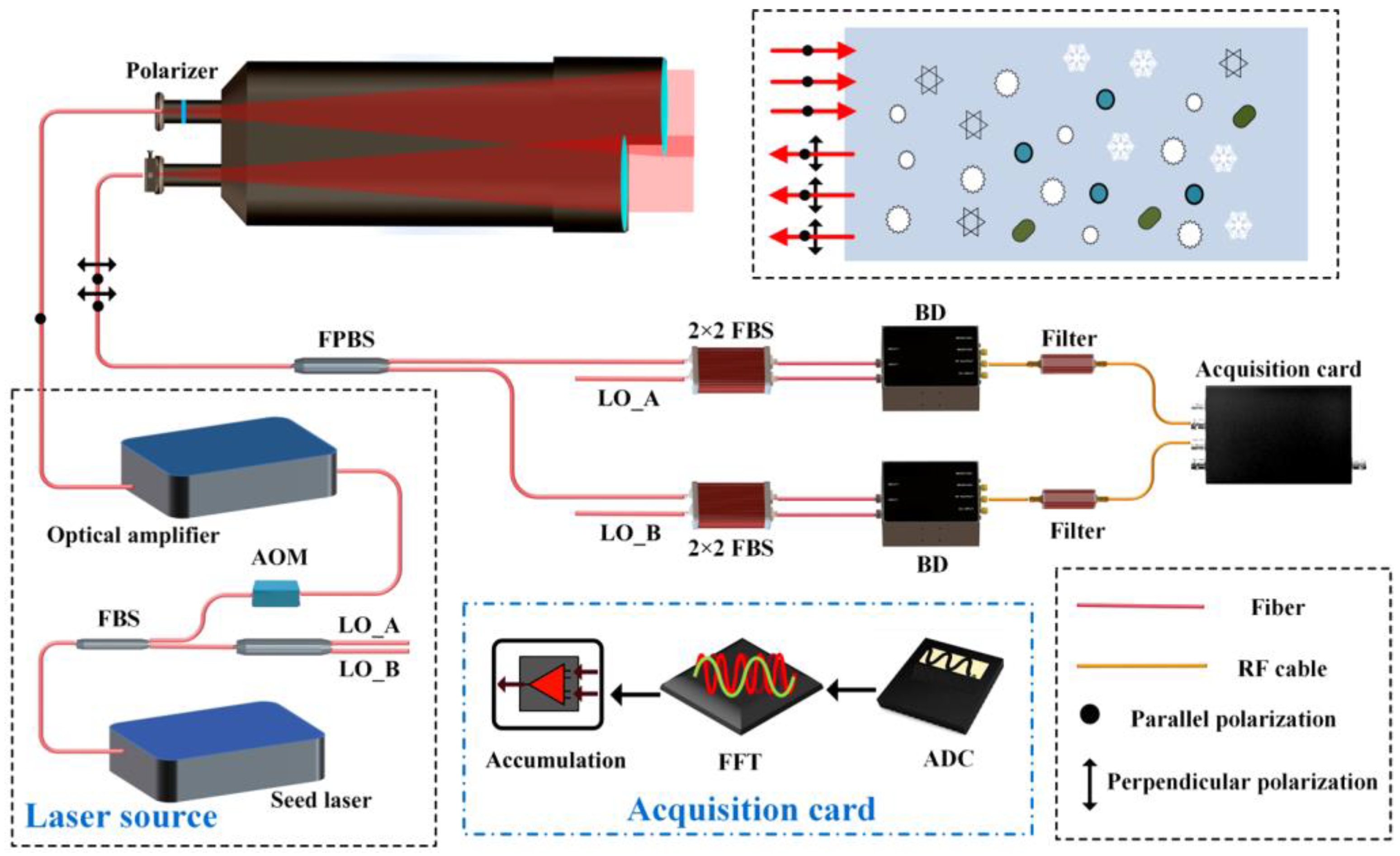
An all-fiber dual-channel polarization lidar using the coherent technique was established to measure the depolarization ratio of atmospheric aerosols at 1550 nm, as shown in Figure 1. The DPCDL system mainly consisted of a transmitter, a receiver, and a signal processor. The transmitter contained a laser source with the structure of a master-oscillator power amplifier (MOPA), a polarizer, and an aspherical paraxial telescope. The seed laser separated a portion of the continuous-wave lasers as the local oscillator, and the remaining portion was modulated by the AOM before amplification. The shift frequency of the AOM was 80 MHz. The laser source exports a 300 µJ, 800 ns pulse with a repetition rate of 10 kHz. The thermal effect of the optical fibers in the MOPA module induced changes in the polarization state of the beam. Hence, a polarizer with the extinction ratio of 35 dB was mounted to the emitting channel of the telescope. Finally, the pulsed laser beam was directionally transmitted into the atmosphere after being collimated by a collimating mirror in the telescope.
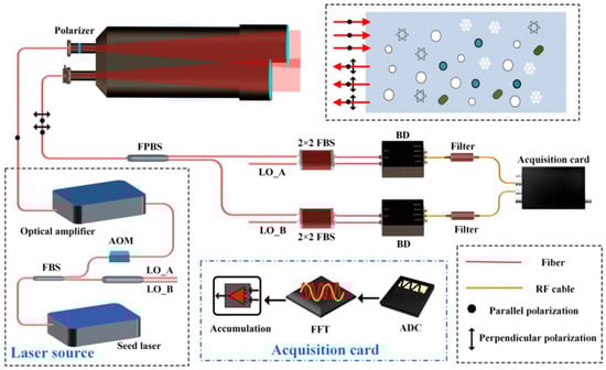
Figure 1.
Optical layout of the all-fiber dual-polarization coherent Doppler lidar. RF cable, radio-frequency cable; AOM, acousto-optic modulator; LO, local oscillator; FBS, fiber beam splitter; FPBS, fiber polarization beam splitter; BD, balanced detector; ADC, analog–digital converter; FFT, fast Fourier transform; FPGA, field-programmable gate array.
A paraxial telescope containing an aspherical lens with an aperture of 80 mm was used [27]. The paraxial telescope in the DPCDL was designed to isolate the emission and reception of the light beams and to facilitate the deployment of the polarizer in the laser transmission channel. To improve the reception efficiency of the backscattered signal and to minimize the blind range in the near field, the telescope was designed with a double-D shape, and the emitting telescope was mounted in front of the receiving telescope.
The performance of the receiving module depended on the extinction ratio of the fiber polarization splitter (FPBS), which was usually greater than 20 dB. This ensured an error of approximately 1% for the FPBS. The separated backscattered light of the two polarization states was coupled to the slow axis of the polarization-maintaining fiber and, finally, was connected through the FC/APC interface to ensure the matching of the polarization state of the local oscillator and signal light [28]. Moreover, a fiber polarizer was mounted to ensure that the polarization state of the local oscillator was close to the linear polarization state. Finally, the two mixed signals are individually coupled into the signal processor through polarization-maintaining fiber couplers.
The signal processor consisted of two balanced detectors, two bandpass filters, and an acquisition card. Moreover, balanced detectors and the bandpass filters were selected so that the same types were in each channel. The balanced detectors converted the mixed optical signals with the two polarizations into electrical signals and amplified them. A passive bandpass filter was selected to suppress high-frequency and low-frequency noise while completely passing through the Mie spectrum signal. Digital quantization of the analog signal was achieved with an analog–digital converter with a sampling rate of 250 MHz; the FFT and accumulation of the data were completed with a field-programmable gate array (FPGA). For each lidar pulse, the pulse spectral density (PSD) of the lidar signal was calculated in real time by the FPGA, and the PSDs were then averaged over 16,000 pulses. The system had a time resolution of 2.4 s and a distance resolution of 120 m. The key specifications of the DPCDL are listed in Table 1.

Table 1.
The main specifications of the DPCDL.
3. Experiments and Measurements
3.1. Experiments
3.1.1. Calibration of the Depolarization Ratio
Due to the differences in gain and responsiveness of the balance detectors used in the dual-polarization channels, the depolarization ratio measured with the DPCDL needed to be calibrated. A calibration procedure was designed such that a polarization-maintaining fiber splitter was used to replace the FPBS and split the backscattered signal evenly, which ensured that the signals of the dual-polarization channel were consistent. This design ensured the consistency of the signals of the dual-polarization channel and allowed for continuous long-term acquisition. The polarization states of the two output channels of the fiber splitter remained consistent. The highest extinction ratio of the fiber splitter was 22 dB. The beam-splitting ratio of the beam splitter was verified to be below 1.5%, which was acceptable. A three-hour experiment was conducted. The SNR served as the quality control criterion for the experimental data. For a coherent lidar system, the SNR is expressed as [25]
where is the coherent quantum efficiency, is the Planck constant, and and are the frequency of light and the bandwidth of the detector. The 19 dB SNR of the parallel-polarized signal was used for the quality control of the signal. This ensured the effectiveness of the dual-channel signals. So, the experimental data with SNRs higher than 19 dB were averaged, and the mean value was set as the calibration factor. Figure 2 shows the calibration factor over time, with its mean value of 1.13 and standard deviation of 0.017. The calibration factor mainly fluctuated in the small range of 1.05 to 1.17.
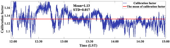
Figure 2.
Channel calibration data with a mean of 1.13 and a standard deviation of 0.017.
3.1.2. Evaluation of the Performance Evaluation of the DPCDL
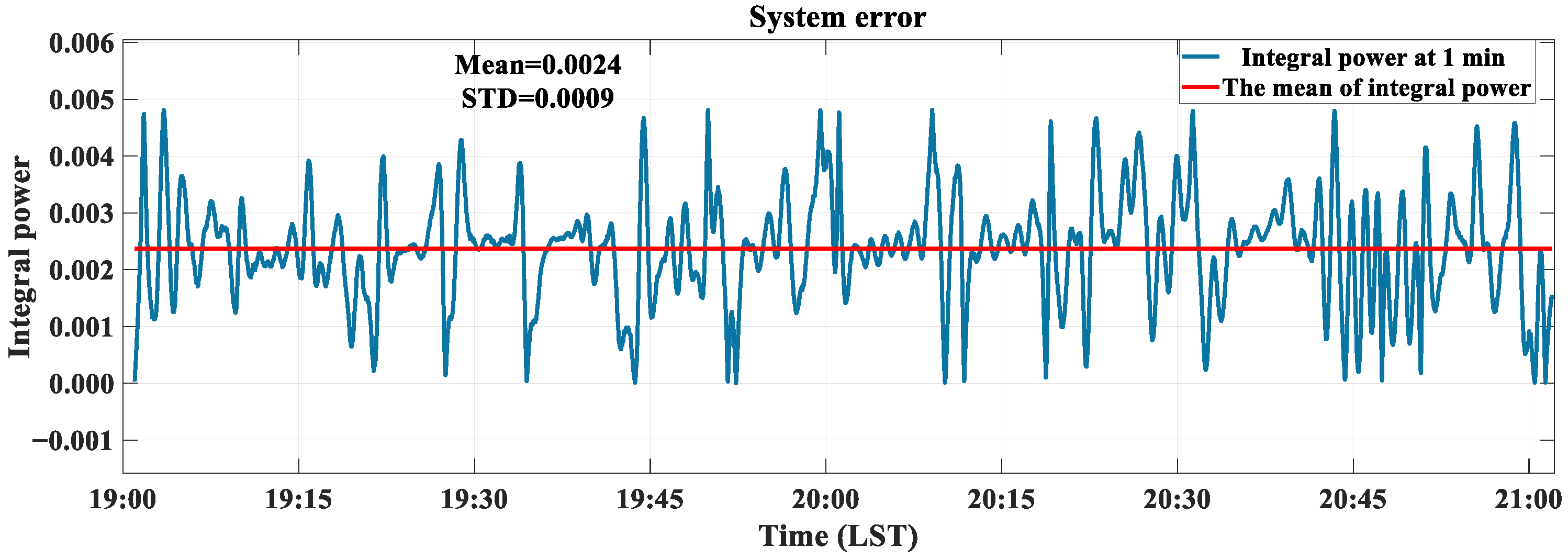
The DPCDL system utilized a laser source with an extinction ratio of 35 dB; theoretically, the error in the depolarization ratio measured with the DPCDL was lower than 0.001. However, the polarization state of the laser may change in many ways in an actual lidar. During the laser generation process, the polarization characteristics of lasers are related to the temperature of the optical resonance cavity [29]. The polarization state of the light transmitted along a fiber can change due to external stress, and it may also rotate when a fiber is in a curved state [30]. Moreover, when mode coupling occurs, there is an evolution of the polarization state in birefringent single-mode fibers [31]. The metal coating of a telescope’s surface typically changes the polarization of a backscattered signal, which seriously affects the measurement of the depolarization ratio of an aerosol [32]. Therefore, an evaluation of the systematic error is necessary. The mean value and the standard deviation (STD) were used as the evaluation criteria for the assessment of the DPCDL. Moreover, the random error during the observations was calculated. The Allan deviation was introduced to evaluate the impact of the accumulation time on the measured error. In addition, a formula was used to predict the modeled random error [33], which was compared with the random error in the observations.
In the DPCDL, the systematic error was related to the ability of the polarizer to control the direction of light vibration, the polarization splitting ability of the FPBS, differences in the dual-polarization channels, the noise of the acquisition card, etc. So, the uncertainty of a polarization lidar is also related to such aspects. The total systematic error is best estimated by estimating the error space of the complete system, so an experiment was conducted to measure it. Based on the DPCDL system, a low-energy pulse from the seed module was emitted from one telescope with a polarizer and directly received by another telescope before being coupled into the receiver of the DPCDL. This experiment considered the changes in the polarization state of a beam during transmission in the DPCDL without the atmospheric scattering effect. So, the experimental data represented the systematic error. Figure 3 shows that the mean value and STD of the systematic error were 0.0024 and 0.0009 with a 1-min averaging window. Finally, the DPCDL performed well and was capable of achieving high-precision measurement of the depolarization ratios of aerosols.
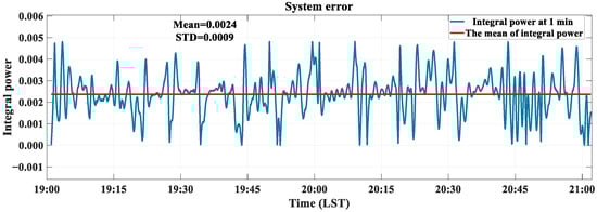
Figure 3.
Systematic error of the DPCDL: systematic error with a mean value of 0.0024 and a standard deviation of 0.0009. There was a fluctuation below 0.0048 with a 1 min averaging window.
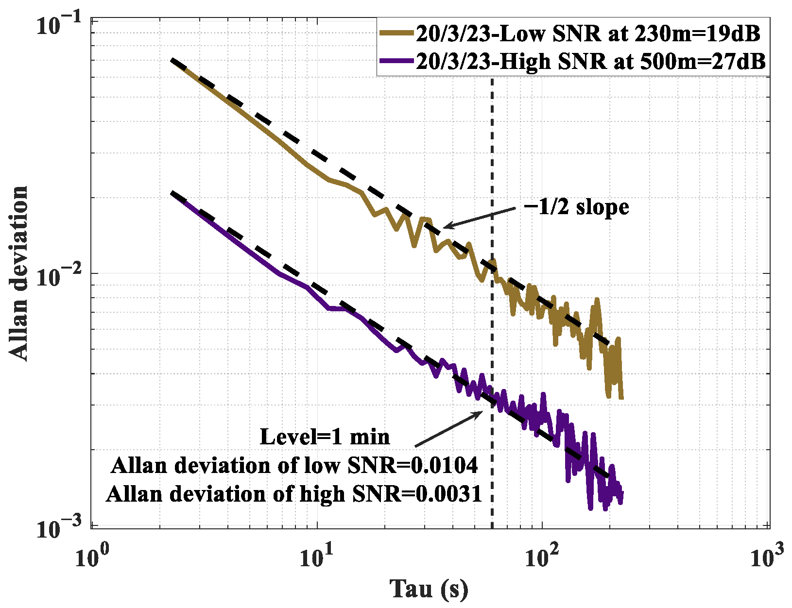
In addition to the systematic error, the random error was estimated. The measurement error was related to the integration time of cumulative smoothing and the SNR of the signals. The integration time is an important parameter in the cumulative smoothing method. The Allan deviation was used to evaluate the impact of the integration time on the random error. An experiment conducted on March 20th, 2023, was used as a measurement case. Due to the precipitation beforehand, the aerosol load in the atmosphere was low. Hence, the aerosol depolarization ratios were small. Therefore, these conditions could be used to evaluate the random error of the DPCDL. The Allan deviation is also related to the SNR, so signals with a low SNR of 19 dB and a high SNR of 27 dB were selected. A time plot of the measured integral power of the noise spectrum at the low SNR and high SNR with an averaging window of 1 min can be found in Appendix A. Figure 4 shows the Allan deviations with the low SNR and high SNR. The slopes of the Allan deviation on a logarithmic scale were close to −1/2. It was illustrated that the random error with an integration time of 1 min was larger than the systematic error with a 1-min averaging window. To ensure the accuracy of the depolarization ratio, the SNR threshold used for quality control was set to 19 dB. The Allan deviation with the low SNR of 19 dB was significantly larger than that with the high SNR of 27 dB. During the data processing, the cumulative smoothing window is generally set to 1 min. Moreover, when the integration time was 1 min, the Allan deviation at the low SNR was 0.0104 and the Allan deviation at the high SNR was 0.0031. As the integration time increased or the SNR increased, the Allan deviation gradually decreased.
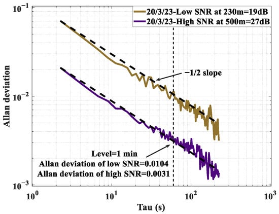
Figure 4.
Allan deviation of the measurements that were recorded with a low SNR of 19 dB and a high SNR of 27 dB on the 20th of March. The Allan deviation gradually decreased with the increase in the integration time, and the Allan deviation with the low SNR was higher than that with the high SNR. The Allan deviations with a 1 min averaging window at the low SNR and the high SNR were 0.0104 and 0.0031, respectively.
To evaluate the impact of the SNR on the measurements, the relative random error (RRE) was introduced. To describe a random variable , the RRE is expressed as [33]
where is a random variable, and and are the standard deviation and the mean value of , respectively. The errors of the dual-polarization half-width integrals from Equation (3) were within the random error budget. However, the calibration factor of the depolarization ratio was regarded as a constant. The random error can be approximatively expressed as [33]
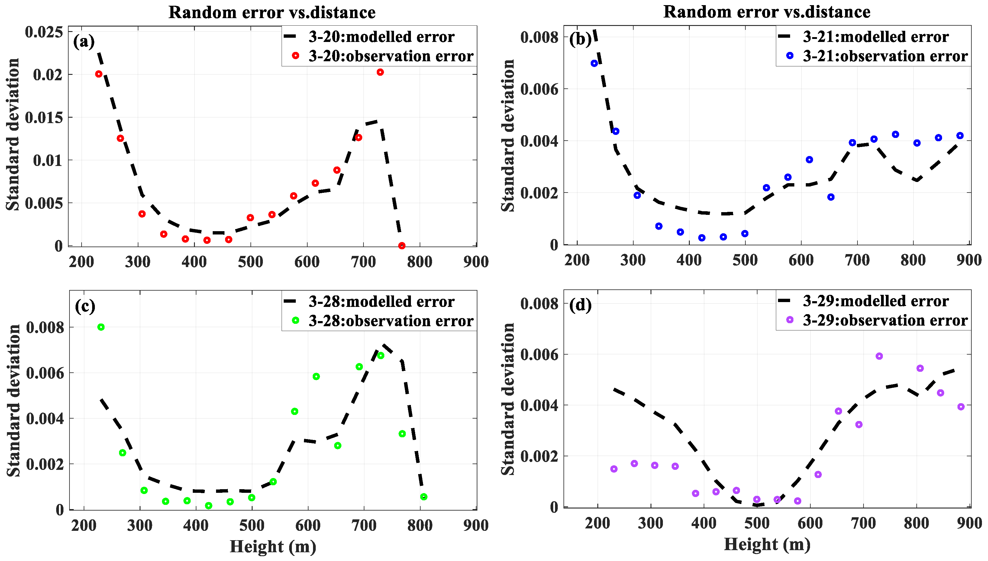
where is the number of laser pulses. The laser frequency was 10 kHz. Figure 5a–d show the modeled random errors for the 20th, 21st, 28th, and 29th of March. They were compared with the random errors in the observations, which were consistent. The random errors in the observations were proven to be reasonable and accurate. The random errors were mainly distributed below 0.03, and they were below 0.01 at high SNRs. The DOCDL was able to achieve high-precision observation of the aerosol depolarization ratio.
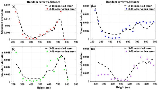
Figure 5.
The modeled random error and the random error of observations on (a) March 20, (b) March 21, (c) March 28, and (d) March 29.
3.2. Comparison of Continuous Observations in Two Measurement Cases
To demonstrate the performance of the DPCDL, a comparison of a co-located DPCDL and micro-pulse lidar with a wavelength of 532 nm was conducted. It was reported that different detection wavelengths induce different depolarization spectra [34]. The DPCDL and MPL had different sensitivities; thus, their depolarization ratios were different. It should be emphasized that the depolarization ratios measured with the DPCDL and MPL exhibited high consistency, which verified the authenticity of the DPCDL’s measurements.
The direct power detection method for the dual-polarization components was adopted for the MPL. Spatial optical devices and single-photon detectors were used. The laser source emitted a 500 µJ, 13 ns pulse with a repetition rate of 4 kHz at a wavelength of 532 nm. The temporal and spatial resolutions of the MPL were 15 min and 15 m, respectively. To calibrate the depolarization ratio of the MPL, the concept of “∆90°-calibration” was applied; then, the depolarization ratio was calculated [35,36]. Two sets with a half-wave plate at angles of (0°, 45°) and (22.5°, −22.5°) were used for the calibration, which was confirmed to be effective in atmospheric science experiments.
Two comparative experiments were conducted at the Ocean University of China (36.15°N, 120.51°E). The vertical distributions of the depolarization ratios were simultaneously detected with the co-located instruments, namely, the DPCDL and the MPL.
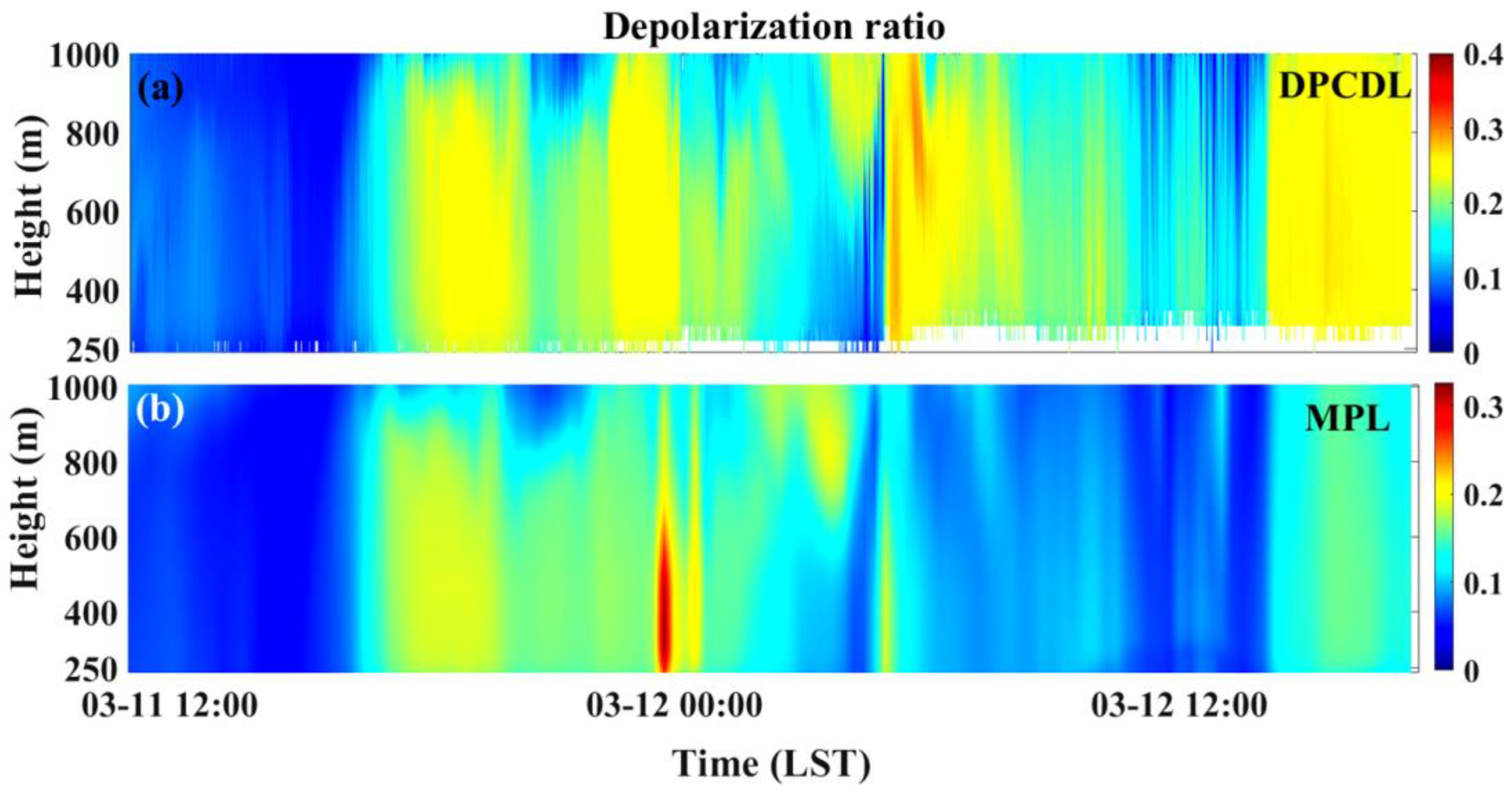
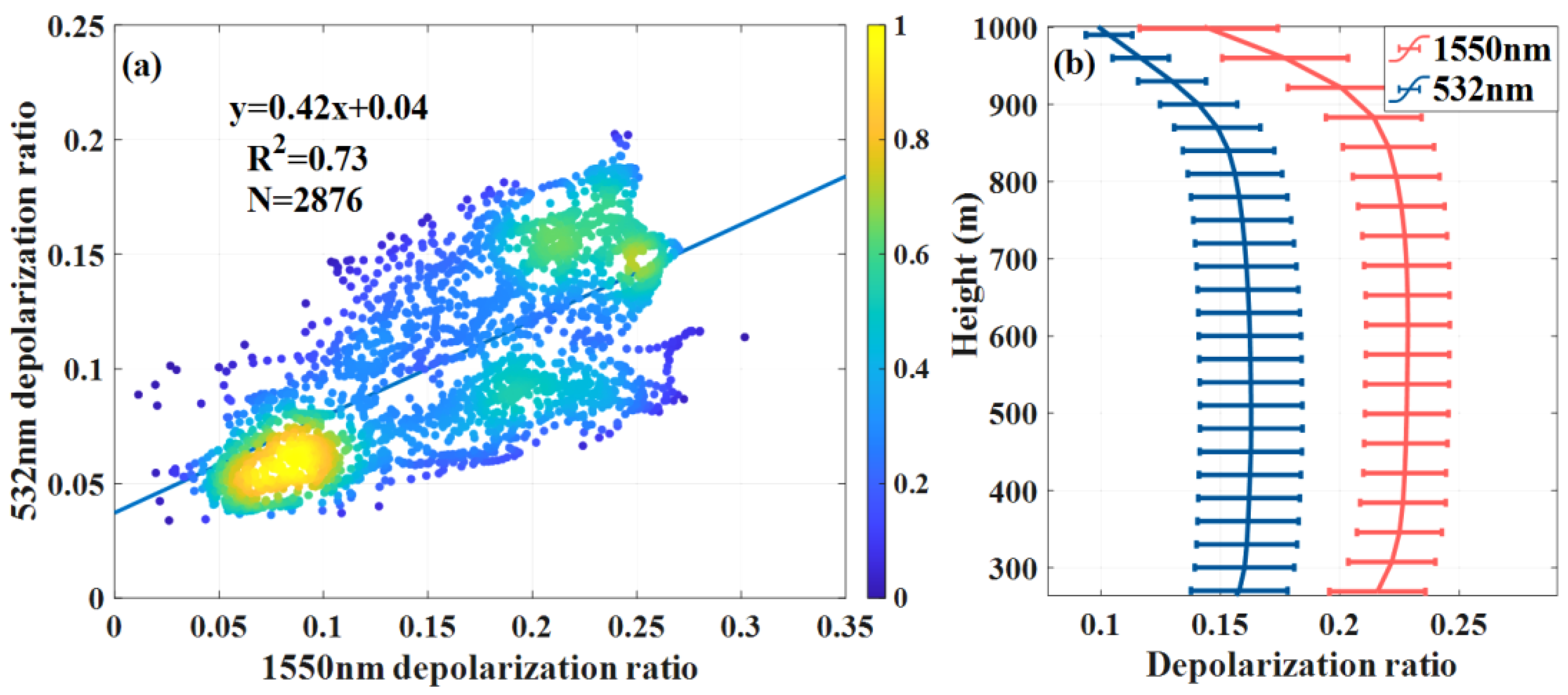
The first experimental results for the observations of atmospheric aerosol are shown in Figure 6 and Figure 7. The vertical depolarization ratios measured with the DPCDL are presented in Figure 6a with a temporal resolution of 2.4 s and a spatial resolution of 120 m. The vertical depolarization ratios observed with the MPL are shown in Figure 6b with a temporal resolution of 15 min and a spatial resolution of 15 m. The high values of the depolarization ratio between 16:00 LST and 18:00 LST on the 11th of March indicate the presence of non-spherical aerosols in the atmosphere, which may have been caused by severe air pollution. The atmosphere may have contained a small amount of dust. On the contrary, the low values of the depolarization ratio revealed the lack of non-spherical particles in the atmosphere. Aerosols with low depolarization ratios are mainly water-soluble. It can be seen in these two figures that the depolarization ratios of aerosols containing dust were significantly higher than those of water-soluble aerosols. Figure 7a shows a scatter diagram of the depolarization ratios at 1550 nm and 532 nm with a statistical size of 2876. One can see that the depolarization ratio values from the DPCDL were mostly below 0.3 during the observation period, while the depolarization ratio values from the MPL were mostly below 0.2. It is shown that the results from the DPCDL and MPL agreed well, with a correlation coefficient of 0.73 and a slope of 0.42. Figure 7b presents the average depolarization ratio profiles from the DPCDL and MPL between 16:00 LST and 18:00 LST on the 11th of March, 2023. The first-observation line plots of the depolarization ratios measured with the DPCDL and MPL at 400 m, 600 m, and 800 m can be found in Appendix B. It was found that the depolarization ratios from the DPCDL and MPL had consistent tendencies.

Figure 6.
The first 31-h observations with the co-located DPCDL and MPL: (a) The time series of the depolarization ratios from the DPCDL with a time resolution of 2.4 s. (b) The time series of the depolarization ratios from the MPL with a time resolution of 15 min.

Figure 7.
The first 31-h observations with the co-located DPCDL and MPL: (a) A scatter diagram of the depolarization ratio measurements of the DPCDL and MPL with a correlation coefficient of 0.73 and a slope of 0.42. (b) The depolarization ratio profile from the DPCDL and MPL. The data from the period of 16:00 to 18:00 on the 11th of March are used.
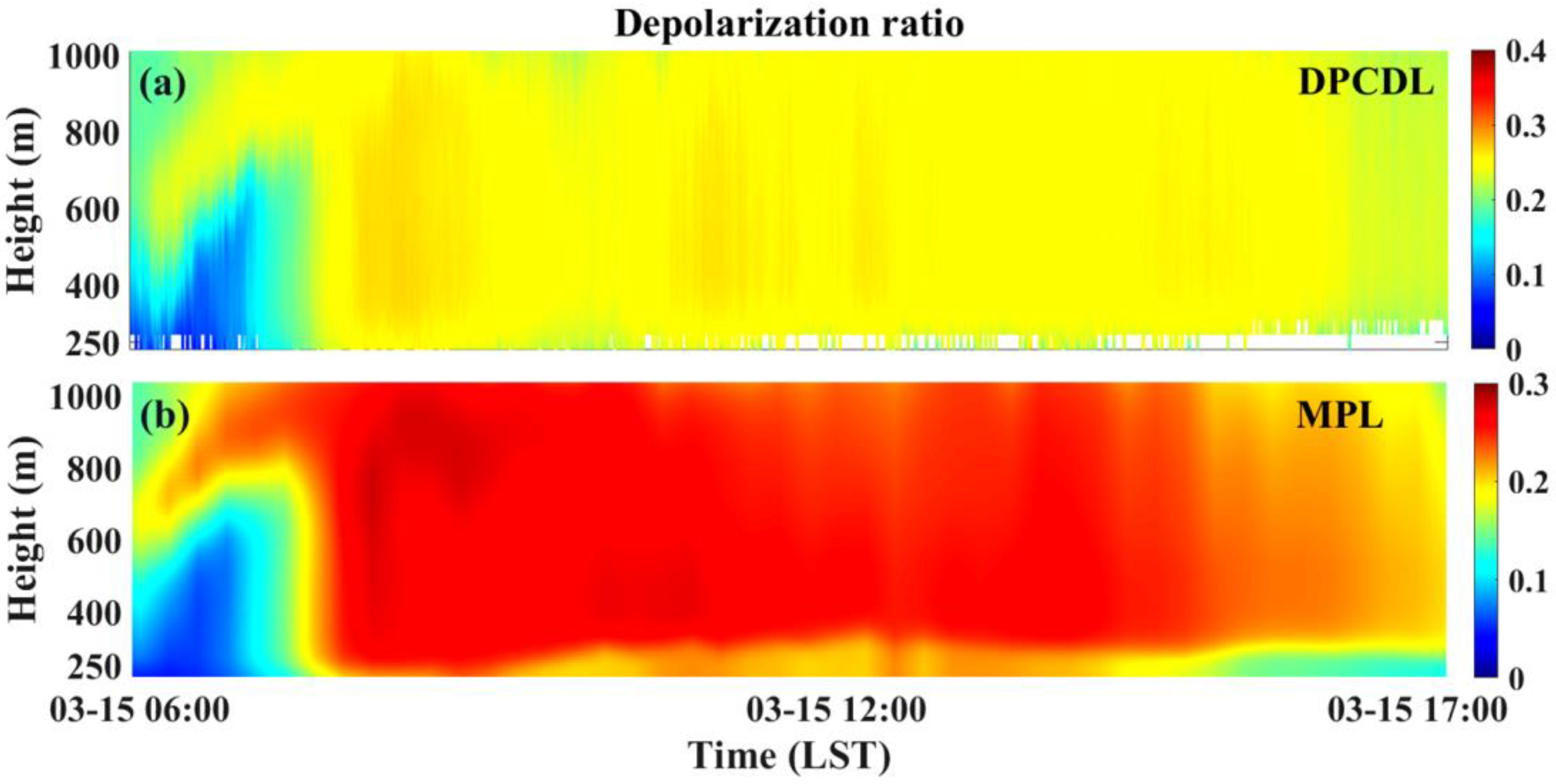
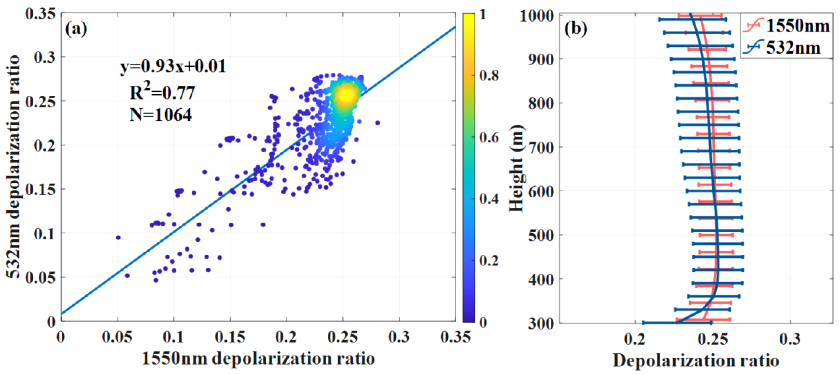
The results of the second experimental observation of dust layers are shown in Figure 8 and Figure 9. The vertical distributions of the depolarization ratios observed with the DPCDL and MPL are shown in Figure 8a and Figure 8b, respectively. The results from the two systems were consistent. Figure 9a shows a scatter diagram with a statistical size of 1064. It was shown that the depolarization ratios from the DPCDL and MPL agreed well, with a correlation coefficient of 0.77 and a slope of 0.93. Figure 9b presents the mean values of the depolarization ratio profiles observed with the DPCDL and MPL between 06:15 LST and 17:00 LST on the 15th of March, 2023. The line plots of the second observation of depolarization ratios with the DPCDL and MPL at 400 m, 600 m, and 800 m can be found in Appendix B. The tendencies of the depolarization ratios in these two systems were consistent.
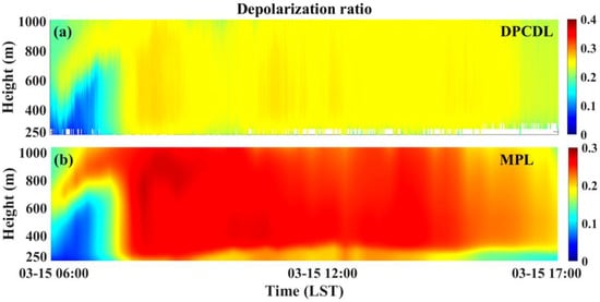
Figure 8.
The second 11-h observations with the co-located DPCDL and MPL: (a) The time series of the depolarization ratios measured with the DPCDL. (b) The time series of the depolarization ratios measured with the MPL.
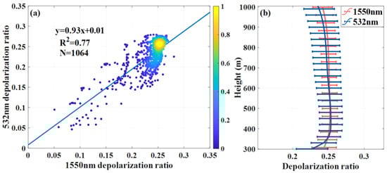
Figure 9.
The second 11-h observations with the co-located DPCDL and MPL: (a) A scatter diagram of the depolarization ratio measurements with the DPCDL and MPL, with a correlation coefficient of 0.77 and a slope of 0.93. (b) The depolarization ratio profiles from the DPCDL and MPL. The data from the period of 06:15 to 17:00 on the 15th of March are used.
The meteorological conditions during the two observations were different. The observation results from the two co-located systems showed dual-wavelength depolarization ratios of aerosols with small and large particle sizes. It was obvious that the depolarization ratio for the large particle size in the second observation experiment was significantly higher than that for the small particle size in the first observation experiment. The results in Figure 6a and Figure 8a are highly consistent to those of Wang [19]. The dual-wavelength depolarization ratios of aerosols with different particle sizes exhibited different patterns [21]. In the case of aerosols with a small particle size, the depolarization ratio values at 1550 nm were higher than those at 532 nm. In the case of aerosols with a large particle size, the depolarization ratios at 1550 nm and 532 nm were roughly equal. The patterns could provide us with more information on classifying aerosol types.
4. Discussion
The DPCDL is a polarization lidar system based on the coherence technique. The paraxial telescope design in the DPCDL greatly eliminates the interference of light undergoing specular reflection, which ensures the stability of the system. The all-fiber structure of the DPCDL is convenient for its miniaturization and integration, and it ensures its stability in the event of external environmental changes. Furthermore, the DPCDL utilizes two balanced detectors for photoelectric conversion, which allows it to avoid the problem of high cost found in traditional 1550 nm MPLs based on high-performance single-photon detectors. Finally, the DPCDL has the potential to achieve the simultaneous observation of wind speed and the aerosol depolarization ratio; as a result, the depolarization ratio and wind speed data that are obtained can be used to analyze the sources of non-spherical pollutant particles and predict their diffusion paths. This work will be carried out in the future.
1550 nm lidars can ensure the safety of the human eye and have strong penetration, making them widely used in the field of aerosol detection. More and more research is being conducted on polarization lidars working at 1550 nm. The depolarization ratio at 1550 nm is an important parameter that reflects the shape of aerosols, and it is commonly used in research on aerosol classification and aerosol–cloud interactions. This research on the 1550 nm DPCDL is of great significance.
However, since a linearly polarized light source is applied, the SNR of the perpendicular-polarization channel is usually low, which limits the observation accuracy and observation distance. Compared with linearly polarized laser sources, a circularly polarized light may have more obvious advantages, and more work is required to demonstrate this. The use of circularly polarized light sources will be implemented in subsequent work.
5. Conclusions
To obtain the depolarization ratio at a wavelength of 1550 nm, an all-fiber dual-polarization coherent Doppler lidar with a wavelength of 1550 nm was designed in this study. The stability of the system was proven in performance evaluation experiments. The system successfully achieved the measurement of the depolarization ratio at 1550 nm. The depolarization ratios of aerosols such as haze and dust were detected, and the results were in line with expectations. Furthermore, two continuous observation campaigns involving different aerosols, including a clean continental atmosphere, haze, and dust, were performed. When observing aerosols with different particle sizes, the depolarization ratios at two wavelengths exhibited different relationships. These relationships provide a foundation for further work on the classification of aerosols.
Based on the coherent detection technique, the depolarization ratios of atmospheric aerosols were measured at a wavelength of 1550 nm. The systematic error and random error were estimated for use in a performance evaluation, and the results showed that the performance was good. Compared to a single-channel polarized coherent Doppler lidar, the DPCDL has the potential to synchronously observe the atmospheric wind speed and depolarization ratio. The double-channel design helps to increase the SNR of the wind speed signal and the detection range, allowing it to better adapt to weather changes. The atmospheric polarization information that was obtained can help in more accurately inverting the characteristics of atmospheric aerosols, such as their extinction coefficient and backscatter coefficient. The DPCDL has the advantages of a high stability, the possibility of measurement in the day and night, and a low price. Finally, the DPCDL can be employed in conjunction with other devices to measure optical parameters, such as the color ratio. Above all, the DPCDL has great application prospects in the field of atmospheric detection.
Author Contributions
R.Y.: conceptualization, methodology, validation, investigation, writing—original draft; Q.W.: conceptualization, supervision, writing—review and editing; G.D.: conceptualization, funding, writing—review and editing; X.C.: formal analysis; C.R.: funding; J.L.: writing—review and editing; D.L.: writing—review; X.W.: conceptualization; H.C.: conceptualization; S.Q.: writing—review and editing; S.W.: writing—review. All authors have read and agreed to the published version of the manuscript.
Funding
This study was jointly supported by the Laoshan Laboratory Science and Technology Innovation Projects under grant LSKJ202201202 and the National Natural Science Foundation of China (NSFC) under grants 61975191, 41905022, and U2106210.
Data Availability Statement
Due to confidentiality agreements, the supporting data can only be made available to bona fide researchers subject to a non-disclosure agreement. To access the data, please contact wangqichao@ouc.edu.cn at Ocean University of China.
Acknowledgments
We thank our colleagues for their kind support for this work.
Conflicts of Interest
The authors declare no conflict of interest.
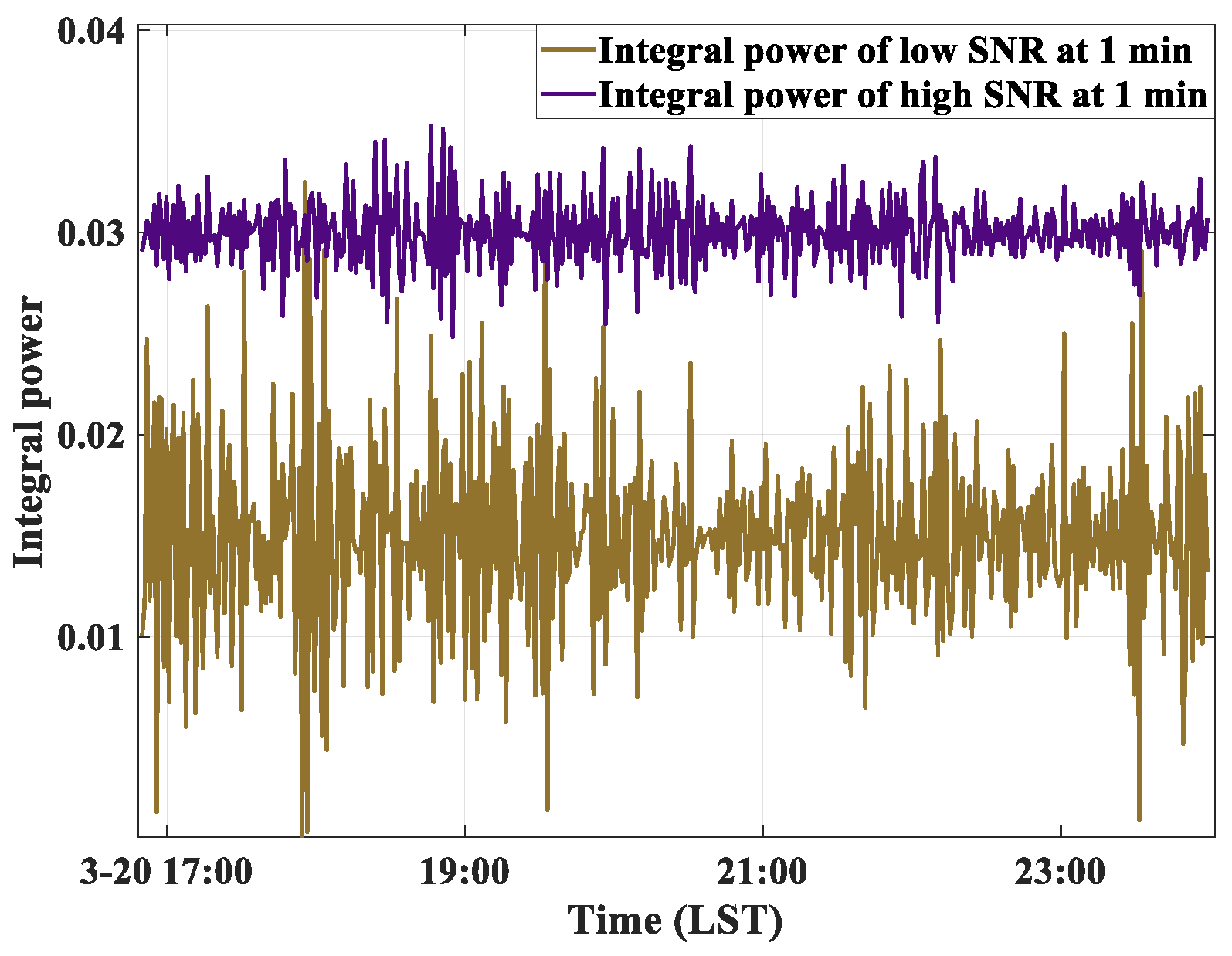
Appendix A
Figure A1 shows a time plot of measured integral power of the noise spectrum at a low SNR and a high SNR with an averaging window of 1 min. It was found that the fluctuation of the integral power of the noise spectrum with a low SNR was higher than that with a high SNR.
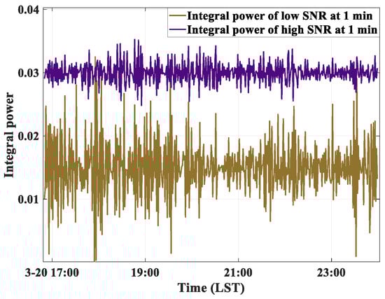
Figure A1.
Time plot of the DPCDL’s integral power of the noise spectrum with a 1 min averaging window.
Figure A1.
Time plot of the DPCDL’s integral power of the noise spectrum with a 1 min averaging window.
Appendix B
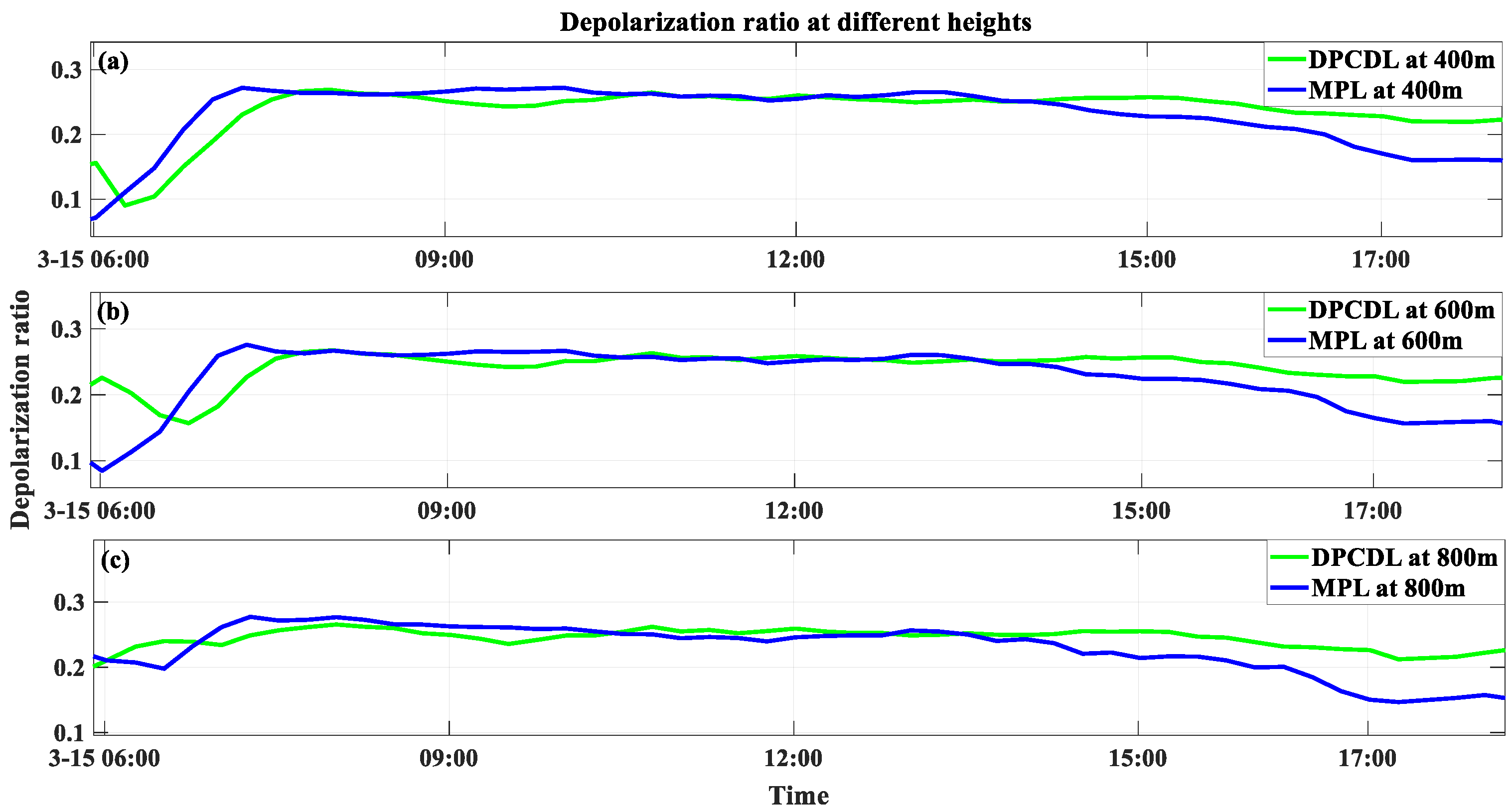
Figure A2 shows the first-observation line plots of the depolarization ratios obtained with the DPCDL and MPL at 400 m, 600 m, and 800 m. Figure A3 shows the second-observation line plots of the depolarization ratios obtained with the DPCDL and MPL at 400 m, 600 m, and 800 m. The depolarization ratios obtained with the DPCDL and MPL demonstrated consistency.
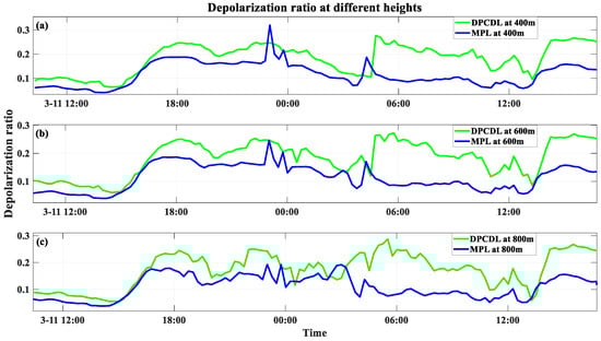
Figure A2.
The first-observation line plots of the depolarization ratios obtained with the DPCDL and MPL at 400 m, 600 m, and 800 m: (a) The line plot at 400 m. (b) The line plot at 600 m. (c) The line plot at 800 m.
Figure A2.
The first-observation line plots of the depolarization ratios obtained with the DPCDL and MPL at 400 m, 600 m, and 800 m: (a) The line plot at 400 m. (b) The line plot at 600 m. (c) The line plot at 800 m.
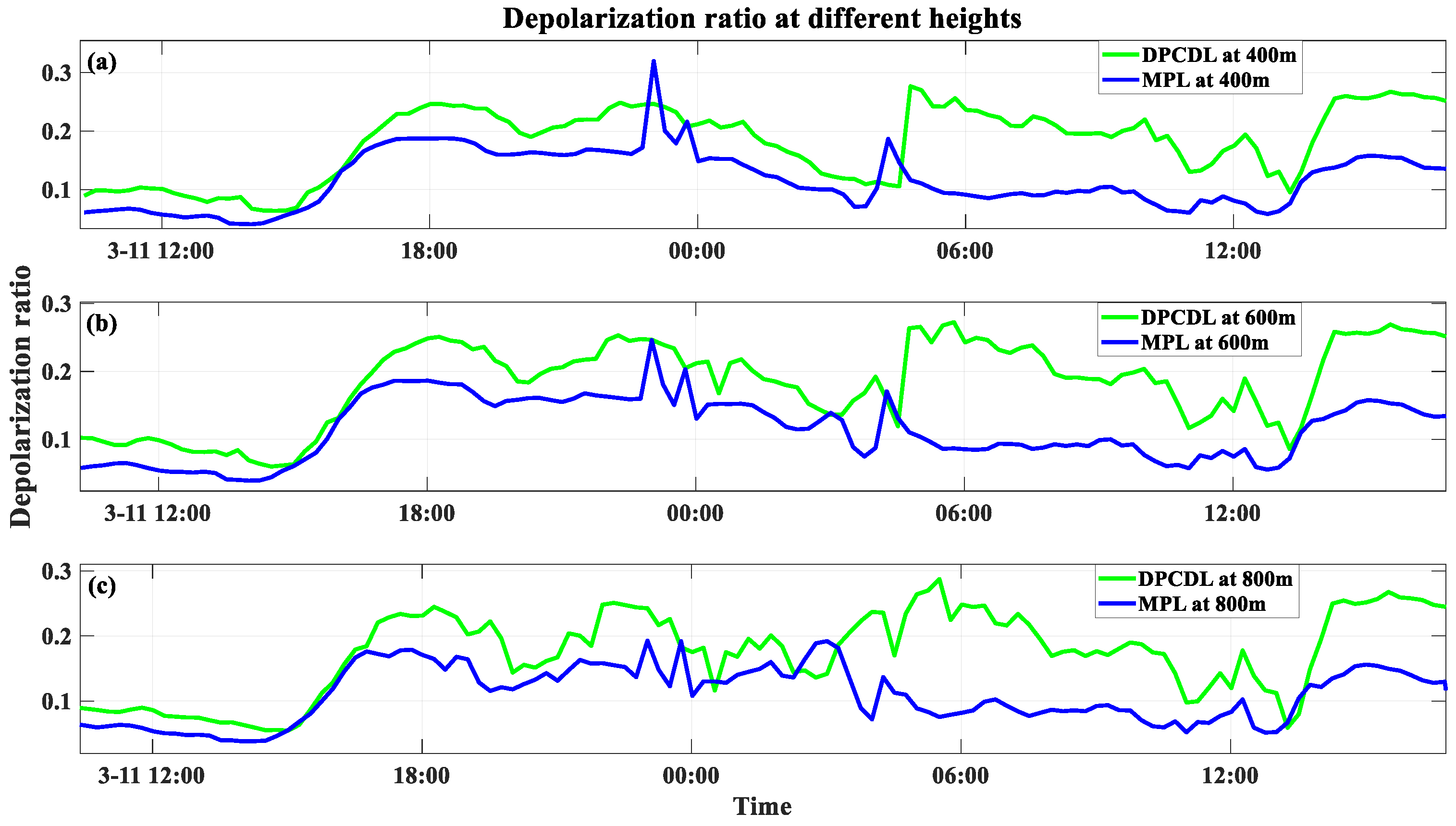
Figure A3.
The second-observation line plots of the depolarization ratios obtained with the DPCDL and MPL at 400 m, 600 m, and 800 m: (a) The line plot at 400 m. (b) The line plot at 600 m. (c) The line plot at 800 m.
Figure A3.
The second-observation line plots of the depolarization ratios obtained with the DPCDL and MPL at 400 m, 600 m, and 800 m: (a) The line plot at 400 m. (b) The line plot at 600 m. (c) The line plot at 800 m.
References
- Li, X.; Zhang, P.; Gao, L.; Zhang, X. Global Change of Aerosol Optical Depth Based on Satellite Remote Sensing Data. Sci. Technol. Rev. 2015, 33, 30–39. [Google Scholar]
- Haywood, J.; Boucher, O. Estimates of the Direct and Indirect Radiative Forcing Due to Tropospheric Aerosols: A Review. Rev. Geophys. 2000, 38, 513–543. [Google Scholar] [CrossRef]
- Sokolik, I.N.; Toon, O.B. Direct Radiative Forcing by Anthropogenic Airborne Mineral Aerosols. Nature 1996, 381, 681–683. [Google Scholar] [CrossRef]
- Asaka, K.; Yanagisawa, T.; Hirano, Y. 1.5 μm Eye-Safe Coherent Lidar System for Wind Velocity Measurement. In Proceedings of the Lidar Remote Sensing for Industry and Environment Monitoring, Sendai, Japan, 9–12 October 2000; Singh, U.N., Asai, K., Ogawa, T., Singh, U.N., Itabe, T., Sugimoto, N., Eds.; SPIE: Bellingham, DC, USA, 2001; Volume 4153, pp. 321–328. [Google Scholar] [CrossRef]
- Xia, H.; Shentu, G.; Shangguan, M.; Xia, X.; Jia, X.; Wang, C.; Zhang, J.; Pelc, J.S.; Fejer, M.M.; Zhang, Q.; et al. Long-Range Micro-Pulse Aerosol Lidar at 1.5 μm with an Upconversion Single-Photon Detector. Opt. Lett. 2015, 40, 1579–1582. [Google Scholar] [CrossRef] [PubMed]
- Shangguan, M.; Xia, H.; Dou, X.; Qiu, J.; Yu, C. Development of Multifunction Micro-Pulse Lidar at 1.5 Micrometer. EPJ Web Conf. 2020, 237, 07010. [Google Scholar] [CrossRef]
- Shang, X.; Xia, H.; Dou, X.; Shangguan, M.; Li, M.; Wang, C. Adaptive Inversion Algorithm for 1.5 μm Visibility Lidar Incorporating in Situ Angstrom Wavelength Exponent. Opt. Commun. 2018, 418, 129–134. [Google Scholar] [CrossRef]
- Jain, D.; Mehra, R. Performance Analysis of Free Space Optical Communication System for S, C and L Band. In Proceedings of the 2017 International Conference on Computer, Communications and Electronics (Comptelix), Jaipur, India, 1–2 July 2017; pp. 183–189. [Google Scholar] [CrossRef]
- Schotland, R.M.; Sassen, K.; Stone, R. Observations by Lidar of Linear Depolarization Ratios for Hydrometeors. J. Appl. Meteorol. Climatol. 1971, 10, 1011–1017. [Google Scholar] [CrossRef]
- Liu, D.; Qi, F.; Jin, C.; Yue, G.; Zhou, J. Lidar Detection of Depolarization Ratio of Cirrus Cloud and Dust Aerosol over Hefei. Atmos. Sci. 2003, 27, 1093–1100. [Google Scholar]
- Luü, L.; Liu, W.; Zhang, T.; Lu, Y.; Qi, S. A New Micro-Pulse Lidar for Atmospheric Horizontal Visibility Measurement. Chin. J. Lasers 2014, 41, 908005. [Google Scholar] [CrossRef]
- Zhu, C.; Cao, N.; Yang, F.; Yang, S.; Xie, Y. Micro Pulse Lidar Observations of Aerosols in Nanjing. Laser Optoelectron. Prog. 2015, 52, 050101. [Google Scholar]
- Wang, W.; Yi, F.; Liu, F.; Zhang, Y.; Yin, Z. Characteristics and Seasonal Variations of Cirrus Clouds from Polarization Lidar Observations at a 30° N Plain Site. Remote Sens. 2020, 12, 3998. [Google Scholar] [CrossRef]
- Tomoaki, N.; Nobuo, S.; Ichiro, M.; Atsushi, S.; Boyan, T.; Hajime, O. Algorithm to Retrieve Aerosol Optical Properties from High-Spectral-Resolution Lidar and Polarization Mie-Scattering Lidar Measurements. IEEE Trans. Geosci. Remote Sens. 2008, 46, 4094–4103. [Google Scholar] [CrossRef]
- Pal, S.R.; Carswell, A.I. Polarization Properties of Lidar Scattering from Clouds at 347 nm and 694 nm. Appl. Opt. 1978, 17, 2321–2328. [Google Scholar] [CrossRef]
- Sugimoto, N.; Lee, C.H. Characteristics of Dust Aerosols Inferred from Lidar Depolarization Measurements at Two Wavelengths. Appl. Opt. 2006, 45, 7468–7474. [Google Scholar] [CrossRef] [PubMed]
- Baars, H.; Seifert, P.; Engelmann, R.; Wandinger, U. Target Categorization of Aerosol and Clouds by Continuous Multiwavelength-Polarization Lidar Measurements. Atmos. Meas. Tech. 2017, 10, 3175–3201. [Google Scholar] [CrossRef]
- Qiu, J.; Xia, H.; Shangguan, M.; Dou, X.; Li, M.; Wang, C.; Shang, X.; Lin, S.; Liu, J. Micro-Pulse Polarization Lidar at 1.5 μm Using a Single Superconducting Nanowire Single Photon Detector. Opt. Lett. 2017, 42, 4454–4457. [Google Scholar] [CrossRef] [PubMed]
- Wang, C.; Xia, H.; Shangguan, M.; Wu, Y.; Wang, L.; Zhao, L.; Qiu, J.; Zhang, R. 1.5 μm Polarization Coherent Lidar Incorporating Time-Division Multiplexing. Opt. Express 2017, 25, 20663–20674. [Google Scholar] [CrossRef] [PubMed]
- Abari, C.F.; Chu, X.; Hardesty, R.M.; Mann, J. A Reconfigurable All-Fiber Polarization-Diversity Coherent Doppler Lidar: Principles and Numerical Simulations. Appl. Opt. 2015, 54, 8999–9009. [Google Scholar] [CrossRef]
- Vakkari, V.; Baars, H.; Bohlmann, S.; Bühl, J.; Komppula, M.; Mamouri, R.-E.; O’Connor, E.J. Aerosol Particle Depolarization Ratio at 1565 nm Measured with a Halo Doppler Lidar. Atmos. Chem. Phys. 2021, 21, 5807–5820. [Google Scholar] [CrossRef]
- Xu, Z.; Zhang, H.; Chen, K.; Pan, S. Compact All-Fiber Polarization Coherent Lidar Based on a Polarization Modulator. IEEE Trans. Instrum. Meas. 2020, 69, 2193–2198. [Google Scholar] [CrossRef]
- Zhang, H.; Wu, S.; Wang, Q.; Liu, B.; Yin, B.; Zhai, X. Airport Low-Level Wind Shear Lidar Observation at Beijing Capital International Airport. Infrared Phys. Technol. 2019, 96, 113–122. [Google Scholar] [CrossRef]
- Huffaker, R.M.; Henderson, S.; Rees, D.; Gatt, P. Wind Lidar. In Laser Remote Sensing; CRC Press: Boca Raton, FL, USA, 2005. [Google Scholar] [CrossRef]
- Chouza, F.; Reitebuch, O.; Groß, S.; Rahm, S.; Freudenthaler, V.; Toledano, C.; Weinzierl, B. Retrieval of Aerosol Backscatter and Extinction from Airborne Coherent Doppler Wind Lidar Measurements. Atmos. Meas. Tech. 2015, 8, 2909–2926. [Google Scholar] [CrossRef]
- Sassen, K. The Polarization Lidar Technique for Cloud Research: A Review and Current Assessment. Bull. Am. Meteorol. Soc. 1991, 72, 1848–1866. [Google Scholar] [CrossRef]
- Ge, X.; Chen, S.; Zhang, Y.; Chen, H.; Guo, P.; Mu, T.; Yang, J. Telescope Design for 2 μm Spacebased Coherent Wind Lidar System. Opt. Commun. 2014, 315, 238–242. [Google Scholar] [CrossRef]
- Ma, T.; Tong, S.; Nan, H.; Jia, X. Effect of Polarization Property of Signal Light on Mixing Efficiency of Space Coherent Detection. Laser Optoelectron. Prog. 2017, 54, 020604. [Google Scholar] [CrossRef]
- Choquette, K.D.; Richie, D.A.; Leibenguth, R.E. Temperature Dependence of Gain-guided Vertical-cavity Surface Emitting Laser Polarization. Appl. Phys. Lett. 1994, 64, 2062–2064. [Google Scholar] [CrossRef]
- Ross, J.N. The Rotation of the Polarization in Low Birefringence Monomode Optical Fibres Due to Geometric Effects. Opt. Quantum Electron. 1984, 16, 455–461. [Google Scholar] [CrossRef]
- Monerie, M.; Jeunhomme, L. Polarization Mode Coupling in Long Single-Mode Fibres. Opt. Quantum Electron. 1980, 12, 449–461. [Google Scholar] [CrossRef]
- Di, H.; Hua, D.; Yan, L.; Hou, X.; Wei, X. Polarization Analysis and Corrections of Different Telescopes in Polarization Lidar. Appl. Opt. 2015, 54, 389–397. [Google Scholar] [CrossRef]
- Cezard, N.; Mehaute, S.L.; Gouët, J.L.; Valla, M.; Goular, D.; Fleury, D.; Planchat, C.; Dolfi-Bouteyre, A. Performance Assessment of a Coherent DIAL-Doppler Fiber Lidar at 1645 nm for Remote Sensing of Methane and Wind. Opt. Express 2020, 28, 22345–22357. [Google Scholar] [CrossRef]
- Haarig, M.; Ansmann, A.; Baars, H.; Jimenez, C.; Veselovskii, I.; Engelmann, R.; Althausen, D. Depolarization and Lidar Ratios at 355, 532, and 1064 Nm and Microphysical Properties of Aged Tropospheric and Stratospheric Canadian Wildfire Smoke. Atmos. Chem. Phys. 2018, 18, 11847–11861. [Google Scholar] [CrossRef]
- Dai, G.; Wu, S.; Song, X. Depolarization Ratio Profiles Calibration and Observations of Aerosol and Cloud in the Tibetan Plateau Based on Polarization Raman Lidar. Remote Sens. 2018, 10, 378. [Google Scholar] [CrossRef]
- Freudenthaler, V. About the Effects of Polarising Optics on Lidar Signals and the Δ900 Calibration. Atmos. Meas. Tech. 2016, 9, 4181–4255. [Google Scholar] [CrossRef]

Disclaimer/Publisher’s Note: The statements, opinions and data contained in all publications are solely those of the individual author(s) and contributor(s) and not of MDPI and/or the editor(s). MDPI and/or the editor(s) disclaim responsibility for any injury to people or property resulting from any ideas, methods, instructions or products referred to in the content. |
© 2023 by the authors. Licensee MDPI, Basel, Switzerland. This article is an open access article distributed under the terms and conditions of the Creative Commons Attribution (CC BY) license (https://creativecommons.org/licenses/by/4.0/).