Article

AA-LMM: Robust Accuracy-Aware Linear Mixture Model for Remote Sensing Image Registration

1
School of Computer Science and School of Artificial Intelligence, OPtics and ElectroNics (iOPEN), Northwestern Polytechnical University, Xi’an 710072, China
2
Key Laboratory of Intelligent Interaction and Applications, Ministry of Industry and Information Technology, Northwestern Polytechnical University, Xi’an 710072, China
*
Author to whom correspondence should be addressed.
Remote Sens. 2023, 15(22), 5314; https://doi.org/10.3390/rs15225314
Submission received: 6 October 2023 / Revised: 30 October 2023 / Accepted: 1 November 2023 / Published: 10 November 2023
(This article belongs to the Special Issue Self-Supervised Learning in Remote Sensing)

Abstract

:
Remote sensing image registration has been widely applied in military and civilian fields, such as target recognition, visual navigation and change detection. The dynamic changes in the sensing environment and sensors bring differences to feature point detection in amount and quality, which is still a common and intractable challenge for feature-based registration approaches. With such multiple perturbations, the extracted feature points representing the same physical location in space may have different location accuracy. Most existing matching methods focus on recovering the optimal feature correspondences while they ignore the diversities of different points in position, which easily brings the model into a bad local extrema, especially when existing with the outliers and noises. In this paper, we present a novel accuracy-aware registration model for remote sensing. A soft weighting is designed for each sample to preferentially select more reliable sample points. To better estimate the transformation between input images, an optimal sparse approximation is applied to approach the transformation by multiple iterations, which effectively reduces the computation complexity and also improves the accuracy of approximation. Experimental results show that the proposed method outperforms the state-of-the-art approaches in both matching accuracy and correct matches.

1. Introduction

As a fundamental problem of computer vision, image registration is the process of overlaying two or more images with the same scene captured from different viewpoints, at different times or with different sensors. In many military and civilian applications, their essential tasks can be formulated as an image registration problem, such as visual navigation [1], simultaneous localization and mapping (SLAM) [2] and change detection of the ground object [3].
Over the past few years, extensive methods have been developed for image registration. In general, these methods can be divided into two categories: area-based and feature-based [4,5,6,7,8]. The former directly uses the pixel intensity values to estimate the similarity between two input images. Unlike directly using image intensity, the feature-based methods aim to detect the salient structures beforehand as a sparse representation of images, and then align these sparsely distributed features, such as points, line segments and surfaces. Whereas the feature-based methods employ high-level information for describing images, it is more robust and effective, especially when there are noises, complex distortion and significant radiometric differences between the images to be aligned [9]. In this paper, we aim to develop a feature-based method and recover the sparse correspondences between point features.
The critical process of the feature-based methods is to correctly recover the feature correspondences and then estimate the best spatial transformation via the matched feature pairs. During feature alignment, the estimation of the underlying spatial transformation is also extremely crucial for alignment after recovering the correspondences, which may directly cause the failure of the successor visual task [10]. In general, the transformation between the features mainly includes two models, namely, rigid and non-rigid transformation. And, it is pretty easy to model the transformation with a homography matrix H 3 × 3  for the rigid registration. However, for the non-rigid case, the true transformation is usually unknown and is also hard to model [11,12]. But, non-rigid registration is very important, which can exactly simulate the real image deformation and is also required for many real tasks. As shown in Figure 1, the object’s distortions inside the red quadrilateral area (marked by A, B) are very different with the ones in another quadrilateral area due to a different pose, scenario and multi-view changes. So, it is difficult to better align them only via a global affine or projection model.
Although point set registration has attracted extensive attention, there are still some unresolved problems such as better feature point extraction, robust feature description and efficient deformation modeling. At present, the main difficulties lie in the following aspects: (1) there are various data degradations [12], e.g., noise, outlier, occlusion, deformation and multi-view changes, which makes the distribution of a point set become more complex; (2) the type of degradation is often unknown, and is prone to outliers during recovering feature correspondences; (3) the true deformation between the input point sets is complex and multivariant especially for non-rigid cases, which is difficult to formalize. Moreover, the estimation of the transformation parameters is nonlinear for the non-rigid case. There are multiple extremums. Avoiding local minima is hard in numerical optimization. As a result, point set registration (PSR) problems remain to be studied further.
Most existing non-rigid registrations formulated point alignment as an objective optimization issue [13,14]. For instance, Yang et al. [15] presented a robust global and local mixture distance (GLMD) to minimize the global or local structural differences. Ma et al. [16] utilized the regularized Gaussian Mixture Models (GMMs) to maximize the overlap between the visible and infrared face data. Wang et al. [17] adopted a Laplacian regularization term to maintain the intrinsic geometry of the target point set and proposed a context-aware Gaussian field (CA-LapGF) algorithm for non-rigid PSR. Tajdari et al. [18] proposed an adaptive feedback control scheme to control the stiffness ratio for maximum feature preservation and minimum mesh quality loss during the registration process. Although these methods can better align the points in most cases, they treat different points with the same weights, which may cause the model converges to other local extremums especially for the data badly suffered from outliers or noises. In addition, different points often have different accuracy in position, which determines different effects on the final spatial transformation.
Unknown types of degradation and the appearance differences for degradation are intractable to align the images, which leads to great challenges for robust and accurate registration under various inconsistencies. Due to above problems, it would be extremely difficult to leave more correct matches and estimate the spatial transformation model accurately, especially for remote sensing images. To achieve a robust and accurate alignment for various degradations, a robust accuracy-aware linear mixture model (AA-LMM) is proposed in this paper, which can adaptively suppress degradation. Subsequently, the sample points are automatically selected via a dynamic weighting process. Based on such selected samples, the underlying non-rigid transformation is modeled and solved in a reproducing kernel Hilbert space (RKHS) [19]. The major contributions of this paper are summarized as follows:
  • An adaptive accuracy-aware mechanism is incorporated into the PSR framework to eliminate the discrepancies caused by degradation existing in the point sets, which makes the model focus more on the faithful points so that it estimates the non-rigid transformations more reliably and robustly;
  • An effective iterative updating strategy is utilized to dynamically select suitable samples for the transformation estimation as iteration, which can improve the adaptation of the proposed model to a different point set with different degrees of degradation;
  • We model the non-rigid spatial transformation as a sparse approximate problem in the RKHS, and a low rank kernel constraint is applied to fast select the best kernels for the approximation with a large number of points, which achieves a higher registration accuracy with a lower calculation expense.
The remainder of this paper is organized as follows: Section 2 describes the related work. In Section 3, we present the proposed robust accuracy-aware linear mixture model in detail. Section 4 interprets the performance of our algorithm on various image datasets, and also makes comparisons with the state-of-the-art approaches. The conclusions are drawn in Section 5.

2. Related Work

As mentioned above, feature matching has been widely applied to computer vision. In general, there are two basic parts for feature matching, i.e., feature correspondence and finding the best spatial transformation between the extracted features in both images. Over the past several years, plenty of point matching methods have been proposed. For these methods, a commonly used strategy is to iteratively match the features and solve the optimal spatial transformation, such as the  iterative closest point (ICP) algorithm [20,21], robust point matching with the thin-plate spline (TPS-RPM) [11], progressive vector field consensus (PVFC) [22] and identifying point correspondences by correspondence function (ICF) [23]. Most previous methods often model the spatial transformation as a thin-plate spline (TPS). Afterwards, Myronenko et al. [24] adopted the Gaussian radial basis functions and proposed a coherent points drift algorithm (CPD) by a maximum likelihood estimation with a motion coherence constraint, which is robust to noises and effective for both rigid and non-rigid registration.
Recently, Bing et al. [13] introduced the GMMs and applied L 2 Wasserstein-distance between two models to align the rigid or non-rigid data, which is actually an extension of the method based on kernel correlation (KC) [25]. Based on it, Ma et al. [16] used the L 2 -minimizing estimate and proposed a robust point matching with L 2 E estimator (PRM- L 2 E ) . In addition, Tang et al. [26] utilized the local structural descriptor, namely the spectral context, to describe the attribute domain of point sets and presented a robust point pattern matching via spectral graph analysis. Qu et al. [27] illustrated the point set matching model by a hierarchical directed graph, and two Gaussian mixtures were proposed for the estimation of heteroscedastic noise and spurious outliers. As a result, these methods usually formulate the point alignment as an optimal problem related to GMMs or graph matching. However, the optimal problem is not easily converged for huge data in real applications.
Moreover, to better recover the local or global structures, a global density mixture model is introduced, and the membership probabilities of the mixture model are estimated via local features in [28], which can preserve both global and local structures during matching. Wang et al. [17] introduced a laplacian-regularized term to preserve the intrinsic geometry of the transformed set. Ma et al. [29] imposed a prior involving manifold regularization on the transformation to capture the underlying intrinsic geometry of the input point sets. Huang et al. [30] used a graph model to organize the macro and micro structures of cross-source point clouds that come from different kinds of sensors. In general, these methods only focus on minimizing the global error and treat different points with the same weight for the defined model. However, since different points usually have different position accuracies, this means that they have different contributions to the global error. So, only minimizing the global error could make the model strike into a local extremum and achieve an imprecise transformation estimation.
Moreover, some non-rigid registration networks are presented, which perform well in the specific scenario [31,32]. Arar et al. [33] designed two networks, i.e., a spatial transformation network learning the geometric transformation and a translation network for photo-metric mapping, to align the multimodal natural images. Mok and Chung [34] proposed a symmetric diffeomorphic image registration method by maximizing the similarity between images within the space of diffeomorphic maps. Since image gray value is sensitive to the imaging environment, such methods based on gray similarity are challenging for remote sensing images with large distortion and appearance changes. Goforth et al. [35] jointly minimized the error between UAV images and satellite images to refine the image alignment matrix for localization. Papadomanolaki et al. [36] developed a multistep deformable registration scheme using deep learning, which performs well in aligning the satellite imagery. Afterwards, a non-rigid bidirectional registration network is designed in [37], which adopts an external cyclic registration structure to enhance the registration reversibility and geometric consistency. Note that those methods involves time-consuming network training and the final accuracy is unsatisfactory. As for remote sensing image registration, it is hard to use, especially when dealing with complex distortions.

3. Methodology

To register remote sensing images with complex distortion robustly, it is necessary to explore a more accurate transformation expression for formulating the spatial deformation between the input image pair. And, the space transformation model could usually be estimated using the matched feature pairs. However, the feature pairs matched have a different effect on the accuracy of the transformation model, since the feature itself also has an accuracy problem. There is a real situation that the registration accuracy decreases when using the current feature pair. As shown in Figure 2, although the point pairs are matched well, there is position deviation. If the point pairs are directly used to estimate the transformation model in accordance with other matched point pairs, the transformation model would be imprecise and the two images are not aligned well. Besides, the process of estimating the transformation parameters is well-organized so that the iteration can quickly converge to the optimal values. In this paper, a novel accuracy-aware linear mixture model (AA-LMM) is proposed for remote sensing image registration. A sample selection mechanism is designed to make the model estimated using more reliable points first, which is further fused into the Gaussian mixture model. And, the transformation model is linearized for effectively addressing this.
The overview of the proposed AA-LMM registration algorithm is shown in Figure 3. The input image pair to be aligned is used for feature point detection. To match these detected points accurately, a soft-weighted selection strategy is designed, which is formulated as a special piece-wise function. More importantly, the soft-weighted selection loss corresponds to the number of matched point pairs. More matched point pairs mean less soft-weighted selection loss. Unlike the existing methods, the new objective function includes not only the optimization of registration accuracy, but also the optimization of registration quantity. This is for measuring the complex distortions between the input remote sensing images. Since there is a nonlinear case, the Gaussian basis function performs well in nonlinear fitting; the spatial transformation model can expressed as the weighted sum of a series of Gaussian basis functions. Combining the selection strategy and basis function expression, the least square error is revised as a new objective function with a soft-weighted selection loss. Now, the matching problem between the feature points is converted into solving the objective optimization problem. It is clear that the proposed objective function has two optimization variables and can be solved by alternative optimization. Whereas the optimization for d ( x ) is complex, the objective function is further linearized using low-rank approximation. Finally, the optimal spatial transformation is determined by several alternative iterations.

3.1. Gaussian Mixture Models

Given a set of model points X = { x i } i = 1 n R n × D and data points Y = { y r } r = 1 m R m × D , the registration is the process that maps the model points to the data points, such that their representative spatial positions are well-corresponded. In general, this process can be modeled as determining the best spatial transformation T : R D R D with the parameter θ between the points X R n × D and Y R m × D , which is
Y = T ( X ; θ ) ,
where D is the dimension of each point in set X and Y . To solve the spatial transformation T easily, the above points’ alignment issue can be formulated as the density estimation of a Gaussian mixture model (GMM).
Specifically, a GMM is used to fit the data points Y , which enables us to restrain the Gaussian density center which coincides with the transformed model points X [38]. For the parameter θ , the methods based on GMM usually estimate θ by maximizing the likelihood function, which assigns the model point x i either to the center of a mean T ( x i ; θ ) , covariance σ 2 I Gaussian distribution or the outlier class with uniform distribution 1 u . This type of method treats the correspondences between the points as hidden variables Ƶ = { ξ i : i N n } , where N n denotes the nonzero natural number less than n. We introduce notation ξ : i r (or ξ i = r ), which means the model point x i matches with point y r . And,  ξ i = m + 1 represents model point x i , which is an outlier. Denote P ( ξ i = r ) as the prior probability that the point x i attaches to Gaussian center or the outlier class, and  P ( y r ξ i = r ) represents the conditional likelihood probability of y r that has known its class, which obeys Gaussian distribution N ( y r T ( x i ; θ ) , σ 2 I ) for i N n or the uniform distribution U ( y r u , 0 ) when i = n + 1 . As a result, the GMM probability distribution can be written as
P ( y r ) = i = 1 n + 1 P ( ξ r = i ) P ( y r | ξ r = i ) .
Suppose the percentage of outliers is α [ 0 , 1 ] , and the membership probability that the point y r belongs to the GMM center T ( x i ) is denoted as ρ i r , which meets i = 1 n ρ i r = 1 and is also a prior. Then, Equation (2) takes the following form:
P ( y r | θ ) = λ i = 1 n ρ i r ( 2 σ 2 ) D D 2 2 exp { y r T ( x i ; θ ) 2 2 σ 2 } + α 1 u ,
where λ = 1 α . As mentioned above, our goal is to recover the spatial transformation T ( x i ; θ ) , which is hard to be parameterized. Yuille and Grzywacz [39] suggested that the prior P ( T ) for T is proportional to the function exp { η 2 ϕ ( T ) } , where ϕ ( T ) is a smoothness function controlled by a positive real number η . According to the Bayes theory, we can retrieve a maximum of the posterior probability (MAP) solution θ * to P ( θ | Y ) , namely, arg max θ P ( Y | θ ) P ( T ) . Assuming that the points Y are independent and identically distributed, the log-likelihood Q ( θ * | Y ) can be written as:
Q ( θ * | Y ) = arg min θ r = 1 m ln P ( y r | θ ) ln P ( T ) .
Generally, Equation (4) can also be equivalent to maximize the posterior expectation of data-point log-likelihood E ( θ , θ o l d ) conditioned by the model-point, as in [38]. So, after combining Equation (3) with Equation (4) and ignoring some items that are independent of θ , then the criterion becomes:
E ( θ * ) = arg max θ 1 2 σ 2 r = 1 m i = 1 n p i r y r T ( x i ) 2 + μ D 2 ln σ 2 μ ln α λ m ln α + η 2 ϕ ( T ) ,
where p i r = p ( ξ r = i | y r , θ o l d ) , μ = r = 1 m i = 1 n p i r , and  θ o l d is the current parameter value, which can be used to find the posterior distribution of the variables. Here, the posterior probability p i r can be calculated by the Bayes rule:
p i r = P ( y r | ξ r = i , θ o l d ) P ( ξ r = i , θ o l d ) P ( y r | θ o l d ) .
Generally, Equation (5) can be solved by the EM algorithm [38], which easily obtains the transformation T via θ * .

3.2. Accuracy-Aware Selection

Note that the methods based on GMM believe that the points obey either Gaussian or uniform distribution, which convert the alignment problem to the estimation of GMM density. This strategy actually tends to explore the global structures implied in the point set. However, for remote sensing images captured from complex conditions, the local structures would be more useful for reliably recovering the correspondences since the geometry deformation is often very different in the image’s local part. For this, Ma et al. [28] first initialized the membership probability ρ i r in Equation (3) with a local feature descriptor, and then updated it by equal probability for the point with the same classes, i.e., one-to-one, one-to-many and without correspondences, in each iteration. Although it is different from the previous methods [24,38] with equal ρ i r = 1 n for all GMM components, this means it is not always effective because some points may be mismatched and assigned to the false class. In this paper, we propose a novel weighting assignment strategy for each point in an accuracy-aware manner.
Unlike existing weighting manners, i.e., soft assignment with probability or a hard value within { 0 , 1 } , we hope each assigned weight is different and related to location accuracy, which can be used to measure the importance of different points better. Meanwhile, the assigned weight would be dynamically updated for better grabbing that is more suitable to the model as an iteration. Whereas, above two aspects, a mixture weight mechanism of a hard 0 1 and a soft assignment are used here, and the piece-wise function is defined as follows:
f ( w , k ) = κ 2 w + κ k ,
where the parameter κ R + is used to control the weight strength assigned to the selected sample points, and the parameter k denotes where the model selects new sample points. Introduce the notation i r = y r T ( x i ) 2 as the matching error of x i and y r , and omit the items nothing with i r . Then, for each point x i , a simplified objective function with regards to w i r and the corresponding error i r , it can be written as
w i r * = arg min w i r [ 0 , 1 ] w i r i r + f ( w i r , k ) .
It is easy to derive the optimal solution w i r * to the above equation:
w i r * = 1 , if i r 1 ( k + 1 1 κ κ ) 2 0 , if i r 1 κ 2 κ ( 1 i r k ) o t h e r w i s e .

3.3. Accuracy-Aware GMM

It is clear that the expectation E ( θ ) in Equation (5) is actually related to T. So, to solve Equation (5), T should be formulated as a specific expression. Here, the displacement function d ( x ) = T ( x ) x is used as an expression of T in the vector-valued reproducing kennel Hilbert space (RKHS). Specifically, it can be expressed as a linear combination of Gaussian kernels Γ ( x i , x j ) = exp { x i x j 2 2 β 2 } I , which is
d ( x ) = i = 1 n Γ ( x , x i ) h i ,
where h i is a coefficient, forming the set H R D × n . More details can refer to [28]. When we regard the posterior probability p i r as an experiential weight, the maximization of expectation for Equation (5) can be equivalent to minimize the following regularized loss function:
arg min w , d 1 2 σ 2 r = 1 m i = 1 n w i r p i r y r x i d ( x i ) 2 + i , r f ( w i r , k ) + η 2 ϕ ( d ) ,
where w = ( w i r ) n × m , w i r [ 0 , 1 ] is set by Equation (9), and the regular term ϕ ( d ) , with regards to d , is assigned with the Hilbertian norm in the RKHS, i.e.,  ϕ ( d ) = d Γ 2 = < d , d > . Actually, the  w is assigned with real values. When the loss is less than 1 / k 2 , the corresponding point is assigned to a non-zero weight, which is reliable to some degree. As the loss reduces to less than 1 / ( k + 1 1 κ κ ) 2 , the sample is treated as a faithful point such that many more reliable sample points are preferentially selected and placed in an important position. This soft-weighted strategy tends to distinguish the importance of different sample points during matching, which is exactly consistent with the difference of different points in position, even if the points have been treated as matches.

3.4. Accuracy-Aware Linear Mixture Model

There are two variables to be optimized in our objective in Equation (11). These two variables can be optimized alternately, i.e., optimizing one variable with the other fixed in an alternating manner. When using the alternate optimization, the original objective Equation (11) is broken down into two sub-optimization problems with regards to w and d , respectively.
Sub-optimization with regards to w i r . According to Equation (8), we introduce notation i r = y r T ( x i ) 2 as the matching error between the data point y r and the transformed model point x i with current transformation T. Taking an arbitrary point pair ( x i , y r ) , the optimizing problem can be briefly written as
w i r * = arg min w i r w i r i r + f ( w i r , κ ) , s . t . w i r [ 0 , 1 ] .
Clearly, it is pretty easy to obtain the solution w i r * by Equation (9).
Sub-optimization with regards to displacement d . To optimize the displacement d , the items unrelated to d are omitted because their derivatives with regards to d are zero. After simplifying, Equation (11) becomes
arg min d 1 2 σ 2 r = 1 m i = 1 n w i r p i r y r x i d ( x i ) 2 + η 2 ϕ ( d ) .
Micchelli et al. [40] provide a theorem about the unique solution of such an equation during studying the learning in the Hilbert space of vector-valued functions. It points out the solution of Equation (13) in RKHS H is unique and the coefficients H : { h i : i N n } are decided by following the linear equation
H ( Γ Λ ( O T Pw ) + η σ 2 I ) = Y Pw X Λ ( O T Pw ) ,
where Γ R D × n is the Gram matrix with the element Γ i j = Γ ( x i , x j ) , P = ( p i r ) n × m , O is a column vector with all-1 elements, and  Λ ( · ) means taking the diagonal element. Because the above equation is linear, it is easy to obtain the matrix H .

3.5. Alternate Optimization

As mentioned above, only two variables need to be optimized, which correspond to one sub-optimization, respectively. For the optimization with regards to w i r , the solution can be directly obtained by Equation (9). And, for the optimization with regards to d , the original optimization problem has been linearized. However, the linear Equation (14) relates to two parameters, i.e.,  α and σ 2 . Here, EM algorithm is used to assign them a suitable value for the accurate solution. The EM algorithm consists of two steps, i.e., E-Step and M-Step, where α , σ 2 are updated in M-Step. Specifically, take derivations of E ( θ * ) with regards to α , σ 2 , and set the derivations to zero, then we have:
σ 2 = r = 1 m i = 1 n p i r y r T ( x i ) 2 / m D .
α = 1 μ / m .
Actually, this process for σ 2 with initial value 1 D m n i , r = 1 n , m y r x i 2 is similar to the deterministic annealing (DA) algorithm [11]. It aims to recursively employ the solution to a simpler problem as the initial conditions of the more complicated problem, such that they finally approximate the real solution. To reduce the computational complexity for so many points in Equation (10), a faster but more effective sparse approximation is applied, which randomly picks a subset with c model points { x ˜ i } i = 1 c to approach the real solution. As discussed in [28], randomly picking a subset as an approximation of a real solution performs no worse than that of using all points. But, the distribution of randomly selected points may be uneven, which causes the model to not align the points completely.
Low-rank approximation. In this paper, we pick the points { x ˜ i } i = 1 c with little accuracy loss by low-rank kernel matrix approximation. Low-rank kernel matrix approximation can not only obtain a significant speed improvement, but constrain both the non-rigid transformation and space. Specifically, low-rank kernel matrix approximation Γ ˜ is the closest r 0 -rank matrix approximation Γ , which satisfies the following constraint,
arg min Γ ˜ Γ Γ ˜ F , s . t . rank ( Γ ˜ ) r 0
where · F denotes the Fibonacci norm, and rank(A) is the rank of matrix A. Performing eigen-decomposition (ED) to matrix Γ , the approximated kennel matrix can be written as Γ = M Σ M , where Σ is an r 0 × r 0 diagonal matrix with r 0 largest eigenvalue of matrix Γ , and M is an n × r 0 matrix with the corresponding eigenvectors. Denote the Gram matrix as Γ ˜ R c × c with element Γ ˜ i j = Γ ( x ˜ i , x ˜ j ) . Introduce the notation H ^ = { h i : i N c } R c × c , U R n × c with element U i j = Γ ( x i , x ˜ j ) . As a result, Equation (10) takes the form
d ( x ) = i = 1 c Γ ( x , x ˜ i ) h i .
Accordingly, the original linear system that determines the coefficients H ^ of the above equation becomes
H ^ ( U T Λ ( O T Pw ) U + η σ 2 Γ ˜ ) = Y PwU X Λ ( O T Pw ) U .
By this, the time complexity for solving the linear Equation (14) is reduced from O ( n 3 ) to O ( c 2 n ) . Finally, we summarize this optimization procedure in Algorithom 1.
Algorithm 1 Point alignment with accuracy-aware selection
Input: Model and data points { x i } i = 1 n , { y r } r = 1 m , parameters α , β , η , iteration number T i t e r
Output: Optimal transformation T
1:
Calculate the Gram matrix Γ ˜ and matrix U ;
2:
Initialize parameter σ 2 and the coefficient matrix H ^ = 0 ;
3:
Initialize all the weights { w i r } i , r = 1 n , m with 1;
4:
repeat (EM)
5:
    t t + 1
6:
   E-step:
7:
      Match T ( X ) and Y by Hungarian algorithm;
8:
      Calculate posterior probability matrix P by Equation (6);
9:
   M-step:
10:
      Update H ^ using the solution to Equation (19);
11:
      Use H ^ to calculate T ( X ) = X + H ^ Γ ;
12:
      Update w : calculate each w i r via Equation (9);
13:
      Update α , σ 2 using Equations (15) and (16), respectively;
14:
until | E ( θ * ) ( t + 1 ) E ( θ * ) ( t ) | ε or t T i t e r ;
15:
Calculate the transformation T ( x ) = x + d ( x ) by Equation (18);
16:
Return T.

4. Experiments

In this paper, a robust accuracy-aware linear mixture model is proposed to align remote sensing images that guide the model more towards the points with high reliabilities. To evaluate the performance of the proposed method, a series of experiments are performed on the synthesized and real data. Two widely used matching datasets are used for testing, which includes the synthesized 2D shapes dataset [41] and the IMM Face dataset [42]. For real data, SARBuD (SAR Building Dataset) dataset [43] is tested, and we also collected several satellite images with different deformations, e.g., multiview changes, multiple modes and outliers. Several typical methods are selected to make comparisons, i.e., RANSAC [44], CPD [24], RPM-L2E [45], PR-GLS [28], GCPD [46], DFM [47], LAF [48], and PSC [49]. All the experiments are implemented in MATLAB and Python running on a platform with Intel Core i7 CPU and 16 GB RAM.
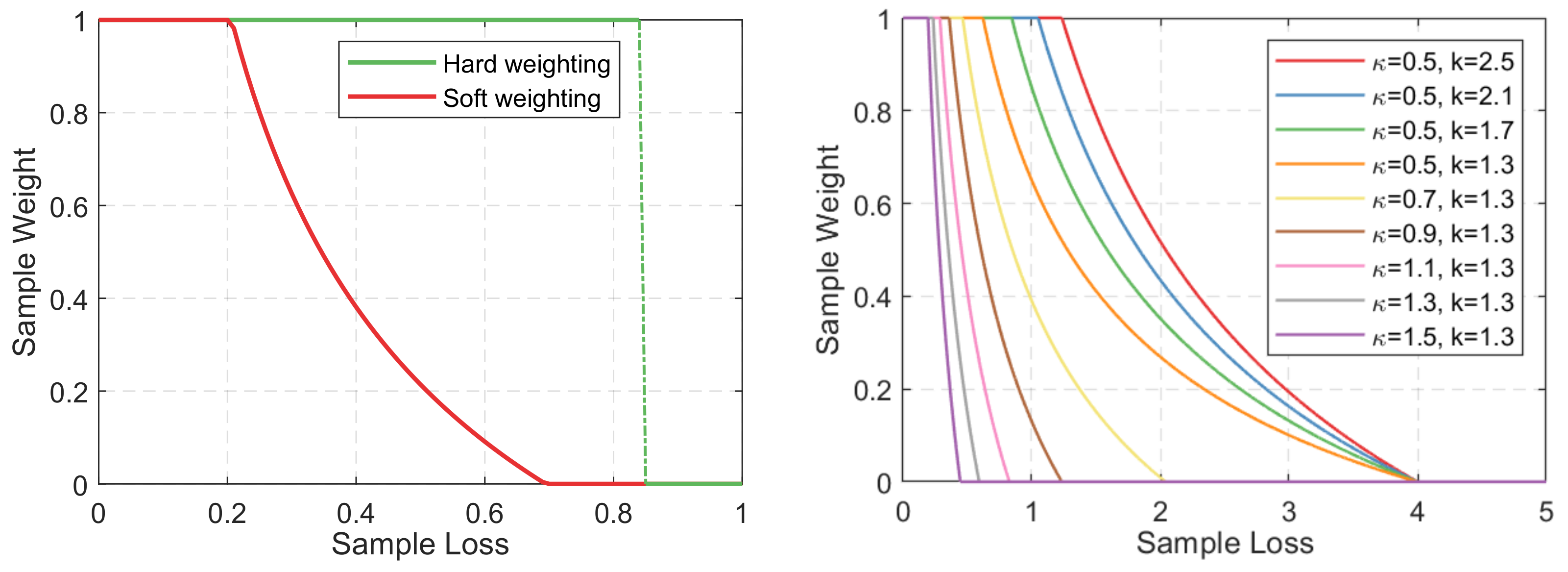
Parameter setting. The issue of point alignment is formulated as the density estimation of the mixture model. However, EM method performs well, as proven in [38]. However, the initial value of the unknown parameter, i.e., the covariances of the Gaussian mixture, would influence the convergence of altering the optimization. Larger σ 2 enables one to filter out many unstable local minimums while decreasing σ 2 , and could obtain a pretty stable local minimum gradually as an iteration. Thus, the deterministic annealing strategy is applied to set a value for σ 2 . We initialize σ 2 with a large value and update it in a fixed annealing rate υ [ 0.9 , 1 ] . Moreover, for an accuracy-aware item, there are some parameters to be set as well, mainly including α , β , η , κ and k. The first three parameters are fixed to 0.1, 2 and 3 as in [28]. For k, κ , we adopt a dynamic assignment strategy instead, directly giving a fixed value. At first, the true matching error is usually large enough for an imprecise T. As iterated, the losses gradually reduce until it converges. So, the weights must change constantly as well for more robust estimation. Specifically, as the loss-weight curves with regards to κ , k are shown in Figure 4, we initialize k, κ with a largish and small value separately. Then, k is gradually reduced to 1.0, and κ is gradually increased until to the preset 1.2 in each iteration.

4.1. Non-Rigid Shape Alignment

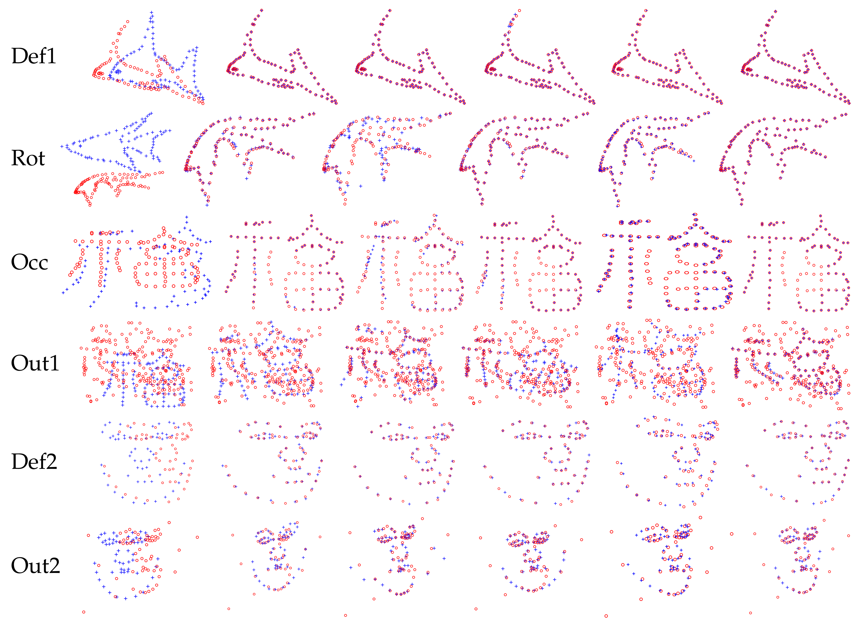
In this experiment, we evaluate the robustness of the presented AA-LMS method on different data degradations, involving deformation, e.g., noise, occlusion, outliers and rotation. Here, the synthesized dataset and IMM Face dataset are selected for testing. The synthesized dataset includes two shape models (fish, Chinese character) with diverse variants, which are the typical 2D shape matching dataset. And, the fish and Chinese character shape sampled from a fish shape and a Chinese character are dispersed as 96 and 108 points, respectively. Meanwhile, the face dataset contains 240 images in total, which are captured from 40 human faces under different face posture. For each face, 58 landmark points are detected to represent the facial contours and the position distribution of facial organs, i.e., nose, eyes and mouth. Due to the change of facial expression, the spatial transformation is non-rigid between the landmark points corresponding to a different face.
Here, six typically shaped data under different deformations are selected to test the proposed method. As shown in Figure 5, the testing data are arranged in the first one for each line, which suffer from complex deformations, i.e., rotation, noise, occlusion and outliers. To quantitatively analyze the performance of our method, four methods are selected to make comparisons, i.e., CPD, L2E, PR-GLS and GCPD. Figure 5 shows the matching results. For the basic fish shape, all the methods are enabled to match satisfactorily. There is a slight offset for the sharp corner when using the PR-GLS method. When the deformation is large, the outliers of all the methods except for ours increase. Since such a sharp part has a larger deformation than other parts, the alignment of such a part would be more intractable. Unlike the fish and Chinese character shape, it is interesting that the face shape is not aligned. There are various micro-expressions for the human face, which leads to many local micro deformations. 58 landmark points are so sparse that the geometric correlation between the adjacent landmark points is pretty weak. Thus, although the landmark points are aligned coarsely, the curves formed by these landmark points are close to each other.
Furthermore, we calculate the root mean square error (RMSE) of the matched points as a numerical measure for the matching error. Table 1 lists the matching errors for different methods on the above shaped data. From the results, our method performs better than other methods. Especially, when there are some local points with complex local character, e.g., inflection, dense or sharp, the proposed method still works well. Actually, these types of points often are the crucial control points for keeping the shape. If they are not aligned well, the global errors would have clear changes. And, such points easily induce the model to strike in a bad local extremum, especially for plenty of outliers or noises. As shown in Figure 5, for the Out2 data, the CPD, L2E and PR-GLS method all converge to the center of outliers in the lower jaw of the face. GCPD method receives a basic alignment except for there being a big deviation on the local parts. However, the proposed method still converges to the true position, which shows the effectiveness of our accuracy-aware mechanism. Note that the soft weight strategy aims to assign real values for each point pair, and the outliers are more likely to be filtered at early iterations, which are unable to influence the later feature matching. After iteration, more faithful points are remained and the final matching becomes more reliable. As a result, our method can work well even if there are plenty of outliers.

4.2. Remote Sensing Image Registration

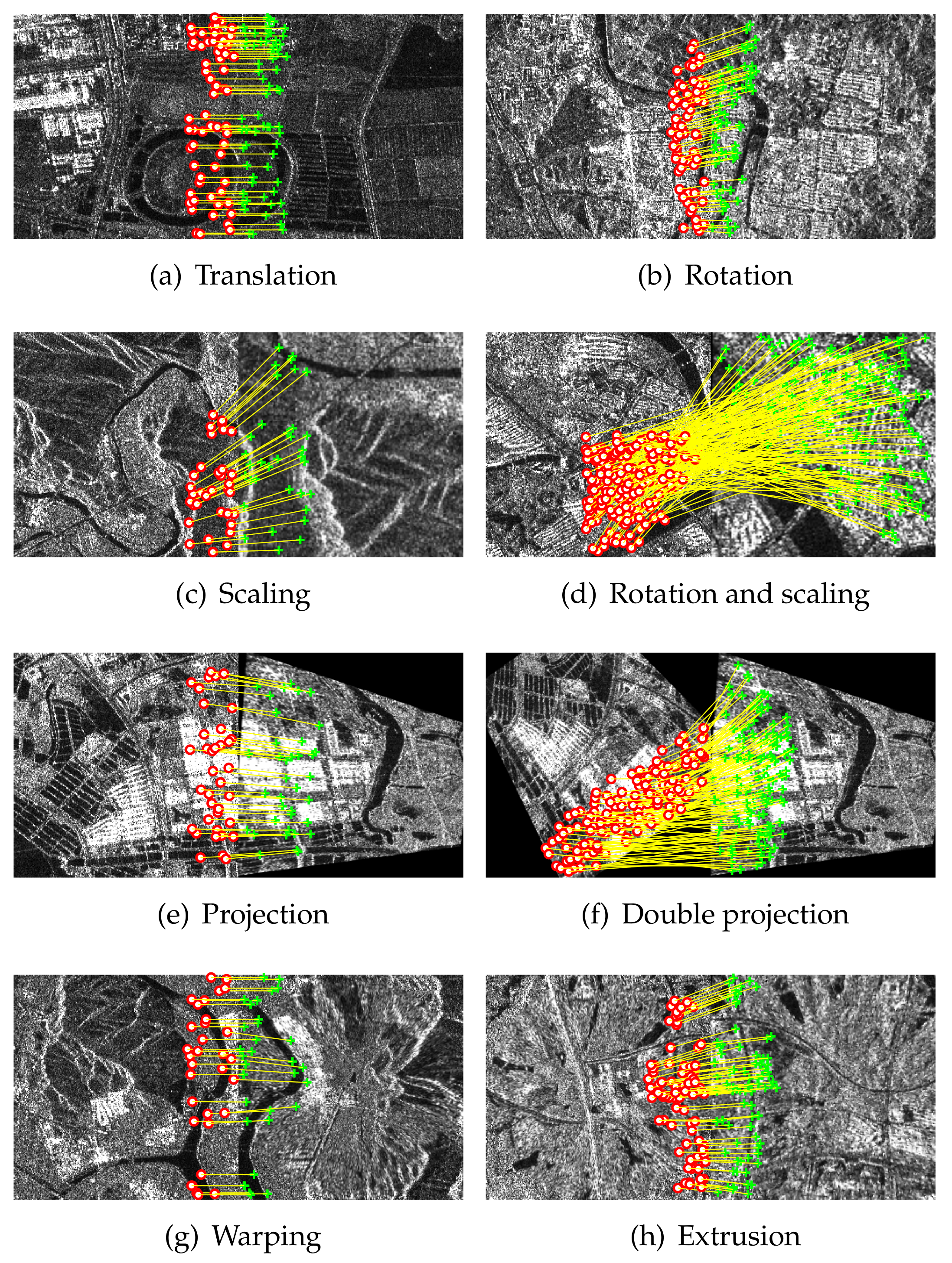
In this section, we employ our method to align the sparse features on real remote sensing images. SARBuD (SAR Building Dataset) [43] is used for testing. This dataset is comprised of medium-high resolution SAR images acquired from GF-3 satellite, which includes the building regions with different terrain scene types, distribution types, and regions. To evaluate the performance of the proposed method, we transform the images with multiple types, such as rotation, scale, projection and warp. And, the proposed method is tested on these image pairs. Figure 6 gives the matching results under different spatial transformations. It is clear that our method enables one to resist geometry deformation. Especially when there is nonlinear deformation in Figure 6g,h, it is still effective. This shows that our method can perform well in both rigid and non-rigid image registration. Although the deformation is complex, our method still obtains many matches, which benefits from the joint optimization for matching error and the number of matched pairs.
To further validate the performance of the proposed method, we employ our method to align remote sensing images under a variety of scenarios. The testing images include hyperspectral image (HSI), multispectral (MSI) and synthetic aperture radar (SAR) images. The data are captured from different scenarios, e.g., space-borne, airborne, and ground-based remote sensing data, which involves various intensity and geometric distortions, As shown in Figure 7, there is obvious nonlinear distortions for image pairs in column 6 and 7 (marked by I 1 , I 2 , , I 7 ). Meanwhile, the objects are similar with each other as well, which makes it easy to bring about many mismatches during recovering correspondences. The image pair I 1 I 7 are acquired at a different time, where there is a significant difference in image intensity, rotation and view. The first four pairs of images are all real remote sensing images from Landsat or unmanned aerial vehicle.
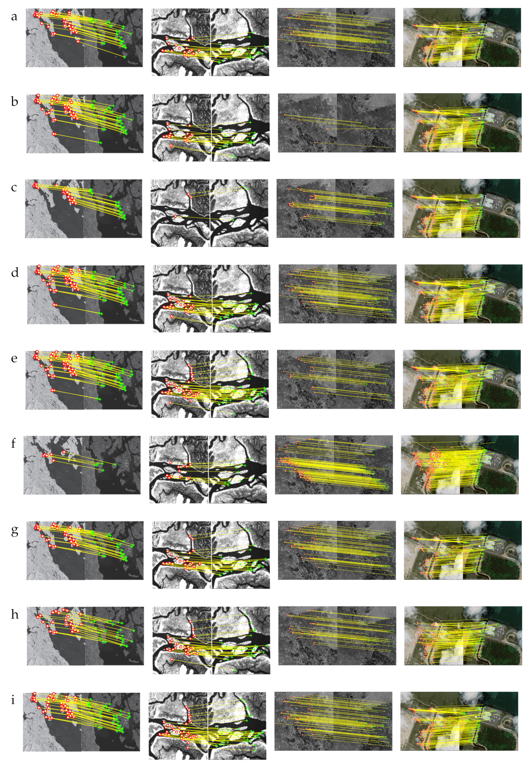
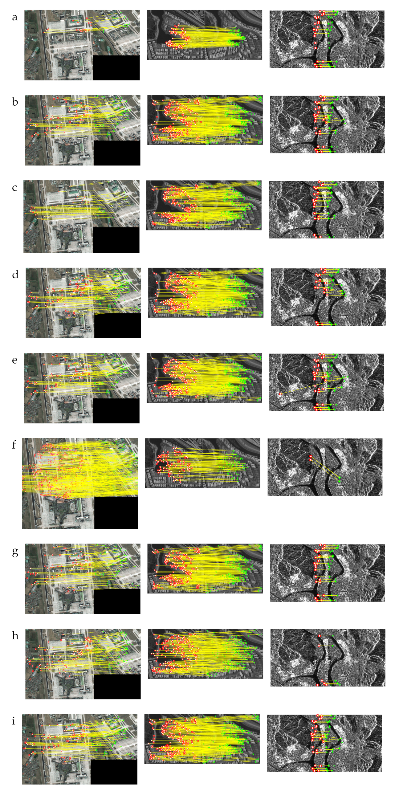
Now, we will register the above pairs of remote sensing images. Whereas the Scale-invariant feature transform (SIFT) [44] is an effective method for feature point detection and has excellent performance in a real scenario, the feature points are detected by the SIFT method in this experiment. Specifically, we first detect SIFT feature points on each pair of the testing remote sensing images, and the initial correspondences can also be established to initialize the testing methods using SIFT. With such initialization, the convergence would be faster. More correct correspondences should determine as many as possible while the outliers presented in initial correspondences are removed as well. Besides CPD, L2E, PR-GLS, DFM, LAF, GCPD and PSC, the common random sample consensus (RANSAC) method is used for evaluation, which performs well in obtaining a consistent matching pair and has been widely applied in the feature matching field. However, it only enables one to find the matching pairs according to one type of spatial transformation. For the image registration with multiple local spatial transformations, it is always incomplete.
Figure 8 gives the feature point matching results on the testing image data under different degradations. As discussed above, the RANSAC method can obtain the matching pairs with high consistency, which causes a local match to be obtained. When the geometry deformation is large, the proposed method can acquire significant matches as compared to RANSAC, CPD, L2E, PR-GLS and LAF, as well as the PSC method. Although GCPD can obtain enough matches, there are some matches lost when the feature points are very close to their adjacent ones. And, the points with minuscule deviations in position are selected as the final true matches, which is similar to CPD, L2E, PR-GLS, LAF and PSC. For the images with rich texture, it is mentionable that DFM obtains quite a number of point pairs, which owes to its vast feature points detected during feature extraction compared to the SIFT method. But, for SAR images, DFM performs poorly. However, with the select weights, the minuscule deviations could be enlarged so that they are easily identified in our method. Meanwhile, the optimization to the matching number ensures that enough matches are obtained using our method. To further analyze this situation, we calculate the matching errors and matching number. As shown in Figure 9, it is clear that our method has a lower root mean square error than others. For the quartus image pair, RANSAC obtains a lower accuracy. However, more matching pairs are lost according to the feature point matching figure, especially for the aircraft parking region with large deformation. Less matched point pairs in the large deformation region mean the final registration is more unstable. As a result, our method performs better in both the matching error and matching number.
Besides the above experiments, more complex situations are tested. The remote sensing images with nonlinear deformations are used to evaluate the effectiveness. We also make comparisons with the state-of-the-art methods such as RANSAC, CPD, L2E, PR-GLS and GCPD. Similarly, the RMSE value is calculated and the correct matches are counted. According to Figure 10, RANSAC tends to find the correspondences around rigid parts. When the input images suffer from badly local distortions, it only obtains a part of correspondences. Compared to RANSAC, CPD, L2E, PR-GLS, LAF, GCPD and PSC methods enable one to determine the correct matches over the non-rigid region. And, the number of matched feature points is also sufficient. However, the false matches are also remained, e.g., the result of PR-GLS on the image pair I 5 and GCPD on the image pair I 7 . In terms of finding consistent feature pairs, the PSC method can work well. But, it also lost more matches. Although the registration of images with nonlinear deformation is difficult, our method still obtains the stable matches even if the non-rigid deformation is large. This shows that our accuracy-aware mechanism is effective for outliers removed, which makes the model tend towards more reliable points. Meanwhile, the dynamic updating strategy makes the model explore more matches.
Table 2 presents the RMSE values of different methods on the testing images under non-rigid deformations and also records the number of features point-matched (#Matches). Although the DFM method based on the deep feature obtains more matches, the matching errors are indeed larger since the accuracy of the feature points are weak; the distributions of feature points by DFM are uneven and agglomerate, which leads to the weak accuracy of the feature points in positioning. Clearly, our method has a lower matching error on the testing image I 5 and I 6 . Although the RMSE value is less than 1, it is larger than that of RANSAC. Note that RANSAC only obtains the matched feature points according with linear deformations and none are determined in the non-rigid deformation located at the center of the overlapping region between the two images. So, it is impossible to align the non-rigid region using the parameters estimated by the RANSAC method. However, it is easy to align the region with the non-rigid deformation using the matched points. Using the spatial transformation model estimated via our method, the matching error is less than 1, which shows the strong fitting ability of our model to the nonlinear deformation. From the number of matched point pairs, our method can explore more matches from the initial correspondences and outperforms others, which is owing to the combination of minimizing the matching error and maximizing the matching number in our model. At the same time, this also shows that it is effective for optimizing the matching number, which is just different from the existing methods.

5. Conclusions

In this paper, we propose a robust AA-LMM method for remote sensing image registration. An accuracy-aware mechanism is designed for guiding the model towards more reliable sample points during matching, which is further formulated as a soft-weighted piece-wise function. With such a special function, the matching error and matching number are fused into a new model and optimized synchronously. To solve the model effectively, with the faithful samples, a sparse approximation with a low-rank constrain is introduced to linearize the model and approach the real deformations by several iterations. Experiments on the public datasets for non-rigid point registration and real remote sensing image data demonstrate that our method can achieve a higher registration accuracy and obtain more matches than the state-of-the-art approaches.
Whereas there is a lot of uncertain factors in the imaging environment, the appearance of image pairs taken in such conditions would be inconsistent in texture, color and gray-scale, etc. It is still full of challenges to align images under various conditions. To deal with these changes, we proposed an accuracy-aware mechanism to select faithful points. However, this selection mechanism is based on accurate numerical computation, which is also eventually effected by dynamical scenarios. So, more strategies for uncertainty calculation would be introduced into our model for the future. For example, such a selection mechanism can work by picking the top certain percentage according to the matching errors sorted in ascending order. Moreover, robust feature extraction is also crucial and we will consider that the features are simultaneously detected on the image pair in a mutual guide manner and focus on the cross-supervised feature extraction network to selectively extract the features from the sub blocks of the input image pairs instead of the whole image.

Author Contributions

Conceptualization, J.Y. and X.L.; methodology, J.Y.; software, J.Y. and C.L.; validation, J.Y.; formal analysis, investigation, J.Y. and X.L.; writing—original draft preparation, J.Y. All authors have read and agreed to the published version of the manuscript.

Funding

This research was supported by the National Natural Science Foundation of China under Grant 61871470.

Data Availability Statement

The 2D shape-matching dataset, IMM Face dataset and SARBuD dataset are publicly available from [41,43].

Conflicts of Interest

The authors declare no conflict of interest.

Abbreviations

The following abbreviations are used in this manuscript:
SLAMSimultaneous localization and mapping
PSRPoint set registration
GMMsGaussian Mixture Models
GMMGaussian Mixture Model
TPSThin plate spline
CPDCoherent points drift
ICPIterative closest point
KCKernel correlation
UAVUnmanned Aerial Vehicle
SARSynthetic aperture radar
HSIHyperspectral image
MSIMultispectral image
RKHSReproducing kernel Hilbert space
RANSACRandom sample consensus
SIFTScale-invariant feature transform
DADeterministic annealing
EDEigen-decomposition
EMExpectation Maximization
RMSERoot mean square error

References

  1. Huang, C.; Mees, O.; Zeng, A.; Burgard, W. Visual language maps for robot navigation. In Proceedings of the IEEE International Conference on Robotics and Automation, London, UK, 29 May–2 June 2023; pp. 10608–10615. [Google Scholar]
  2. Cattaneo, D.; Vaghi, M.; Valada, A. Lcdnet: Deep loop closure detection and point cloud registration for lidar slam. IEEE Trans. Robot. 2022, 38, 2074–2093. [Google Scholar] [CrossRef]
  3. Liu, Y.; Pang, C.; Zhan, Z.; Zhang, X.; Yang, X. Building change detection for remote sensing images using a dual-task constrained deep siamese convolutional network model. IEEE Geosci. Remote Sens. Lett. 2020, 18, 811–815. [Google Scholar] [CrossRef]
  4. Xiang, Y.; Wang, F.; You, H. OS-SIFT: A robust SIFT-like algorithm for high-resolution optical-to-SAR image registration in suburban areas. IEEE Geosci. Remote Sens. 2018, 56, 3078–3090. [Google Scholar] [CrossRef]
  5. Balakrishnan, G.; Zhao, A.; Sabuncu, M.R.; Guttag, J.; Dalca, A.V. VoxelMorph: A learning framework for deformable medical image registration. IEEE Trans. Med. Imaging 2019, 38, 1788–1800. [Google Scholar] [CrossRef]
  6. Yang, K.; Pan, A.; Yang, Y.; Zhang, S.; Ong, S.H.; Tang, H. Remote sensing image registration using multiple image features. Remote Sens. 2017, 9, 581. [Google Scholar] [CrossRef]
  7. Shen, Z.; Han, X.; Xu, Z.; Niethammer, M. Networks for joint affine and non-parametric image registration. In Proceedings of the IEEE/CVF Conference on Computer Vision and Pattern Recognition, Los Angeles, CA, USA, 16–20 June 2019; pp. 4224–4233. [Google Scholar]
  8. Liu, S.; Yang, B.; Wang, Y.; Tian, J.; Yin, L.; Zheng, W. 2D/3D multimode medical image registration based on normalized cross-correlation. Appl. Sci. 2022, 12, 2828. [Google Scholar] [CrossRef]
  9. Paul, S.; Pati, U.C. A comprehensive review on remote sensing image registration. Int. J. Remote Sens. 2021, 42, 5396–5432. [Google Scholar] [CrossRef]
  10. Han, L.; Xu, L.; Bobkov, D.; Steinbach, E.; Fang, L. Real-time global registration for globally consistent rgb-d slam. IEEE Trans. Robot. 2019, 35, 498–508. [Google Scholar] [CrossRef]
  11. Chui, H.; Rangarajan, A. A new point matching algorithm for non-rigid registration. Comput. Vis. Image Underst. 2003, 89, 114–141. [Google Scholar] [CrossRef]
  12. Maiseli, B.; Gu, Y.; Gao, H. Recent developments and trends in point set registration methods. J. Vis. Commun. Image Represent. 2017, 46, 95–106. [Google Scholar] [CrossRef]
  13. Jian, B.; Vemuri, B.C. Robust point set registration using gaussian mixture models. IEEE Trans. Pattern Anal. Mach. Intell. 2010, 33, 1633–1645. [Google Scholar] [CrossRef] [PubMed]
  14. Fan, J.; Yang, J.; Ai, D.; Xia, L.; Zhao, Y.; Gao, X.; Wang, Y. Convex hull indexed Gaussian mixture model (CH-GMM) for 3D point set registration. Pattern Recognit. 2016, 59, 126–141. [Google Scholar] [CrossRef]
  15. Yang, Y.; Ong, S.H.; Foong, K.W.C. A robust global and local mixture distance based non-rigid point set registration. Pattern Recognit. 2015, 48, 156–173. [Google Scholar] [CrossRef]
  16. Ma, J.; Zhao, J.; Ma, Y.; Tian, J. Non-rigid visible and infrared face registration via regularized Gaussian fields criterion. Pattern Recognit. 2015, 48, 772–784. [Google Scholar] [CrossRef]
  17. Wang, G.; Zhou, Q.; Chen, Y. Robust non-rigid point set registration using spatially constrained Gaussian fields. IEEE Trans. Image Process. 2017, 26, 1759–1769. [Google Scholar] [CrossRef]
  18. Tajdari, F.; Huysmans, T.; Song, Y. Non-rigid registration via intelligent adaptive feedback control. IEEE Trans. Vis. Comput. Graph. 2023, 1–17. [Google Scholar] [CrossRef]
  19. Schölkopf, B.; Herbrich, R.; Smola, A.J. A generalized representer theorem. In Proceedings of the International Conference on Computational Learning Theory, Amsterdam, The Netherlands, 16–19 July 2001; pp. 416–426. [Google Scholar]
  20. Guo, Y.; Zhao, L.; Shi, Y.; Zhang, X.; Du, S.; Wang, F. Adaptive weighted robust iterative closest point. Neurocomputing 2022, 508, 225–241. [Google Scholar] [CrossRef]
  21. Cao, L.; Zhuang, S.; Tian, S.; Zhao, Z.; Fu, C.; Guo, Y.; Wang, D. A Global Structure and Adaptive Weight Aware ICP Algorithm for Image Registration. Remote Sens. 2023, 15, 3185. [Google Scholar] [CrossRef]
  22. Ma, J.; Ma, Y.; Zhao, J.; Tian, J. Image feature matching via progressive vector field consensus. IEEE Signal Process. Lett. 2014, 22, 767–771. [Google Scholar] [CrossRef]
  23. Li, X.; Ma, Y.; Hu, Z. Rejecting mismatches by correspondence function. Int. J. Comput. Vis. 2010, 89, 1–17. [Google Scholar] [CrossRef]
  24. Myronenko, A.; Song, X. Point set registration: Coherent point drift. IEEE Trans. Pattern Anal. Mach. Intell. 2010, 32, 2262–2275. [Google Scholar] [CrossRef]
  25. Tsin, Y.; Kanade, T. A correlation-based approach to robust point set registration. In Proceedings of the European Conference on Computer Vision, Prague, Czech Republic, 11–14 May 2004; pp. 558–569. [Google Scholar]
  26. Tang, J.; Shao, L.; Zhen, X. Robust point pattern matching based on spectral context. Pattern Recognit. 2014, 47, 1469–1484. [Google Scholar] [CrossRef]
  27. Qu, H.B.; Wang, J.Q.; Li, B.; Yu, M. Probabilistic model for robust affine and non-rigid point set matching. IEEE Trans. Pattern Anal. Mach. Intell. 2016, 39, 371–384. [Google Scholar] [CrossRef] [PubMed]
  28. Ma, J.; Zhao, J.; Yuille, A.L. Non-rigid point set registration by preserving global and local structures. IEEE Trans. Image Process. 2015, 25, 53–64. [Google Scholar]
  29. Wang, J.; Chen, J.; Xu, H.; Zhang, S.; Mei, X.; Huang, J.; Ma, J. Gaussian field estimator with manifold regularization for retinal image registration. Signal Process. 2019, 157, 225–235. [Google Scholar] [CrossRef]
  30. Huang, X.; Zhang, J.; Fan, L.; Wu, Q.; Yuan, C. A systematic approach for cross-source point cloud registration by preserving macro and micro structures. IEEE Trans. Image Process. 2017, 26, 3261–3276. [Google Scholar] [CrossRef]
  31. Fan, J.; Cao, X.; Yap, P.T.; Shen, D. BIRNet: Brain image registration using dual-supervised fully convolutional networks. Med. Image Anal. 2019, 54, 193–206. [Google Scholar] [CrossRef] [PubMed]
  32. Hansen, L.; Heinrich, M.P. GraphRegNet: Deep graph regularisation networks on sparse keypoints for dense registration of 3D lung CTs. IEEE Trans. Med. Imaging 2021, 40, 2246–2257. [Google Scholar] [CrossRef]
  33. Arar, M.; Ginger, Y.; Danon, D.; Bermano, A.H.; Cohen-Or, D. Unsupervised multi-modal image registration via geometry preserving image-to-image translation. In Proceedings of the IEEE/CVF Conference on Computer Vision and Pattern Recognition, Seattle, WA, USA, 16–20 June 2020; pp. 13410–13419. [Google Scholar]
  34. Mok, T.C.; Chung, A. Fast symmetric diffeomorphic image registration with convolutional neural networks. In Proceedings of the IEEE/CVF Conference on Computer Vision and Pattern Recognition, Seattle, WA, USA, 16–20 June 2020; pp. 4644–4653. [Google Scholar]
  35. Goforth, H.; Lucey, S. GPS-denied UAV localization using pre-existing satellite imagery. In Proceedings of the International Conference on Robotics and Automation, Montreal, QC, Canada, 20–24 May 2019; pp. 2974–2980. [Google Scholar]
  36. Papadomanolaki, M.; Christodoulidis, S.; Karantzalos, K.; Vakalopoulou, M. Unsupervised multistep deformable registration of remote sensing imagery based on deep learning. Remote Sens. 2021, 13, 1294. [Google Scholar] [CrossRef]
  37. Xu, Y.; Li, J.; Du, C.; Chen, H. NBR-Net: A nonrigid bidirectional registration network for multitemporal remote sensing images. IEEE Trans. Geosci. Remote Sens. 2022, 60, 1–15. [Google Scholar] [CrossRef]
  38. Horaud, R.; Forbes, F.; Yguel, M.; Dewaele, G.; Zhang, J. Rigid and articulated point registration with expectation conditional maximization. IEEE Trans. Pattern Anal. Mach. Intell. 2010, 33, 587–602. [Google Scholar] [CrossRef]
  39. Yuille, A.L.; Grzywacz, N.M. A computational theory for the perception of coherent visual motion. Nature 1988, 333, 71–74. [Google Scholar] [CrossRef]
  40. Micchelli, C.A.; Pontil, M.; Bartlett, P. Learning the Kernel Function via Regularization. J. Mach. Learn. Res. 2005, 6, 1099–1125. [Google Scholar]
  41. Zheng, Y.; Doermann, D. Robust point matching for nonrigid shapes by preserving local neighborhood structures. IEEE Trans. Pattern Anal. Mach. Intell. 2006, 28, 643–649. [Google Scholar] [CrossRef]
  42. Nordstrøm, M.M.; Larsen, M.; Sierakowski, J.; Stegmann, M.B. The IMM Face Database—An Annotated Dataset of 240 Face Images; Technical University of Denmark: Lyngby, Denmark, 2004. [Google Scholar]
  43. Wu, F.; Zhang, H.; Wang, C.; Li, L.; Li, J.J.; Chen, W.R.; Zhang, B. SARBuD1.0: A SAR Building Dataset Based on GF-3 FSII Imageries for Built-up Area Extraction with Deep Learning Method. Natl. Remote Sens. Bull. 2022, 26, 620–631. [Google Scholar] [CrossRef]
  44. Lowe, D.G. Distinctive image features from scale-invariant keypoints. Int. J. Comput. Vis. 2004, 60, 91–110. [Google Scholar] [CrossRef]
  45. Ma, J.; Qiu, W.; Zhao, J.; Ma, Y.; Yuille, A.L.; Tu, Z. Robust L2E estimation of transformation for non-rigid registration. IEEE Trans. Signal Process. 2015, 63, 1115–1129. [Google Scholar] [CrossRef]
  46. Fan, A.; Ma, J.; Tian, X.; Mei, X.; Liu, W. Coherent point drift revisited for non-rigid shape matching and registration. In Proceedings of the IEEE/CVF Conference on Computer Vision and Pattern Recognition, New Orleans, LA, USA, 19–23 June 2022; pp. 1424–1434. [Google Scholar]
  47. Efe, U.; Ince, K.G.; Alatan, A. Dfm: A performance baseline for deep feature matching. In Proceedings of the IEEE/CVF Conference on Computer Vision and Pattern Recognition, Online, 19–25 June 2021; pp. 4284–4293. [Google Scholar]
  48. Jiang, X.; Ma, J.; Fan, A.; Xu, H.; Lin, G.; Lu, T.; Tian, X. Robust feature matching for remote sensing image registration via linear adaptive filtering. IEEE Trans. Geosci. Remote Sens. 2020, 59, 1577–1591. [Google Scholar] [CrossRef]
  49. Xia, Y.; Jiang, J.; Lu, Y.; Liu, W.; Ma, J. Robust feature matching via progressive smoothness consensus. ISPRS J. Photogramm. Remote Sens. 2023, 196, 502–513. [Google Scholar] [CrossRef]
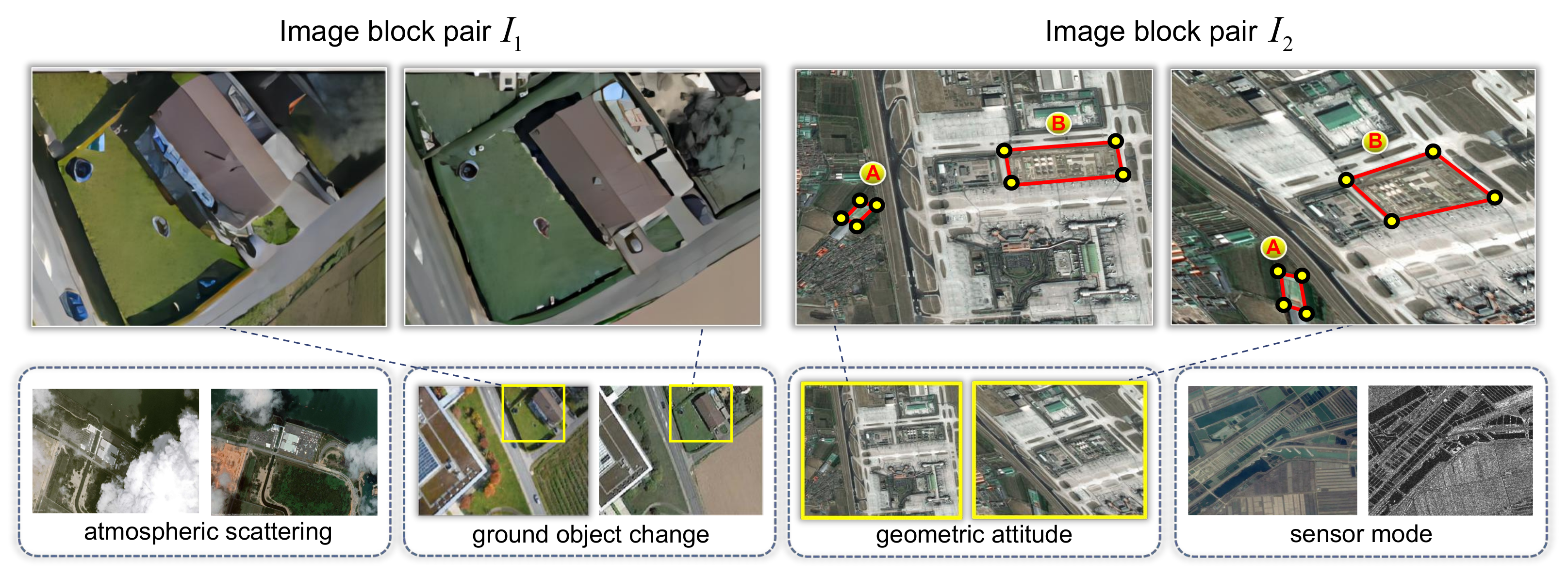
Figure 1. Some examples of remote sensing images with typical deformations are caused by various factors, such as atmospheric scattering, ground object change, and geometric attitude, as well as the mode of the imaging sensor.
Remotesensing 15 05314 g001
Figure 2. The matched feature point pairs with different accuracy of localization. The local image block in each image shows the feature points detected on the image. The feature points detected on the input image pair are marked by green plus sign and red circle, respectively. The blue arrow shows the points are corresponding.
Remotesensing 15 05314 g002
Figure 3. The overview of the proposed AA-LMM registration method for remote sensing images. The soft selection and basis function expression are fused into the least square registration error model. The new objective function involves both registration error and the number of feature point pairs matched, which are linearized via low-rank approximation during alternative optimization. The green plus sign and red circle denote the feature points detected on each input image pair, respectively.
Remotesensing 15 05314 g003
Figure 4. Hard- and soft-weighting manner. The left shows a comparison for soft curve ( κ = 1 , k = 1.2 ) with hard one. The figure on the right shows that the curves of weights change as the matching loss changes under different parameter κ , k. From the weight curves, the upper and lower abrupt point of the curve are determined by κ , k, which determines the tolerance for the matching error.
Remotesensing 15 05314 g004
Figure 5. Schematic results for CPD, L2E, PR-GLS, GCPD and our method. The test data with deformation, noise, outliers and rotation presented in every two rows is denoted as Def1, Rot, Out1, Def2 and Out2 with blue ‘+’ and red ‘o’ from top to bottom. For each line, the first figure is the model and data point sets, and the subsequent figures are the registration results of CPD, L2E, PR-GLS, GCPD and ours.
Remotesensing 15 05314 g005
Figure 6. Registration results of the proposed method on SAR image data under different spatial deformations: translation, rotation, scaling, projection and extrusion. The green plus sign and red circle denote the feature points detected on each input image pair, respectively.
Remotesensing 15 05314 g006
Figure 7. Examples of the testing remote sensing image pairs under different spatial deformation.
Remotesensing 15 05314 g007
Figure 8. The matching results of different methods on real remote sensing images under various deformations. (ai) denote the results of RANSAC, CPD, L2E, PR-GLS, GCPD, DFM, LAF, PSC and ours, respectively. The feature points detected on each image are marked by green plus sign and red circle, respectively.
Remotesensing 15 05314 g008
Figure 9. The comparisons of matching error and matching number for different methods on the testing remote sensing image pairs under different spatial deformation.
Remotesensing 15 05314 g009
Figure 10. The comparisons of matching error and matching number for RANSAC, CPD, L2E, PR-GLS, GCPD, DFM, LAF, PSC and ours (marked by (ai)) on real remote sensing images with complex deformations. The feature points detected on each image are marked by green plus sign and red circle, respectively.
Remotesensing 15 05314 g010
Table 1. Comparisons of the matching errors for different methods on the synthesized and IMM Face datasets. The bold matching errors denote the best score and performance.
MethodsDef1RotOccOut1Def2Out2
CPD0.26240.26730.00501.13791.55710.1267
L2E0.00430.01290.01400.78950.69390.0306
PR-LGS0.01660.00320.00460.68820.52590.0255
GCPD0.00810.00400.08960.51530.50300.0151
Ours0.00450.00100.00140.50530.48760.0097
Table 2. Comparisons of the matching errors and the number of matched feature point pairs for different methods on the remote sensing images with local non-rigid deformation.
MethodMetrics#Matches
I 5 I 6 I 7 I 5 I 6 I 7
RANSAC1.45410.81980.39592413727
CPD2.39800.91671.71198634930
L2E2.59012.73532.93145525022
PR-GLS2.21002.83411.55899931923
GCPD2.40332.07862.60158329231
DFM13.29014.893-8611243
LAF4.34782.42552.59529633830
PSC9.13142.4650.2877872856
Ours1.44650.79450.513510636931
Disclaimer/Publisher’s Note: The statements, opinions and data contained in all publications are solely those of the individual author(s) and contributor(s) and not of MDPI and/or the editor(s). MDPI and/or the editor(s) disclaim responsibility for any injury to people or property resulting from any ideas, methods, instructions or products referred to in the content.