Abstract
Geological hazards often occur in mountainous areas and are sudden and hidden, so it is important to identify and assess geological hazards. In this paper, the western mountainous area of Beijing was selected as the study area. We conducted research on landslides, collapses, and unstable slopes in the study area. The surface deformation of the study area was monitored by multi-temporal interferometric synthetic aperture radar (MT-InSAR), using a combination of multi-looking point selection and permanent scatterer (PS) point selection methods. Random forest (RF), support vector machine (SVM), convolutional neural network (CNN), and recurrent neural network (RNN) models were selected for the assessment of geological hazard susceptibility. Sixteen geological hazard-influencing factors were collected, and their information values were calculated using their features. Multicollinearity analysis with the relief-F method was used to calculate the correlation and importance of the factors for factor selection. The results show that the deformation rate along the line-of-sight (LOS) direction is between −44 mm/year and 28 mm/year. A total of 60 geological hazards were identified by combining surface deformation with optical imagery and other data, including 7 collapses, 25 unstable slopes, and 28 landslides. Forty-eight of the identified geological hazards are not recorded in the Beijing geological hazards list. The most effective model in the study area was RF. The percentage of geological hazard susceptibility zoning in the study area is as follows: very low susceptibility 27.40%, low susceptibility 28.06%, moderate susceptibility 21.19%, high susceptibility 13.80%, very high susceptibility 9.57%.
1. Introduction
The occurrence of geological hazards poses great danger; for example, landslides and debris flows have led to a large number of deaths and significant economic and property losses [1,2]. On steep slopes in mountainous areas, a series of geological hazards can be triggered by large-scale movements of water, sediments, and other materials [3]. The interferometric synthetic aperture radar (InSAR) technique can obtain surface deformation information and is an effective means to assist in the identification of geological hazards. Geological hazard susceptibility assessments can be used as a reference for relevant researchers and are an important part of geological hazard prevention and control [4].
InSAR is characterized by a wide spatial coverage, a high monitoring accuracy and all-weather monitoring, making it an important technology for geological hazard monitoring and identification [5,6,7,8]. Differential InSAR (D-InSAR) was extended from InSAR technology to allow for deformation monitoring [9]. MT-InSAR can overcome the effects of D-InSAR by spatial and temporal incoherence, as well as atmospheric effects, and acquires a long time series of deformation in the target area. Additionally, the monitoring accuracy technology has been able to reach millimeter level [10]. Geological hazards will be accompanied by a certain degree of surface deformation before and after the occurrence of geological hazards. Therefore, the identification, monitoring, and assessment of geological hazards can be carried out in conjunction with surface deformation monitoring using the MT-InSAR technology. Nowadays, MT-InSAR techniques, such as PS-InSAR [11], SBAS-InSAR [12], and SqueeSAR [13], are widely used in the monitoring and identification of geological hazards such as landslides, unstable slopes, and so on.
Geological hazard susceptibility assessment is an evaluation of the ease of occurrence of geological hazards in the study area [14]. The spatial distribution of geological hazards can follow complex patterns, depending on the spatial variability of a large number of predisposing factors. Geological hazard susceptibility assessment is the use of data or expert experience to find patterns in the distribution of geological hazards in a certain area [15]. Geological hazard susceptibility assessments can be mainly categorized into qualitative methods and quantitative methods [16,17]. Qualitative methods are mostly based on experience, such as the analytic hierarchy process (AHP) method [18], historical geological hazard inventory analysis [19], and expert scoring methods [20]. These methods are simple and cost-effective, but less objective and only suitable for the analysis of smaller study areas [21]. With the development of geographic information data and computer technology, quantitative methods have gradually become the mainstream method in the assessment of geological hazards [22]. Quantitative methods are able to utilize the relationship between data and geological hazards for susceptibility assessments, which is more objective and accurate than qualitative methods, as these mainly include statistical methods and artificial intelligence methods. There are many statistically based methods of susceptibility assessment, such as the information value method, the frequency ratio method, the coefficient of determination method, and the weights of evidence method [23,24,25]. Artificial intelligence methods can learn the deep features of geological hazards and reveal the nonlinear change characteristics of geological hazards: for example, machine learning methods such as logistic regressions [26], support vector machine [27], and random forest [28], and the deep learning methods such as deep neural network [29], convolutional neural network [30], and recurrent neural network [31]. There are now many reliable methods for assessing geological hazard susceptibility, so many researchers have studied the comparison of the effectiveness of different models. However, in different studies, different regions and data lead to different model effects, so it is necessary to select multiple models for comparison when conducting a geological hazard susceptibility study in a certain region.
This paper will focus on the MT-InSAR geological hazard identification study and the comparison of different geological hazard susceptibility assessment models. This study takes the western mountainous area of Beijing, where geological hazards are frequently developed, as the study area [32]. We will conduct research on landslides, collapses, and unstable slopes in the study area. Firstly, surface deformation information for the study area, from September 2016 to September 2022, was extracted using the MT-InSAR to identify geological hazards. Collecting geological hazard influencing factors was undertaken for the geological hazard susceptibility assessment, using identified and historical geohazards as samples. Finally, the geological hazard susceptibility was assessed using the RF, SVM, CNN, and RNN models, and the effectiveness of each model was compared, to achieve a reasonable and reliable geological hazard susceptibility assessment. This study provides a reference for the study of geological hazards in the mountainous areas of western Beijing, as well as for the study of susceptibility assessment model options.
2. Study Area and Datasets
2.1. Study Area
As shown in Figure 1a,c, the study area is in Fangshan District and Mentougou District, Beijing, China (115.561838°–115.999379°E and 39.700610°–40.020247°N) and covers an area of 1328 km2. The area is located in the northeastern section of the Taihang Mountains, so the geomorphology is dominated by mountains and the elevation is mainly between 36 m and 2036 m. The age stratigraphy of the study area is fully developed. The diaphanous fold in which the study area is located is part of the Yanshan platform fold belt, and the geological and tectonic changes in the study area mainly occurred in the Indo-Chinese and Yanshan periods.
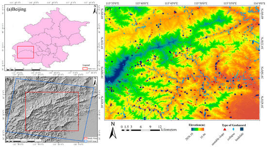
Figure 1.
(a) Location of the study area in Beijing. (b) SAR data coverage. (c) Elevation and historical geological hazards in the study area.
The main geological structures in the study area are folds, large fractures, and general fractures. The study area has a continental monsoon climate, the area below 1000 m is a warm temperate climate zone, and the area above 1000 m is a cold temperate climate zone, due to the influence of the topography. There is a large temperature difference between different areas at different times, with more precipitation in summer and less precipitation in winter, and overall uneven precipitation throughout.
The occurrence of geological hazards in the study area is mainly influenced by the complex topographic and geological conditions in the study area, the existence of fracture structures, the large amount of precipitation during the rainy season, and the frequent human engineering activities. The main types of geological hazards in the study area are collapses, landslides, and unstable slopes, the distributions of which are shown in Figure 1c. The characteristics of these geological hazards are as follows [33,34]:
- Collapses: Collapses are usually sudden in nature; some have no significant deformation in the InSAR deformation results. In optical images, the contour line of the collapse body is obvious; its color is related to the lithology, which is usually lighter in tone than the surrounding, as mostly gray or grayish white. The collapse body is piled up on the bottom of slopes with a bumpy surface. Sometimes huge boulders are visible. There is very poor vegetation cover.
- Unstable slopes: Unstable slopes are slopes with large deformation and they are often close to underground resource extraction areas.
- Landslides: The main types of landslides include rotational landslides, translational landslides, and debris flows. The deformation is evident, and a number of typical features can be easily distinguished, like the detachment and accumulation zones, crown, scarp, flank, main body, foot, and toe.
2.2. Datasets
In this study, a total of 80 views of descending track RADARSAT-2 SAR data, from September 2016 to September 2022, were used for MT-InSAR deformation monitoring. As Figure 1b shows, the SAR range fully covers the study area. The RADARSAT-2 SAR data are from a C-band synthetic aperture radar with a wavelength of 5.6 cm and a revisit period of 24 days. The data mode is the Extra Fine mode, offering a resolution of 5 m. The ALOS 12.5 m digital elevation model (DEM) from Japan Aerospace Exploration Agency (JAXA) and precise orbit data were used to remove the flat earth and topographic phases.
The geological hazard data are divided into two parts, one for geological hazards identified by combining surface deformation information, and one for historical geological hazards. The historical geological hazards data are from the geological hazards list for Beijing, published in 2022, including 1034 collapses (71% of the total), 260 unstable slopes (18% of the total) and 158 landslides (11% of the total). A good susceptibility assessment would require us to perform a separate assessment for each type of geological hazards, but also would need a large amount of training data. Therefore, we performed a susceptibility assessment with every type together, in order to have a large number of data; more refined assessments will be the objectives of future works.
Following a review of the relevant literature and considering the topography of the study area, geology, human activities, climate and other factors, 16 geological hazard-influencing factors were selected [35,36,37,38,39]. These included elevation, slope, aspect, plan curvature, profile curvature, topographic wetness index (TWI), topographic roughness index (TRI), slope length and slope angle factor (LS-factor) [40], precipitation, normalized difference vegetation index (NDVI), distance to rivers, distance to roads, landcover, distance to faults, stratigraphic unit, and distance to mine origin. The elevation was determined using 2.5 m resolution DEM data, collected by UAV in 2022 and provided by the Beijing Institute of Geological Hazard Prevention, and the slope, aspect, plan curvature, profile curvature, TWI, TRI, and LS-factor were all also calculated by this DEM. Precipitation was calculated using ERA5 1° resolution atmospheric reanalysis data. NDVI was calculated based on the GEE platform, using 30 m resolution Landsat8 data. The distance to rivers and distance to roads were calculated from road and river vector data, obtained from the OpenStreetMap website. Landcover data were from the ESA WorldCover 10 m resolution landcover data for 2020, released by ESA. Distance to faults and stratigraphic units were obtained from the 1:2,500,000 geological map vector data, 1:1,000,000 geological map vector data, and the 2021 China Mineral Properties Data vector data, respectively, released by the China Geoscientific Data Discovery Publishing System. The distances to the mine origin were obtained from 2021 China Mineral Properties Data vector data, and were defined as the mine origin in a place that had been mined, including both open pit and underground mines. Finally, all raster data with a resolution higher than 30 m were resampled to 30 m, and precipitation data with a resolution lower than 30 m were converted to 30 m by Kriging interpolation. The vector data were converted to 30 m resolution raster data. All data were integrated to construct the dataset.
3. Materials and Methods
3.1. Overview
Figure 2 illustrates the flowchart of this study. Firstly, we used MT-InSAR to obtain the surface deformation of the study area. We combined the PS point selection method and the multi-looking point selection method to select the interferometric points. Then, we used precision orbit data and DEM data for the differential interferometric calculations of surface deformation. The surface deformation consists of linear and nonlinear deformation. After calculating the surface deformation, the geological hazards in the study area were identified based on the rate of surface deformation. We collected geological hazard-influencing factors, combining identified geological hazards and historical geological hazards to create a geological hazards sample, then calculated the information value of the influencing factors. Next, the correlation between the factors was calculated by multiple covariance analysis, and the importance of the factors was calculated by the relief-F method for the selection of influencing factors. Finally, we used the RF, SVM, CNN, and RNN models to assess the geological hazard susceptibility, and compared and analyzed the performance of each model by multiple indicators.
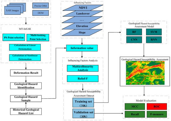
Figure 2.
Flowchart of geological hazard identification and susceptibility assessment.
3.2. MT-InSAR Processing
In this study, an interferometric point target analysis (IPTA) technique was used for surface deformation information extraction. IPTA technology is a MT-InSAR technique that allows the researcher the flexibility to perform baseline combinations, interferometric point selection, and other operations to conduct the study.
3.2.1. Interferometric Point Target Selection
In this study, the amplitude deviation threshold method and the multi-looking point selection method were used to select interferometric point target. The amplitude deviation threshold method is a commonly used method for selecting PS points in MT-InSAR. This method uses the amplitude stability of the image element instead of coherence. In general, the statistical characteristics of the amplitude can only be calculated correctly if the number of images is sufficiently large (≥25). Amplitude deviation can be calculated as follows [41]:
where is the mean of the amplitude and is the variance of the amplitude.
To increase the density of interferometric point targets, we performed multi-looking analysis on the data, with a 3:3 ratio for differential interference and selected all the pixels of the data, after having performed multi-looking, as candidate target points; this approach can reduce the impact of SAR data noise, and differential phases with high coherence can be obtained.
The points selected by the above two methods were fused as candidate coherent points, and these points were masked by a temporal coherence threshold and a standard deviation threshold to obtain the final point target.
3.2.2. Calculation of Linear Deformation
Due to the interference of the coherent point targets of the main image with the coherent point targets of other images, the flat earth phase and terrain phase were then removed by external DEM data. Assuming a total of K sets of interferometric pairs and n coherent point targets are selected, the phase value of point i (1 < i < n) on the kth (1 < k < K) amplitude differential interferogram can be expressed as follows [42]:
where is the unwrapped phase with a value between , is the phase value of the point target, is the deformation phase of the target point due to the change in LOS direction of the satellite during the two imaging sessions of SAR data, is the phase of atmospheric delay due to different atmospheric delays when SAR data were imaged twice, is the noise phase due to random noise in the radar imaging process, is the phase of DEM residuals due to insufficient aging or accuracy of the DEM used for differential interference. The phase of DEM residuals can be expressed in Equation (3) [42]:
where is radar wavelength, is the vertical spatial baseline, is the distance between the radar and the target point, and is the DEM residuals.
The deformation phase can usually be divided into two parts, a part concerned with the linear deformation phase with time, and a part concerned with the nonlinear deformation phase. The deformation phase can be expressed in Equation (4) [42]:
where is the time interval of the interference pair where the target point is located and is the linear deformation rate of the target point.
Errors such as an atmospheric delay phase in the differential interference phase of different interference pairs cannot be calculated using the phase of a single target point. These errors can be calculated at stable target points with high coherence, where the deformation is smaller and less affected by the atmosphere. The errors can be attenuated, and the deformation of the point target can be modeled and solved, by constructing a Delaunay triangular network to connect the high coherence points for quadratic differential calculations. The differential phase between adjacent points in the triangular network can be expressed as follows [42]:
where is the difference in elevation correction values between two target points, is the difference in linear deformation rates between two target points, is the phase residual, and the main components are nonlinear deformation rate, atmospheric delay phase, and noise phase. The closer the distance in space, the higher the atmospheric correlation, so the closer the target points are, and the more similar they are, the more they are affected by the atmosphere and the smaller the atmospheric phase in the differential phase is. In the Delaunay triangular network, the combined target points are limited to a 1 km horizontal distance in space, and the atmospheric phase in the differential phase of the two points is negligible. The linear deformation rate and elevation residuals of each target point are constant across the interference pairs and can be calculated as follows [42]:
From this equation, it can be seen that the relative elevation residuals between the vertical baseline and the two points are linearly related to the corresponding slope, and the time interval of the interference pair is linearly time related to the slope corresponding to the relative deformation velocity. In order to seek the optimal solution for the phase of elevation residuals and the phase of linear deformation, the coherent point targets in the Delaunay triangular network connected by reliable edges can be filtered according to the coherence, and the coherence function model is as follows [42]:
where is an imaginary unit. The value of this function is one when the coherent point target is completely uncorrelated, and zero in the case of complete decoherence. After screening the coherent point targets with a good quality according to the coherence, a coherent point was selected as the reference point, to calculate the linear deformation phase, and elevation residuals were solved on each connected edge of the triangular network, as follows [42]:
where m is the number of points connected to the interference point target. The equation for calculating the elevation residuals is the same as this equation.
3.2.3. Calculation of Nonlinear Deformation
After calculating the linear deformation phase and the elevation residual phase in the differential interference phase of the coherent point target, the nonlinear deformation phase was also calculated. The nonlinear deformation phase is present in the phase residual of the coherent point target, which consists of the nonlinear deformation phase, the atmospheric delay phase, and the noise phase. The main components of the phase residuals are as follows [42]:
The three components of the phase residuals have different spatial–temporal characteristics, and they can be extracted based on their spatial-temporal distribution characteristics. The influence of the troposphere is different at different moments, so the influence of atmospheric delay on the radar signal at different moments during interference is also different, causing the atmospheric delay phase to have a high correlation in space and be a low-frequency signal, but to be random in time and be a high-frequency signal. The nonlinear deformation is a low-frequency signal in time and a high-frequency signal with randomness in space. The phase noise is random in space and time.
The atmospheric phase of each view image affects each interference pair in which that view image is located. In order to calculate the atmospheric delay phase for each interferometric pair, the atmospheric phase of the main image needed to be calculated. The baseline combination chosen in this study was a multi-master image approach. Considering that each scene image is involved in several sets of differential interference, the time average of the interferometric atmospheric phase of multiple interferometric pairs can be regarded as an approximation of the atmospheric phase of the main image, as follows [42]:
Then, the atmospheric phase in the differential interference phase of each interference pair can be calculated as follows [42]:
where is a low-pass spatial filter, and is a high-pass time filter. denotes the atmospheric delay phase of the point target in the main image, meaning that high-pass filtering can eliminate the effect of nonlinear distortion and obtain the atmospheric delay phase with the noise phase in the slave image of the kth interference pair, and that low-pass filtering of the results will obtain the atmospheric phase of the slave image. The atmospheric phases of the master and slave image were then summed to give the complete atmospheric phase of the interference pair. Finally, the nonlinear deformation phase was obtained by removing the atmospheric phase in , and low-pass filtering to remove the noise phase, as follows [42]:
Finally, the nonlinear deformation phase was added to the linear phase to achieve the complete deformation information of the target at the coherent point.
3.3. Geological Hazard Susceptibility Assessment Method
3.3.1. Influencing Factors Selection
- Information Value Model
The information value model can calculate the information value of the influencing factors using the spatial relationship between the geological hazards and the influencing factors. The information value can reflect the level of the contribution of the influencing factors to the occurrence of the hazards. In this study, the influencing factors were reclassified, and the information value of each classification of each influencing factor was used as the features of geological hazards, so as to improve the accuracy and efficiency of the geological hazard susceptibility evaluation model.
For geological hazard , is each classification of each influencing factor (i is the number of influencing factors, is the number of subclasses of each influencing factor). The information value can be expressed as in Equation (13) [15]:
where is the probability of geological hazard occurrence in the area of , and is the probability of geological hazard occurrence in the whole study area.
Since it was difficult to express the probability of the occurrence of geological hazards in this study, the probability was calculated based on the number of geological hazard grids as follows [15]:
In Equation (14), is the information value of , is the number of geological hazard grids in the area of , is the number of grids in the area of . is the number of geological hazard grids in the whole study area, and is the number of grids in the whole study area.
- 2
- Multicollinearity Analysis
Multicollinearity analysis can be used to calculate the correlation between influencing factors. Multicollinearity means that at least two influencing features are highly correlated linearly. In this study, tolerance level (TOL) and variance inflation factor (VIF) were used for the evaluation. For the independent variable data set, i.e., the influencing factors , the VIF value was calculated as follows [43]:
where is the correlation coefficient of the regression equation, fitted with the influencing factor as the dependent variable, and the rest of the influencing factors are the independent variables.
The value of TOL is the reciprocal of VIF. In general, if VIF < 10 (TOL > 0.1), the influencing factors are considered to be independent of each other, they can all be used for geological hazard susceptibility evaluation, and there is no collinearity.
- 3
- Relief-F
The relief feature selection (relief-F) method can be used to calculate the relative importance of the influencing factors to geological hazard occurrence. The relief-F algorithm evaluates the importance of a feature’s ability to discriminate in a classification task as an evaluation factor, by calculating the degree of difference between factors in the same class of nearest-neighbor samples and in different classes of nearest-neighbor samples. For the input sample set , we randomly selected a sample , then selected the same-category nearest-neighbor sample set and the non-category nearest-neighbor sample set of sample . The weight of the influencing factor can be expressed as follows [44]:
where is the probability of the class , is the class of , is the jth sample of class , and is the difference between different samples on an influencing factor. After repeating this process m times, the weights can be calculated.
3.3.2. Geological Hazard Susceptibility Assessment Models
- RF
Random forest (RF) is an algorithm that assembles multiple decision trees through an ensemble learning approach [45]. The random forest model consists of several decision trees and uses the Bagging model to take multiple independent samples from the total sample as the training dataset, which are then fed into the decision tree for classification. The Bagging method draws samples randomly and with put-back, as an independent training set, and builds a decision tree for each extracted training set separately. Finally, the decision results of each decision tree are combined for voting, resulting in the optimal classification result.
In this study, we used python to complete the RF model, based on the random forest classifier in the Scikit-learn framework.
- 2
- SVM
The support vector machine (SVM) model is a supervised machine learning model. SVM takes the training error as the constraint of the optimization problem and minimizes the confidence interval as the optimization objective [46]. The basic principle of SVM is to map the sample data to a high-dimensional space and find the optimal hyperplane in that space to partition the different classes of data. In this process, the model finds a set of support vectors that are the closest data points to the hyperplane. This hyperplane separates the data points of the two categories and uses the maximum interval to improve the classification accuracy. Based on this principle, the SVM model is suitable for two-class classification problems such as geological hazard susceptibility evaluation where both positive and negative samples exist.
In this study, we used python to complete the SVM model based on the support vector machine classifier in the Scikit-learn framework.
- 3
- CNN
Convolutional neural network (CNN) models are feedforward neural networks with a deep structure that can be computed by convolving data. In this study, 1D-CNN architectures were used. In addition to the input and output layers, as in a normal neural network, the network structure also includes two convolutional layers, one pooling layer, and two fully connected layers [47].
The convolution kernel in the convolution layer can be regarded as a regular shaped filter. The convolution window slides over the input data set and sums the inner product of its fixed weights with the data inside the window. The convolution kernel outputs convolutional features after completing one convolution operation on the entire input data, namely the primary features extracted by the convolution operation. The pooling layer is used to achieve the sampling of features, which can reduce the amount of data used while retaining useful information, preventing over-fitting, and improving the generalization ability of the model. The fully connected layer can map high-dimensional features extracted by convolution and pooling operations to a low-dimensional feature space. We extract the geological hazard features by convolution and pooling operations, and then reorganize them by a fully connected layer. Finally, we let the fully connected layer be connected to the output layer, which consists of two neurons representing geological hazards and non-geological hazards.
In this study, the CNN model was implemented in python under the Tensorflow framework, and included two convolutional layers, a maxpool layer, a flattened layer, two fully connected layers and a dropout layer between the fully connected layers.
- 4
- RNN
A recurrent neural network (RNN) is a neural network that recurses the input sequence data in the direction of the data over the sequence and is able to chain all nodes together [48]. Unlike other neural networks, RNN can use serialized information, and it can capture dynamic information in serialized data by periodically connecting hidden layer nodes. Each unit in the RNN is associated with other units in the hidden layer at different time intervals, so that information can be passed from one layer to the next in the network. In 2020, Wang Yi et al. experimentally demonstrated that inputting the influencing factors into the RNN model according to their importance can effectively improve the performance of the RNN model for geological hazard susceptibility assessment [18]. Therefore, we ranked the importance of the factors according to the relief-f method, constructed the sequence data based on the importance ranking of the factors, and input them into the RNN model for the evaluation of geohazard susceptibility.
In this study, the RNN model was implemented in Python under the Tensorflow framework and included a simple RNN layer and a fully connected layer.
3.3.3. Model Evaluation
Five randomly selected training and validation sets were put into a 7:3 ratio for cross-validation. The training set is inputted into the geological hazard susceptibility assessment model for training, and the validation set is classified and evaluated for accuracy using the trained model receiver operating characteristic (ROC) curve, which can effectively indicate the predictive power of different geological hazard susceptibility assessments [49]. In this study, ROC curves were used to assess model effectiveness by calculating area under the curve (AUC) values, in order to compare different models’ predictive abilities. In addition, three indicators, namely the recall, F-score, and Matthews correlation coefficient (MCC), are used to compare different models’ accuracy [14]:
4. Results
4.1. Deformation Results from MT-InSAR
In this study, the IPTA technique uses small baseline ideas for interferometric pair combining, in order to reduce the effect caused by spatial–temporal incoherence and improve the interferometric quality. Due to the time interval of the data being stabilized and the addition of precision orbital data, there is no spatial–temporal baseline threshold set during the combination of interferometric pairs, and the main image of the data of each view is combined with the data of the following two views, forming a total of 157 interferometric pairs, as shown in Figure 3a.
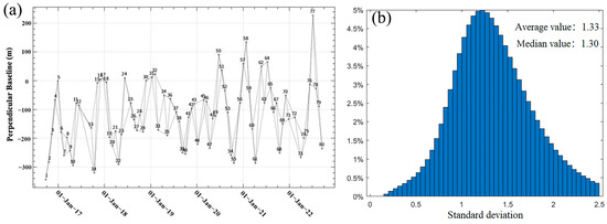
Figure 3.
(a) Spatial-temporal baseline of the interferogram. (b) Histogram of standard deviation of all points.
We set the amplitude deviation threshold to 1.25 for point selection, then combined it with the points selected by the multi-looking method, and finally calculated the temporal coherence of all the points, keeping the points with temporal coherence greater than 0.7 as monitoring points. A total of 1,418,107 points were finally selected. Figure 4a shows the annual average surface deformation rate along the radar line of direction of sight of the study area, from September 2016 to September 2022, acquired by the MT-InSAR technique mentioned in Section 3.2. The figure shows that most of the study area was in a stable state, and the maximum deformation rate was −44 mm/year. Figure 3b shows a histogram of the standard deviation for all points, with an average value of 1.33, which proves the reliability of the monitoring points.
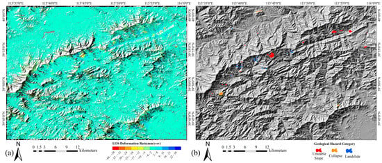
Figure 4.
(a) LOS deformation rate in study area. (b) Distribution of identified geological hazards.
4.2. Geological Hazard Identification
In this study, we combine InSAR deformation results, UAV imagery, and Google Earth data for geological hazard identification. The identified geological hazards were mainly classified into three categories: collapses, unstable slopes, and landslides. The principles for identifying geological hazards were as follows:
- Using 10 mm/year as the threshold [50], we selected the areas where deformation points with deformation greater than this threshold gathered, and considered these areas as deformation areas;
- Using orthophoto images generated by UAV, Google Earth, we considered the terrain, topography, and spectral, textural, topographical, and morphological features of the deformation area to confirm whether it was a geological hazard. Finally, we classified geological hazards [34];
- At this point, there were still geological hazards that could not be identified by deformation. Supplementary identification was carried out, based on optical images, topography, and the distribution of historical geological hazards.
As shown in Figure 4b, a total of 60 geological hazard areas were identified, with 7 collapses, 25 unstable slopes, and 28 landslides, of which 12 were on the geological hazards list as existing geological hazards. Several typical geological hazards in the study area are shown in Figure 5.

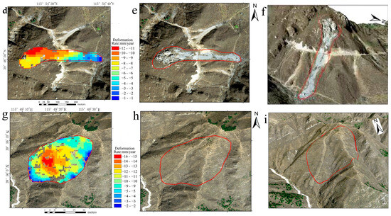
Figure 5.
Deformation rate image (a), 2D image (b), and 3D image (c) of landslide. Deformation rate image (d), 2D image (e), and 3D image (f) of collapse. Deformation rate image (g), 2D image (h), and 3D image (i) of unstable slope.
4.3. Geological Hazard Susceptibility Assessment
We combined the identified geological hazards and the geological hazards in the geological hazards list to create the sample of geological hazards. All the grids where the geological hazard samples were located were used as positive samples. We selected the same number of non-geological hazard grids as negative samples. The information value of each influencing factor was calculated, as shown in Table A1 and Figure A1.
Table 1 presents the analysis of covariance between the influencing factors. It can be observed that all correlation coefficients are below 0.7 and the VIF values of these factors are below five (TOL > 0:2). Figure A2 shows the correlations between the factors, all of which are less than 0.5. Therefore, all the factors are independent of each other and there is no covariance between them. Figure 6a shows the importance of each influencing factor, as calculated by the relief-F method, and it can be seen that the importance of the influencing factors is positive, i.e., all the influencing factors contribute to the occurrence of geological disasters to a certain extent. Among them, the stratigraphic unit factor and the road distance factor have a higher importance to the occurrence of geological hazards. In summary, all influencing factors can participate in the vulnerability assessment.

Table 1.
Multicollinearity analysis results for landslide-influencing factors.

Figure 6.
(a) Multicollinearity analysis results for influencing factors. (b) ROC curves for four models.
We inputted the influencing factors as the features, the information values as the features value, and whether or not the feature was a geological hazard as a label into the model for training and used the trained model to predict the probability of each grid being a geological hazard, which was then used as the susceptibility index for that grid. The models’ parameter settings are shown in Table 2. Then, the susceptibility of all grids was reclassified into five classes, using the natural breaks method, as follows: very high susceptibility, high susceptibility, moderate susceptibility, low susceptibility, and very low susceptibility. Figure 7a–d shows the results of the susceptibility assessment of the four methods; as can be seen from the figure, the distribution and pattern of susceptibility zones derived from the four methods are relatively similar. Table 3 shows the correlation of geological hazard susceptibility derived from each model, from which it can be seen that there is a strong correlation between all models. The accuracy and runtime of the four models are shown in Table 4 and the ROC curves and AUC of the four models are shown in Figure 6b. All four models achieved good prediction accuracy, with the RF model having the highest AUC value and the shortest runtime.

Table 2.
Parameter settings of the models.
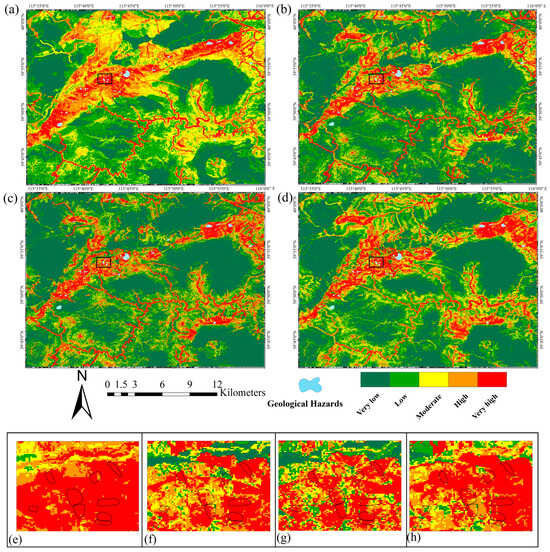
Figure 7.
Geological hazard susceptibility assessment results of RF (a), SVM (b), CNN (c), and RNN (d). Comparison of small areas of RF (e), SVM (f), CNN (g), and RNN (h).

Table 3.
Correlations of susceptibility across models.

Table 4.
Performances of different models.
We calculated statistics regarding the number of grids of geological hazard susceptibility zones derived from the four models, and regarding the number of grids of geological hazards in those susceptibility zones. As shown in Figure 8, most of the susceptibility zones derived from the four models were in the very low susceptibility and low susceptibility zones, and most of the geological hazard grids were within the very high susceptibility and high susceptibility zones. As can be seen in Figure 7e–h and Figure 8, the RF model zoning results had the lowest percentage of geological hazard grids within the low and very low susceptibility zones and the highest percentage of geological hazard grids within the high and very high susceptibility zones; the susceptibility zoning decreases in steps from low to high, which was mostly consistent with the distribution of geological hazard susceptibility [51]. Therefore, the RF model was considered to be the best model for the geological hazards susceptibility assessment in the study area, and the results were as follows: very low susceptibility 27.40%, low susceptibility 28.06%, moderate susceptibility 21.19%, high susceptibility 13.80%, and very high susceptibility 9.57%.
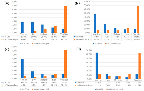
Figure 8.
Percentage of grids in susceptibility zones and grids of geological hazards within zones derived from the models of RF (a), SVM (b), CNN (c), and RNN (d).
5. Discussion
In this study, we used MT-InSAR, combined with PS point selection and multi-looking point selection, to improve the density of the monitoring points. We also obtained denser monitoring points for surface deformation monitoring in the mountainous areas of western Beijing with high vegetation cover. We evaluated the accuracy using the statistical standard deviation, which proved the reliability of the method to improve the density of monitoring points.
From the identification results, MT-InSAR was more effective in identifying slow-moving geological hazards, such as landslides and unstable slopes, and less effective in identifying faster-moving geological hazards, such as collapses. Geological hazards in the study area were distributed in a regular pattern, with many points and small surfaces. Most of the geological hazards on the list were found by manual surveys, and they were distributed near roads, making it easier to find hazards related to human activities and those that were a greater threat to people’s lives and safety. MT-InSAR can be used to find hazards in more hidden areas that are difficult for surveyors to reach, such as valleys and mining areas. This proves the reliability of MT-InSAR technology for geological hazard identification, as it was more comprehensive than manual surveys.
Although there are differences in the triggering mechanisms and characteristics of different types of geological hazards, there are still common characteristics in their spatial distribution. The models in this study were assessed for multiple types of geological hazards and reliable results were obtained. This demonstrates that the models used in the study can all learn the common characteristics of multiple types of geological hazard. The occurrence process of geological hazards is more complicated, and there are many assessment methods. Many scholars have already compared different susceptibility assessment models to select the most suitable model for the study area [52,53]. The results show that all models can perform effective geological hazard susceptibility assessments. The RF model worked better than the other three models, yielding a less noisy and smoother susceptibility map with a more reasonable percentage of susceptibility partitions. Additionally, the RNN model was far quicker than other models in terms of runtime. Although the model accuracy of the CNN model was high, its zoning results were biased towards bipolarity, which was not in line with the geological hazard zoning rule. This is due to the variety of geological hazards in the geological hazard samples used, and in the sample added to the historical geological hazards, resulting in geological hazards of a large time span, which in turn resulted in noise in the data samples. Relative to the scope of the study area, the number of samples of geological hazards was small, and the deep learning model found it difficult to effectively learn the characteristics of geological hazards. The RF model, with the characteristics of multi-model decision-making, is very good at overcoming these problems.
6. Conclusions
In this paper, we mainly carried out geological hazard identification and susceptibility assessments, and effectiveness evaluations of different models in the western mountainous area of Beijing. Two main results were obtained, as follows:
First, a combination of multi-looking point selection and PS point selection was used to increase the density of MT-InSAR monitoring points and obtain surface deformation information about the study area, and the accuracy of this method was demonstrated by counting the standard deviation of the monitoring points. The study area was found to be essentially in a steady state, with a maximum deformation rate of −44 mm/year. Based on surface deformation information combined with optical images, 60 geological hazards were identified in the study area, with 7 collapses, 25 unstable slopes, and 28 landslides.
Second, the identified and historical geological hazards were combined as geological hazard samples, and the geological hazard influencing factors were collected. They were analyzed as the features of the geological hazards, and their information values were analyzed as the feature values. The factor selection was carried out, using multicollinearity analysis and the relief-F method. The results showed that 16 influence factors could all be used for the geological hazard susceptibility assessments; among these, roads and stratigraphic units had the greatest impact on geological hazards. Finally, the geological hazard susceptibility assessment results were obtained using different models for comparison. All models achieved reliable results, with the RF model performing best. This demonstrates the great advantage of RF models in learning multi-class and long time-span geological hazard characteristics. Additionally, the percentages of geological hazard susceptibility zoning in the study area were as follows: very low susceptibility 27.40%, low susceptibility 28.06%, moderate susceptibility 21.19%, high susceptibility 13.80%, and very high susceptibility 9.57%.
The research in this paper has significance for future research on surface deformation, the distribution of geological hazards, and the assessment of geological hazard susceptibility in the mountainous areas of western Beijing, and also provides a reference for the prevention and control of geological hazards in Beijing and the whole North China region. The methodology of this paper can also be used as a reference for MT-InSAR surface deformation monitoring or geological hazard susceptibility assessment model selection in similar study areas. Future research can be conducted regarding three aspects: (1) research on the automatic identification of geological hazards can be carried out based on optical images, deformation rates, and differential phases, and automatic geological hazard identification can improve the efficiency of geological hazard identification. (2) Dynamic assessment of geological hazard susceptibility, when combined with precipitation, soil moisture, seasons and other dynamic factors, can more accurately identify geological hazard-prone areas and provide references for geological hazard prevention and control. (3) Refined assessment of the susceptibility of different types of geological hazards, as their characteristics are not identical. A good susceptibility assessment requires that each type be assessed separately.
Author Contributions
All authors contributed to the study conception and design. Z.L. and H.Y. conceived of the original idea and structure of this paper. Z.L. collected data and completed the experiment. Z.L. wrote the manuscript and Y.W. reviewed the manuscript. W.Z. and P.L. provided critical comments in planning this paper. All authors have read and agreed to the published version of the manuscript.
Funding
This research was funded by Beijing Key Laboratory of Urban Spatial Information Engineering (No. 20220102).
Data Availability Statement
Data are contained within the article.
Acknowledgments
The authors would like to thank the Japan Aerospace Exploration Agency for providing ALOS DEM data, the Beijing Institute of Geological Hazard Prevention for providing DOM and DEM of UAV and historical geological hazards data and the China Geological Survey for geological data. In addition, thanks to Google Earth, OpenStreetMap data and the ESA WorldCover dataset.
Conflicts of Interest
The authors declare no conflict of interest.
Appendix A

Table A1.
Information values of geological hazard-influencing factors.
Table A1.
Information values of geological hazard-influencing factors.
| Factor | Factor Class | No. of Grids | % of Grids | Geohazard Grids | Geohazard Grids(%) | Information Value |
|---|---|---|---|---|---|---|
| Elevation (m) | 36–322 | 209,817 | 14.21% | 1113 | 15.52% | 0.088047 |
| 323–607 | 493,627 | 33.43% | 2121 | 29.57% | −0.122668 | |
| 608–893 | 458,644 | 31.06% | 1642 | 22.89% | −0.305135 | |
| 894–1179 | 220,270 | 14.92% | 1295 | 18.06% | 0.190881 | |
| 1180–1465 | 70,910 | 4.80% | 956 | 13.33% | 1.020815 | |
| 1466–1750 | 17,422 | 1.18% | 43 | 0.60% | −0.677065 | |
| 1751–2036 | 5779 | 0.39% | 2 | 0.03% | −2.641615 | |
| Slope (rad) | 0–0.27 | 250,062 | 16.94% | 1132 | 15.78% | −0.070538 |
| 0.28–0.54 | 540,151 | 36.58% | 2909 | 40.56% | 0.103146 | |
| 0.55–0.81 | 591,174 | 40.04% | 2879 | 40.14% | 0.002517 | |
| 0.82–1.08 | 90,736 | 6.15% | 248 | 3.46% | −0.575096 | |
| 1.09–1.35 | 4288 | 0.29% | 4 | 0.06% | −1.650096 | |
| Aspect | Flat (−1) | 917 | 0.06% | 0 | 0.00% | 0 |
| North (337.5°–22.5°) | 186,881 | 12.66% | 644 | 8.98% | −0.382895 | |
| Northeast (22.5°–67.5°) | 193,637 | 13.11% | 690 | 9.62% | −0.309825 | |
| East (67.5°–112.5°) | 198,927 | 13.47% | 913 | 12.73% | −0.056733 | |
| Southeast (112.5°–157.5°) | 199,209 | 13.49% | 913 | 12.73% | −0.05815 | |
| South (157.5°–202.5°) | 182,796 | 12.38% | 1010 | 14.08% | 0.128804 | |
| Southwest (202.5°–247.5°) | 169,656 | 11.49% | 1077 | 15.02% | 0.267631 | |
| West (247.5°–292.5°) | 167,063 | 11.32% | 1081 | 15.07% | 0.28674 | |
| Northwest (292.5°–337.5°) | 177,383 | 12.01% | 844 | 11.77% | −0.02069 | |
| Plan Curvature | −0.027–0.0049 | 116,417 | 7.88% | 412 | 5.74% | −0.316689 |
| −0.0048–−0.0014 | 330,995 | 22.42% | 1701 | 23.72% | 0.056334 | |
| −0.0013–0.0015 | 561,709 | 38.04% | 2940 | 40.99% | 0.074647 | |
| 0.0016–0.005 | 331,235 | 22.43% | 1628 | 22.70% | 0.011746 | |
| 0.0051–0.026 | 136,108 | 9.22% | 491 | 6.85% | −0.297538 | |
| Profile Curvature | −0.025–−0.005 | 109,963 | 7.45% | 825 | 11.50% | 0.434706 |
| −0.004–−0.002 | 332,736 | 22.54% | 1957 | 27.29% | 0.191285 | |
| −0.001–0.001 | 611,892 | 41.44% | 2869 | 40.00% | −0.035371 | |
| 0.002–0.005 | 317,488 | 21.50% | 1292 | 18.01% | −0.177027 | |
| 0.006–0.071 | 104,385 | 7.07% | 229 | 3.19% | −0.794898 | |
| TWI | 1.7–5 | 733,943 | 49.71% | 2972 | 41.44% | −0.181972 |
| 2.1–6.9 | 458,604 | 31.06% | 2734 | 38.12% | 0.204803 | |
| 7–9.6 | 190,190 | 12.88% | 846 | 11.80% | −0.088035 | |
| 9.7–13.8 | 73,221 | 4.96% | 422 | 5.88% | 0.170992 | |
| 13.9–24.3 | 20,510 | 1.39% | 198 | 2.76% | 0.686823 | |
| TRI | 0–6.8 | 229,329 | 15.53% | 1171 | 16.33% | 0.049212 |
| 6.9–12.7 | 533,731 | 36.15% | 3036 | 42.33% | 0.157161 | |
| 12.8–18.6 | 514,331 | 34.84% | 2422 | 33.77% | −0.031761 | |
| 18.7–28.8 | 170,129 | 11.52% | 483 | 6.73% | −0.537784 | |
| 28.9–107.9 | 27,898 | 1.89% | 60 | 0.84% | −0.815454 | |
| LS-Factor | 0–18.1 | 501,137 | 33.94% | 2041 | 28.46% | −0.176255 |
| 18.2–144.6 | 959,959 | 65.02% | 4948 | 68.99% | 0.059278 | |
| 144.7–488.1 | 13,703 | 0.93% | 139 | 1.94% | 0.736289 | |
| 488.2–1554.7 | 1512 | 0.10% | 43 | 0.60% | 1.767196 | |
| 1554.8–4609.9 | 99 | 0.01% | 1 | 0.01% | 0.732065 | |
| Precipitation (m) | 0–100 | 117,012 | 7.93% | 123 | 1.72% | −1.572805 |
| 100–200 | 258,261 | 17.49% | 1006 | 14.03% | −0.262946 | |
| 200–500 | 353,546 | 23.95% | 1273 | 17.75% | −0.341595 | |
| 500–1000 | 335,283 | 22.71% | 2284 | 31.85% | 0.295996 | |
| 1000–2000 | 412,367 | 27.93% | 2795 | 38.97% | 0.290961 | |
| NDVI | −0.41–0.04 | 1329 | 0.09% | 0 | 0.00% | 0 |
| −0.03–0.19 | 37,393 | 2.53% | 337 | 4.70% | 0.618068 | |
| 0.2–0.32 | 64,701 | 4.38% | 935 | 13.04% | 1.090239 | |
| 0.33–0.41 | 219,242 | 14.85% | 1365 | 19.03% | 0.248202 | |
| 0.42–0.47 | 563,527 | 38.17% | 2490 | 34.72% | −0.094708 | |
| 0.48–0.55 | 502,529 | 34.04% | 1588 | 22.14% | −0.429954 | |
| 0.56–0.84 | 87,748 | 5.94% | 457 | 6.37% | 0.069683 | |
| Distance to Road (m) | 0–100 | 189,712 | 12.85% | 2167 | 30.21% | 0.851954 |
| 100–200 | 136,799 | 9.27% | 422 | 5.88% | −0.457145 | |
| 200–500 | 307,285 | 20.81% | 1082 | 15.09% | −0.324847 | |
| 500–1000 | 346,864 | 23.49% | 2659 | 37.07% | 0.453135 | |
| 1000–2000 | 349,585 | 23.68% | 630 | 8.78% | −0.994665 | |
| >2000 | 148,622 | 10.07% | 246 | 3.43% | −1.079712 | |
| Distance to River (m) | 0–100 | 58,036 | 3.93% | 538 | 7.50% | 0.646264 |
| 100–200 | 54,507 | 3.69% | 268 | 3.74% | 0.012127 | |
| 200–500 | 143,741 | 9.74% | 313 | 4.36% | −0.802341 | |
| 500–1000 | 196,071 | 13.28% | 449 | 6.26% | −0.751985 | |
| 1000–2000 | 317,163 | 21.48% | 1766 | 24.62% | 0.136525 | |
| >2000 | 706,951 | 47.88% | 3838 | 53.51% | 0.111214 | |
| Landcover | Tree cover | 894,102 | 60.56% | 3496 | 48.75% | −0.218287 |
| Shrubland | 62 | 0.00% | 0 | 0.00% | 0 | |
| Grassland | 474,735 | 32.15% | 2700 | 37.65% | 0.158476 | |
| Cropland | 24,995 | 1.69% | 72 | 1.00% | −0.51801 | |
| Built-up | 49,604 | 3.36% | 404 | 5.63% | 0.514295 | |
| Bare | 29,827 | 2.02% | 500 | 6.97% | 1.164069 | |
| Water | 2248 | 0.15% | 0 | 0.00% | 0 | |
| Stratigraphic Unit | C | 207,927 | 14.08% | 715 | 9.97% | −0.387618 |
| J | 259,323 | 17.56% | 470 | 6.55% | −1.028055 | |
| Jx | 582,921 | 39.48% | 4786 | 66.73% | 0.482686 | |
| O | 62,197 | 4.21% | 302 | 4.21% | −0.042593 | |
| P | 71,121 | 4.82% | 676 | 9.43% | 0.629097 | |
| Qb | 161,641 | 10.95% | 245 | 3.42% | −1.206833 | |
| Qp | 129,310 | 8.76% | 287 | 4.00% | −0.825443 | |
| ∈ | 2029 | 0.14% | 0 | 0.00% | 0 | |
| Distance to Fault (m) | 0–100 | 44,805 | 3.03% | 311 | 4.34% | 0.383891 |
| 100–200 | 45,550 | 3.09% | 268 | 3.74% | 0.218595 | |
| 200–500 | 130,518 | 8.84% | 922 | 12.86% | 0.401452 | |
| 500–1000 | 199,420 | 13.51% | 1464 | 20.41% | 0.439933 | |
| 1000–2000 | 348,381 | 23.60% | 1848 | 25.77% | 0.114981 | |
| >2000 | 707,827 | 47.94% | 2359 | 32.89% | −0.349788 | |
| Distance to Mine Origin (m) | 0–100 | 9670 | 0.65% | 152 | 2.12% | 1.201271 |
| 100–200 | 25,462 | 1.72% | 375 | 5.23% | 1.136157 | |
| 200–500 | 120,030 | 8.13% | 1146 | 15.98% | 0.702709 | |
| 500–1000 | 251,046 | 17.00% | 1528 | 21.31% | 0.252497 | |
| 1000–2000 | 483,530 | 32.75% | 2685 | 37.44% | 0.160741 | |
| >2000 | 627,062 | 42.47% | 1286 | 17.93% | −0.835335 |

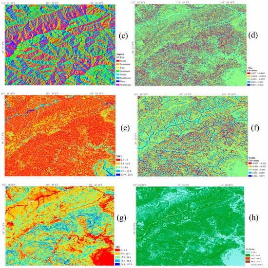
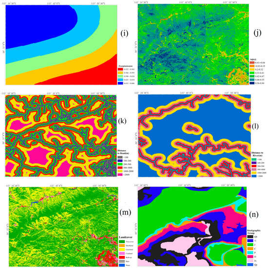
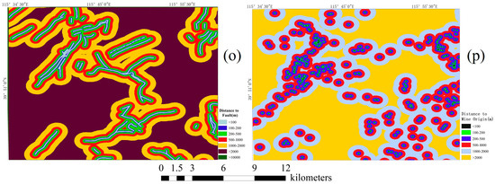
Figure A1.
(a) Elevation. (b) Slope. (c) Aspect. (d) Plan curvature. (e) TWI. (f) Profile curvature. (g) TRI. (h) LS-Factor. (i) Precipitation. (j) NDVI. (k) Distance to road. (l) Distance to river. (m) Landcover. (n) Stratigraphic unit. (o) Distance to fault. (p) Distance to mine origin.
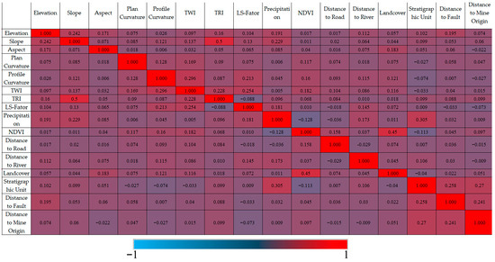
Figure A2.
Influencing factors’ correlation matrix.
References
- Dowling, C.A.; Santi, P.M. Debris flows and their toll on human life: A global analysis of debris-flow fatalities from 1950 to 2011. Nat. Hazards 2014, 71, 203–227. [Google Scholar] [CrossRef]
- Gatto, A.; Clò, S.; Martellozzo, F.; Segoni, S. Tracking a Decade of Hydrogeological Emergencies in Italian Municipalities. Data 2023, 8, 151. [Google Scholar] [CrossRef]
- Coussot, P.; Meunier, M. Recognition, classification and mechanical description of debris flows. Earth-Sci. Rev. 1996, 40, 209–227. [Google Scholar] [CrossRef]
- Glade, T.; Anderson, M.G.; Crozier, M.J. (Eds.) Landslide Hazard and Risk; Wiley: Chichester, UK, 2005; Volume 807. [Google Scholar]
- Zhang, Y.; Meng, X.; Jordan, C.; Novellino, A.; Dijkstra, T.; Chen, G. Investigating slow-moving landslides in the Zhouqu region of China using InSAR time series. Landslides 2018, 15, 1299–1315. [Google Scholar] [CrossRef]
- Zhang, Y.; Meng, X.; Chen, G.; Qiao, L.; Zeng, R.; Chang, J. Detection of geohazards in the Bailong River Basin using synthetic aperture radar interferometry. Landslides 2016, 13, 1273–1284. [Google Scholar] [CrossRef]
- Mishra, V.; Jain, K. Satellite based assessment of artificial reservoir induced landslides in data scarce environment: A case study of Baglihar reservoir in India. J. Appl. Geophys. 2022, 205, 104754. [Google Scholar] [CrossRef]
- Liu, Y.; Yang, H.; Wang, S.; Xu, L.; Peng, J. Monitoring and Stability Analysis of the Deformation in the Woda Landslide Area in Tibet, China by the DS-InSAR Method. Remote Sens. 2022, 14, 532. [Google Scholar] [CrossRef]
- Chen, Y.; Yu, S.; Tao, Q.; Liu, G.; Wang, L.; Wang, F. Accuracy Verification and Correction of D-InSAR and SBAS-InSAR in Monitoring Mining Surface Subsidence. Remote Sens. 2021, 13, 4365. [Google Scholar] [CrossRef]
- Du, Z.; Ge, L.; Ng, A.H.-M.; Zhang, Q.; Alamdari, M.M. Assessment of the Accuracy Among the Common Persistent Scatterer and Distributed Scatterer Based on SqueeSAR Method. IEEE Geosci. Remote Sens. Lett. 2018, 15, 1877–1881. [Google Scholar] [CrossRef]
- Ahmadi, S.; Afshar, R.S.; Fathollahy, M.; Vakili, K.N. Identification of land subsidence hazard in asadabad plain using the PS-InSAR method and its relationship with the geological characteristics. Nat. Hazards 2023, 117, 1157–1178. [Google Scholar] [CrossRef]
- Chang, M.; Sun, W.; Xu, H.; Tang, L. Identification and deformation analysis of potential landslides after the Jiuzhaigou earthquake by SBAS-InSAR. Environ. Sci. Pollut. Res. 2023, 30, 39093–39106. [Google Scholar] [CrossRef] [PubMed]
- Crippa, C.; Valbuzzi, E.; Frattini, P.; Crosta, G.B.; Spreafico, M.C.; Agliardi, F. Semi-automated regional classification of the style of activity of slow rock-slope deformations using PS InSAR and SqueeSAR velocity data. Landslides 2021, 18, 2445–2463. [Google Scholar] [CrossRef]
- Fang, Z.; Wang, Y.; Peng, L.; Hong, H. A comparative study of heterogeneous ensemble-learning techniques for landslide susceptibility mapping. Int. J. Geogr. Inf. Sci. 2021, 35, 321–347. [Google Scholar] [CrossRef]
- Ma, J.; Wang, X.; Yuan, G. Evaluation of Geological Hazard Susceptibility Based on the Regional Division Information Value Method. ISPRS Int. J. Geo-Inf. 2023, 12, 20. [Google Scholar] [CrossRef]
- Wang, W.; He, Z.; Han, Z.; Li, Y.; Dou, J.; Huang, J. Mapping the susceptibility to landslides based on the deep belief network: A case study in Sichuan Province, China. Nat. Hazards 2020, 103, 3239–3261. [Google Scholar] [CrossRef]
- Zhu, Z.; Gan, S.; Yuan, X.; Zhang, J. Landslide Susceptibility Mapping with Integrated SBAS-InSAR Technique: A Case Study of Dongchuan District, Yunnan (China). Sensors 2022, 22, 21. [Google Scholar] [CrossRef]
- Devara, M.; Tiwari, A.; Dwivedi, R. Landslide susceptibility mapping using MT-InSAR and AHP enabled GIS-based multi-criteria decision analysis. Geomat. Nat. Hazards Risk 2021, 12, 675–693. [Google Scholar] [CrossRef]
- Guzzetti, F.; Mondini, A.C.; Cardinali, M.; Fiorucci, F.; Santangelo, M.; Chang, K.-T. Landslide inventory maps: New tools for an old problem. Earth-Sci. Rev. 2012, 112, 42–66. [Google Scholar] [CrossRef]
- Sezer, E.; Nefeslioglu, H.; Osna, T. An expert-based landslide susceptibility mapping (LSM) module developed for Netcad Architect Software. Comput. Geosci. 2017, 98, 26–37. [Google Scholar] [CrossRef]
- Bao, S.; Liu, J.; Wang, L.; Zhao, X. Application of Transformer Models to Landslide Susceptibility Mapping. Sensors 2022, 22, 20. [Google Scholar] [CrossRef]
- Wang, S.; Zhuang, J.; Mu, J.; Zheng, J.; Zhan, J.; Wang, J.; Fu, Y. Evaluation of landslide susceptibility of the Ya’an–Linzhi section of the Sichuan–Tibet Railway based on deep learning. Environ. Earth Sci. 2022, 81, 18. [Google Scholar] [CrossRef]
- Qazi, A.; Singh, K.; Vishwakarma, D.K.; Abdo, H.G. GIS based landslide susceptibility zonation mapping using frequency ratio, information value and weight of evidence: A case study in Kinnaur District HP India. Bull. Eng. Geol. Environ. 2023, 82, 24. [Google Scholar] [CrossRef]
- Cui, K.; Lu, D.; Li, W. Comparison of landslide susceptibility mapping based on statistical index, certainty factors, weights of evidence and evidential belief function models. Geocarto Int. 2017, 32, 935–955. [Google Scholar] [CrossRef]
- Wang, Q.; Guo, Y.; Li, W.; He, J.; Wu, Z. Predictive modeling of landslide hazards in Wen County, northwestern China based on information value, weights-of-evidence, and certainty factor. Geomat. Nat. Hazards Risk 2019, 10, 820–835. [Google Scholar] [CrossRef]
- Zhao, F.; Meng, X.; Zhang, Y.; Chen, G.; Su, X.; Yue, D. Landslide Susceptibility Mapping of Karakorum Highway Combined with the Application of SBAS-InSAR Technology. Sensors 2019, 19, 2685. [Google Scholar] [CrossRef]
- Huang, W.; Ding, M.; Li, Z.; Zhuang, J.; Yang, J.; Li, X.; Meng, L.; Zhang, H.; Dong, Y. An Efficient User-Friendly Integration Tool for Landslide Susceptibility Mapping Based on Support Vector Machines: SVM-LSM Toolbox. Remote Sens. 2022, 14, 22. [Google Scholar] [CrossRef]
- Cao, J.; Zhang, Z.; Du, J.; Zhang, L.; Song, Y.; Sun, G. Multi-geohazards susceptibility mapping based on machine learning—A case study in Jiuzhaigou, China. Nat. Hazards 2020, 102, 851–871. [Google Scholar] [CrossRef]
- Habumugisha, J.M.; Chen, N.; Rahman, M.; Islam, M.; Ahmad, H.; Elbeltagi, A.; Sharma, G.; Liza, S.N.; Dewan, A. Landslide Susceptibility Mapping with Deep Learning Algorithms. Sustainability 2022, 14, 1734. [Google Scholar] [CrossRef]
- Youssef, A.M.; Pradhan, B.; Dikshit, A.; Al-Katheri, M.M.; Matar, S.S.; Mahdi, A.M. Landslide susceptibility mapping using CNN-1D and 2D deep learning algorithms: Comparison of their performance at Asir Region, KSA. Bull. Eng. Geol. Environ. 2022, 81, 22. [Google Scholar] [CrossRef]
- Wang, Y.; Fang, Z.; Wang, M.; Peng, L.; Hong, H. Comparative study of landslide susceptibility mapping with different recurrent neural networks. Comput. Geosci. 2020, 138, 104445. [Google Scholar] [CrossRef]
- Ji, Y. Deformation and metamorphic characteristics of Carboniferous Permian coal bearing formation and related geological hazards in Xishan (Western Hills) Beijing. Beijing Geol. 2004, 16, 1–17. [Google Scholar]
- Jiang, H.; Balz, T.; Li, J.; Mishra, V. Preliminary Investigation of Sudden Ground Subsidence and Building Tilt in Balitai Town, Tianjin City, on 31 May. Remote Sens. 2023, 15, 4891. [Google Scholar] [CrossRef]
- Kundal, S.; Chowdhury, A.; Bhardwaj, A.; Garg, P.K.; Mishra, V. GeoBIA-based semi-automated landslide detection using UAS data: A case study of Uttarakhand Himalayas. Proc. SPIE 2023, 123271, 321–329. [Google Scholar] [CrossRef]
- Jiao, R.; Wang, S.; Yang, H.; Guo, X.; Han, J.; Pei, X.; Yan, C. Comprehensive Remote Sensing Technology for Monitoring Landslide Hazards and Disaster Chain in the Xishan Mining Area of Beijing. Remote Sens. 2022, 14, 20. [Google Scholar] [CrossRef]
- Hu, L.; Dai, K.; Xing, C.; Li, Z.; Tomás, R.; Clark, B.; Shi, X.; Chen, M.; Zhang, R.; Qiu, Q.; et al. Land subsidence in Beijing and its relationship with geological faults revealed by Sentinel-1 InSAR observations. Int. J. Appl. Earth Obs. Geoinf. 2019, 82, 101886. [Google Scholar] [CrossRef]
- Gharechaee, H.; Samani, A.N.; Sigaroodi, S.K.; Baloochiyan, A.; Moosavi, M.S.; Hubbart, J.A.; Sadeghi, S.M.M. Land Subsidence Susceptibility Mapping Using Interferometric Synthetic Aperture Radar (InSAR) and Machine Learning Models in a Semiarid Region of Iran. Land 2023, 12, 843. [Google Scholar] [CrossRef]
- Polat, A. An innovative, fast method for landslide susceptibility mapping using GIS-based LSAT toolbox. Environ. Earth Sci. 2021, 80, 217. [Google Scholar] [CrossRef]
- Luti, T.; Segoni, S.; Catani, F.; Munafò, M.; Casagli, N. Integration of Remotely Sensed Soil Sealing Data in Landslide Susceptibility Mapping. Remote Sens. 2020, 12, 1486. [Google Scholar] [CrossRef]
- Desmet, P.J.J.; Govers, G. A GIS procedure for automatically calculating the USLE LS factor on topographically complex land-scape units. J. Soil Water Conserv. 1996, 51, 427–433. [Google Scholar]
- Ferretti, A.; Prati, C.; Rocca, F. Permanent scatterers in SAR interferometry. IEEE Trans. Geosci. Remote Sens. 2001, 39, 8–20. [Google Scholar] [CrossRef]
- Mora, O.; Mallorqui, J.; Broquetas, A. Linear and nonlinear terrain deformation maps from a reduced set of interferometric sar images. IEEE Trans. Geosci. Remote Sens. 2003, 41, 2243–2253. [Google Scholar] [CrossRef]
- O’Brien, R.M. A Caution Regarding Rules of Thumb for Variance Inflation Factors. Qual. Quant. 2007, 41, 673–690. [Google Scholar] [CrossRef]
- Guyon, I.; Elisseeff, A. An introduction to variable and feature selection. J. Mach. Learn. Res. 2003, 3, 1157–1182. [Google Scholar] [CrossRef][Green Version]
- Liu, M.; Xu, B.; Li, Z.; Mao, W.; Zhu, Y.; Hou, J.; Liu, W. Landslide Susceptibility Zoning in Yunnan Province Based on SBAS-InSAR Technology and a Random Forest Model. Remote Sens. 2023, 15, 2864. [Google Scholar] [CrossRef]
- Liu, M.; Liu, J.; Xu, S.; Zhou, T.; Ma, Y.; Zhang, F.; Konečný, M. Landslide susceptibility mapping with the fusion of multi-feature SVM model based FCM sampling strategy: A case study from Shaanxi Province. Int. J. Image Data Fusion 2021, 12, 349–366. [Google Scholar] [CrossRef]
- Hakim, W.L.; Rezaie, F.; Nur, A.S.; Panahi, M.; Khosravi, K.; Lee, C.-W.; Lee, S. Convolutional neural network (CNN) with metaheuristic optimization algorithms for landslide susceptibility mapping in Icheon, South Korea. J. Environ. Manag. 2021, 305, 114367. [Google Scholar] [CrossRef]
- Mou, L.; Ghamisi, P.; Zhu, X.X. Deep Recurrent Neural Networks for Hyperspectral Image Classification. IEEE Trans. Geosci. Remote Sens. 2017, 55, 3639–3655. [Google Scholar] [CrossRef]
- Reichenbach, P.; Rossi, M.; Malamud, B.D.; Mihir, M.; Guzzetti, F. A review of statistically-based landslide susceptibility models. Earth Sci. Rev. 2018, 180, 60–91. [Google Scholar] [CrossRef]
- Bianchini, S.; Cigna, F.; Righini, G.; Proietti, C.; Casagli, N. Landslide HotSpot Mapping by means of Persistent Scatterer Interferometry. Environ. Earth Sci. 2012, 67, 1155–1172. [Google Scholar] [CrossRef]
- Yi, Y.; Zhang, W.; Xu, X.; Zhang, Z.; Wu, X. Evaluation of neural network models for landslide susceptibility assessment. Int. J. Digit. Earth 2022, 15, 934–953. [Google Scholar] [CrossRef]
- Rong, G.; Li, K.; Su, Y.; Tong, Z.; Liu, X.; Zhang, J.; Zhang, Y.; Li, T. Comparison of Tree-Structured Parzen Estimator Optimization in Three Typical Neural Network Models for Landslide Susceptibility Assessment. Remote Sens. 2021, 13, 31. [Google Scholar] [CrossRef]
- Yu, H.; Pei, W.; Zhang, J.; Chen, G. Landslide Susceptibility Mapping and Driving Mechanisms in a Vulnerable Region Based on Multiple Machine Learning Models. Remote Sens. 2023, 15, 20. [Google Scholar] [CrossRef]
Disclaimer/Publisher’s Note: The statements, opinions and data contained in all publications are solely those of the individual author(s) and contributor(s) and not of MDPI and/or the editor(s). MDPI and/or the editor(s) disclaim responsibility for any injury to people or property resulting from any ideas, methods, instructions or products referred to in the content. |
© 2023 by the authors. Licensee MDPI, Basel, Switzerland. This article is an open access article distributed under the terms and conditions of the Creative Commons Attribution (CC BY) license (https://creativecommons.org/licenses/by/4.0/).