Characterizing the 2022 Extreme Drought Event over the Poyang Lake Basin Using Multiple Satellite Remote Sensing Observations and In Situ Data

Abstract

With advancements in remote sensing technology and the increasing availability of remote sensing platforms, the capacity to monitor droughts using multiple satellite remote sensing observations has significantly improved. This enhanced capability facilitates a comprehensive understanding of drought conditions and early warnings for extreme drought events. In this study, multiple satellite datasets, including Gravity Recovery and Climate Experiment (GRACE), the Global Precipitation Measurement (GPM) precipitation dataset, and the Global Land the Data Assimilation System (GLDAS) dataset, were used to conduct an innovative in-depth characteristic analysis and identification of the extreme drought event in the Poyang Lake Basin (PLB) in 2022. Furthermore, the drought characteristics were also supplemented by processing the synthetic aperture radar (SAR) image data to obtain lake water area changes and integrating in situ water level data as well as the Moderate Resolution Imaging Spectroradiometer (MODIS) vegetation index dataset, which provided additional instances of utilizing multi-source remote sensing satellite data for feature analysis on extreme drought events. The extreme drought event in 2022 was identified by the detection of non-seasonal negative anomalies in terrestrial water storage derived from the GRACE and GLDAS datasets. The Mann–Kendall (M-K) test results for water levels indicated a significant abrupt decrease around July 2022, passing a significance test with a 95% confidence level, which further validated the reliability of our finding. The minimum area of Poyang Lake estimated by SAR data, corresponding to 814 km², matched well with the observed drought characteristics. Additionally, the evident lower vegetation index compared to other years also demonstrated the severity of the drought event. The utilization of these diverse datasets and their validation in this study can contribute to achieving a multi-dimensional monitoring of drought characteristics and the establishment of more robust drought models.

1. Introduction

Hydrological drought refers to a specific occurrence in a particular region and the period where the availability of water resources is inadequate due to an insufficient or uneven distribution of precipitation. It is one of many global natural disasters [1]. Against the backdrop of ongoing global warming and human activities, extreme events are becoming increasingly frequent worldwide, causing severe damage to agriculture, water resources, and ecosystems, and having profound impacts on society, the environment, and the economy [1,2,3]. While the impacts of extreme drought events have been extensively documented, their measurement and definition remain challenging, underscoring the importance of identifying the characteristic features of such events within the research domain. Poyang Lake is the largest freshwater lake in China and is also one of the regions where hydrological drought events occur most frequently [4,5]. The effective identification of drought characteristics for the Poyang Lake Basin (PLB) is of great significance for maintaining local ecological balance, supporting agricultural production, providing food security, promoting economic development, and ensuring the daily water needs of the populace are met.

Drought monitoring based on meteorological station observations faces challenges related to sparse data sampling, making it difficult to achieve continuous and uniform coverage over large areas [6,7,8]. The advantages of remote sensing satellite technology, such as large-scale observation, high frequency, high quality, and cost-effectiveness, have provided a new approach to drought monitoring. Currently, remote sensing technology has become the main means of drought monitoring [9]. The land water storage variation data obtained from the Gravity Recovery and Climate Experiment (GRACE) mission has been widely utilized in drought monitoring in many regions [10,11,12,13]. The fluctuation in lake water levels obtained through field data and satellite altimetry is one of the important indicators for drought monitoring and early warning [14]. The Synthetic Aperture Radar (SAR) images from the Sentinel-1 satellite overcome the limitations of cloud cover and temporal resolution in Landsat and Moderate Resolution Imaging Spectroradiometer (MODIS) satellites. By applying certain processing and computation techniques, the high spatiotemporal resolution image data obtained can be used to extract lake boundaries and water body change information, effectively reflecting drought conditions [4,15,16]. The launch of the Global Precipitation Measurement (GPM) mission based on the Tropical Rainfall Measuring Mission (TRMM) has provided important precipitation data for interpreting the mechanisms behind drought formation in drought monitoring [17,18,19,20]. Considering the limitations in reflecting vegetation growth, vegetation indices have also been used for drought monitoring [9,21,22].

The characteristics of drought events include the duration, severity (maximum degree), and spatial extent of the drought. Various meteorological and hydrological data are commonly used to estimate the severity of drought [23,24]. Multi-satellite platform remote sensing techniques have been validated as an effective tool for accurately characterizing spatiotemporal conditions of drought, with wide applications in different regions [25,26,27]. A study utilized the GRACE-FO to detect extreme events in the middle and lower reaches of the Yangtze River in 2019, and the results show that the Gravity Recovery and Climate Experiment Follow-On (GRACE-FO) could effectively monitor extreme drought events [28]. In addition, a previous study automatically estimated and analyzed drought characteristics based on monthly precipitation data [29]. Furthermore, some studies have included the variable of the area when characterizing the features of drought events [30,31]. However, it is important to note that extreme drought events are complex natural phenomena, encompassing multiple dimensions, and relying on a single indicator often falls short in providing a comprehensive understanding of all the characteristics associated with a drought event [32,33,34]. Previous studies have examined drought events in the PLB [35,36], but few studies have adopted a comprehensive and integrated approach to investigate drought event characteristics in the river basin. To address this research gap, this study utilizes a combination of multi-satellite remote sensing data and field observations to comprehensively describe and analyze the characteristics of the extreme drought event in the PLB. This includes dimensions such as precipitation, land water storage, evaporation, vegetation response, water level, and area.

This study was performed with multi-satellite remote sensing data and in situ data, and the main objectives of this study were (1) to characterize the extreme drought event in the PLB in 2022, and (2) to identify drought events in the PLB. The findings of this research provide a novel approach to drought monitoring based on multi-source data, which holds practical significance for the development of satellite-based drought characterization.

2. Materials

2.1. Study Area

Poyang Lake is situated in the middle and lower reaches of the Yangtze River (see Figure 1a). The Hukou Station (see Figure 1b) is located at the confluence of the PLB and the Yangtze River, providing crucial hydrological information to ensure the proper utilization and planning of water resources in the Yangtze River Basin. Poyang Lake exhibits seasonal variation and interannual variability in its hydrological characteristics. During spring and summer, the water level rises, significantly expanding the lake surface. In winter, the water level decreases, causing the lake surface to shrink [37]. The drought in the PLB was intensifying due to climate and human activities [38]. The operation of the Three Gorges Dam has an impact on water levels and river flow. It changes the seasonal variations of the river, particularly during the dry period of the annual reservoir filling season, which typically occurs from September to October [39].

2.2. GRACE Data

The GRACE-FO satellite was jointly developed by NASA (National Aeronautics and Space Administration) and DLR (German Aerospace Center). GRACE-FO is the successor to the original GRACE mission and has comparable accuracy. The RL06 version GRACE-FO Level 2 data products used in this study were obtained from the Center for Space Research (CSR) at the University of Texas, the GeoForschungsZentrum in Potsdam (GFZ), and the Jet Propulsion Laboratory (JPL). The data can be downloaded from https://www2.csr.utexas.edu/grace/RL06.html, accessed on 31 July 2023. The research data cover the time from June 2018 to December 2022, with a monthly resolution and a spatial resolution of 0.25°. The spherical harmonic coefficients are truncated at the 60th degree. In the data processing, a first-order term replacement was performed to account for the motion of the Earth System Center of Mass (CM) relative to the center of the solid Earth surface geometry (CF) [40,41]; the second-order terms of the gravity solution based on the GRACE gravity field model had uncertainties, which were replaced with SLR data [42,43]. Due to the presence of noise in the GRACE-FO data, smoothing was applied using a Gaussian radius of 300 km. Additionally, to mitigate the north–south striped noise in the GRACE gravity field model, decorrelation processing (specifically P4M6) was performed [44,45]. To compensate for signal attenuation caused by filtering and signal truncation, this study employed a constrained forward modeling approach to restore the true strength of the signal [46].

In comparison to the CSR RL06 spherical harmonics solution, the Mascon solution offers greater user friendliness and direct applicability for investigating water storage variations [47,48]. In this study, considering the consistency of spatial resolution of 0.25°, the Mascon products from the GRACE-FO RL06 version published by CSR were selected.

2.3. GLDAS Model

The objective of the NASA Global Land Data Assimilation System (GLDAS) is to utilize advanced land surface modeling and data assimilation techniques to obtain observational data products based on satellite and ground-based measurements, in order to generate optimal fields of land surface states and fluxes [32,49]. The data version used in this study was GLDAS_NOAH025_M_2.1. Relevant data can be downloaded from https://disc.gsfc.nasa.gov/datasets?keywords=GLDAS%20NOAH&page=1, accessed on 31 July 2023. The research data covers the time from June 2018 to December 2022, with a monthly resolution and a spatial resolution of 0.25°. The soil moisture, snow water, and vegetation canopy water data from the GLDAS were primarily used in our study.

2.4. Inland Water Level Time Series

The water level data utilized in this study were derived from pre-processed data obtained through the DAHITI method. This method employs multi-mission satellite altimetry to estimate time series of inland water levels. The Inland Water Hydrology Time Series Database (DAHITI) was developed in 2013 by the German Geodetic Research Institute at the Technical University of Munich (DGFI-TUM) with the objective of providing comprehensive water level time series for inland water bodies. The DAHITI method incorporates an improved outlier suppression technique and a Kalman filter approach, merging cross-calibrated multi-mission altimetry data from Envisat, ERS-2, Jason-1, Jason-2, TOPEX/Poseidon, and SARAL/AltiKa, while accounting for their associated uncertainties [50]. The data can be obtained from https://hydroweb.theia-land.fr/, accessed on 31 July 2023. The study data cover the time from 17 June 2002 to 21 June 2023, with a daily temporal resolution. It is important to note that the sampling intervals are not evenly distributed.

In addition, DAHITI provided optical images (such as Landsat and Sentinel-2) that were used to derive time series of lake and reservoir surface areas [51]. In this study, we utilized the surface area time series of Poyang Lake. The data cover the time from 20 August 2002 to 21 February 2021, with a daily temporal resolution. It is important to note that the sampling intervals are not evenly distributed.

2.5. Sentinel-1 SAR Image Data

Optical remote sensing satellite images suffer from limitations such as inadequate observations and susceptibility to weather conditions. However, SAR remote sensing technology offers distinct advantages, including its ability to penetrate surface cover layers unaffected by weather conditions and its high temporal resolution [52]. The Sentinel-1 mission consists of a dual-satellite system, Sentinel-1A and Sentinel-1B, which were launched on 3 April 2014 and 25 April 2016, respectively. Sentinel-1 operates in a near-polar Sun-synchronous orbit, providing a covering range of up to 250 km. The Sentinel-1 mission collects data every 6 days on both satellite constellations and every 12 days on a single satellite. In regions with increasing latitude and specific areas of interest, more frequent revisits are conducted for targeted collection purposes [53]. With a spatial resolution of up to 10 m, Sentinel-1 data were acquired in this study through the cloud computing platform Google Earth Engine (GEE). VV polarization data were specifically utilized to extract the water body extent of Poyang Lake. The data processing was conducted using JavaScript code debugging on the platform available at https://earthengine.google.com/, accessed on 31 July 2023. The automatic threshold segmentation method was used to extract the inundated area of Poyang Lake from January 2018 to June 2023. The study data cover the time from 2 January 2018 to 11 June 2023. The daily data are organized in cycles, with each cycle being approximately 12 days in length. The obtained area is compared with the publicly available Poyang Lake area data from DAHITI, showing good accuracy [51].

2.6. MODIS Data

Global observation data were obtained through the Moderate-Resolution Imaging Spectroradiometer (MODIS) carried on board the Terra and Aqua satellites (developed by National Aeronautics and Space Administration) [54]. The land standard product MOD13 series, specifically MOD13C2, with a monthly global 5.5 km normalized vegetation index, was used in this study. The data were obtained through https://ladsweb.modaps.eosdis.nasa.gov/, accessed on 31 July 2023. The research data encompass the period from June 2018 to December 2022, with a temporal resolution of one month and a spatial resolution of 0.25°.

2.7. GPM Data

Given the spatially uneven distribution and limited density of ground stations, achieving comprehensive coverage of the entire PLB poses a challenge. Additionally, radar technology for rainfall measurement is economically demanding. To address these limitations, the GPM program was chosen as the precipitation dataset for this study [55]. The GPM is an international satellite mission conducted in collaboration between NASA and JAXA. It utilizes multiple sensors, satellites, and algorithms to obtain higher-precision precipitation data through satellite network and gauge inversion. GPM provides global coverage and offers microwave-based rainfall and snowfall data products within a 3 h timeframe, as well as microwave-infrared data products within a 30 min timeframe. Its coverage extends to the polar regions. The precipitation dataset used in this study was the GPM IMERG Early Run Daily Precipitation product (GPM_3IMERGDE) version 06. The dataset was downloaded from https://www.earthdata.nasa.gov/, accessed on 31 July 2023. The research data cover the period from 1 June 2018 to 31 December 2022, with a daily temporal resolution and a spatial resolution of 0.1°. Monthly accumulated precipitation data were derived from the original data through aggregation.

2.8. ERA5 Reanalysis Dataset

ERA5-Land offers a comprehensive and consistent depiction of surface water and energy cycles spanning several decades. This dataset provides detailed records dating back to 1950, with a temporal resolution of 1 h and a spatial resolution of 0.1° [56]. This study utilized a post-processed subset of the complete ERA5-Land dataset, which was pre-computed to provide monthly averages. The data can be downloaded from https://cds.climate.copernicus.eu/cdsapp#!/search, accessed on 31 July 2023. The research data cover the period from June 2018 to December 2022, with a temporal resolution of one month and a spatial resolution of 0.1°. This study primarily relied on precipitation and evapotranspiration data from the ERA5 reanalysis dataset.

2.9. In Situ Data

This study utilized water level data recorded at the Hukou and Jiujiang hydrological stations. The data were obtained from the official websites of the Water Resources Department of Jiangxi Province and the Jiujiang Hydrological Bureau. The research data consist of daily data from 1 January 2000 to 13 July 2023.

3. Methodology

3.1. Estimation of Terrestrial Water Storage (TWS) Variations Using GRACE

3.1.1. Estimation of Water Storage Variations

A series of spherical harmonics can be used to represent spherical observations. Mass variations occurring within the Earth’s surface layer (including the hydrosphere, atmosphere, and lithosphere) with a thickness of approximately tens of kilometers are the main sources of the Earth’s mass changes. It is assumed that this layer is a thin shell of the Earth’s sphere. Let the surface density variation of the thin shell be $\mathsf{\Delta }\sigma \left(\theta ,\varphi \right)$, which can be expressed in terms of spherical harmonic coefficients as follows [57]:

$$\left.\left\{\begin{array}{c}\mathsf{\Delta }{C}_{lm}\\ \mathsf{\Delta }{S}_{lm}\end{array}\right.\right\}=\frac{3\left(k_l+1\right)}{4\pi a{\rho }_e\left(2l+1\right)}\int \mathsf{\Delta }\sigma \left(\theta ,\varphi \right){\tilde{P}}_{lm}\left(\cos \theta \right)\left.\left\{\begin{array}{c}\cos m\varphi \\ \sin m\varphi \end{array}\right.\right\}\sin \theta d\theta d\varphi$$

(1)

where $\mathsf{\Delta }{C}_{lm}$ and $\mathsf{\Delta }{S}_{lm}$ are the spherical harmonic coefficients (SHs) corresponding to the spherical observations after subtracting the background field (SHs are dimensionless). $l$ and $m$ are the order and degree corresponding to the spherical harmonic coefficients; $k_l$ (dimensionless) represents the loading Love number of degree $l$; $a$(km) and ${\rho }_e$ (km/m³) represent the average radius and average density of the Earth; $\mathsf{\Delta }\sigma$ (kg/m²) represents the surface density variation at the location $\left({90}^0-\theta ,\varphi \right)$; and ${\tilde{P}}_{lm}$ is the normalized associated Legendre function.

However, an infinite order is an ideal case. When truncated to a finite order, the formula becomes

$$\mathsf{\Delta }\sigma \left(\theta ,\varphi \right)=\frac{a{\rho }_e}{3}{\mathsf{\Sigma }}_{l=0}^{\infty }{\mathsf{\Sigma }}_{m=0}^l{\tilde{P}}_{lm}\left(\cos \theta \right)\frac{\left(2l+1\right)}{\left(k_l+1\right)}\left(\mathsf{\Delta }{C}_{lm}\mathrm{c}\mathrm{o}\mathrm{s}m\varphi +\mathsf{\Delta }{S}_{lm}\sin m\varphi \right)$$

(2)

In general research, water storage variations are often expressed in terms of equivalent water height. The calculation formula is as follows:

$$\mathsf{\Delta }h=\frac{\mathsf{\Delta }\sigma }{{\rho }_w}$$

(3)

where ${\rho }_w$ is the density of water, which is assumed to be 1000 $\mathrm{k}\mathrm{g}∕{\mathrm{m}}^3$.

From the formula mentioned above, the water storage variation encompasses various components such as surface water, groundwater, and other relevant factors.

3.1.2. Filtering Method for GRACE Data

The errors of GRACE spherical harmonic coefficients increase with higher degrees, and there is a strong correlation between odd-degree coefficients and odd-degree coefficients, as well as between even-degree coefficients and even-degree coefficients, when coefficients with the same degree m are compared. However, there is no such pattern observed for coefficients with different parity. The phenomenon manifests as a north–south “striping effect” in the spatial domain [44,57,58,59]. After the substitution of low-degree terms, further processing is required for GRACE spherical harmonic coefficients. Gaussian smoothing and decorrelation filtering of high-degree terms are necessary to mitigate the influence of noise on the coefficients. Gaussian smoothing can effectively reduce the impact of high-degree noise in the GRACE data and partially eliminate some north–south striping. However, using a large Gaussian filter radius can lead to issues such as signal leakage or attenuation. On the other hand, decorrelation filtering can effectively address striping errors. After multiple experiments, this study found that the combination of Gaussian smoothing with a radius of 300 km and high-order decorrelation filtering (P4M6) achieved the best filtering effect. This method effectively removes high-frequency noise and north–south strip errors in the GRACE signal without causing excessive signal distortion due to a large filtering radius.

$$W_0=\frac{1}{2\pi }$$

(4)

$$w_1=\frac{1}{2\pi }\left(\frac{1+e^{-2b}}{1-e^{-2b}}-\frac{1}{b}\right)$$

(5)

$$W_{l+1}=-\frac{2l+1}{b}{W}_l+w_{l-1}$$

(6)

Among them, $W_0$, $W_1$, and $W_{l+1}$ represent the weights for the 0th, 1st, and ($l+1$)th orders, respectively, $b=\frac{\mathit{ln}2}{1-\mathit{cos}\left(\frac{r}{a}\right)}$. After filtering, Equation (2) becomes the following:

$$\mathsf{\Delta }\sigma \left(\theta ,\varphi \right)=\frac{2\pi a{\rho }_e}{3}{\Sigma }_{l=0}^{\infty }{\Sigma }_{m=0}^l{W}_l{\overline{P}}_{lm}\left(\cos \theta \right)\frac{\left(2l+1\right)}{\left(k_l+1\right)}\left(\mathsf{\Delta }{C}_{lm}\mathrm{c}\mathrm{o}\mathrm{s}m\varphi +\mathsf{\Delta }{S}_{lm}\sin m\varphi \right)$$

(7)

Gaussian filtering can effectively suppress the influence of noise. Although expanding the radius of Gaussian filtering can also remove striping to some extent, it may introduce signal leakage and decay issues. In order to eliminate noise without significantly affecting the original signal, decorrelation filtering is introduced to remove the north–south striping. The formula for decorrelation filtering is as follows:

$$\mathsf{\Delta }{\overline{C}}_{lm}=\sum _{i=0}^p{Q}_{lm}^i{l}^i$$

(8)

where $\mathsf{\Delta }{\overline{C}}_{lm}$ (dimensionless)represents the pth order fitting result of the spherical harmonic coefficients and $Q_{lm}^i$ (dimensionless) represents the fitting coefficients.

3.1.3. Inversion of Water Storage Variations

As mentioned in Section 3.1.1, the calculation is performed using truncated spherical harmonic signals, which inevitably leads to signal attenuation and leakage. Moreover, the error in the GRACE signal is significantly larger for orders beyond 60. Therefore, it is common practice to truncate the orders to 60 for mass variation inversion. The process of Gaussian filtering further attenuates the signal and causes leakage to other regions. In this study, the issue mentioned above is addressed using an iterative recovery inversion method.

The specific steps are as follows:

(1)

Smooth the equivalent water height observations, EWH0, obtained after Gaussian filtering. This is referred to as the original model.

(2)

Expand the original model, EWH0, into spherical harmonics and apply the same smoothing method as in step (1) to obtain the recovered signal, EWH1.

(3)

Expand EWH1 into spherical harmonics and calculate the difference between the GRACE observations and the recovered signal (EWH1–EWH0), denoted as EWH2. Also, calculate ΔEWH = EWH2 − EWH0.

(4)

Set EWH0 = EWH2 and repeat steps (1–3) iteratively until ΔEWH is below a specified threshold or the predetermined number of iterations is reached (The threshold set in this study was determined through multiple experiments to be 15) [46].

3.2. Estimation of TWS Changes from GLDAS Model

The changes in terrestrial water storage can also be simulated using hydrological models:

$$GLDA{S}_{TWSC}=SMS+SWS+CWS$$

(9)

Among them, Soil Moisture Storage (SMS), Snow Water Storage (SWS), and Canopy Water Storage (CWS) represent the equivalent soil moisture, snow water equivalent, and canopy water equivalent, respectively. Before plugging them into the formula, further processing is required: the sums of these three data groups are globally expanded into spherical harmonics and truncated to 60 degrees. After applying the same filtering method as GRACE, spherical synthesis is performed and subtracted from their respective time series’ annual mean values.

3.3. Dynamic Monitoring of Water Level Changes

To further reveal the hydrological characteristics of PLB, the Mann–Kendall (M-K) non-parametric test is employed to analyze the hydrological changes, trends, and magnitudes of PLB. M-K is a non-parametric statistical test method [60]. It was initially proposed by Mann in 1945 and further improved by Kendall and Sneyers [61]. Its advantages include not requiring the measured values to follow a normal distribution, not assuming linearity of the trend, and being unaffected by missing values and outliers. It has been widely applied in trend significance testing of long time series data [62]. The statistical test method is as follows (all of them are dimensionless):

$$z=\left\{\begin{array}{c}\frac{s}{\sqrt{\mathrm{Var}\left(S\right)}} \left(S>0\right)\\ 0 \left(S=0\right)\\ \frac{S+1}{\sqrt{\mathrm{Var}\left(S\right)}} \left(S<0\right)\end{array}\right.$$

(10)

$$s=\sum _{i=1}^{n-1}\sum _{j=i+1}^{n}sgn\left(x_j-x_i\right)$$

(11)

$$sgn\left(\theta \right)=\left\{\begin{array}{c}-1 \left(\theta <0\right)\\ 0 \left(\theta =0\right)\\ 1 \left(\theta >0\right)\end{array}\right.$$

(12)

$$E\left(s\right)=0$$

(13)

$$\mathrm{Var}\left(S\right)=\frac{n\left(n-1\right)\left(2n+5\right)}{18}$$

(14)

3.4. Evaluating Changes in Flooded Area Based on Radar Image Data

The utilization of satellite remote sensing images to obtain water information for large-scale water body identification and monitoring has garnered considerable attention. Optical remote sensing images are commonly employed to extract water bodies based on their spectral characteristics. In recent years, radar image technology has rapidly advanced and been applied in the field of water body extraction. Commonly used methods for extracting water bodies based on radar images include thresholding, filtering, DEM-based approaches, and gray-level co-occurrence matrix-based approaches [63,64,65]. The grayscale threshold segmentation methods currently applied most frequently include the maximum between-class variance algorithm, entropy thresholding method, and bimodal histogram method. The maximum between-class variance method used in this study was proposed by Nobuyuki Otsu in 1979 and is an adaptive threshold determination method [66]. The algorithm assumes that image pixels can be divided into background and target parts based on a threshold. Then, it calculates the optimal threshold to distinguish these two types of pixels, maximizing the discrimination between them.

3.5. Vegetation Index from MODIS Data

The Normalized Difference Vegetation Index (NDVI) is a remote sensing index used to assess vegetation condition and growth vitality. It characterizes the extent of vegetation coverage by calculating the difference between visible light and near-infrared band reflectance [67]. The following formula is used to calculate NDVI:

$$NDVI=\frac{NIR-R}{NIR+R}$$

(15)

In Equation (15), NIR refers to the reflectance value in the near-infrared band of the remote sensing image, and R refers to the reflectance value in the red band of the remote sensing image. The NDVI values range from −1 to +1. Values closer to +1 indicate a higher vegetation coverage, while values closer to −1 indicate a lack of vegetation coverage. The data are sourced from MODIS.

4. Results and Analysis

4.1. Variations of PLB’s Water Storage

To evaluate the inversion results of the GRACE model using the spherical harmonic coefficient method, this study selected the spherical harmonic coefficient data from the RL06 version of three institutions, namely CSR, GFZ, and JPL, for July 2021. By combining a 300 km Gaussian filter and Swenson P4M6 decorrelation filter, as well as the signal leakage correction iterative recovery method, the distribution of TWS variations was inverted. At the same time, this study selected two GRACE Mascon datasets, namely CSR Mascon and the global land surface model GLDAS, for validation. The results are shown in Figure 2, which indicates that the water storage variation in Poyang Lake exhibits overall stability, but also demonstrates different distribution patterns in local areas. There is a trend of water storage in the northwest direction of the basin, while the water volume in the southeastern region of the basin is rapidly depleting. After comparison, it was found that the inversion results of the spherical harmonic coefficients published by CSR, GFZ, and JPL are consistent with the trend distribution of the Mascon results. However, the water storage variation is underestimated. The inversion results of the leak-corrected CSR spherical harmonic coefficients are closest to the Mascon results, indicating that the water storage variation based on GRACE spherical harmonic coefficients has a high level of accuracy. However, the water storage variation based on the GLDAS hydrological model is not significant enough. Although the local water storage characteristics can be observed, the amplitude is small. This may be due to errors in the GLDAS model itself and unknown quality factors. Many studies have shown that the water storage variation estimated by GLDAS is mainly underestimated due to the inability to account for changes in groundwater storage [68,69,70]. This underestimation is most pronounced in the annual amplitude [71,72,73,74]. In summary, the spherical harmonic coefficient method performed well and could accurately capture the water storage status in different regions, showing good agreement with the Mascon model results. However, GLDAS performed poorly, with a more severe underestimation of water storage.

Figure 3 presents a comparison of the time series of water storage variations in the PLB from June 2018 to December 2022, as obtained from four different datasets. The leaked-corrected spherical harmonic coefficient inversion results exhibited the closest resemblance to the Mascon product results. Notably, the peak and trough variations in TWS in 2019, 2020, and 2022 were significantly underestimated, and the maximum values occurred earlier. In June 2022, there was a sudden decrease in TWS, followed by a gradual recovery starting in November. From July to the end of 2022, a significant negative anomaly in TWS was observed. The negative anomaly period in 2022 was longer compared to the years 2018–2021, and the point at which the negative anomaly in TWS ends is still not observed on the comparison shown in Figure 3. The drought event occurring in the PLB will continue to develop, and the actual duration of the negative anomaly in TWS will be longer. Furthermore, the magnitude of the negative anomaly in TWS in 2022 was smaller compared to other years, indicating a deeper impact from the drought.

The time points at which the four sequences reach their peaks and troughs were basically the same, indicating that the oscillation period and phase of the inverted TWS variations are consistent. Moreover, the magnitudes of the peaks and troughs were also similar, indicating similar amplitudes of the sequences. Compared to the results of GRACE spherical harmonic coefficients, GLDAS exhibited a smaller amplitude and inconsistent phase.

Table 1. Comparison of decomposed results of the TWS variations time series in the PLB obtained from different datasets, covering the period from June 2018 to December 2022.

Dataset	Trend (cm/yr)	Amplitude 1 (Annual Cycle)	Phase 1 (°)	Amplitude 2 (Semi-Annual Cycle)	Phase 2 (°)
CSR	−0.87	−5.14	7.64	1.30	−6.25
JPL	−0.78	−5.14	10.94	1.22	−9.29
GFZ	−0.72	−5.08	6.35	1.22	−12.14
FM CSR	−1.53	−8.43	25.43	1.73	27.44
CSR Mascon	−1.65	−11.00	21.56	2.26	10.14
GLDAS	−0.63	−4.87	34.96	0.49	−37.19

presents a comparison of sequence parameters obtained from six different datasets, including trend, annual amplitude and phase, and semi-annual amplitude and phase. It can be observed that the parameter results are essentially the same as the sequence results. Specifically, the parameters of the six sequences obtained from the GRACE dataset are consistent. The PLB experienced a year-on-year decline from 2018 to 2022, with a trend of approximately −1.526 cm/year. The annual component plays a dominant role in the periodic fluctuations of TWS variations and is approximately five times the amplitude of the semi-annual component, averaging over 83 mm. The average annual phase of 27.31° obtained from the first three datasets reveals the erratic fluctuations in water volume in the PLB in recent years, which have been influenced by climate. The trend component results of the TWS time series not only demonstrate the favorable performance of the GRACE data analyzed in this study but also reveal the future trends of drought in the PLB. This information can assist relevant authorities in making more informed and timely decisions for the utilization and management of water resources.

To analyze non-seasonal abnormal conditions of drought, the seasonal variations were removed from the original TWS. As shown in Figure 4, short-term negative TWS anomalies occurred in 2019 and 2021, while a long-term negative anomaly was detected in 2022 (from July to the end of 2022), consistent with the drought conditions observed in Figure 3. This reflects a severe drought event in the PLB in 2022.

4.2. The Water Level Dynamics of PLB

In this study, data collected from the Inland Waters Hydrology Time Series Database released by the Technical University of Munich, Germany, and in situ data collected by the Jiangxi Provincial Department of Water Resources were used to evaluate the water level of Poyang Lake. The Hukou station in the PLB was selected for this assessment. The year 2022 witnessed the most drastic water level fluctuations in the past decade (see Figure 5), with the lowest water level reaching approximately 30% of the highest water level. The water level started to decline as early as June, earlier than in other years, and continued to decrease until October before showing slight recovery. The decline in water level may be linked to human activities [75,76]. The recovery period of the water level was delayed compared to other years (see Figure 6a). From July, the monthly average water level in 2022 was significantly lower than the mean (monthly mean from 2000 to 2023), particularly in September when it dropped to 49% of the mean. The amplitude of water level fluctuations was substantial. The annual average water level was only 10.75 m, which was a 22% decrease compared to the water level in 2020 and significantly lower than the average annual water level of the past decade. It should be noted that 2022 was the driest year in nearly 20 years, except for 2011. The drought event in 2022 lasted for a long duration and was severe in intensity.

The MK trend test for the Hukou station in Poyang Lake is shown in Figure 7. The results indicate that there was a corresponding trend change in the water level at the Hukou station. From 2003 to 2016, the water level showed a decreasing trend, representing a period of low water levels. From 2016 to 2023, the annual average water level test results showed fluctuation around zero on the UF line, indicating that the water level changes during this period exhibited volatility. The water level of the lake showed an upward trend from 2019 to 2020. The upward trend slowed down after 2021 and eventually turned into a downward trend in 2022. The M-K abrupt change test shows that the UF line intersects with the UB line in July 2022, and the intersection falls within the confidence interval [−1.96, 1.96]. This indicates a significant abrupt decrease in water level around July 2022. In addition, the MK trend test accurately detected the severe drought events that occurred in 2000, 2001, 2011, and 2013 [77,78,79].

To enhance the reliability assessment of the GRACE model results, a comparison was conducted among the equivalent water height in PLB, in situ observations, and DAHITI data (Figure 8). The variation in TWS was consistent with the water level changes, confirming the reliability of the GRACE estimation of PLB’s water storage changes. It can also be observed that the DAHITI data tend to significantly underestimate or overestimate the water level peaks and valleys.

4.3. Water Body Changes in Poyang Lake

In order to analyze the changes in the area of Poyang Lake, SAR data were used to calculate the lake area from July 2018 to June 2023. The surface time series obtained from DAHITI utilized optical imagery data from Landsat and Sentinel-2 from July 1986 to February 2021, combined with five water indices to extract water bodies. The data have a certain level of reliability. As shown in Figure 9, the surface area time series obtained from DAHITI was used to validate the area time series evaluated from SAR imagery data. The results show a fitting accuracy of 0.88 between the two datasets. However, the DAHITI area data have issues such as data gaps and inconsistency, which cannot accurately reflect the area during certain time periods.

Figure 10 presents the monthly average area time series of Poyang Lake from January 2018 to June 2023, calculated and processed using SAR image data. The submerged area of the lake exhibits a pronounced trend of variability. Notably, from August to November 2022, the submerged area reached its minimum, measuring approximately 1000 km². The results show that the lake area, calculated from SAR image data recorded on August 27th, reached a minimum of 814 km². Throughout the study period (2018 to 2023), significant interannual variations in the submerged area were observed. The maximum submerged area was recorded in July 2020, expanding to over 4000 square kilometers, which aligns with the documented flood event that occurred during that period. Moreover, the minimum area observed in 2022 coincided with the documented drought in the middle and lower reaches of the Yangtze River. Furthermore, the TWS variations observed by the GRACE model also demonstrate consistent variations with the trends in the SAR area series. June 2022 served as a turning point, with a sudden decrease in the area, followed by fluctuations around 1000 km² from September to December. There was a slight recovery in the area at the beginning of 2023. The results confirm that SAR image data can also reflect the changes in water storage in the PLB.

The division of water and non-water areas was accomplished by employing the threshold calculated using the maximum between-class variance. The period from June to August is typically recognized as the flood season. For this study, early August was selected as the research timeframe to analyze the lake area from 2015 to 2022. Figure 11 illustrates that the water mask area of Poyang Lake reached its peak in both 2016 and 2020, while it was the lowest in 2022. This observation aligns with the water level and GRACE results. By conducting a comparison, it becomes evident that there was a significant decreasing trend in the water area during 2022, indicating the occurrence of a severe drought and an earlier onset of the dry season.

4.4. Comprehensive Analysis of PLB Drought Conditions

The variations in water storage monitored by the GRACE satellite, changes in the lake water body area observed by the Sentinel-1 satellite, and fluctuations in lake water levels obtained from field data acquisition can provide a comprehensive analysis of the drought phenomenon in 2022. In addition, normalized vegetation indices and precipitation data are commonly used as auxiliary indicators and data for monitoring and assessing the severity and spatial distribution of drought. By integrating data from these indicators, a more comprehensive assessment of the extent and impacts of drought can be achieved. From Figure 12 and the Appendix A, it can be observed that the vegetation index in the PLB from June to October 2022 was significantly lower than the same period in other years, and the decrease occurred approximately one month later than the inflection point of declining water storage. This situation was widely observed throughout the entire Jiangxi province. However, by November–December, there was some improvement in vegetation growth, and the total water storage variation derived from GRACE satellite data showed a rebound in November. This indicates that vegetation growth in 2022 was severely affected by drought and to some extent reflected the severity of the drought.

Precipitation data are one of the important indicators for monitoring drought. When dividing the entire year into the dry season (March–August) and rainy season (September–February) based on the percentage of monthly average precipitation to annual precipitation, the rainy season accounts for 74.1% of the annual precipitation. The highest cumulative precipitation during the rainy season was recorded in 2020, reaching 1524.1 mm. In July 2020, the water body area reached its maximum in nearly five years. In contrast, the cumulative precipitation in the rainy season of 2022 was only 1316.9 mm. Comparing the precipitation data obtained from GPM with the TWS derived from GRACE calculations (see Figure 13), they show consistency, with TWS exhibiting a noticeable lag of approximately 1–2 months. However, solely relying on this comparison cannot determine whether the cause of drought is primarily driven by a decrease in precipitation.

Furthermore, the analysis was conducted using the ERA5 reanalysis dataset to examine the difference between evapotranspiration and precipitation data. As shown in Figure 14, the diff (difference between precipitation and evaporation) was consistent with the trend of the GRACE curve. During the drought period, the precipitation was significantly lower than the evaporation, resulting in negative values for the diff, and the GRACE curve also indicates a decrease in water volume. This consistency further confirms the close association between precipitation, temperature, and drought events. It can be reasonably inferred that the prolonged insufficient precipitation and extensive evapotranspiration are the direct drivers exacerbating this drought.

5. Discussion

This study primarily utilized the monthly scale gravity field model derived from GRACE-FO to calculate the changes in TWS, which served as the main indicator reflecting the severity, extent, and duration of drought in the PLB in 2022. It monitored and analyzed the hydrological conditions in the PLB from June 2018 to December 2022, successfully detecting the extreme drought event that occurred in 2022. However, due to the approximately one-year gap between the GRACE mission and the GRACE-FO mission, the obtained GRACE data suffer from a short time span, which partially weakens the general applicability of the conclusions. In future research, efforts will be made to overcome this issue and fill in the data gaps during the transition from GRACE to GRACE-FO missions.

The results obtained from the processing of GRACE data show good consistency with water level data and SAR area. However, it should be noted that the various parameters involved in the GRACE data processing used in this study, such as the Gaussian filtering radius, are specifically tailored for the PLB, and the selection of these parameters can affect the efficiency of the iterative recovery method. In future research, factors such as the basin area and parameter selection will be taken into consideration for further investigation.

In addition, this study comprehensively reflects the drought situation using multiple sources of data and speculates on the causes of drought, attributing insufficient precipitation and excessive evapotranspiration as direct triggers. A significant body of research suggests that the underlying reasons for this drought in the Yangtze River and its tributaries are influenced by the El Niño/Southern Oscillation with a lag effect [31,80]. Further research will delve into deeper levels of analysis to prepare for prediction and historical estimation.

To further validate the SAR area time series, external water level data from the on-site Hukou station and DAHITI were utilized. Figure 15 clearly demonstrates the relationship between water level and lake surface area by fitting linear and polynomial functions to the data. Furthermore, ten-fold cross-validation was performed using the obtained linear model. It can be observed from Figure 15c,d that the models obtained by linear and cubic fitting of the measured water level data and SAR area achieved the highest accuracy, with ten-fold cross-validation R² exceeding 0.88, indicating the strong generalization ability of the models. From Figure 15e,f, when replacing the SAR area data with DAHITI area data, the ten-fold cross-validation R² was slightly lower than the SAR results. However, the R² values obtained from linear and polynomial fitting of DAHITI water level data and DAHITI area data were significantly lower than the fitting accuracy of the measured water level data and area, indicating the low accuracy of DAHITI water level data (see Figure 15a,b)). This further confirms the good accuracy of lake area calculations in this study.

6. Conclusions

This study primarily utilized the monthly scale gravity field model derived from GRACE-FO to invert the TWS variations, which served as the main indicator for inferring the drought severity, extent, and duration in the PLB in 2022. High spatiotemporal resolution data on water storage changes in the PLB were obtained, allowing for the identification of the extreme drought event in 2022 and the flood event in 2020. Additionally, multiple monitoring approaches, including rainfall, elevation measurements, and water level data, were integrated to comprehensively monitor drought events in the basin, supplementing the means of drought monitoring and providing data support for drought prevention and control. The extreme drought event in the PLB in 2022 was identified based on the following research results:

(1)

The sustained negative TWS anomaly observed in the PLB in 2022, from July to December, by GRACE-FO and GLDAS.

(2)

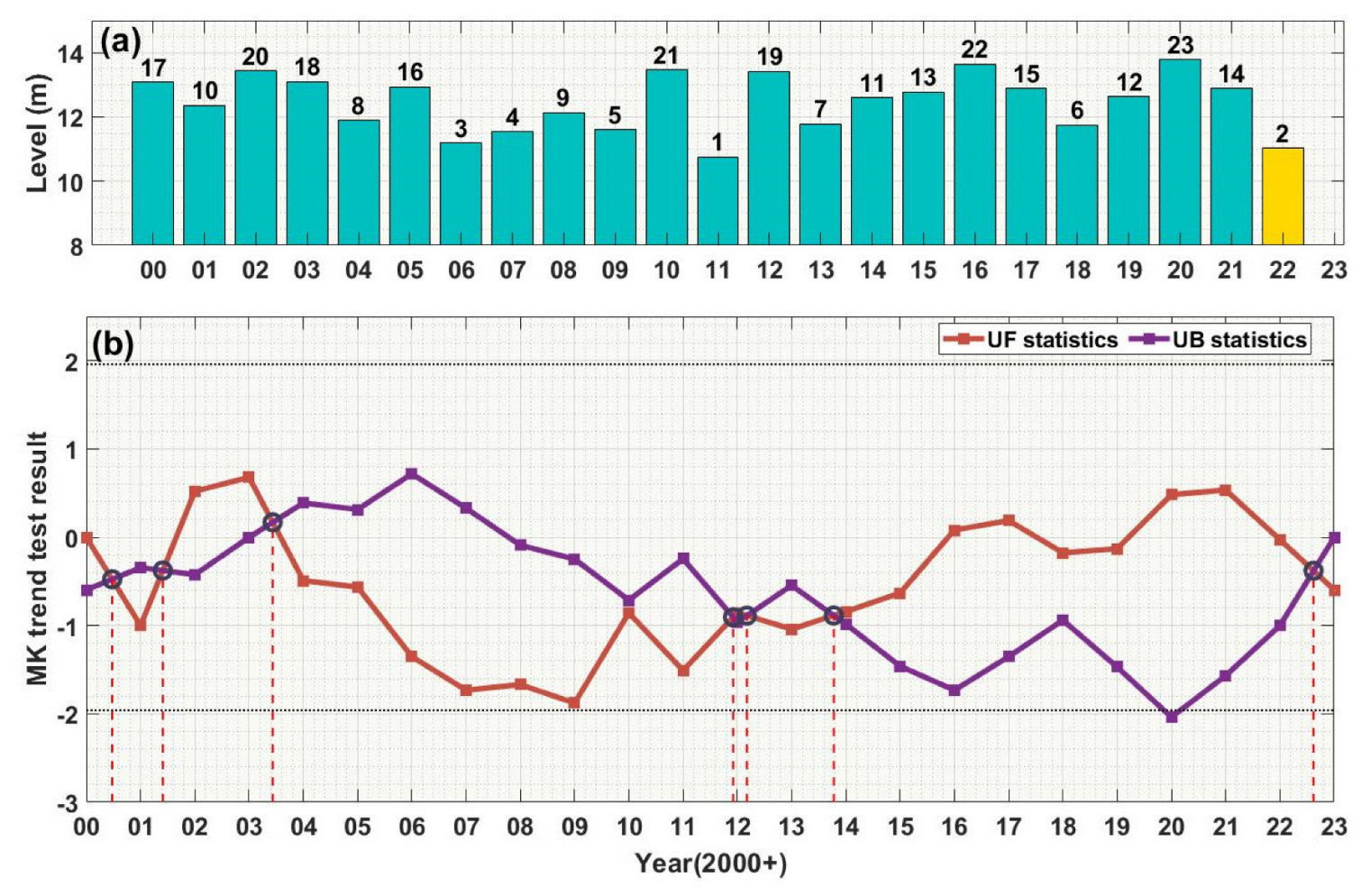
Long-term data indicated an extended period of abnormally low water levels, with a continuous decline from June to October 2022, reaching a minimum water level of only 6.4 m. Furthermore, the M-K trend test was utilized to capture a sudden change in water levels that occurred in July 2022.

(3)

The minimum lake area in nearly five years, obtained from SAR image data, occurred in 2022 with an area of only 814 km².

(4)

It was observed that there was a highly inadequate precipitation during the summer of 2022, with only 7.161 mm of rainfall in the PLB in September.

Furthermore, the vegetation index corresponded to the occurrence of extreme drought events, manifesting as a temporal lag of approximately one month compared to TWS variations, and in terms of spatial extent, it resulted in persistent water shortages that impacted vegetation growth across almost the entire PLB.

In conclusion, the characteristics of the extreme drought in the PLB in 2022 are the anomalous TWS observed by GRACE-FO and GLDAS, insufficient precipitation, extremely low water levels, and continuous widespread shrinkage of the lake area. The data show that the extreme drought event in the PLB in 2022 had a long duration, wide-ranging impacts, and high intensity.

Additionally, this study also identified a flood event in 2020, which to some extent demonstrates the suitability of the methods and analysis applied in this research to study flood events. Moreover, the methodology of this study provides a prior basis for establishing more accurate drought models in the PLB in subsequent studies.

References

1. Buitink, J.; van Hateren, T.C.; Teuling, A.J. Hydrological System Complexity Induces a Drought Frequency Paradox. Front. Water 2021, 3, 640976. [Google Scholar] [CrossRef]
2. Gampe, D.; Zscheischler, J.; Reichstein, M.; O’Sullivan, M.; Smith, W.K.; Sitch, S.; Buermann, W. Increasing impact of warm droughts on northern ecosystem productivity over recent decades. Nat. Clim. Chang. 2021, 11, 772–779. [Google Scholar] [CrossRef]
3. Jenkins, K.; Dobson, B.; Decker, C.; Hall, J.W. An Integrated Framework for Risk-Based Analysis of Economic Impacts of Drought and Water Scarcity in England and Wales. Water Resour. Res. 2021, 57, e2020WR027715. [Google Scholar] [CrossRef]
4. Feng, L.; Hu, C.; Chen, X.; Cai, X.; Tian, L.; Gan, W. Assessment of inundation changes of Poyang Lake using MODIS observations between 2000 and 2010. Remote Sens. Environ. 2012, 121, 80–92. [Google Scholar] [CrossRef]
5. Li, X.; Zhang, Q.; Zhang, D.; Ye, X. Investigation of the drought–flood abrupt alternation of streamflow in Poyang Lake catchment during the last 50 years. Hydrol. Res. 2016, 48, 1402–1417. [Google Scholar] [CrossRef]
6. Wei, W.; Zhang, J.; Zhou, L.; Xie, B.; Zhou, J.; Li, C. Comparative evaluation of drought indices for monitoring drought based on remote sensing data. Environ. Sci. Pollut. Res. 2021, 28, 20408–20425. [Google Scholar] [CrossRef]
7. Ma, Z.-C.; Sun, P.; Zhang, Q.; Hu, Y.-Q.; Jiang, W. Characterization and Evaluation of MODIS-Derived Crop Water Stress Index (CWSI) for Monitoring Drought from 2001 to 2017 over Inner Mongolia. Sustainability 2021, 13, 916. [Google Scholar] [CrossRef]
8. Wang, M.; Liu, T.; Ling, S.; Sui, X.; Yao, H.; Hou, X. Summary of Agricultural Drought Monitoring by Remote Sensing at Home and Abroad. In Proceedings of the Computer and Computing Technologies in Agriculture XI, Jilin, China, 12–15 August 2017; Springer: Cham, Switzerland, 2019; pp. 13–20. [Google Scholar]
9. Sun, P.; Ma, Z.; Zhang, Q.; Singh, V.P.; Xu, C.-Y. Modified drought severity index: Model improvement and its application in drought monitoring in China. J. Hydrol. 2022, 612, 128097. [Google Scholar] [CrossRef]
10. Chen, J.L.; Cazenave, A.; Dahle, C.; Llovel, W.; Panet, I.; Pfeffer, J.; Moreira, L. Applications and Challenges of GRACE and GRACE Follow-On Satellite Gravimetry. Surv. Geophys. 2022, 43, 305–345. [Google Scholar] [CrossRef]
11. Vishwakarma, B.D. Monitoring Droughts From GRACE. Front. Environ. Sci. 2020, 8, 584690. [Google Scholar] [CrossRef]
12. Cui, L.L.; Zhang, C.; Luo, Z.C.; Wang, X.L.; Li, Q.; Liu, L.L. Using the Local Drought Data and GRACE/GRACE-FO Data to Characterize the Drought Events in Mainland China from 2002 to 2020. Appl. Sci. 2021, 11, 9594. [Google Scholar] [CrossRef]
13. Xu, G.; Wu, Y.; Liu, S.; Cheng, S.; Zhang, Y.; Pan, Y.; Wang, L.; Dokuchits, E.Y.; Nkwazema, O.C. How 2022 extreme drought influences the spatiotemporal variations of terrestrial water storage in the Yangtze River Catchment: Insights from GRACE-based drought severity index and in-situ measurements. J. Hydrol. 2023, 626, 130245. [Google Scholar] [CrossRef]
14. Fok, H.S.; He, Q.; Chun, K.P.; Zhou, Z.; Chu, T. Application of ENSO and Drought Indices for Water Level Reconstruction and Prediction: A Case Study in the Lower Mekong River Estuary. Water 2018, 10, 58. [Google Scholar] [CrossRef]
15. Han, X.; Chen, X.; Feng, L. Four decades of winter wetland changes in Poyang Lake based on Landsat observations between 1973 and 2013. Remote Sens. Environ. 2015, 156, 426–437. [Google Scholar] [CrossRef]
16. Zeng, L.; Schmitt, M.; Li, L.; Zhu, X.X. Analysing changes of the Poyang Lake water area using Sentinel-1 synthetic aperture radar imagery. Int. J. Remote Sens. 2017, 38, 7041–7069. [Google Scholar] [CrossRef]
17. Zhang, Z.; Tian, J.; Huang, Y.; Chen, X.; Chen, S.; Duan, Z. Hydrologic Evaluation of TRMM and GPM IMERG Satellite-Based Precipitation in a Humid Basin of China. Remote Sens. 2019, 11, 431. [Google Scholar] [CrossRef]
18. Lu, J.; Jia, L.; Menenti, M.; Yan, Y.; Zheng, C.; Zhou, J. Performance of the Standardized Precipitation Index Based on the TMPA and CMORPH Precipitation Products for Drought Monitoring in China. IEEE J. Sel. Top. Appl. Earth Obs. Remote Sens. 2018, 11, 1387–1396. [Google Scholar] [CrossRef]
19. Li, Y.; Zhuang, J.; Bai, P.; Yu, W.; Zhao, L.; Huang, M.; Xing, Y. Evaluation of Three Long-Term Remotely Sensed Precipitation Estimates for Meteorological Drought Monitoring over China. Remote Sens. 2023, 15, 86. [Google Scholar] [CrossRef]
20. Lai, C.; Zhong, R.; Wang, Z.; Wu, X.; Chen, X.; Wang, P.; Lian, Y. Monitoring hydrological drought using long-term satellite-based precipitation data. Sci. Total Environ. 2019, 649, 1198–1208. [Google Scholar] [CrossRef]
21. Gomes, A.C.C.; Bernardo, N.; Alcântara, E. Accessing the southeastern Brazil 2014 drought severity on the vegetation health by satellite image. Nat. Hazards 2017, 89, 1401–1420. [Google Scholar] [CrossRef]
22. Zeng, J.; Zhang, R.; Qu, Y.; Bento, V.A.; Zhou, T.; Lin, Y.; Wu, X.; Qi, J.; Shui, W.; Wang, Q. Improving the drought monitoring capability of VHI at the global scale via ensemble indices for various vegetation types from 2001 to 2018. Weather Clim. Extrem. 2022, 35, 100412. [Google Scholar] [CrossRef]
23. Chao, N.; Wang, Z.; Jiang, W.; Chao, D. A quantitative approach for hydrological drought characterization in southwestern China using GRACE. Hydrogeol. J. 2016, 24, 893. [Google Scholar] [CrossRef]
24. Zhu, Y.; Liu, Y.; Wang, W.; Singh, V.P.; Ma, X.; Yu, Z. Three dimensional characterization of meteorological and hydrological droughts and their probabilistic links. J. Hydrol. 2019, 578, 124016. [Google Scholar] [CrossRef]
25. Ali, S.; Basit, A.; Ni, J.; Manzoor; Khan, F.U.; Sajid, M.; Umair, M.; Makanda, T.A. Impact assessment of drought monitoring events and vegetation dynamics based on multi-satellite remote sensing data over Pakistan. Environ. Sci. Pollut. Res. 2023, 30, 12223–12234. [Google Scholar] [CrossRef]
26. Agutu, N.; Awange, J.; Zerihun, A.; Ndehedehe, C.; Kuhn, M.; Fukuda, Y. Assessing multi-satellite remote sensing, reanalysis, and land surface models’ products in characterizing agricultural drought in East Africa. Remote Sens. Environ. 2017, 194, 287–302. [Google Scholar] [CrossRef]
27. Henchiri, M.; Liu, Q.; Essifi, B.; Javed, T.; Zhang, S.; Bai, Y.; Zhang, J. Spatio-temporal patterns of drought and impact on vegetation in North and West Africa based on multi-satellite data. Remote Sens. 2020, 12, 3869. [Google Scholar] [CrossRef]
28. Ran, Y.; Zhong, M.; Chen, W.; Zhong, Y.; Feng, W. Monitoring the extreme drought in the middle and lower reaches of the Yangtze River in 2019 from GRACE-FO satellites. Chin. Sci. Bull. 2021, 66, 107–117. [Google Scholar] [CrossRef]
29. Smakhtin, V.U.; Hughes, D.A. Automated estimation and analyses of meteorological drought characteristics from monthly rainfall data. Environ. Model. Softw. 2007, 22, 880–890. [Google Scholar] [CrossRef]
30. Tallaksen, L.M.; Hisdal, H.; Van Lanen, H.A. Space–time modelling of catchment scale drought characteristics. J. Hydrol. 2009, 375, 363–372. [Google Scholar] [CrossRef]
31. Ma, M.; Qu, Y.; Lyu, J.; Zhang, X.; Su, Z.; Gao, H.; Yang, X.; Chen, X.; Jiang, T.; Zhang, J.; et al. The 2022 extreme drought in the Yangtze River Basin: Characteristics, causes and response strategies. River 2022, 1, 162–171. [Google Scholar] [CrossRef]
32. Mishra, A.K.; Singh, V.P. Drought modeling—A review. J. Hydrol. 2011, 403, 157–175. [Google Scholar] [CrossRef]
33. West, H.; Quinn, N.; Horswell, M. Remote sensing for drought monitoring & impact assessment: Progress, past challenges and future opportunities. Remote Sens. Environ. 2019, 232, 111291. [Google Scholar] [CrossRef]
34. AghaKouchak, A.; Farahmand, A.; Melton, F.S.; Teixeira, J.; Anderson, M.C.; Wardlow, B.D.; Hain, C.R. Remote sensing of drought: Progress, challenges and opportunities. Rev. Geophys. 2015, 53, 452–480. [Google Scholar] [CrossRef]
35. Li, X.; Zhang, Q.; Ye, X. Capabilities of satellite-based precipitation to estimate the spatiotemporal variation of flood/drought class in Poyang Lake basin. Adv. Meteorol. 2013, 2013, 901240. [Google Scholar] [CrossRef]
36. Wu, G.; Liu, Y. Satellite-based detection of water surface variation in China’s largest freshwater lake in response to hydro-climatic drought. Int. J. Remote Sens. 2014, 35, 4544–4558. [Google Scholar] [CrossRef]
37. Zhang, D.; Chen, P.; Zhang, Q.; Li, X. Copula-based probability of concurrent hydrological drought in the Poyang lake-catchment-river system (China) from 1960 to 2013. J. Hydrol. 2017, 553, 773–784. [Google Scholar] [CrossRef]
38. Liu, Y.; Song, P.; Peng, J.; Fu, Q.; Dou, C. Recent increased frequency of drought events in Poyang Lake Basin, China: Climate change or anthropogenic effects. Hydro-Climatol. Var. Change 2011, 344, 99–104. [Google Scholar]
39. Zhang, Z.; Chen, X.; Xu, C.-Y.; Hong, Y.; Hardy, J.; Sun, Z. Examining the influence of river–lake interaction on the drought and water resources in the Poyang Lake basin. J. Hydrol. 2015, 522, 510–521. [Google Scholar] [CrossRef]
40. Sun, Y.; Riva, R.; Ditmar, P. Optimizing estimates of annual variations and trends in geocenter motion and J2 from a combination of GRACE data and geophysical models. J. Geophys. Res. Solid Earth 2016, 121, 8352–8370. [Google Scholar] [CrossRef]
41. Swenson, S.; Chambers, D.; Wahr, J. Estimating geocenter variations from a combination of GRACE and ocean model output. J. Geophys. Res. Solid Earth 2008, 113, B08410. [Google Scholar] [CrossRef]
42. Loomis, B.D.; Rachlin, K.E.; Luthcke, S.B. Improved Earth Oblateness Rate Reveals Increased Ice Sheet Losses and Mass-Driven Sea Level Rise. Geophys. Res. Lett. 2019, 46, 6910–6917. [Google Scholar] [CrossRef]
43. Loomis, B.D.; Rachlin, K.E.; Wiese, D.N.; Landerer, F.W.; Luthcke, S.B. Replacing GRACE/GRACE-FO with Satellite Laser Ranging: Impacts on Antarctic Ice Sheet Mass Change. Geophys. Res. Lett. 2020, 47, e2019GL085488. [Google Scholar] [CrossRef]
44. Swenson, S.; Wahr, J. Post-processing removal of correlated errors in GRACE data. Geophys. Res. Lett. 2006, 33, L08402. [Google Scholar] [CrossRef]
45. Duan, X.J.; Guo, J.Y.; Shum, C.K.; van der Wal, W. On the postprocessing removal of correlated errors in GRACE temporal gravity field solutions. J. Geod. 2009, 83, 1095–1106. [Google Scholar] [CrossRef]
46. Wu, Y.L.; Li, H.; Zou, Z.B.; Kang, K.X.; Liu, Z.W. Investigation of water storage variation in the Heihe River using the Forward-Modeling method. Chin. J. Geophys. Chin. Ed. 2015, 58, 3507–3516. [Google Scholar] [CrossRef]
47. Save, H.; Bettadpur, S.; Tapley, B.D. High-resolution CSR GRACE RL05 mascons. J. Geophys. Res. Solid Earth 2016, 121, 7547–7569. [Google Scholar] [CrossRef]
48. Save, H. CSR GRACE and GRACE-FO RL06 Mascon Solutions v02. 2020; [Data Set]; University of Texas: Austin, TX, USA, 2020; p. 10. [Google Scholar]
49. Beaudoing, H.; Rodell, M. GLDAS Noah Land Surface Model L4 Monthly 0.25 × 0.25 Degree V2.1; NASA: Greenbelt, MD, USA, 2020.
50. Schwatke, C.; Dettmering, D.; Bosch, W.; Seitz, F. DAHITI—An innovative approach for estimating water level time series over inland waters using multi-mission satellite altimetry. Hydrol. Earth Syst. Sci. 2015, 19, 4345–4364. [Google Scholar] [CrossRef]
51. Schwatke, C.; Scherer, D.; Dettmering, D. Automated extraction of consistent time-variable water surfaces of lakes and reservoirs based on landsat and sentinel-2. Remote Sens. 2019, 11, 1010. [Google Scholar] [CrossRef]
52. Yang, H.; Wang, H.; Lu, J.; Zhou, Z.; Feng, Q.; Wu, Y. Full Lifecycle Monitoring on Drought-Converted Catastrophic Flood Using Sentinel-1 SAR: A Case Study of Poyang Lake Region during Summer 2020. Remote Sens. 2021, 13, 3485. [Google Scholar] [CrossRef]
53. Li, Y.; Martinis, S.; Plank, S.; Ludwig, R. An automatic change detection approach for rapid flood mapping in Sentinel-1 SAR data. Int. J. Appl. Earth Obs. Geoinf. 2018, 73, 123–135. [Google Scholar] [CrossRef]
54. Didan, K. MOD13C2 MODIS/Terra Vegetation Indices Monthly L3 Global 0.05 Deg CMG V006; NASA EOSDIS Land Processes DAAC: Sioux Falls, SD, USA, 2015.
55. Huffman, G.; Stocker, E.; Bolvin, D.; Nelkin, E.; Tan, J. GPM IMERG Final Precipitation L3 1 Day 0.1 Degree × 0.1 Degree V06; Savtchenko, A., Greenbelt, M.D., Eds.; Goddard Earth Sciences Data and Information Services Center (GES DISC): Greenbelt, MD, USA, 2019. [CrossRef]
56. Muñoz-Sabater, J.; Dutra, E.; Agustí-Panareda, A.; Albergel, C.; Arduini, G.; Balsamo, G.; Boussetta, S.; Choulga, M.; Harrigan, S.; Hersbach, H. ERA5-Land: A state-of-the-art global reanalysis dataset for land applications. Earth Syst. Sci. Data 2021, 13, 4349–4383. [Google Scholar] [CrossRef]
57. Wahr, J.; Molenaar, M.; Bryan, F. Time variability of the Earth’s gravity field: Hydrological and oceanic effects and their possible detection using GRACE. J. Geophys. Res. Solid Earth 1998, 103, 30205–30229. [Google Scholar] [CrossRef]
58. Chambers, D.P. Evaluation of new GRACE time-variable gravity data over the ocean. Geophys. Res. Lett. 2006, 33, L17603. [Google Scholar] [CrossRef]
59. Chen, J.L.; Wilson, C.R.; Tapley, B.D.; Grand, S. GRACE detects coseismic and postseismic deformation from the Sumatra-Andaman earthquake. Geophys. Res. Lett. 2007, 34, L13302. [Google Scholar] [CrossRef]
60. Mann, H.B. Nonparametric tests against trend. Econom. J. Econom. Soc. 1945, 13, 245–259. [Google Scholar] [CrossRef]
61. Kendall, M.G. Rank Correlation Methods; Griffin: Stamford, CT, USA, 1948. [Google Scholar]
62. Hamed, K.H. Trend detection in hydrologic data: The Mann–Kendall trend test under the scaling hypothesis. J. Hydrol. 2008, 349, 350–363. [Google Scholar] [CrossRef]
63. Markert, K.N.; Chishtie, F.; Anderson, E.R.; Saah, D.; Griffin, R.E. On the merging of optical and SAR satellite imagery for surface water mapping applications. Results Phys. 2018, 9, 275–277. [Google Scholar] [CrossRef]
64. Hong, S.; Jang, H.; Kim, N.; Sohn, H.-G. Water Area Extraction Using RADARSAT SAR Imagery Combined with Landsat Imagery and Terrain Information. Sensors 2015, 15, 6652. [Google Scholar] [CrossRef]
65. Guo, Z.; Wu, L.; Huang, Y.; Guo, Z.; Zhao, J.; Li, N. Water-Body Segmentation for SAR Images: Past, Current, and Future. Remote Sens. 2022, 14, 1752. [Google Scholar] [CrossRef]
66. Tan, J.; Tang, Y.; Liu, B.; Zhao, G.; Mu, Y.; Sun, M.; Wang, B. A Self-Adaptive Thresholding Approach for Automatic Water Extraction Using Sentinel-1 SAR Imagery Based on OTSU Algorithm and Distance Block. Remote Sens. 2023, 15, 2690. [Google Scholar] [CrossRef]
67. Fensholt, R.; Rasmussen, K.; Nielsen, T.T.; Mbow, C. Evaluation of earth observation based long term vegetation trends—Intercomparing NDVI time series trend analysis consistency of Sahel from AVHRR GIMMS, Terra MODIS and SPOT VGT data. Remote Sens. Environ. 2009, 113, 1886–1898. [Google Scholar] [CrossRef]
68. Syed, T.H.; Famiglietti, J.S.; Rodell, M.; Chen, J.; Wilson, C.R. Analysis of terrestrial water storage changes from GRACE and GLDAS. Water Resour. Res. 2008, 44, W02433. [Google Scholar] [CrossRef]
69. Rodell, M.; Chen, J.; Kato, H.; Famiglietti, J.S.; Nigro, J.; Wilson, C.R. Estimating groundwater storage changes in the Mississippi River basin (USA) using GRACE. Hydrogeol. J. 2007, 15, 159–166. [Google Scholar] [CrossRef]
70. Wang, S.; Liu, H.; Yu, Y.; Zhao, W.; Yang, Q.; Liu, J. Evaluation of groundwater sustainability in the arid Hexi Corridor of Northwestern China, using GRACE, GLDAS and measured groundwater data products. Sci. Total Environ. 2020, 705, 135829. [Google Scholar] [CrossRef]
71. Yang, T.; Wang, C.; Yu, Z.; Xu, F. Characterization of spatio-temporal patterns for various GRACE- and GLDAS-born estimates for changes of global terrestrial water storage. Glob. Planet. Change 2013, 109, 30–37. [Google Scholar] [CrossRef]
72. Moghim, S. Assessment of Water Storage Changes Using GRACE and GLDAS. Water Resour. Manag. 2020, 34, 685–697. [Google Scholar] [CrossRef]
73. Wu, Q.; Si, B.; He, H.; Wu, P. Determining Regional-Scale Groundwater Recharge with GRACE and GLDAS. Remote Sens. 2019, 11, 154. [Google Scholar] [CrossRef]
74. Scanlon, B.R.; Zhang, Z.; Save, H.; Sun, A.Y.; Müller Schmied, H.; van Beek, L.P.H.; Wiese, D.N.; Wada, Y.; Long, D.; Reedy, R.C.; et al. Global models underestimate large decadal declining and rising water storage trends relative to GRACE satellite data. Proc. Natl. Acad. Sci. USA 2018, 115, E1080–E1089. [Google Scholar] [CrossRef]
75. Yuan, Y.; Zeng, G.; Liang, J.; Huang, L.; Hua, S.; Li, F.; Zhu, Y.; Wu, H.; Liu, J.; He, X. Variation of water level in Dongting Lake over a 50-year period: Implications for the impacts of anthropogenic and climatic factors. J. Hydrol. 2015, 525, 450–456. [Google Scholar] [CrossRef]
76. Leira, M.; Cantonati, M. Effects of water-level fluctuations on lakes: An annotated bibliography. In Ecological Effects of Water-Level Fluctuations in Lakes; Springer: Dordrecht, The Netherlands, 2008; pp. 171–184. [Google Scholar]
77. Wu, H.; Li, J.; Song, F.; Zhang, Y.; Zhang, H.; Zhang, C.; He, B. Spatial and temporal patterns of stable water isotopes along the Yangtze River during two drought years. Hydrol. Process. 2018, 32, 4–16. [Google Scholar] [CrossRef]
78. Wang, R.; Peng, W.; Liu, X.; Wu, W.; Chen, X.; Zhang, S. Responses of Water Level in China’s Largest Freshwater Lake to the Meteorological Drought Index (SPEI) in the Past Five Decades. Water 2018, 10, 137. [Google Scholar] [CrossRef]
79. Feng, L.; Hu, C.; Chen, X. Satellites Capture the Drought Severity Around China’s Largest Freshwater Lake. IEEE J. Sel. Top. Appl. Earth Obs. Remote Sens. 2012, 5, 1266–1271. [Google Scholar] [CrossRef]
80. Xing, Z.; Yu, Z.; Wei, J.; Zhang, X.; Ma, M.; Yi, P.; Ju, Q.; Wang, J.; Laux, P.; Kunstmann, H. Lagged influence of ENSO regimes on droughts over the Poyang Lake basin, China. Atmos. Res. 2022, 275, 106218. [Google Scholar] [CrossRef]
Figure 1. Location of the study area and concerned hydrological stations ((a) the location of the Yangtze River basin; (b) the location of the PLB).
Remotesensing 15 05125 g001
Figure 2. Comparison of spatial distribution of TWS variations in the PLB for July 2021 using different datasets. (af) represent the spatial distribution results of TWS variations obtained from the CSR spherical harmonic coefficient dataset, GFZ spherical harmonic coefficient dataset, JPL spherical harmonic coefficient dataset, CSR Mascon dataset, CSR spherical harmonic coefficient dataset with leakage correction, and GLDAS hydrological model calculations, respectively. (The resolution of all six images is consistent, and different color bars have been set for each).
Remotesensing 15 05125 g002
Figure 3. Comparison of TWS variations sequences obtained from different datasets (the labels from left to right, respectively, represent the time series of TWS changes obtained by the CSR Mascon dataset, CSR spherical harmonic coefficient dataset with leakage correction, GLDAS hydrological model, and CSR spherical harmonic coefficient dataset) in PLB from June 2018 to December 2022.
Remotesensing 15 05125 g003
Figure 4. Comparison of TWS variations sequences obtained from different datasets (the labels from left to right, respectively, represent the CSR Mascon dataset, CSR spherical harmonic coefficient dataset with leakage correction, GLDAS hydrological model, and CSR spherical harmonic coefficient dataset) in PLB from June 2018 to December 2022 (non−seasonal).
Remotesensing 15 05125 g004
Figure 5. (ai) represent the monthly average water level statistical information (including maximum, minimum, and mean values) of Hukou Station obtained from on-site observations during the period from 2014 to 2022, respectively.
Remotesensing 15 05125 g005
Figure 6. Comparison of the water levels for the same period. (a) Daily variations in water levels for the years 2016, 2018, 2019, 2020, and 2022; (b) monthly average water levels for the year 2022 represented by yellow bars, and monthly average water levels from 2000 to 2023 represented by blue bars.
Remotesensing 15 05125 g006
Figure 7. The average annual water level changes at Hukou Station from 2000 to 2022 were analyzed. (a) Rankings of the average annual water levels from 2000 to 2023 are displayed above the bars; (b) The trend analysis of the annual average water levels from 2000 to 2022 was conducted using the M−K test. The resulting plot includes the orange-red line representing the UF statistic, the purple line representing the UK statistic, and the black dashed lines representing the critical lines at the significance level of α = 0.05 (statistical values of ±1.96).
Remotesensing 15 05125 g007
Figure 8. The comparison of terrestrial water storage anomalies (TWSAs) in the PLB includes data obtained from the GRACE gravity field model covering from June 2018 to December 2022 (blue line), water levels derived from the DAHITI dataset spanning from 27 January 2018 to 25 May 2023 (orange line), and observed water level data from the Hukou station encompassing from 1 January 2018 to 13 July 2023 (purple line). The data period is restricted from January 2018 to July 2023. The inconsistent data spans and sampling intervals are due to variations in data availability.
Remotesensing 15 05125 g008
Figure 9. The SAR area from 2018 to 2021, the DAHITI area from 2018 to 2021, and the residuals between them.
Remotesensing 15 05125 g009
Figure 10. The monthly time series data of Poyang Lake area assessed by SAR images and the monthly time series data of TWSA in the PLB obtained from the GRACE gravity field model from 2018 to 2023.
Remotesensing 15 05125 g010
Figure 11. The water bodies of Poyang Lake extracted from SAR image data in early August from 2015 to 2022. (ah) The dark green areas represent the water body regions extracted for each year, while the orange-red area represents the water body of Poyang Lake in early August 2022 used for comparison.
Remotesensing 15 05125 g011
Figure 12. Difference in vegetation normalization index between 2018 and 2022 (subtract the data from 2022 at the same time period from the data of the past 18 years). (ah) represents the differences for the months from June to December and the following January of the next year.
Remotesensing 15 05125 g012
Figure 13. The monthly time series data of precipitation in the PLB from 2018 to 2022 and the monthly time series data of TWSA in the PLB obtained from the GRACE gravity field model.
Remotesensing 15 05125 g013
Figure 14. The difference of precipitation and evapotranspiration in PLB from 2018 to 2022. “Deviation” represents the difference between precipitation and evapotranspiration (purple line), while the red bars and blue bars represent precipitation and evaporation, respectively. The precipitation and evapotranspiration data are sourced from the ERA5 reanalysis dataset. The yellow coordinate axis lines represent the range of the purple line.
Remotesensing 15 05125 g014
Figure 15. The relationship between the area and water level of Poyang Lake. (a,b) represent the linear and quadratic fitting results of DAHITI water level and DAHITI area from June 2002 to February 2021. (c,d) represent the linear and cubic fitting results of measured water level data from Hukou station and SAR area from January 2018 to June 2023. (e,f) represent the linear and cubic fitting results of measured water level data from Hukou station and DAHITI area from June 2002 to February 2021. The left column displays the results of linear fitting, while the right column displays the results of non−linear fitting (we conducted quadratic and cubic non−linear fitting, retaining the best non-linear fitting result). The inconsistent data spans and sampling intervals are due to variations in data availability.
Remotesensing 15 05125 g015