A Siamese Multiscale Attention Decoding Network for Building Change Detection on High-Resolution Remote Sensing Images

Abstract

The objective of building change detection (BCD) is to discern alterations in building surfaces using bitemporal images. The superior performance and robustness of various contemporary models suggest that rapid development of BCD in the deep learning age is being witnessed. However, challenges abound, particularly due to the diverse nature of targets in urban settings, intricate city backgrounds, and the presence of obstructions, such as trees and shadows, when using very high-resolution (VHR) remote sensing images. To overcome the shortcomings of information loss and lack of feature extraction ability, this paper introduces a Siamese Multiscale Attention Decoding Network (SMADNet). This network employs the Multiscale Context Feature Fusion Module (MCFFM) to amalgamate contextual information drawn from multiscale target, weakening the heterogeneity between raw image features and difference features. Additionally, our method integrates a Dual Contextual Attention Decoding Module (CADM) to identify spatial and channel relations amongst features. For enhanced accuracy, a Deep Supervision (DS) strategy is deployed to enhance the ability to extract more features for middle layers. Comprehensive experiments on three benchmark datasets, i.e., GDSCD, LEVIR-CD, and HRCUS-CD, establish the superiority of SMADNet over seven other state-of-the-art (SOTA) algorithms.

1. Introduction

Change detection (CD) in remote sensing imagery aims to identify and extract variations from multitemporal images captured over an identical surface area [1]. This technique plays an important role in diverse applications, including urban planning [2], land use analysis [3], agricultural monitoring [4], and disaster evaluation [5]. Advancements in satellite technology have facilitated the acquisition of very high-resolution (VHR) remote sensing images, characterized by their expansive coverage, superior spectral resolution, and multisource attributes [6,7]. These VHR images enable the extraction of enhanced spatial and shape features, prompting an increasing number of researchers to adopt them for more refined and detailed CD endeavors [8]. As urbanization accelerates, building change detection (BCD) catches the eye, specifically in illegal urban building identification [9].

Conventional binary CD differentiates between changed and unchanged regions within bitemporal images [10]. The traditional BCD methods can be bifurcated based on research objectives: pixel-based techniques and object-based methodologies [11]. Pixel-based BCD is the simplest method, which takes independent image elements as detection units, extracts change information by analyzing image element spectral differences through pixel-by-pixel operations, and obtains the final change map through threshold segmentation. Despite its straightforward implementation, this method often overlooks crucial spatial context. As VHR remote sensing imagery evolves, there is a palpable shift from rudimentary pixel-based analysis to the more sophisticated object-based analysis. The research that uses these methods mainly aims at targets with more obvious features, such as buildings. Object-based methods segment remote sensing images into distinct entities, harnessing the abundant spectral, textural, structural, and geometric data within the imagery to detect variations on temporal images [12,13,14,15,16]. Nevertheless, extracting traditional manual features remains challenging, even when capitalizing on the spatial context available in VHR images [17].

In recent years, deep learning has made remarkable strides in image analysis and natural language processing domains [18,19], extending its influence to the realm of remote sensing image interpretation [20]. The Convolutional Neural Network (CNN), as a powerful deep learning structure, can extract abundant features from remote sensing images and is widely used in remote sensing image BCD tasks [21]. A variety of CD methodologies rooted in deep learning paradigms have emerged [22,23,24]. Long et al. [25] proposed a fully convolutional network (FCN) consisting of an encoder–decoder structure, whose encoder is similar to the traditional CNN, but it can accept the input of arbitrary size, and the decoder recovers the extracted features into a prediction map of the same size as the input image, preserving the original spatial information and finally achieving pixel-by-pixel prediction. Based on FCN, Ronneberger et al. [26] proposed Unet with a symmetric U-shaped encoder–decoder structure to fuse depth features in a top-to-bottom manner to improve accuracy. Most deep learning algorithms for CD are based on CNNs and FCNs [27,28,29]. Daudt et al. [30] proposed three different full convolutional neural network structures: FC-early fusion (FC-EF), FC-Siam-conc and FC-Siam-diff. While FC-EF is an early fusion method, the latter two both adopt the concept of jump connection in Unet, whose difference only lies in how to implement the jump connection.

However, it is prone to ignore the information in raw images when the network is too deep. PSPNet [31] proposed a pyramid network with different downsampling steps to obtain different perceptual fields that can capture information at different scales. DeepLabv3+ [32] proposed a dilation convolution with different dilation rates to design an atrous spatial pyramid pooling (ASPP) module to obtain multiscale information while maintaining a high-resolution feature map. ChangeNet [33] is a Siamese network where the weights of the upper and lower CNNs are shared, and upsampling uses bilinear interpolation instead of convolution. The outputs of the two parallel networks are then concatenated to improve performance. CDNet [34] is a two-stage cross-modal fusion scheme that combines fused depth features with RGB features to generate prediction maps. Zhou et al. [35] improved the Unet structure by adding hopping layer connections with additional multiscale feature layers and the new network was named Unet++, which integrates both long-connected and short-connected structure. Peng et al. [36] superimposed the aligned image pairs and then it was fed into a modified Unet++ network to generate change result maps in an end-to-end manner. It was named Unet++ MSOF, which has an excellent multiscale fusion ability and greatly improves the performance of detection. CLNet [37] uses Unet as the backbone and embeds a newly designed cross-layer block to fuse multiscale features and multilayer contextual information. DSAMNet [38] integrates convolutional block attention module (CBAM) and deeply supervised (DS) module, which provides more discriminative features. DASNet [39] uses channel and spatial attention to establish connections between local features, which is used to obtain global contextual information to better distinguish between areas that have changed and those that have not. The Transformer [40] is a network architecture that relies only on the attention mechanism and is gradually used in various fields. In BCD tasks, Transformer is introduced to model the contextual content of bitemporal images, which facilitates the identification of real changes in the image and excludes irrelevant changes. ChangeFormer [41] is a Transformer-based Siamese network architecture for CD from a pair of remote sensing images, which can effectively present multiscale remote details. STCD [42] is a Siamese transformer-based network using pure transformers without CNN to model the long-range context of semantic tokens, but the ability to reduce computational overhead is weak. These methods integrate feature extraction and difference discrimination operations, and the results are generated via an end-to-end manner, thereby minimizing error transmission. Despite the above efforts, challenges still exist in the BCD task.

Existing frameworks for CD can be classified into three categories: single-stream framework, dual-stream framework, and multimodel integration framework [43]. The single-stream framework predominantly utilizes direct classification methodologies, with data fusion being its cornerstone [44]. Given that CD tasks customarily employ dual-temporal imagery as inputs, the dual-stream framework emerges as a preferred choice for many researchers, which is mainly classified into three types: twin structure, migration learning-based structure, and post-classification structure. The twin structure usually consists of two subnets with the same structure, which share with weights to extract features. The main advantage of this structure is that the two subnets are trained directly and learn the features of the input dual-time image data simultaneously, which enables the feature extractor to learn the depth features directly by supervised training with labeled samples [28,33]. The multimodel integration framework is similar to the dual-stream structure but contains more models, which makes the whole process of CD more complex when trying to improve performance [45].

However, most FCNs in CD studies are modified from single-stream semantic segmentation networks. Concatenating bitemporal images as one input makes the early layers of the network unable to extract informative features of raw images. In addition, notable information loss occurs due to the repeated usage of pooling layers used for image downsampling, thus affecting accuracy. Furthermore, an excessively deep architecture may cause gradient vanishing, slow convergence, and overfitting. In addition, the diverse nature of targets in urban settings, intricate city backgrounds, and the presence of obstructions such as trees and shadows pose great challenges in BCD on VHR remote sensing images.

To solve above problems, we propose a Siamese multiscale attention decoding network (SMADNet) for bitemporal image BCD. First, multiscale features from different levels of input bitemporal images are extracted by means of a Siamese feature encoder, then the extracted features are fused using the multiscale context feature fusion module (MCFFM). Subsequently, The Dual Contextual Parsing Module (DCPM) is deployed to enrich the MCFFM-derived features with both channel and spatial attention, thereby minimizing information loss. To combat issues like gradient vanishing, a Deep Supervision (DS) strategy is seamlessly integrated into the network, amplifying the efficacy of the disparity map recognition network. Finally, the cumulative outputs of these modules are unified under a hybrid loss function, facilitating effective network training. In addition, recognizing the inherent dependency of deep learning models on extensive data samples and catering to diverse change detection scenarios, we validate our approach on three widely recognized datasets: GDSCD [46], LEVIR-CD [47] and HRCUS-CD [48].

The main contributions of this paper are as follows:

(1)

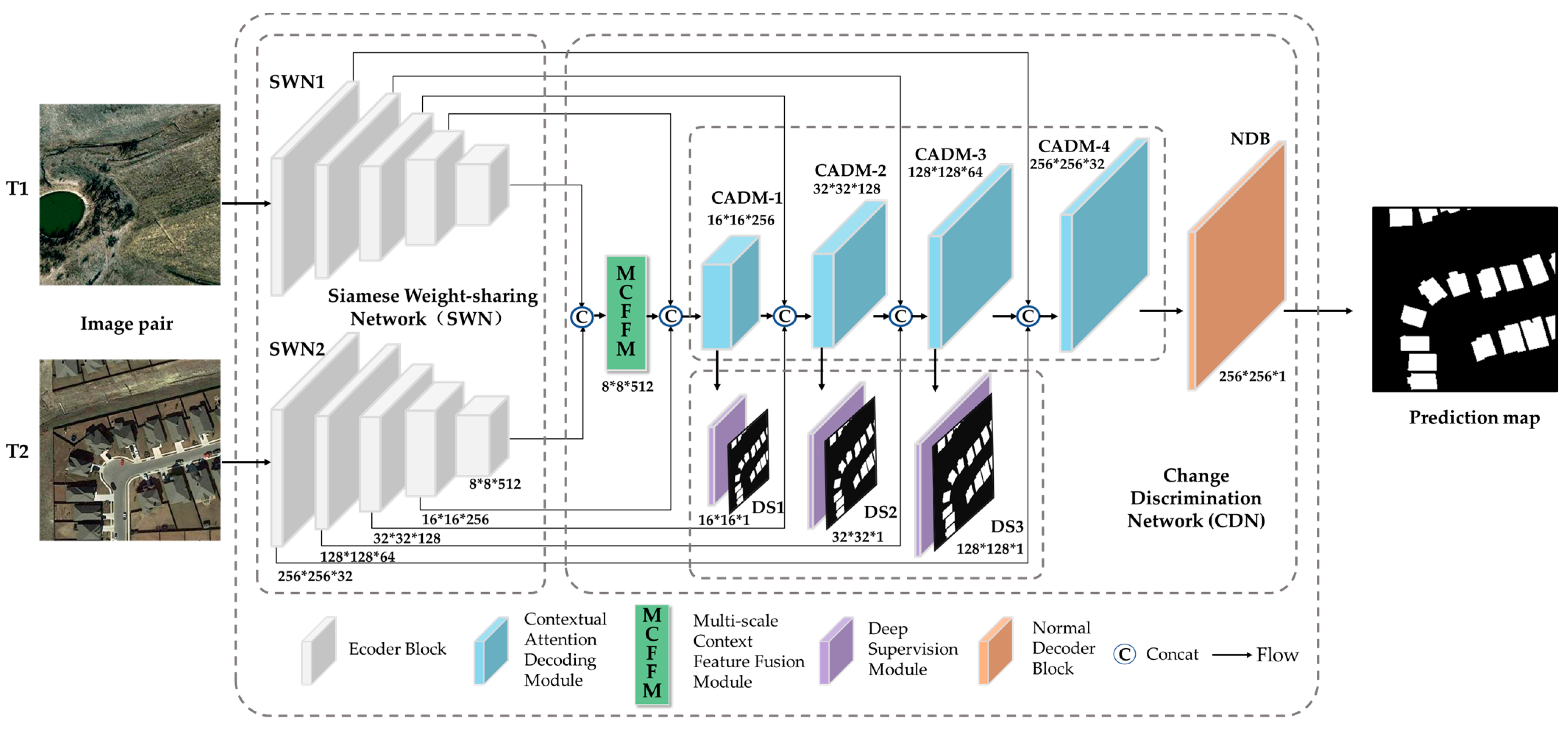
We introduce SMADNet, employing the Multiscale Context Feature Fusion Module (MCFFM) and integrating the Dual Contextual Attention Decoding Module (CADM). In addition, it incorporates the Deep Supervision (DS) strategy in the middle layers of the decoder to assist in training network parameters, thus improving the generalization ability and detection accuracy.

(2)

We propose a novel Dual Contextual Attention Decoding Module (CADM). The combination of a parallel structure and CADM can effectively suppress pseudo-changes and leads to better integration of raw image feature and difference features, achieving information retention.

(3)

We perform rigorous experiments using widely recognized change detection datasets, further buttressed by comprehensive ablation studies. The subsequent qualitative and quantitative evaluations reinforce the proposed method’s preeminence, underscoring its potential for building change detection applications.

The rest of the paper is organized as follows. Section 2 describes the proposed SMADNet network in detail. The experimental procedure and ablation experiments are described in detail and the experimental results. The results of comparison experiments and ablation experiments are given in Section 3. Some additional discussions of the experimental results are shown in Section 4. Finally, the research is concluded in Section 5.

2. Methods

In this section, we describe the proposed network in detail. First, the overall structure of SMADNet is introduced. Subsequently, three important components of the network, MCFFM, CADM, and DS strategy, are explained in detail, subsequently. The hybrid loss function used is then introduced.

2.1. Overview

The network structure proposed in this section is shown in Figure 1. SMADNet is an end-to-end network, which consists of two main components: the Siamese weight-sharing network (SWN) and the change discrimination network (CDN).

SWN aims at transform bitemporal images into a consistent feature space while preserving the distinct features of each image, which use a Siamese weight-sharing network to finish feature extraction as the encoder. The backbone of the SWM is the architecture of the pretrained ResNet34 [49] before the global average pooling layer. In addition, CDN is a decoder of proposed network, which is mainly composed of MCFFM and CADM.

First, prechange image T1 and postchange image T2, bitemporal images, are used as separate inputs to two parallel streams, SWN1 and SWN2, preserving the original features of each individual image as much as possible. Then, the encoder with the shared structure and parameters is applied to streams for feature extraction of the original image. After progressive abstraction of the convolution and pooling layers, the extracted deep features from the two parallel streams are joined and aggregated into one stream, which enters MCFFM for feature fusion, followed by CADM step for feature decoding and disparity recognition. Finally, a common decoding block outputs a single-channel binary prediction label.

There are five stages of every SWN1 and SWN2 connected with CADM. The early layers in the SWN, i.e., Stage1–Stage4, contain lower-level local structure information of the dual-temporal image, and they are connected to the CADM with the same scale by skip connections that complement the features of individual temporal images and also provide both high- and low-level instinct features to the subsequent modules. After convolutional and pooling layers, the deepest layers in streams T1 and T2 acquire large perceptual fields and compact rich contextual information, so that Stage5 of the two parallel streams from SWN are connected in the channel dimension and act as initial input to the MCFFM in which the multiscale feature fusion process is performed. Then the connection between the features is established using the dual attention mechanism. The features fused by the MCFFM and Stage4 from SWN are concatenated in the channel dimension and input to CADM-1 to generate an initial global change map with compact dimensions. The outputs of CADM-4 are used as the input of the last normal decoding block (NDB). In the standard decoding block, no attention mechanisms have been incorporated. The block comprises a conventional convolution module, a 1 × 1 convolution layer, and a sigmoid function dedicated to producing the final change map. Supervision extends beyond just the output layer of the backbone network. To aid in training and boost the network’s generalization capability, three Deep Supervision layers (DS1, DS2, and DS3), all possessing identical structures, are integrated to generate corresponding change maps.

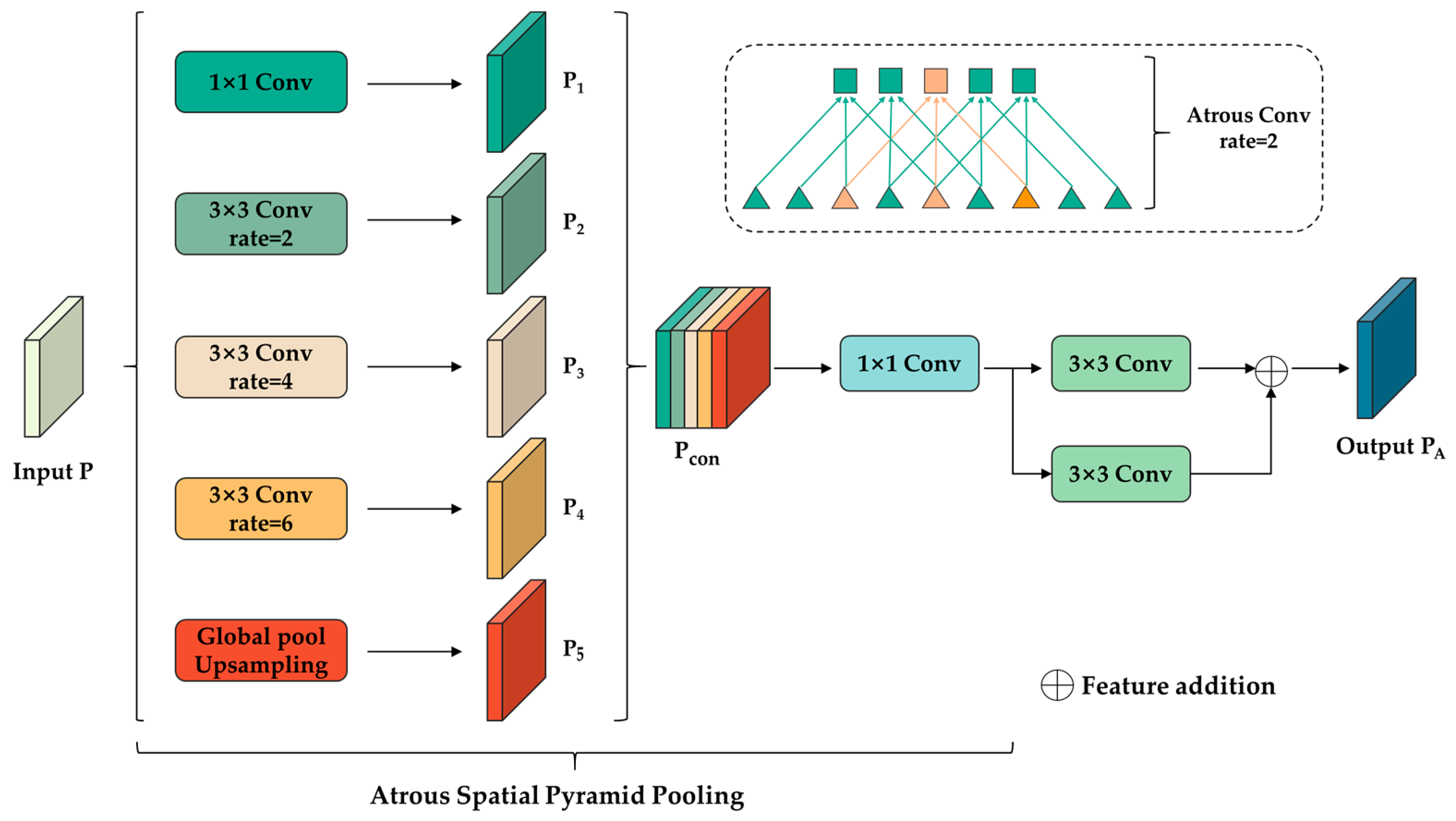
2.2. Multiscale Context Feature Fusion Module

In the proposed network, we use the MCFFM for the process of multiscale feature fusion (see Figure 2). The MCFFM mainly consists of atrous spatial pyramid pooling (ASPP) and two ordinary convolutional layers.

The ASPP module consists of five parallel branches. The first branch contains a 1 × 1 convolutional layer, and the second, third, and fourth branches contain a 3 × 3 atrous convolutional layer with dilation rates of 2, 4 and 6, respectively. The fifth branch contains a global pooling layer and an upsampling operation to integrate the global information. The original features P are extracted into five different branches to features P₁, P₂, P₃, P₄ and P₅, which have the same size. The fused feature P_con is obtained by cascading five features through the channels. Then P_con is fed into a 1 × 1 convolution to adjust the number of channels, and then a 1 × 1 convolution and a 3 × 3 convolution with residual concatenation are used for further feature extraction.

The convolution in ASPP is atrous convolution, and the kernel size is always kept constant at 3 × 3, which can expand the perceptual field without losing resolution. Using ASPP in semantic segmentation to combine semantic information of different receptive fields can achieve free multiscale feature extraction and improve segmentation accuracy.

The pooling layer in ASPP is a two-dimensional adaptive mean pooling layer. The so-called adaptive mean pooling means that it is not necessary to specify the kernel size and step, but only the final output size (1 × 1 here). The features of each channel are extracted by compressing the feature maps of each channel separately to 1 × 1, and, thus, the global features are obtained. Then a 1 × 1 convolution layer is used to further extract the features obtained in the previous step and reduce the dimensionality.

The computation process of ASPP is as follows:

$$P_{\mathit{aspp}}={f }^{1\times 1}\left(\left[ f^{1\times 1}\left(P\right);{ f }_{r=2}^{3\times 3}\left(P\right);{ f }_{r=4}^{3\times 3}\left(P\right);{ f }_{r=6}^{3\times 3}\left(P\right); \mathit{up}\left(\mathit{glo} \mathit{pool}\left(P\right)\right)\right]\right)$$

(1)

where $P$ denotes the input feature, $f^{1\times 1}$ denotes the 1 × 1 convolution operation, $f_{r=2}^{3\times 3}$, ${ f }_{r=4}^{3\times 3}$, and ${f }_{r=6}^{3\times 3}$ denote the atrous convolution operation with a null rate of 2, 4 and 6, respectively; $up$ denotes the upsampling operation; $\mathit{glo} \mathit{pool}$ denotes the global average pooling; and $[;]$ denotes the feature cascade.

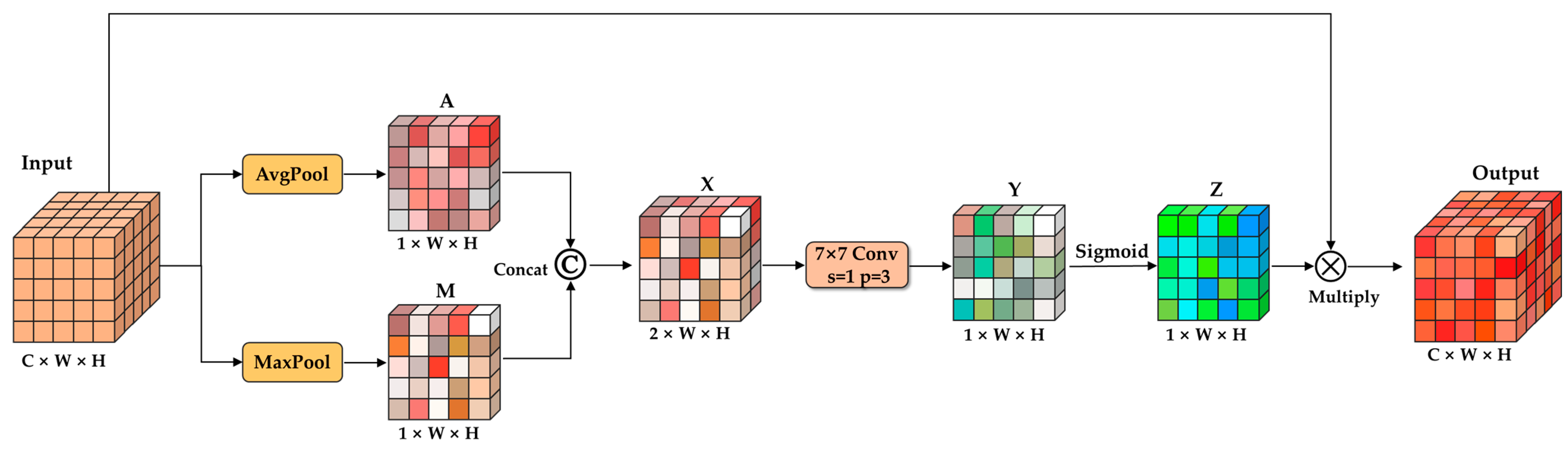
2.3. Contextual Attention Decoding Module

The architecture of the CD model predominantly comprises an encoder and a decoder. The encoder’s role is to represent the input, while the decoder is tasked with generating the output. To formulate the CADM, we employ both the SAM and the CAM, and these are synergized with transpose convolution (DeConv). The CADM forms the primary structure of the CDN, spanning from CADM-1 to CADM-4. Additionally, the CDN encompasses two distinct blocks: the CADM and the NDB, which are presented in Figure 3 and Figure 4, respectively.

Within CADM, the operational sequence begins with the input features being processed by the CAM. This mechanism assigns weights to each channel to produce a weighted feature representation. These weighted features are then enhanced by integrating with residual connections. Subsequent to this integration, a 3 × 3 convolution is applied to facilitate feature fusion, followed by a 1 × 1 convolution aimed at channel compression. Upon compression, these features are channeled into the SAM for the generation of spatial attention features. To further enhance these features and circumvent the gradient disappearance issue, they are merged with residual connections. The features then undergo two sequential 3 × 3 convolutions to accentuate the change attributes. The resultant feature map is simultaneously dispatched to the DS layer for advanced processing and to the DeConv for upsampling, ensuring a refined granularity of the feature map. This comprehensive process captures the entirety of CADM’s functionality, delivering meticulous feature processing and enrichment.

After four CADMs, the resolution of the feature map is restored to the original resolution. At this time, the features are further extracted and the channels are compressed using the common decoding blocks, and finally, the probability map of each pixel point change is obtained via the Sigmoid function. Then the predicted binary labels are generated by threshold segmentation.

Addressing the heterogeneity issue arising from the amalgamation of features across diverse domains is crucial. To this end, we have incorporated an attention block designed to adeptly merge features emanating from these different domains. The essence of channel attention lies in its ability to formulate a channel attention feature map by leveraging the interrelationships among feature channels. This can be conceptualized as a process of allocating channel-specific weights, providing greater emphasis to channels rich in pertinent information and diminishing the emphasis on less significant channels. By multiplying the computed channel attention feature vector with every channel of the input image, a feature map enriched with channel attention is generated. A visual representation detailing the mechanics of the channel attention mechanism is delineated in Figure 5.

The computation process of channel attention is as follows:

$$F_{\mathit{ca}}=F \times \left(\mathit{\sigma }\left(\mathit{MLP}\left(\mathit{AvgPool} \left(F\right)\right)\right)+\mathit{MLP}\left(\mathit{MaxPool} \left(F\right)\right)\right)$$

(2)

where $F$ denotes the input feature map, $\mathit{\sigma }$ denotes the Sigmoid function. First, the spatial information of the input feature map is compressed by the average pooling (AvgPool) operation and the maximum pooling (MaxPool) operation along the spatial axis. Suppose there are C feature maps of size H × W. After the pooling operation, the feature maps will be squeezed into two vectors of size C × 1 × 1. Then, each vector is forwarded to a shared multilayer perceptron (MLP). The output of the shared MLP is merged by using element-by-element summation. Then, a Sigmoid function is appended to assign weights to each channel. Finally, the input features $F$ are multiplied by S to obtain the output features $F_{ca}$.

The inclusion of the spatial attention mechanism serves a pivotal role: it assigns varying weights across distinct spatial locations on the feature map, highlighting the differential significance each spatial location holds in the feature extraction process. Within the spatial attention module, connections between any two positions on the feature map are established via the attention mechanism. This ensures that the feature information from every location on the map is captured through a weighted summation corresponding to a specific location. Enhancing the network model’s feature representation capability is achieved by aggregating these input features with their respective spatial location feature components. Through the spatial attention mechanism, the weightage for critical spatial locations is accentuated, thereby rendering these crucial features more potent. An added advantage is that this elevation in potency does not significantly augment computational demands, ensuring the computational speed of the network model remains largely unaffected. A comprehensive depiction of the spatial attention mechanism can be found in Figure 6.

First, the input features T are passed through a maximum pooling operation and an average pooling operation along the channel axis to obtain the features T_max and T_avg. Further, T_max and T_avg are cascaded along the channel and passed into a 7 × 7 convolution layer to obtain the initial weight matrix G. Then, the Sigmoid function is used to obtain the final weight matrix G_s. Finally, the input features T are multiplied by the weight matrix G_s to obtain output features $T_{sa}$:

$$T_{\mathit{sa}}=T \times \left(\mathit{\sigma }\left({f }^{7\times 7}\left(\left[\mathit{MaxPool}\left(T\right); \mathit{AvgPool}\left(T\right)\right]\right)\right)\right)$$

(3)

where $\mathit{\sigma }$ denotes the Sigmoid function, ${f }^{7\times 7}$ denotes the 7 × 7 convolution operation, and $[;]$ denotes the feature cascade.

Finally, we input $T_{\mathit{sa}}$ into two 3 × 3 convolutions to extract the change features, and finally pass the feature map to the transposed convolution module, in which the upsampling operation is performed to obtain the result ${\mathit{CADM}}_i$:

$${\mathit{CADM}}_i={f }_{\mathit{DeCon}}^{2\times 2}\left({ f }^{3\times 3}\left({f }^{3\times 3}\left(T_{\mathit{sa}}\right)\right)\right)$$

(4)

where ${f }_{\mathit{DeCon}}^{2\times 2}$ denotes the 2 × 2 transposed convolution, ${ f }^{3\times 3}$ denotes the 3 × 3 convolution operation.

2.4. Deep Supervision

To alleviate the gradient disappearance problem and improve the performance of SMADNet, we introduce the DS layer to effectively train the network. Not only relying on the backpropagation of gradients in the output layer, the intermediate layers are also supervised by change maps with different spatial resolutions. By receiving direct feedback from the change maps, the features generated by the intermediate layer have better results for the identification of change regions. Finally, the model is expected to approach the change region more rapidly. Specifically, for each spatially refined set of image difference features in CDN, we associate them with the same scale of downsampled change maps. The three branches of the DS module are denoted as DS₁, DS₂ and DS₃. The DS auxiliary branch ${DS}_i$ is computed as follows:

$${\mathit{DS}}_i=\mathit{\sigma }\left({f }^{1\times 1}\left(T_i\right)\right)$$

(5)

where $T_i$ denotes the feature branch of the ${\mathit{CADM}}_i$ that flows into the DS module. σ represents the sigmoid function and ${f }^{1\times 1}$ represents the 1 × 1 convolution operation. During the training process, the loss of each depth supervision is computed independently and backpropagated directly to the intermediate layers. In this way, the intermediate layers in the network are trained efficiently and the weights of the intermediate layers can be finely updated, thus alleviating the problem of gradient disappearance. Thus, when the previous layers have been finely trained for initial change detection, the following layers will face a simple change detection task. By introducing multiple deep supervision in the network, the performance of the difference recognition network is improved.

2.5. Loss Function

For binary change images, Binary Cross Entropy (BCE) loss function is used with the purpose of classifying building information into two categories: changed and unchanged.

$$L_{\mathit{bce} }= -\frac{1}{m\times n_0}\sum _{i=1}^m\sum _{j=1}^n\left[y_{\left(i,j\right)}\mathit{log}\left(p_{\left(i,j\right)}\right)+\left(1-y_{\left(i,j\right)}\right)\mathit{log}\left(1 - p_{\left(i,j\right)}\right)\right]$$

(6)

where $y_{\left(i,j\right)}$ represents the true value of pixel j in the ground truth map in layer i after one encoding. $y_{\left(1,j\right)}$ = 0 and $y_{\left(2,j\right)}$ = 1 indicates that pixel j belongs to the changed category. $p_{\left(i,j\right)}$ represents the score of pixel j in layer i of the prediction map. If $p_{\left(1,j\right)}$ is smaller than $p_{\left(2,j\right)}$, pixel j is classified as a changing category in the prediction result.

To weaken the effect of imbalanced categories, we combine the binary cross-entropy loss with the Dice coefficient. The Dice coefficient loss is defined as:

$$L_{\mathrm{dice}}=1 -\left(2y_i{t}_i\right)\left(y_i+t_i\right)$$

(7)

where $y_i$ represents the predicted probability that pixel i belongs to the change category and $t_i$ represents the ground truth value of pixel i. Finally, the loss of the network is defined as:

$$L_i=0.5L_{\mathit{bce}}+0.5L_{\mathit{dice}}$$

(8)

Combined with deep supervision, the total loss of the network is defined as:

$$L_{\mathit{total}}=0.2L_1+0.2L_2+0.4L_3+L_4$$

(9)

where $L_1$, $L_2$ and $L_3$ represent the losses in branches DS₁, DS₂ and DS₃, respectively. $L_4$ represents the loss at the final output stage.

3. Results

3.1. Data Description

Three publicly available datasets (i.e., GDSCD [46], LEVIR-CD [47] and HRCUS-CD [48]) are used in our experiments. Due to the large size of the images in these datasets, we cropped them to 256 × 256 pixels in size, and the training set, validation set, and test set are allocated in different ratios: the GDSCD dataset contains 2883, 360, and 360 pairs of images with resolution of 0.55 m, divided in an 8:1:1 ratio; the LEVIR-CD dataset includes 7120, 1024, and 2048 pairs of images with resolution of 0.5 m, divided in a 7:1:2 ratio; and our HRCUS-CD dataset is divided in a ratio of 7:2:1 and contains 7974, 2276, and 1138 pairs of images with resolution of 0.5 m. Data enhancement methods that include rotation, transposition, flipping, and affine transformation are used in our experiments. Selected examples of the GDSCD, LEVIR-CD, and HRCUS-CD datasets are shown in Figure 7.

To evaluate the performance of the proposed method in the building change detection task, we conducted experiments on the publicly available building change detection datasets, and designed ablation experiments to evaluate the structure in the network. Finally, the experimental results are analyzed.

3.2. Metrics

To evaluate the performance of the proposed method, we used seven evaluation metrics, i.e., Precision (P), Recall (R), F1-score (F1), overall accuracy (OA), Kappa coefficient (Kappa), intersection over union (IoU), and mean intersection over union (MIoU).

In our experiments, higher P represents more accurate change pixels are detected, and higher R represents the network’s capacity to detect more change regions. F1 means a summed average of P and R, which is a widely used metric for binary classification accuracy. OA is the ratio of pixels that are accurately classified in all categories. Additionally, the Kappa coefficient measures whether the model’s prediction are consistent with the actual classification results. IoU represents the ratio of intersection and union of prediction and ground truth, while MIoU represents the average value of each category. The higher the value they are, the higher the performance of the network.

The expressions are as follows:

$$\mathrm{P}=\frac{\mathrm{TP}}{\mathrm{TP}+\mathrm{FP}}$$

(10)

$$\mathrm{R}=\frac{\mathrm{TP}}{\mathrm{TP}+\mathrm{FN}}$$

(11)

$$\mathrm{F}1=\frac{2\mathrm{PR}}{\mathrm{P}+\mathrm{R}}$$

(12)

$$\mathit{OA}=\frac{\mathrm{TP}+\mathrm{TN}}{\mathrm{TP}+\mathrm{TN}+\mathrm{FP}+\mathrm{FN}}$$

(13)

$$\mathrm{Q}=\frac{\left(\mathrm{TP}+\mathrm{FN}\right)\left(\mathrm{TP}+\mathrm{FP}\right)+\left(\mathrm{TN}+\mathrm{FN}\right)\left(\mathrm{TN}+\mathrm{FP}\right)}{\mathrm{TP}+\mathrm{TN}+\mathrm{FP}+\mathrm{FN}}$$

(14)

$$\mathrm{Kappa}=\frac{\mathrm{TP}+\mathrm{TN}-\mathrm{Q}}{\mathrm{TP}+\mathrm{TN}+\mathrm{FP}+\mathrm{FN}- \mathrm{Q}}$$

(15)

$$\mathrm{IoU}=\frac{\mathrm{TP}}{\mathrm{TP}+\mathrm{FP}+\mathrm{FN}}$$

(16)

$$\mathrm{MIoU}=\frac{1}{\mathrm{k}}{\sum }_{\mathrm{i}=0}^{\mathrm{k}}\frac{\mathrm{TP}}{\mathrm{TP}+\mathrm{FN}+\mathrm{FP}}$$

(17)

where $\mathrm{Q}$ is the intermediate variable, the TP is the number of true positives, FP is the number of false positives, TN is the number of true negatives, and FN is the number of false negatives.

3.3. Experimental Platform and Parameter Configuration

The algorithm experimentation was conducted on a platform with specific hardware configurations. The platform was equipped with an NVIDIA TITAN Xp GPU, complemented by a memory of 12 GB. For our computational tasks, the parameters were set with a BatchSize of 24, an initial learning rate of 3 × 10⁻⁴, and epochs totaling 125. The model utilized the Adam optimizer for gradient descent. Notably, if the loss value of the validation set remains static without decreasing for three consecutive times, the learning rate is subsequently halved.

3.4. Experimental Results and Analysis

Our experiments are conducted on GDSCD, LEVIR-CD, and HRCUS-CD datasets, respectively, with the purpose of evaluating the performance of the proposed SMADNet in the building change detection tasks and verifying the superiority of SMADNet compared to other competing algorithms, including FC-EF [30], FCSiam-conc [30], FC-Siam-diff [30], ChangeNet [33], CDNet [34], Unet++ MSOF [36], and CLNet [37].

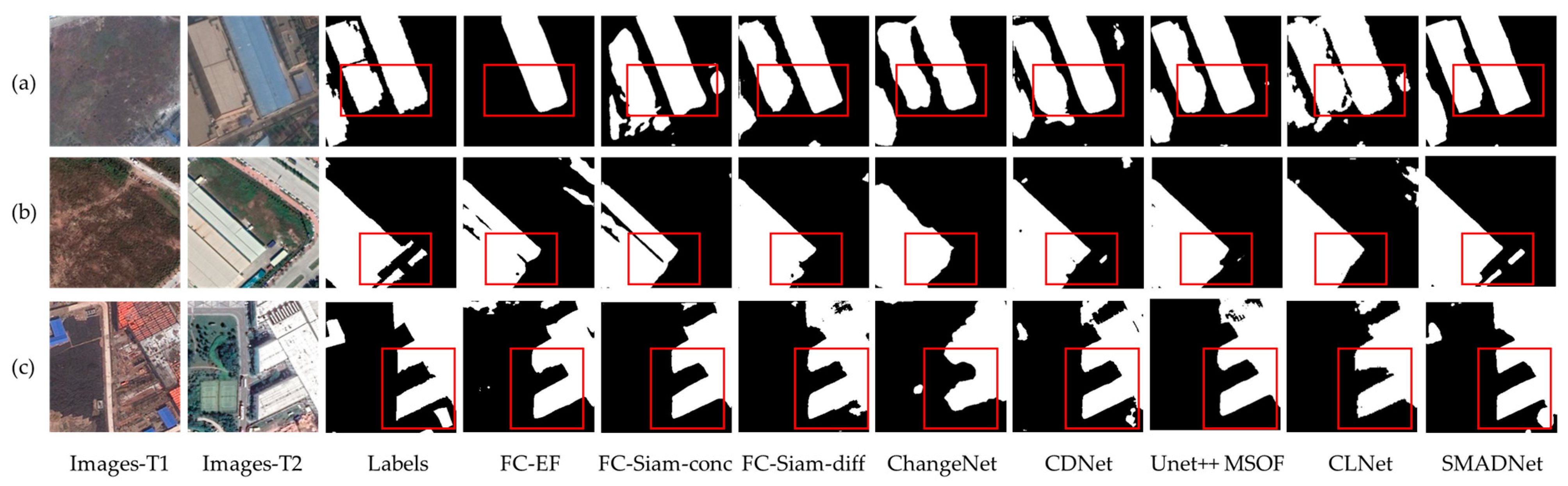
3.4.1. Experiments on GDSCD

The GDSCD dataset encompasses the suburban regions of Guangzhou, China, areas that have undergone intricate transformations. Given the complexity of the change scenes, we focused our BCD experiments on the GDSCD dataset. The outcomes of the detection using our proposed SMADNet, in comparison to other competing algorithms, are illustrated in Figure 8. Additionally, a quantitative comparison against these competing algorithms can be found in

Table 1. Quantitative evaluation results on GDSCD dataset with competing networks (unit: %).

Methods	P	R	F1	OA	IoU	MIoU	Kappa
FC-EF	61.50	78.70	69.05	96.27	52.72	74.41	67.09
FC-Siam-conc	62.17	82.50	70.90	96.54	54.92	75.66	69.10
FC-Siam-diff	77.16	80.15	78.63	97.16	64.78	80.89	77.11
ChangeNet	79.67	84.71	82.11	97.65	69.65	83.58	80.86
CDNet	74.07	81.59	77.65	97.11	63.46	80.21	76.11
Unet++MSOF	69.29	88.76	77.83	97.33	63.70	80.45	76.43
CLNet	71.63	79.41	75.32	96.82	60.41	78.54	73.63
SMADNet	88.64	87.35	87.99	98.36	78.56	88.41	87.11

.

The SMADNet approach, as proposed in our study, consistently yields superior detection outcomes on the GDSCD dataset, distinctly outclassing the performance of the other seven contender algorithms. It is crucial to note that the GDSCD dataset primarily captures extensive buildings and factories, many of which are closely knit. This contrasts sharply with the isolated, smaller structures predominantly found in the LEVIR-CD dataset. As evidenced by the metrics in Table 1, SMADNet excels in building change detection, showcasing an IoU of 78.56%, an MIoU of 88.41%, and an impressive OA of 98.36%. This IoU is notably 8.91% superior to that of ChangeNet, which stands as the closest competitor. Evidently, our method has significantly advanced the accuracy in detecting building changes compared to alternative techniques. With a precision rate that is 8.97% greater than that of ChangeNet, SMADNet surpasses all other examined methodologies.

In suburban settings, building detection is often complicated by the shadows cast by trees. Moreover, the sun’s position can introduce shadows that extend beyond building contours, leading to errors in boundary extraction. Nevertheless, our methodology effectively addresses these challenges, as illustrated in Figure 8. Observing Figure 8a, it becomes evident that buildings detected by SMADNet present a notable advantage in boundary precision. The extracted edges appear smooth and intact, devoid of any undue cohesion. Notably, regions that were overlooked in the original data are more comprehensively identified. In contrast, structures identified by competing algorithms often suffer from issues like edge cohesion, fragmentation, and omission of entire building structures. Figure 8b highlights that while other algorithms falter somewhat in recognizing smaller structures—often entirely omitting them, or detecting them incompletely or erroneously—SMADNet excels. It not only captures these smaller buildings more holistically but also essentially avoids any false detections. Lastly, as shown in Figure 8c, there is a significant contiguous structure that dominates nearly half the image. SMADNet’s detection results portray the majority of this building, especially sections like the upper right corner, without any missing gaps. The delineation is sharp, and the structure’s boundaries are well-defined. Though there is minor cohesion detected along the building’s lower right boundary and a smaller portion detected in the upper left corner, the overall representation remains commendably superior, especially when juxtaposed against results that miss these areas entirely.

3.4.2. Experiments on LEVIR-CD

First, we undertook experiments utilizing the LEVIR-CD dataset. The detection results acquired by SMADNet in juxtaposition with other competing algorithms are visualized in Figure 9, whereas a quantitative analysis with competing algorithms is presented in

Table 2. Quantitative evaluation results on LEVIR-CD dataset with competing networks (unit: %).

Methods	P	R	F1	OA	IoU	MIoU	Kappa
FC-EF	78.72	85.43	81.94	98.23	69.40	83.78	81.01
FC-Siam-conc	83.02	87.47	85.19	98.53	74.20	86.33	84.41
FC-Siam-diff	81.65	90.88	86.02	98.65	75.47	87.03	85.31
ChangeNet	82.56	84.40	83.47	98.33	76.30	84.95	82.59
CDNet	84.99	88.99	86.94	98.70	76.90	87.77	86.26
Unet++MSOF	86.26	90.23	88.20	98.87	79.50	89.16	87.99
CLNet	87.94	90.49	89.20	98.92	80.50	89.68	88.63
SMADNet	88.97	92.49	90.70	99.07	82.98	91.00	90.21

. Reviewing Table 1, SMADNet’s superior performance on the LEVIR-CD dataset becomes evident. Across all accuracy metrics, SMADNet surpasses the benchmark set by comparative methods. Specifically, the SMADNet methodology attains 82.98% and 91.0% for IoU and MIoU metrics. It registers improvements of 1.03%, 1.5%, and 0.15% over CLNet, the top-performing algorithm among the comparison group, across Precision, F1, and OA metrics, respectively. Additionally, it surpasses FC-Siam-diff by 1.61% in the Recall metric.

The LEVIR-CD dataset encompasses a diverse range of building types, emphasizing pertinent changes such as building expansion and degradation. As illustrated in Figure 9, this dataset captures transitions from terrains like soil and grass to more solid grounds or construction sites. Analyzing Figure 9a, we observe a high building density with minimal interspersed gaps. While the detection outcomes of several alternative algorithms display varying levels of cohesion, the SMADNet network’s results reveal a more comprehensive building detection, albeit with minor boundary cohesion. In the scenario presented in Figure 9b, where competitive algorithms depict the building in the upper left with a fragmented boundary and an incomplete structure, SMADNet delivers a more holistic edge detection with a fully recognized structure. Figure 9c showcases the results of other algorithms, which often present incomplete edges and artifacts within the building’s body. Given that buildings in this area are flanked by terrains sharing color attributes similar to rooftops and consistent imaging tones across temporal phases, many comparative algorithms err by deeming this as a static region, leading to variances in missed detections. In contrast, SMADNet captures a broader change region, underscoring our method’s enhanced generalization capability and robustness.

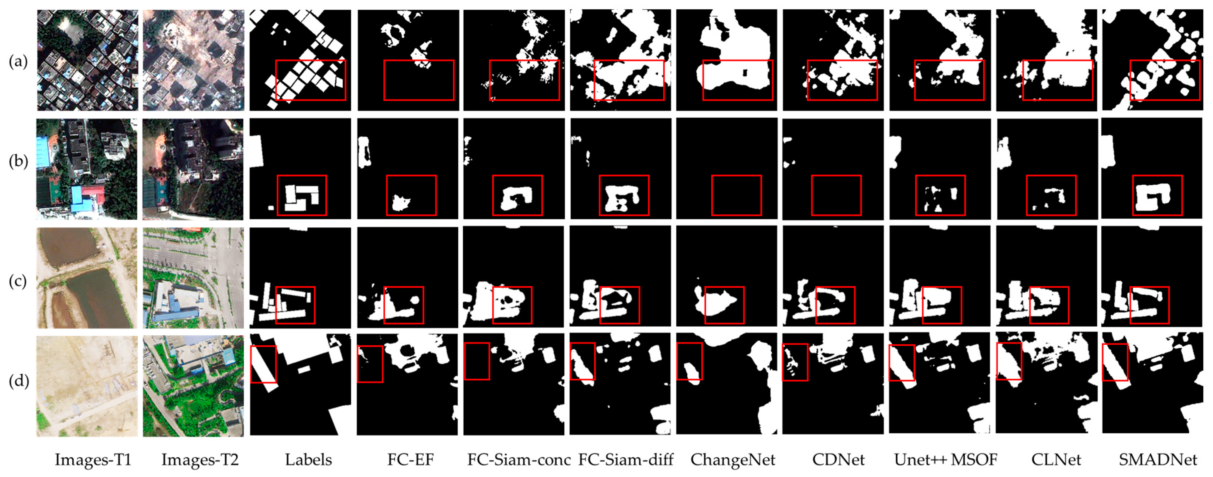
3.4.3. Experiments on HRCUS-CD

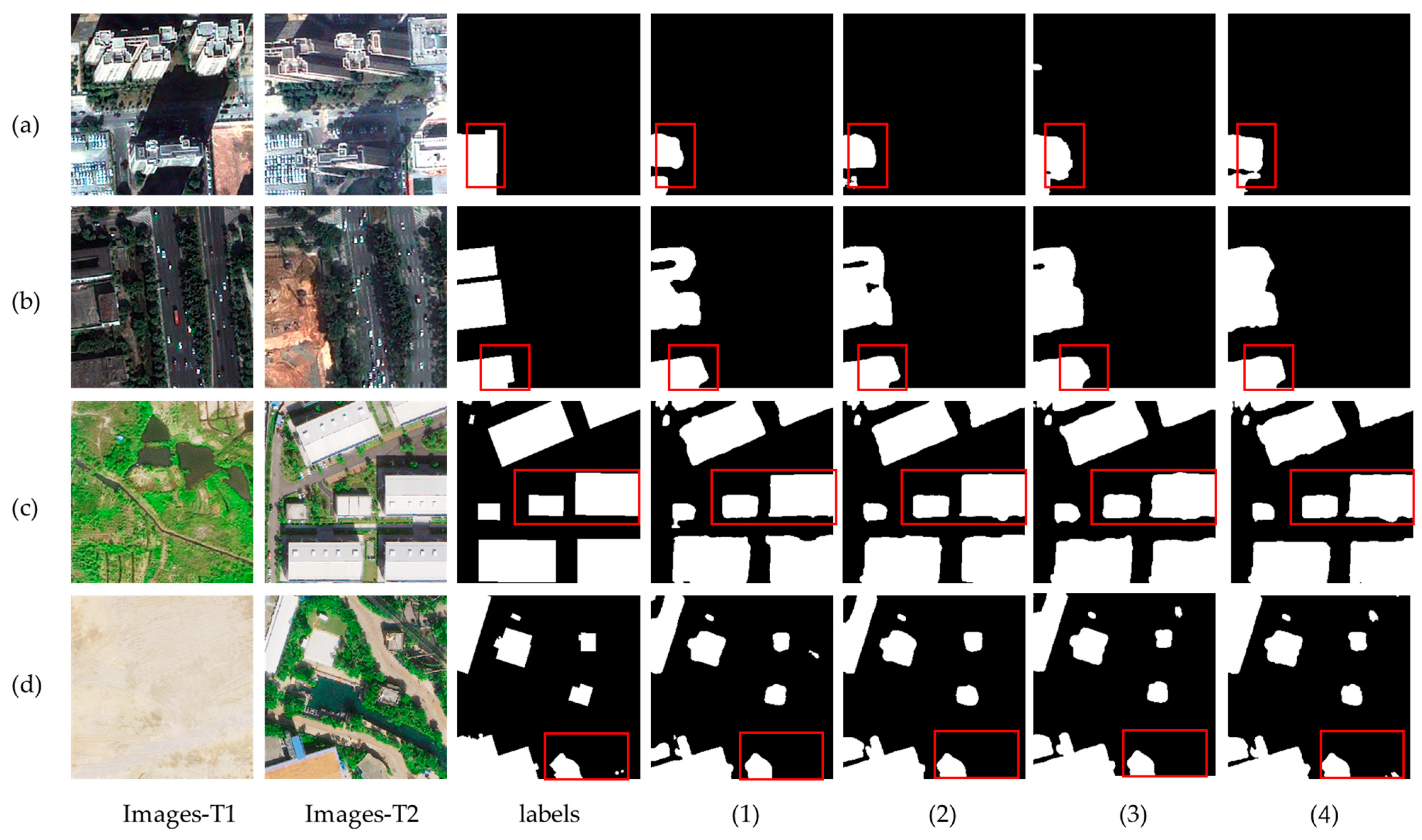
To further assess the detection capabilities of our method within intricate urban landscapes, we opted for the HRCUS-CD dataset sourced from Zhuhai, Guangdong, China. This dataset presents a contrast to the previously discussed GDSCD dataset, which primarily focuses on suburban settings. Comparative detection results, pitched between SMADNet and other competing algorithms, are depicted in Figure 10. In Figure 10a,b, the imagery is sourced from the Pleiades satellite, revealing an intricate urban terrain characterized by multifaceted building structures. On the other hand, Figure 10c,d are derived from the Worldview satellite’s imaging. These latter images, devoid of the intricate features evident in their predecessors, pose a relatively straightforward detection challenge.

Figure 10a showcases the detection outcomes for an urban village characterized by intricate changes. Most competing algorithms display less than optimal results, often failing to discern clear building boundaries. Small buildings are lumped together, and, as a consequence, it becomes challenging to differentiate specific building instances. Furthermore, these results are marred by a plethora of noise points. In stark contrast, the detection by SMADNet closely mirrors the actual scenario; the building outlines are predominantly distinct. Moreover, the demarcations of smaller building structures are more discernible and exhibit less adhesion compared to those discerned by other methods. This underscores SMADNet’s robust detection prowess even amidst multifaceted urban terrains. From Figure 10b, while the number of altered buildings is limited, primarily centered around petite factories, their surroundings present intricate detailing. SMADNet adeptly detects the evolving buildings, replicating their sizes fairly accurately. The boundaries extracted by SMADNet are notably more defined and align better with the labeled states.

In Figure 10c, a substantial transformation in land use is evident, transitioning from pond farmland to highways and industrial structures. The FC-Siam-conc approach struggles to delineate precise building boundaries, exhibiting pronounced adhesion issues. While the remaining methods avoid extensive adhesion, their extracted boundaries remain inconsistent, complicating the identification of specific building structures. Conversely, SMADNet’s detection presents clearer boundary definitions with minimal adhesion. Moreover, the coloration of the detected buildings closely mirrors the surrounding terrain. From Figure 10d, the initial image, T1, represents newly reclaimed land, whereas the subsequent image, T2, depicts an intricate blend of roads, vegetation, and trees. The primary challenge faced by comparative methods stems from the marked similarity in coloration between building rooftops and concrete pathways, resulting in incomplete detection of expansive structures. Such outcomes are marred by omissions, gaps, and notable adhesions. In stark contrast, SMADNet’s detection aligns well with the original labels. The structures identified by SMADNet are both regular and comprehensive. Furthermore, the spatial expanse of the detected buildings exceeds that of other methods, and incidences of missed details are significantly minimized.

Table 3. Quantitative evaluation results on HRCUS-CD dataset with competing networks (unit: %).

Methods	P	R	F1	OA	IoU	MIoU	Kappa
FC-EF	42.26	64.28	50.99	98.48	34.22	66.34	50.25
FC-Siam-conc	53.95	66.95	59.75	98.64	42.61	70.61	59.07
FC-Siam-diff	64.29	67.76	65.98	98.76	49.23	73.99	65.34
ChangeNet	55.24	67.09	60.59	98.65	43.46	71.05	59.91
CDNet	55.74	67.95	61.24	98.68	44.14	71.40	60.58
Unet++MSOF	61.10	70.06	65.27	98.78	48.45	73.61	64.65
CLNet	67.67	61.07	64.20	98.59	47.28	72.92	63.48

provides a quantitative evaluation, juxtaposing our proposed methods against competing algorithms on the HRCUS-CD dataset. As delineated in Table 3, SMADNet consistently surpasses its competitors, clinching the apex scores across all evaluated metrics. Specifically, our methodology registers the preeminent IoU and MIoU scores at 59.36% and 79.19%, respectively. These scores stand 10.13% and 5.20%, respectively, above the subsequent best performer, FC-Siam-diff. Delving deeper, the FC-Siam-diff method attains an IoU of 49.23% and an MIoU of 73.99%, marking it as the best-performing among FC baselines. This underscores the efficacy of the Siamese structure. The Unet++ MSOF occupies the third position, recording an IoU of 48.45% and an MIoU of 73.61%. Intriguingly, a deviation from the GDSCD dataset results is observed: on the HRCUS-CD dataset, FC-Siam-diff outshines ChangeNet. This might be attributed to the nuanced intricacies of the HRCUS-CD dataset, where varying features might induce information omissions.

4. Discussion

In this section, we conduct ablation experiments on the GDSCD, LEVIR-CD and HRCUS-CD datasets to verify the effectiveness of the MCFFM, CADM, and DS in SMADNet. We define the SMADNet with the removed above module as the Baseline method. The ablation results images are shown in Figure 11, and the quantitative results are shown in

Table 4. Quantitative evaluation results of ablation experiments on datasets (unit: %).

Datasets	Baseline	MCFFM	CADM	DS	IoU	OA	F1	Kappa
GDSCD	✓				72.61	97.85	84.13	82.98
	✓	✓			74.01	97.97	85.07	83.98
	✓	✓	✓		76.13	98.25	86.45	85.52
	✓	✓	✓	✓	78.56	98.36	87.99	87.11
LEVIR-CD	✓				78.95	98.77	88.24	87.59
	✓	✓			79.82	98.90	88.78	88.2
	✓	✓	✓		81.93	99.01	90.07	89.55
	✓	✓	✓	✓	82.98	99.07	90.70	90.21
HRCUS-CD	✓				54.96	98.85	70.93	70.35
	✓	✓			56.84	98.98	72.48	71.96
	✓	✓	✓		57.08	98.96	72.68	72.15
	✓	✓	✓	✓	59.36	99.02	74.50	74.00

. From Figure 11 and Table 4, it can be seen that the introduction of three modules can further improve the accuracy of building change detection. Baseline+MCFFM, Baseline+MCFFM + CADM, and SAMDNet are better than the baseline method.

As can be seen in Figure 11a,b, the introduction of modules is more favorable for feature extraction to suppress pseudo-variation and to reduce null detection in complex urban scenes. The image pairs in Figure 11a have been strictly registered, but the buildings present visual differences due to satellite imaging. Our SMADNet network does not experience false detections, which means it can suppress pseudo-variation effectively. From Figure 11c,d, it can be seen that the inclusion of each module can effectively suppress the effect of tree shadows on the detection, presumably due to the fact that the CADM module can emphasize the target features and suppress the weights of irrelevant pixels. All the above results demonstrate the effectiveness of the modules used by the network for the detection of changing buildings.

From Table 4, we observe that the accuracy metrics show a generally increasing trend when proposed modules are added. It is worth noting that, compared to the baseline, the IoU of the three datasets improved by 5.95%, 4.42%, and 4.4%, and the MIoU improved by 3.25%, 2.17%, and 2.29%, respectively, indicating the gainfulness of the combination of the three modules on the detection performance.

5. Conclusions

In this study, we introduce the SMADNet for building CD tasks, comprising the SWN and CDN components. The SMADNet leverages the MCFFM to consolidate multiscale contextual data and amplify the connection between bitemporal imagery. We present the CADM, which is a fusion of the SAM and CAM. This amalgamation accentuates the precision on pixels of interest and bolsters the discernment of change features across both channel and spatial aspects. For an optimized training trajectory, the Deep Supervision (DS) strategy is deployed, enhancing the network’s adaptability to salient features. Empirical evaluations demonstrate that our SMADNet surpasses other state-of-the-art (SOTA) methods across the GDSCD, LEVIR-CD, and HRCUS-CD datasets. It adeptly addresses challenges like vast target scale fluctuations, intricate urban landscapes, and obstructions such as trees and shadows. The efficacy of the proposed modules is corroborated through detailed ablation studies. Looking ahead, our focus will be on refining the model’s design and identifying the most compatible attention modules and multiscale fusion mechanisms.

References

1. Singh, A. Review article digital change detection techniques using remotely-sensed data. Int. J. Remote Sens. 1989, 10, 989–1003. [Google Scholar] [CrossRef]
2. Demir, B.; Bovolo, F.; Bruzzone, L. Updating land-cover maps by classification of image time series: A novel change-detection-driven transfer learning approach. IEEE Trans. Geosci. Remote Sens. 2012, 51, 300–312. [Google Scholar] [CrossRef]
3. Walter, V. Object-based classification of remote sensing data for change detection. ISPRS J. Photogramm. Remote Sens. 2004, 58, 225–238. [Google Scholar] [CrossRef]
4. Jimenez-Sierra, D.A.; Benítez-Restrepo, H.D.; Vargas-Cardona, H.D.; Chanussot, J. Graph-based data fusion applied to: Change detection and biomass estimation in rice crops. Remote Sens. 2020, 12, 2683. [Google Scholar] [CrossRef]
5. Gong, M.; Zhao, J.; Liu, J.; Miao, Q.; Jiao, L. Change detection in synthetic aperture radar images based on deep neural networks. IEEE Trans. Neural Netw. Learn. Syst. 2015, 27, 125–138. [Google Scholar] [CrossRef]
6. Ji, S.; Wei, S.; Lu, M. Fully convolutional networks for multisource building extraction from an open aerial and satellite imagery data set. IEEE Trans. Geosci. Remote Sens. 2018, 57, 574–586. [Google Scholar] [CrossRef]
7. Zheng, H.; Gong, M.; Liu, T.; Jiang, F.; Zhan, T.; Lu, D.; Zhang, M. HFA-Net: High frequency attention siamese network for building change detection in VHR remote sensing images. Pattern Recognit. 2022, 129, 108717. [Google Scholar] [CrossRef]
8. Asokan, A.; Anitha, J.J. Change detection techniques for remote sensing applications: A survey. Earth Sci. Inform. 2019, 12, 143–160. [Google Scholar] [CrossRef]
9. Awrangjeb, M.; Gilani, S.A.N.; Siddiqui, F.U. An effective data-driven method for 3-d building roof reconstruction and robust change detection. Remote Sens. 2018, 10, 1512. [Google Scholar] [CrossRef]
10. Zhu, Q.; Guo, X.; Li, Z.; Li, D. A review of multi-class change detection for satellite remote sensing imagery. Geo-Spat. Inf. Sci. 2022, 1–15. [Google Scholar] [CrossRef]
11. Hussain, M.; Chen, D.; Cheng, A.; Wei, H.; Stanley, D. Change detection from remotely sensed images: From pixel-based to object-based approaches. ISPRS J. Photogramm. Remote Sens. 2013, 80, 91–106. [Google Scholar] [CrossRef]
12. Zhang, Y.; Peng, D.; Huang, X. Object-based change detection for VHR images based on multiscale uncertainty analysis. IEEE Geosci. Remote Sens. Lett. 2017, 15, 13–17. [Google Scholar] [CrossRef]
13. Zhang, C.; Li, G.; Cui, W. High-resolution remote sensing image change detection by statistical-object-based method. IEEE J. Sel. Top. Appl. Earth Obs. Remote Sens. 2018, 11, 2440–2447. [Google Scholar] [CrossRef]
14. Gil-Yepes, J.L.; Ruiz, L.A.; Recio, J.A.; Balaguer-Beser, Á.; Hermosilla, T. Description and validation of a new set of object-based temporal geostatistical features for land-use/land-cover change detection. ISPRS J. Photogramm. Remote Sens. 2016, 121, 77–91. [Google Scholar] [CrossRef]
15. Qin, Y.; Niu, Z.; Chen, F.; Li, B.; Ban, Y. Object-based land cover change detection for cross-sensor images. Int. J. Remote Sens. 2013, 34, 6723–6737. [Google Scholar] [CrossRef]
16. Ma, L.; Li, M.; Blaschke, T.; Ma, X.; Tiede, D.; Cheng, L.; Chen, Z.; Chen, D. Object-based change detection in urban areas: The effects of segmentation strategy, scale, and feature space on unsupervised methods. Remote Sens. 2016, 8, 761. [Google Scholar] [CrossRef]
17. Bai, T.; Wang, L.; Yin, D.; Sun, K.; Chen, Y.; Li, W.; Li, D. Deep learning for change detection in remote sensing: A review. Geo-Spat. Inf. Sci. 2022, 1–27. [Google Scholar] [CrossRef]
18. Deng, J.S.; Wang, K.; Deng, Y.H.; Qi, G.J. PCA-based land-use change detection and analysis using multitemporal and multisensor satellite data. Int. J. Remote Sens. 2008, 29, 4823–4838. [Google Scholar] [CrossRef]
19. Wu, C.; Du, B.; Cui, X.; Zhang, L. A post-classification change detection method based on iterative slow feature analysis and Bayesian soft fusion. Remote Sens. Environ. 2017, 199, 241–255. [Google Scholar] [CrossRef]
20. Ma, L.; Liu, Y.; Zhang, X.; Ye, Y.; Yin, G.; Johnson, B.A. Deep learning in remote sensing applications: A meta-analysis and review. ISPRS J. Photogramm. Remote Sens. 2019, 152, 166–177. [Google Scholar] [CrossRef]
21. Wang, Q.; Zhang, X.; Chen, G.; Dai, F.; Gong, Y.; Zhu, K. Change detection based on Faster R-CNN for high-resolution remote sensing images. Remote Sens. Lett. 2018, 9, 923–932. [Google Scholar] [CrossRef]
22. Long, Y.; Xia, G.S.; Li, S.; Yang, W.; Yang, M.Y.; Zhu, X.X.; Zhang, L.; Li, D. On creating benchmark dataset for aerial image interpretation: Reviews, guidances, and million-aid. IEEE J. Sel. Top. Appl. Earth Obs. Remote Sens. 2021, 14, 4205–4230. [Google Scholar] [CrossRef]
23. Ding, Q.; Shao, Z.; Huang, X.; Altan, O. DSA-Net: A novel deeply supervised attention-guided network for building change detection in high-resolution remote sensing images. Int. J. Appl. Earth Obs. Geoinf. 2021, 105, 102591. [Google Scholar] [CrossRef]
24. Daudt, R.C.; Le Saux, B.; Boulch, A.; Gousseau, Y. Urban change detection for multispectral earth observation using convolutional neural networks. In Proceedings of the IGARSS 2018—2018 IEEE International Geoscience and Remote Sensing Symposium, Valencia, Spain, 22–27 July 2018; pp. 2115–2118. [Google Scholar]
25. Long, J.; Shelhamer, E.; Darrell, T. Fully convolutional networks for semantic segmentation. In Proceedings of the IEEE Conference on Computer Vision and Pattern Recognition, Boston, MA, USA, 7–12 June 2015; pp. 3431–3440. [Google Scholar]
26. Ronneberger, O.; Fischer, P.; Brox, T. U-net: Convolutional networks for biomedical image segmentation. In Medical Image Computing and Computer-Assisted Intervention—MICCAI 2015, Proceedings of the 18th International Conference, Munich, Germany, 5–9 October 2015; Proceedings, Part III 18; Springer International Publishing: Cham, Switzerland, 2015; pp. 234–241. [Google Scholar]
27. Ji, S.; Shen, Y.; Lu, M.; Zhang, Y. Building instance change detection from large-scale aerial images using convolutional neural networks and simulated samples. Remote Sens. 2019, 11, 1343. [Google Scholar] [CrossRef]
28. Zhan, Y.; Fu, K.; Yan, M.; Sun, X.; Wang, H.; Qiu, X. Change detection based on deep siamese convolutional network for optical aerial images. IEEE Geosci. Remote Sens. Lett. 2017, 14, 1845–1849. [Google Scholar] [CrossRef]
29. Liu, Y.; Pang, C.; Zhan, Z.; Zhang, X.; Yang, X. Building change detection for remote sensing images using a dual-task constrained deep siamese convolutional network model. IEEE Geosci. Remote Sens. Lett. 2020, 18, 811–815. [Google Scholar] [CrossRef]
30. Daudt, R.C.; Le Saux, B.; Boulch, A. Fully convolutional siamese networks for change detection. In Proceedings of the 2018 25th IEEE International Conference on Image Processing (ICIP), Athens, Greece, 7–10 October 2018; pp. 4063–4067. [Google Scholar]
31. Zhao, H.; Shi, J.; Qi, X.; Wang, X.; Jia, J. Pyramid scene parsing network. In Proceedings of the IEEE Conference on Computer Vision and Pattern Recognition, Honolulu, HI, USA, 21–26 July 2017; pp. 2881–2890. [Google Scholar]
32. Chen, L.C.; Papandreou, G.; Schroff, F.; Adam, H. Rethinking atrous convolution for semantic image segmentation. arXiv 2017, arXiv:1706.05587. [Google Scholar]
33. Varghese, A.; Gubbi, J.; Ramaswamy, A.; Balamuralidhar, P. ChangeNet: A deep learning architecture for visual change detection. In Proceedings of the European Conference on Computer Vision (ECCV) Workshops, Munich, Germany, 8–14 September 2018. [Google Scholar]
34. Jin, W.D.; Xu, J.; Han, Q.; Zhang, Y.; Cheng, M.M. CDNet: Complementary depth network for RGB-D salient object detection. IEEE Trans. Image Process. 2021, 30, 3376–3390. [Google Scholar] [CrossRef]
35. Zhou, Z.; Rahman Siddiquee, M.M.; Tajbakhsh, N.; Liang, J. Unet++: A nested u-net architecture for medical image segmentation. In Deep Learning in Medical Image Analysis and Multimodal Learning for Clinical Decision Support, Proceedings of the 4th International Workshop, DLMIA 2018, and 8th International Workshop, ML-CDS 2018, Held in Conjunction with MICCAI 2018, Granada, Spain, 20 September 2018; Proceedings 4; Springer International Publishing: Cham, Switzerland, 2018; pp. 3–11. [Google Scholar]
36. Peng, D.; Zhang, Y.; Guan, H. End-to-end change detection for high resolution satellite images using improved UNet++. Remote Sens. 2019, 11, 1382. [Google Scholar] [CrossRef]
37. Zheng, Z.; Wan, Y.; Zhang, Y.; Xiang, S.; Peng, D.; Zhang, B. CLNet: Cross-layer convolutional neural network for change detection in optical remote sensing imagery. ISPRS J. Photogramm. Remote Sens. 2021, 175, 247–267. [Google Scholar] [CrossRef]
38. Shi, Q.; Liu, M.; Li, S.; Liu, X.; Wang, F.; Zhang, L. A deeply supervised attention metric-based network and an open aerial image dataset for remote sensing change detection. IEEE Trans. Geosci. Remote Sens. 2021, 60, 1–16. [Google Scholar] [CrossRef]
39. Chen, J.; Yuan, Z.; Peng, J.; Chen, L.; Huang, H.; Zhu, J.; Liu, Y.; Li, H. DASNet: Dual attentive fully convolutional Siamese networks for change detection in high-resolution satellite images. IEEE J. Sel. Top. Appl. Earth Obs. Remote Sens. 2020, 14, 1194–1206. [Google Scholar] [CrossRef]
40. Vaswani, A.; Shazeer, N.; Parmar, N.; Uszkoreit, J.; Jones, L.; Gomez, A.N.; Kaiser, Ł.; Polosukhin, I. Attention is all you need. Adv. Neural Inf. Process. Syst. 2017, 30. [Google Scholar]
41. Bandara, W.G.C.; Patel, V.M. A transformer-based siamese network for change detection. In Proceedings of the IGARSS 2022—2022 IEEE International Geoscience and Remote Sensing Symposium, Kuala Lumpur, Malaysia, 17–22 July 2022; pp. 207–210. [Google Scholar]
42. Wang, D.; Chen, X.; Guo, N.; Yi, H.; Li, Y. STCD: Efficient Siamese transformers-based change detection method for remote sensing images. Geo-Spat. Inf. Sci. 2023, 1–20. [Google Scholar] [CrossRef]
43. Shi, W.; Zhang, M.; Zhang, R.; Chen, S.; Zhan, Z. Change detection based on artificial intelligence: State-of-the-art and challenges. Remote Sens. 2020, 12, 1688. [Google Scholar] [CrossRef]
44. Dong, H.; Ma, W.; Wu, Y.; Gong, M.; Jiao, L. Local descriptor learning for change detection in synthetic aperture radar images via convolutional neural networks. IEEE Access 2018, 7, 15389–15403. [Google Scholar] [CrossRef]
45. Gong, M.; Yang, H.; Zhang, P. Feature learning and change feature classification based on deep learning for ternary change detection in SAR images. ISPRS J. Photogramm. Remote Sens. 2017, 129, 212–225. [Google Scholar] [CrossRef]
46. Peng, D.; Bruzzone, L.; Zhang, Y.; Guan, H.; Ding, H.; Huang, X. SemiCDNet: A semisupervised convolutional neural network for change detection in high resolution remote-sensing images. IEEE Trans. Geosci. Remote Sens. 2020, 59, 5891–5906. [Google Scholar] [CrossRef]
47. Chen, H.; Shi, Z. A spatial-temporal attention-based method and a new dataset for remote sensing image change detection. Remote Sens. 2020, 12, 1662. [Google Scholar] [CrossRef]
48. Zhang, J.; Shao, Z.; Ding, Q.; Huang, X.; Wang, Y.; Zhou, X.; Li, D. AERNet: An attention-guided edge refinement network and a dataset for remote sensing building change detection. IEEE Trans. Geosci. Remote Sensing 2023, 61, 5617116. [Google Scholar] [CrossRef]
49. He, K.; Zhang, X.; Ren, S.; Sun, J. Deep residual learning for image recognition. In Proceedings of the IEEE Conference on Computer Vision and Pattern Recognition, Las Vegas, NV, USA, 27–30 June 2016; pp. 770–778. [Google Scholar]
Figure 1. Overview of the SMADNet.
Remotesensing 15 05127 g001
Figure 2. The Structure of MCFFM.
Remotesensing 15 05127 g002
Figure 3. The Structure of CADM.
Remotesensing 15 05127 g003
Figure 4. The Structure of NDB.
Remotesensing 15 05127 g004
Figure 5. The Structure of Channel Attention Mechanism.
Remotesensing 15 05127 g005
Figure 6. The Structure of Spatial Attention Mechanism.
Remotesensing 15 05127 g006
Figure 7. Example samples (256 × 256). (a) GDSCD; (b) LEVIR-CD; (c) HRCUS-CD.
Remotesensing 15 05127 g007
Figure 8. Visual comparison of results on the GDSCD dataset with (ac) FC-EF, FC-Siam-conc, FC-Siam-diff, ChangeNet, CDNet, Unet++ MSOF, CLNet, and the proposed SMADNet.
Remotesensing 15 05127 g008
Figure 9. Visual comparison of resultson the LEVIR-CD dataset with (ac) FC-EF, FC-Siam-conc, FC-Siam-diff, ChangeNet, CDNet, Unet++MSOF, CLNet, and the proposed SMADNet.
Remotesensing 15 05127 g009
Figure 10. Visual comparison of results on the HRCUS-CD dataset with FC-EF, FC-Siam-conc, FC-Siam-diff, ChangeNet, CDNet, Unet++MSOF, CLNet, and the proposed SMADNet.
Remotesensing 15 05127 g010
Figure 11. Examples of the ablation experiments on the proposed method from HRCUS-CD dataset: (1) Baseline; (2) Baseline + MCFFM; (3) Baseline + MCFFM + CADM; (4) SMADNet.
Remotesensing 15 05127 g011