NMS-Free Oriented Object Detection Based on Channel Expansion and Dynamic Label Assignment in UAV Aerial Images

Abstract

Object detection in unmanned aerial vehicle (UAV) aerial images has received extensive attention in recent years. The current mainstream oriented object detection methods for aerial images often suffer from complex network structures, slow inference speeds, and difficulties in deployment. In this paper, we propose a fast and easy-to-deploy oriented detector for UAV aerial images. First, we design a re-parameterization channel expansion network (RE-Net), which enhances the feature representation capabilities of the network based on the channel expansion structure and efficient layer aggregation network structure. During inference, RE-Net can be equivalently converted to a more streamlined structure, reducing parameters and computational costs. Next, we propose DynamicOTA to adjust the sampling area and the number of positive samples dynamically, which solves the problem of insufficient positive samples in the early stages of training. DynamicOTA improves detector performance and facilitates training convergence. Finally, we introduce a sample selection module (SSM) to achieve NMS-free object detection, simplifying the deployment of our detector on embedded devices. Extensive experiments on the DOTA and HRSC2016 datasets demonstrate the superiority of the proposed approach.

1. Introduction

Object detection is an important task in computer vision. With the rapid development of deep learning, several models based on convolutional neural networks (CNN) have been proposed to achieve high-performance detection, including YOLO series [1,2,3,4], R-CNN series [5,6,7,8], RetinaNet [9], FCOS [10] and CenterNet [11]. Object detection in unmanned aerial vehicle (UAVs) images has promising applications and attracts much attention.

Different from objects in natural scenes, objects in UAV aerial imagery are often distributed with large scale variations, leading to great challenges in accurate detection. In addition, small objects often lack sufficient information about their appearance, making them more challenging to identify. Therefore, current object detection methods in aerial images tend to employ complex network structures and a larger number of parameters to achieve higher detection accuracy. As shown in Figure 1, the AlignConv in S${}^2$ANet [12] and the RoI Transformer [13] improve the accuracy of aerial image detection, but impose computational costs. In particular, implementing these specialized structures on embedded devices is difficult. Due to the limited size of UAVs, detectors need to be deployed on an embedded device, which requires a streamlined detector.

In addition, objects with arbitrary orientation make it difficult to represent the boundaries with a horizontal bounding box (HBB). The aerial object detection task converts the HBB into an oriented bounding box (OBB) by adding a rotation angle [12,14,15,16,17,18,19,20,21,22]. This makes it necessary to calculate the rotated intersection over union (IoU) in training and inference. However, the calculation of rotated IoU is complex, making the rotated non-maximum suppression (NMS) algorithm difficult to implement on embedded devices and increasing inference-time costs.

In this paper, we propose a fast and easy-to-deploy oriented detector for UAV aerial images. Our work focuses on the balance between speed and accuracy. First, to increase the feature extraction capacity of our network, we design a re-parameterization channel expansion network (RE-Net), which expands the features to channels of different dimensions. During inference, RE-Net can be equivalently converted to a more streamlined structure, reducing parameters and computation. In addition, we introduce the efficient layer aggregation network (ELAN) structure to improve detection accuracy.

We propose an advanced dynamic label assignment strategy called DynamicOTA, which adjusts the sampling area and the number of positive samples based on training progress. DynamicOTA enables a transition from dense to sparse label assignment, accelerating training convergence and increasing detection accuracy with no extra inference-time cost. This is in line with our goal of developing a fast, easy-to-deploy oriented detector.

Furthermore, we suggest that the calculation process of rotated IoU increases the difficulty of network deployment and the inference-time cost. Accordingly, we introduce a sample selection module (SSM) to fully enable end-to-end object detection, eliminating the need for NMS. The SSM consists of convolutional layers and has a simple structure.

To summarize, the main contributions of this paper are as follows:

(1)

We propose a fast and easy-to-deploy single-stage oriented detector for aerial images. Our method is both anchor-free and NMS-free and achieves competitive performance in both speed and accuracy. Moreover, we deploy our detector on the NVIDIA Xavier Jetson NX, achieving real-time inference speeds.

(2)

We design an RE-Net which expands the features to channels of different dimensions to enhance the feature representation capacity and allows significant reduction in the computation in inference. In addition, we implement a fully end-to-end OBB object detection based on the SSM, which reduces the difficulty of network deployment on embedded devices.

(3)

DynamicOTA is proposed to adjust the number of positive samples adaptively based on the training progress, solving the problem of insufficient positive samples at the early stage of SimOTA training, and improving the convergence speed of network and the detection accuracy with no extra inference-time cost.

The rest of this paper is organized as follows. Section 2 reviews the related work of generic object detection and oriented object detection in aerial images. Section 3 introduces our method in detail. Section 4 shows the ablation experiments of the proposed methods and the performance on different datasets. Section 5 concludes the paper.

2. Related Work

2.1. Generic Object Detection

Object detection has achieved significant advancements in recent years due to the introduction of CNN methods. Object detection methods are generally classified into two categories: two-stage detectors and single-stage detectors. The two-stage detectors, such as R-CNN [5], Fast R-CNN [6], Faster R-CNN [7], and R-FCN [23], generate candidate regions and subsequently perform classification and regression to obtain the final detections. Although these detectors offer higher accuracy, the division of the object detection task into two phases adversely impacts the network’s real-time performance.

In contrast, single-stage detectors conduct a more efficient detection that processes the entire image without generating candidate regions, leading to improved inference speed. The single-stage detectors include the YOLO series [1,2,3,4], SSD [24], RetinaNet [9] and FCOS [10], which demonstrated remarkable performance in various object detection tasks, providing a balance between accuracy and speed. As a result, single-stage detectors gained popularity in applications requiring real-time object detection and low-latency processing. YOLOX [1] is a state-of-the-art, anchor-free object detection network with significant speed and accuracy advantages over other object detection networks. Therefore, in this paper, we used YOLOX as a benchmark framework for detecting UAV aerial image objects.

2.2. Oriented Object Detection in Aerial Images

Object detection in aerial images has received extensive attention due to its wide range of application scenarios. With the significant breakthrough by CNN methods, object detection in aerial images has also made considerable progress. The current oriented detector is generally modified from the anchor-base HBB detector. Typically, these detectors generate oriented anchor boxes to learn orientation information and regress the offset between the object and anchor boxes. Early methods used anchors with multiple angles and aspect ratios to detect oriented objects [25,26]. However, preset overloading of anchor boxes generates too many detections and increases the time consumed. To avoid presetting a large number of anchors, the RoI transformer [13] proposes an RRoI learning module and RRoI warping to realize the transformation of HRoIs into RRoIs and then extract rotation invariant features. R${}^3$Det [27] and S${}^2$ANet [12] align the features between the horizontal receptive field and the OBB, addressing the inconsistency problem between classification and regression. ReDet [16] introduces rotation invariant convolution into the model and uses RiRoI Align to extract rotation invariant features. Oriented R-CNN [17] achieves oriented object detection based on an oriented region proposal network. CFC-Net [15] improves performance by building features suitable for classification and regression tasks, respectively.

Anchor-base methods usually require manual preset boxes, which not only introduces additional hyperparameters and computations, but also directly affects the performance of the model. Compared with anchor-based methods, anchor-free methods remove preset boxes and prior information, making them more adaptable than anchor-based methods. For example, O${}^2$-DNet [28] predicts the center point and a pair of intermediate lines to represent objects, eliminating the need for NMS and greatly simplifying the oriented detector. BBAVectors [29] and PolarDet [30] define the OBB with BBAVectors and polar coordinates, respectively. FCOSR [14] implements oriented object detection in a simple structure. Oriented RepPoints [31] and PIoU [32] use more efficient optimization strategies and different forms to represent OBB. The YOLOX object detection network used in this paper is an anchor-free method, which has a typical advantage.

3. The Proposed Method

The overall framework of our method is illustrated in Figure 2. The network directly predicts the objects’ center points (including x and y coordinates), width, height, IoU, and rotation angle. We propose several techniques to improve YOLOX for fast and accurate oriented object detection, including the RE-Net and the DynamicOTA. Additionally, we add the SSM that enables full end-to-end object detection, eliminating the need for NMS. The following sections provide detailed descriptions of these modules.

3.1. Re-Parameterization Channel Expansion Network

Objects in aerial images are densely arranged, with large-scale variations and arbitrary orientations, making it difficult to detect objects accurately. The detector needs to extract high-level semantic information and features of the objects in the images for accurate object localization and classification. At the same time, UAVs are restricted to carrying embedded devices, limiting the parameters and computational load of the network. Therefore, improving the network’s feature extraction capability while meeting the requirements of implementing on embedded devices requires us to develop a high-accuracy, real-time UAV aerial object detection algorithm.

RepVGG [33] improves the accuracy of the model without increasing the inference time by equivalently converting parallel 1 × 1 and 3 × 3 convolutions and identity connections into 3 × 3 convolutions. This method, called structural re-parameterization, streamlines the model structure and reduces the computational load. Linear over-parameterization [34] converts the cascaded 1 × 1 and 3 × 3 convolutions into equivalent 3 × 3 convolutions and shows excellent performance.

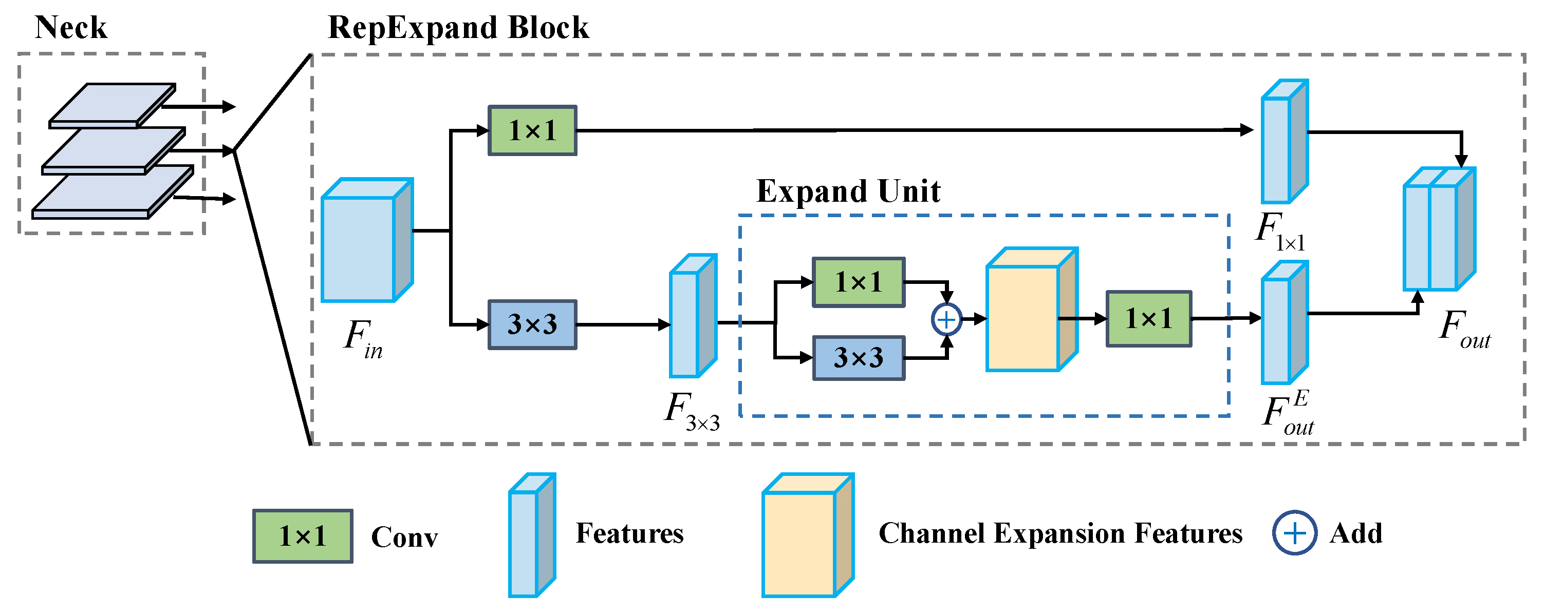
Inspired by these works, we design a novel re-parameterization expand block (RepExpand Block), with its structure illustrated in Figure 3. Given the input feature map from Neck $F_{in}\in R^{\mathbb{C}\times H\times W}$, we first reduce the input features to half their channel size in two different branches with 1 × 1 and 3 × 3 convolutions, respectively:

$$F_{1\times 1}={Conv}_{1\times 1}BNAct\left(F_{\mathrm{in}}\right),F_{3\times 3}={Conv}_{3\times 3}BNAct\left(F_{\mathrm{in}}\right),$$

(1)

in which $F_{1\times 1},F_{3\times 3}\in R^{0.5\ast \mathbb{C}\times H\times W}$, ConvBNAct denote the performing of convolution layer, batch normalization layer and activation function in series.

Next, we compute the enhanced features constructed by the Expand Unit based on $F_{3\times 3}$:

$$F_{out}^E=ExpandUnit\left(F_{3\times 3}\right),$$

(2)

in which $F_{out}^E\in R^{0.5\ast \mathbb{C}\times H\times W}$. The output of the RepExpand Block is the concatenation of $F_{out}^E$ and $F_{1\times 1}$:

$$F_{out}=cat\left(F_{out}^E,F_{1\times 1}\right),$$

(3)

in which $F_{out}\in R^{\mathbb{C}\times H\times W}$. The key element of the RepExpand block is the Expand Unit, as shown in Figure 4, which expands the input feature in the channel dimension by a factor of E with the convolutions of $3\times 3$ and $1\times 1$. This structure is designed to project features from a low-dimensional space into a higher-dimensional space, thus enhancing the network’s feature representation capability and consequently improving the accuracy of aerial object detection.

In the training phase, the Expand Unit’s structure is illustrated in Figure 4a. Given the input feature map of Expand Unit $F_{in}^E\in R^{C\times H\times W}$($F_{in}^E=F_{3\times 3}$ in Figure 3, and $C=0.5\mathbb{C}$), we expand the feature channel to $E\ast C$ as follows:

$$F_{1\times 1}^E={Conv}_{1\times 1}BN\left(F_{in}^E\right),F_{3\times 3}^E={Conv}_{3\times 3}BN\left(F_{in}^E\right),$$

(4)

in which $F_{1\times 1}^E,F_{3\times 3}^E\in R^{E\ast C\times H\times W}$. The output feature maps of the parallel 3 × 3 and 1 × 1 convolutions are then added, and the channels are finally narrowed to C by 1 × 1 convolution to obtain the output of the Expand Unit:

$$F_{\mathrm{out}}^E={Conv}_{1\times 1}BNAct\left(F_{1\times 1}^E+F_{3\times 3}^E\right),$$

(5)

where $F_{out}^E\in R^{C\times H\times W}$. This design also resembles an inverted residual structure [35], which enhances the ability of gradient propagation across the Expand Unit and improves network performance.

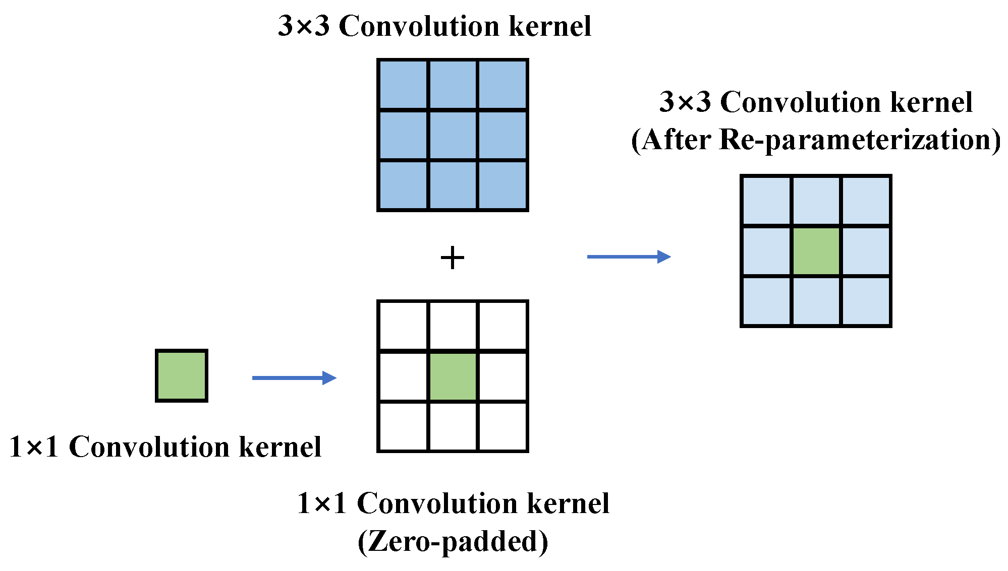
During the inference phase, the Expand Unit can be transformed into a single convolutional layer, significantly reducing parameters and computational load. As shown in Figure 5, the parallel 1 × 1 convolution kernel is zero-padded to a 3 × 3 size and combined with the 3 × 3 convolution kernel, achieving structural re-parameterization transformation [33]. The transformed structure is shown in Figure 4b.

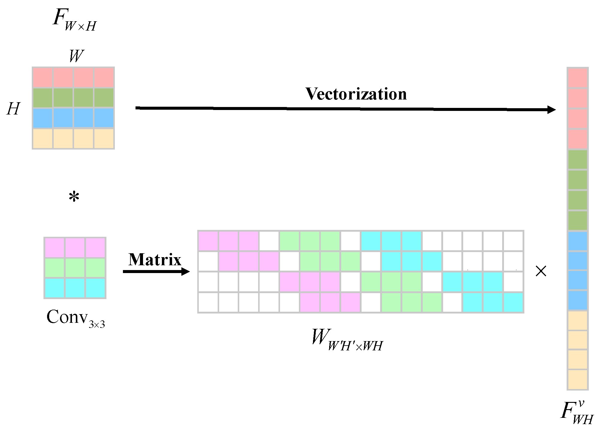
We next employ the linear over-parameterization method to further simplify the structure and reduce the parameters and computational load. As shown in Figure 6, the convolution operation is expressed in the matrix form. Specifically, we let $F_{C\times W\times H}$ denote the input feature map, and ${Conv}_{3\times 3}$ denote the convolution operation. The convolution process can be formulated in the matrix as follows [34]:

$${Conv}_{3\times 3}\left(F_{C\times W\times H}\right)=reshape\left(W_{C{W}^{\prime }{H}^{\prime }\times CWH}\times F_{CHW}^v\right),$$

(6)

in which $W_{C{W}^{\prime }{H}^{\prime }\times CWH}$ represents the structured sparse matrix that contains the convolution kernel. Here, C, W, and H denote the feature map’s channels, width, and height, respectively. $F_{CHW}^v$ denotes the vectorized representation of the input features.

After representing the convolution process in matrix form, the cascade $1\times 1$ and $3\times 3$ convolution kernel matrices in the Expand Unit can be merged into a single $3\times 3$ convolution layer with the convolution kernel in matrix form, as follows:

$$W_{CWH\times CWH}^{rep}=W_{CWH\times E\ast C{W}^{\prime }{H}^{\prime }}^{1\times 1}\times W_{E\ast C{W}^{\prime }{H}^{\prime }\times CWH}^{3\times 3},$$

(7)

in which $W_{E\ast C{W}^{\prime }{H}^{\prime }\times CWH}^{3\times 3}$ and $W_{CWH\times E\ast C{W}^{\prime }{H}^{\prime }}^{1\times 1}$ are the structured sparse matrix of the $3\times 3$ convolution and the $1\times 1$ convolution in Figure 4b, respectively. $W_{CWH\times OWH}^{rep}$ is the structured sparse matrix for the transformed $3\times 3$ convolution. Since the receptive fields remain the same before and after the transformation, we can obtain the merged convolution kernel from $W_{CWH\times OWH}^{rep}$, thus achieving the equivalent transformation from Figure 4b to Figure 4c.

The RepExpand Block enhances feature representation capabilities through channel expansion, enabling the model to be more applicable to UAV aerial image detection and achieve superior performance. During the inference stage, the Expand Unit can be equivalently transformed into a single $3\times 3$ convolution layer, significantly reducing both parameters and computational costs.

Furthermore, inspired by [4], we introduce the ELAN structure to improve performance. ELAN’s efficient feature aggregation offers benefits in balancing speed and accuracy. We introduce the ELAN structure to replace the CSP structure in the YOLOX to improve network performance. The structure of ELAN is shown in Figure 7. Utilizing the ELAN structure, the network’s feature aggregation ability can be effectively improved, thereby achieving more accurate and efficient object detection.

3.2. DynamicOTA for Dense to Sparse Label Assignment

Label assignment is a critical issue in object detection, which directly affects the detector’s performance. Current label assignment strategies typically use preset matching rules or thresholds to determine positive and negative samples, but these methods do not consider the impact of the training process. SimOTA [1], the label assignment strategy used by YOLOX, is faster than OTA [36] and does not require additional hyperparameters. SimOTA determines the number of positive samples according to detection quality. It assigns $N_{pos}$ positive samples to each ground truth (GT), where $N_{pos}$ is calculated from the sum of the top 10 IoU values between predicted bounding boxes and GT.

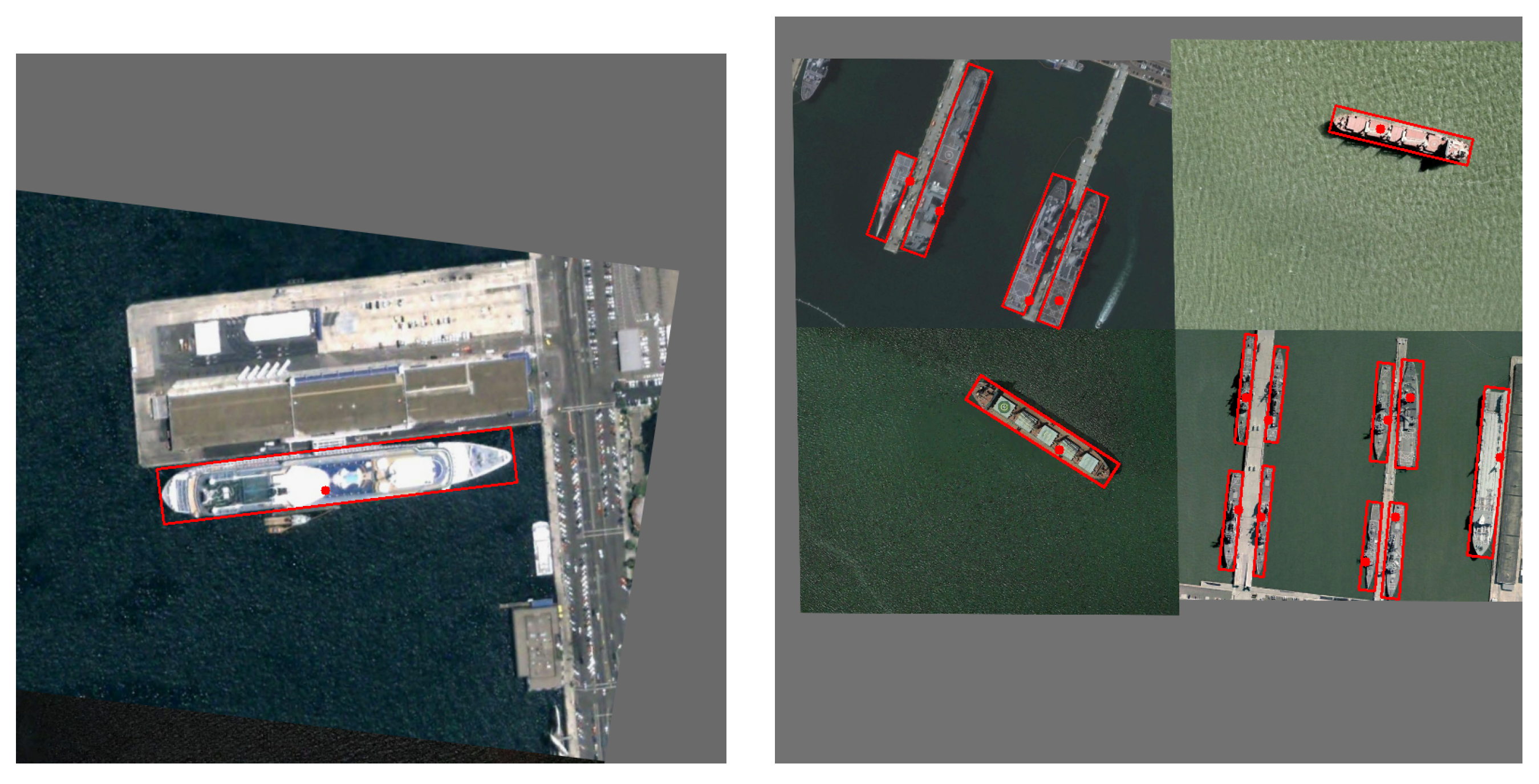
During the experiment, we identify an issue with SimOTA, namely that it assigns an insufficient number of positive samples during the early stages of training. To analyze this issue, we performed a visualization analysis of the number and position of positive samples assigned to each GT during training in Figure 8. In the early stages of training, SimOTA assigns only a small number of positive samples to each GT (in Figure 8, it assigns only one positive sample to each GT). This is because it determines the number of positive samples based on the detection quality, which is poor in early training. The network convergence is slow and unstable due to the lack of positive samples, which has a negative impact on the final detection accuracy.

A straightforward resolution to this issue is increasing the number of positive samples assigned to each object. This helps the model learn object features and location information more effectively, discriminate between objects and backgrounds, and improve accuracy and network convergence. However, an excessive number of positive samples may lead to redundant detection. Therefore, it is necessary to control the ratio of positive and negative samples reasonably to avoid oversampling.

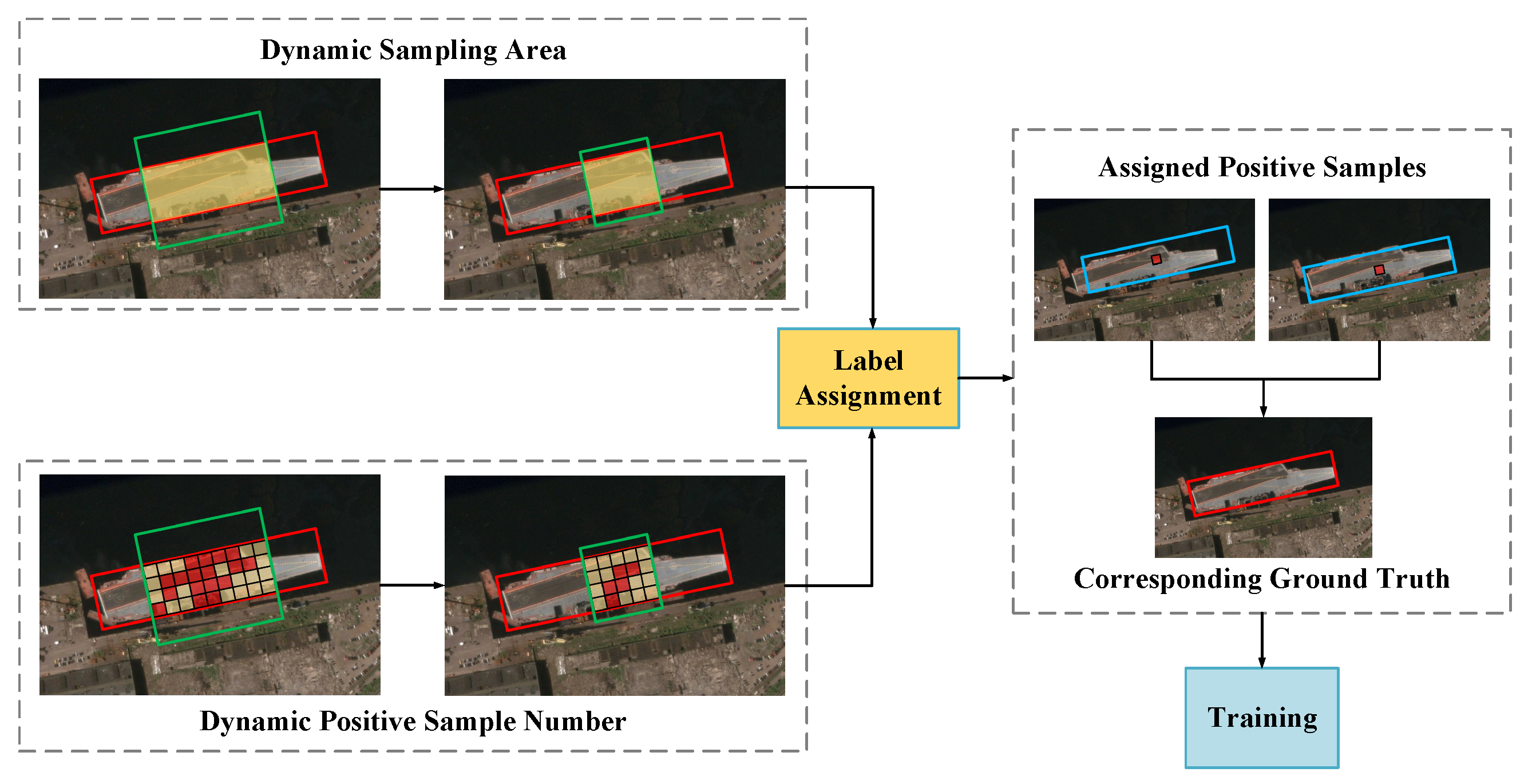
To address the above problem, we propose a label assignment strategy called DynamicOTA, as shown in Figure 9, which consists of two parts:

The first part dynamically adjusts the sampling area. The distance threshold of the sample is calculated as follows:

$$D_{sample}\left(x\right)=2.5-x,$$

(8)

where $D_{sample}\left(x\right)$ is the distance threshold for the sample area. A sample is selected as positive if the distance between the sample center and the GT center is less than the $D_{sample}\left(x\right)$ grid size. x denotes the training process, taking values within the $[0,1]$ range. As shown in Figure 9, the green box represents the region defined by $D_{sample}\left(x\right)$, which gradually shrinks during training. This strategy enables training to focus on high-quality detection results, reducing unnecessary memory and computational overhead and ultimately improving the training efficiency and detection quality.

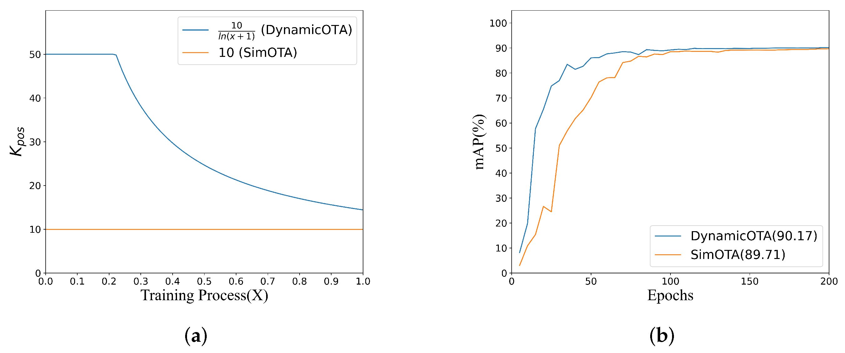
The second part dynamically adjusts the number of positive samples assigned to each GT based on the training process. We adjust the number of positive samples by constructing a decay function as follows:

$$K_{pos}\left(x\right)=min(50,10\ast \frac{1}{ln(x+1)}),$$

(9)

where x represents the training progress, with a value range between $[0,1]$. The number of positive samples $N_{pos}$ assigned to each GT is the sum of the top $K_{pos}\left(x\right)$ IoU values (IoU calculated between the detection boxes and GT boxes). The maximum value of $K_{pos}\left(x\right)$ is 50. Figure 10a shows the function curve, where $K_{pos}$ is set to 10 in SimOTA, while our method dynamically adjusts $K_{pos}$.

Our DynamicOTA algorithm is shown in Algorithm 1. We first calculate the classification and regression cost. Subsequently, we calculate the foreground–background cost based on the sampling area adjusted by $D_{sample}\left(x\right)$. Finally, we assign the $N_{pos}$ samples with the smallest total cost to the corresponding GT as the positive sample.

Algorithm 1 DynamicOTA

Input:

I is the input images. A is the anchor points. G is the GT labels. X is the training process $X\in [0,1]$.

Output:

$\pi *$: Label assignment result.

1: $m\leftarrow \left|G\right|,n\leftarrow \left|A\right|$;

2: $P_{j,cls},P_{j,box},P_{j,score}\leftarrow \mathrm{Forward}\left(I\right)$$(j=1,2,...,n);$

3: Compute classification $Cost$: $c_{cls,ij}\leftarrow \mathrm{BCELoss}(P_{j,cls}\ast P_{j,score},G_{i,cls})$$(i=1,2,...,m);$

4: Compute regression $Cost$: $c_{reg,ij}\leftarrow \mathrm{IoULoss}(P_{j,box},G_{i,box})$;

5: Dynamically adjust the sampling area $A_j^d\leftarrow {\mathrm{D}}_{Sample}(A_j,X)$;

6: Compute foreground-background $Cost$: $c_{fg,ij}\leftarrow (A_j^d,G_{i,box})$;

7: $Cost$ = $c_{cls,ij}+c_{reg,ij}+c_{fg,ij};$

8: $\forall i\in [1,K_{pos}\left(X\right)],p_i\leftarrow$Select the largest $K_{pos}\left(X\right)$ IoU values between $P_{box}$ and $G_{box}$;

9: $N_{pos}\leftarrow {\displaystyle \sum _{i=1}^{K_{pos}\left(X\right)}}{p}_i$;

10: for $g=0\to m$ do

11:   ${\pi }_g^{*}\leftarrow$Select the smallest $N_{pos}$ samples from the $Cos{t}_g$ as the positive samples of $G_g$;

12: end for

13: return $\pi *$.

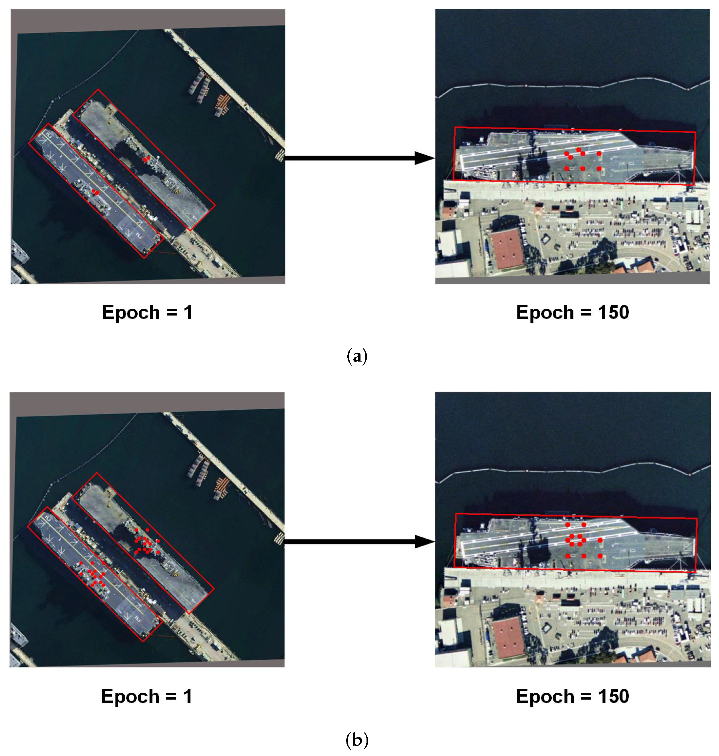
Figure 11 shows a visualization of label assignment during training, where red boxes denote GT boxes and red dots denote positive samples. In the early stages of training, SimOTA assigns very few positive samples to each GT, resulting in slow network convergence. Our DynamicOTA has a more reasonable label assignment process that transitions from dense to sparse. In the early stages of training, DynamicOTA assigns more positive samples, facilitating stable and comprehensive learning and accelerating network convergence. As training progresses, the number of assigned positive samples is adaptively decreased to suppress the redundant detection results, which not only helps to accelerate the convergence process, but also can improve the detection precision by further training with fewer high-quality samples.

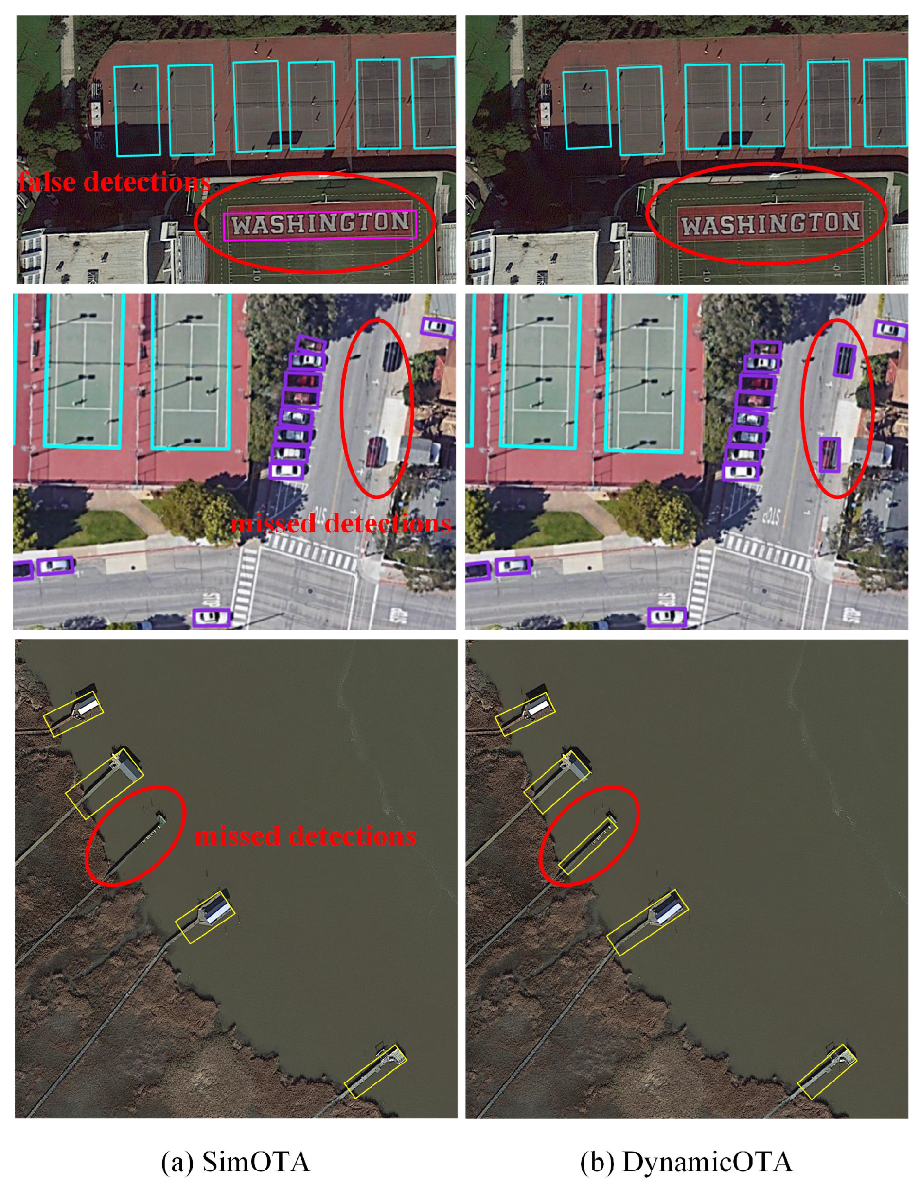
Figure 10b provides an experimental validation of DynamicOTA on the HRSC2016 dataset [37] by comparing it with the original SimOTA. It shows that our method can significantly improve the convergence speed and the final accuracy of the detector.

3.3. Sample Selection Module for End-to-End Oriented Object Detection

The current detector uses one-to-many matching to assign multiple positive samples to a single GT. This approach leads to multiple detection boxes corresponding to a single object during inference, requiring NMS to eliminate duplicate bounding boxes. NMS is a heuristic algorithm in object detection that plays a similar role to that of the anchor. Analogous to anchor-Free detectors, NMS-free detectors have been introduced. DETR [38] uses a transformer structure to fix 100 prediction results and achieves end-to-end detection. DeFCN [39] uses a one-to-one matching strategy and 3D max filtering to achieve NMS-free detection. PSS [40] implements NMS-free detection using a simple convolutional structure.

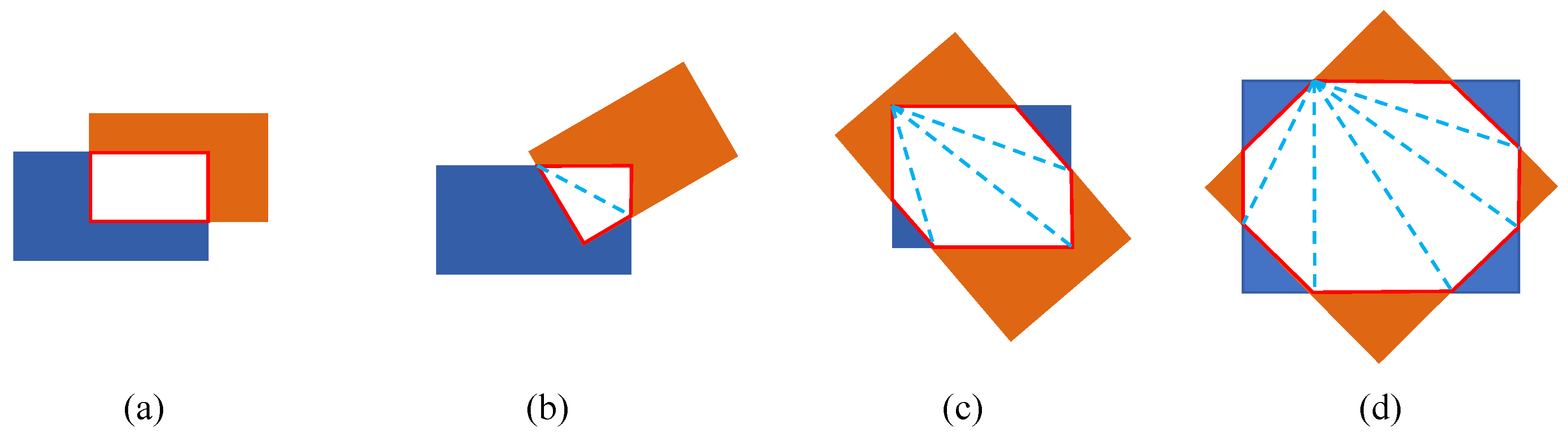
The NMS algorithm needs to calculate the IoU between different detection boxes to eliminate redundant detections. For HBB detection, the calculation of the IoU is relatively simple. However, for OBB detection, the calculation of rotated IoU is complex, requiring consideration of various cases as shown in Figure 12. In addition, post-processing with NMS adds an extra algorithm module that prevents the network from being fully end-to-end. In comparison, the NMS-free method enables end-to-end detection and achieves comparable performance, facilitating network deployment on embedded devices.

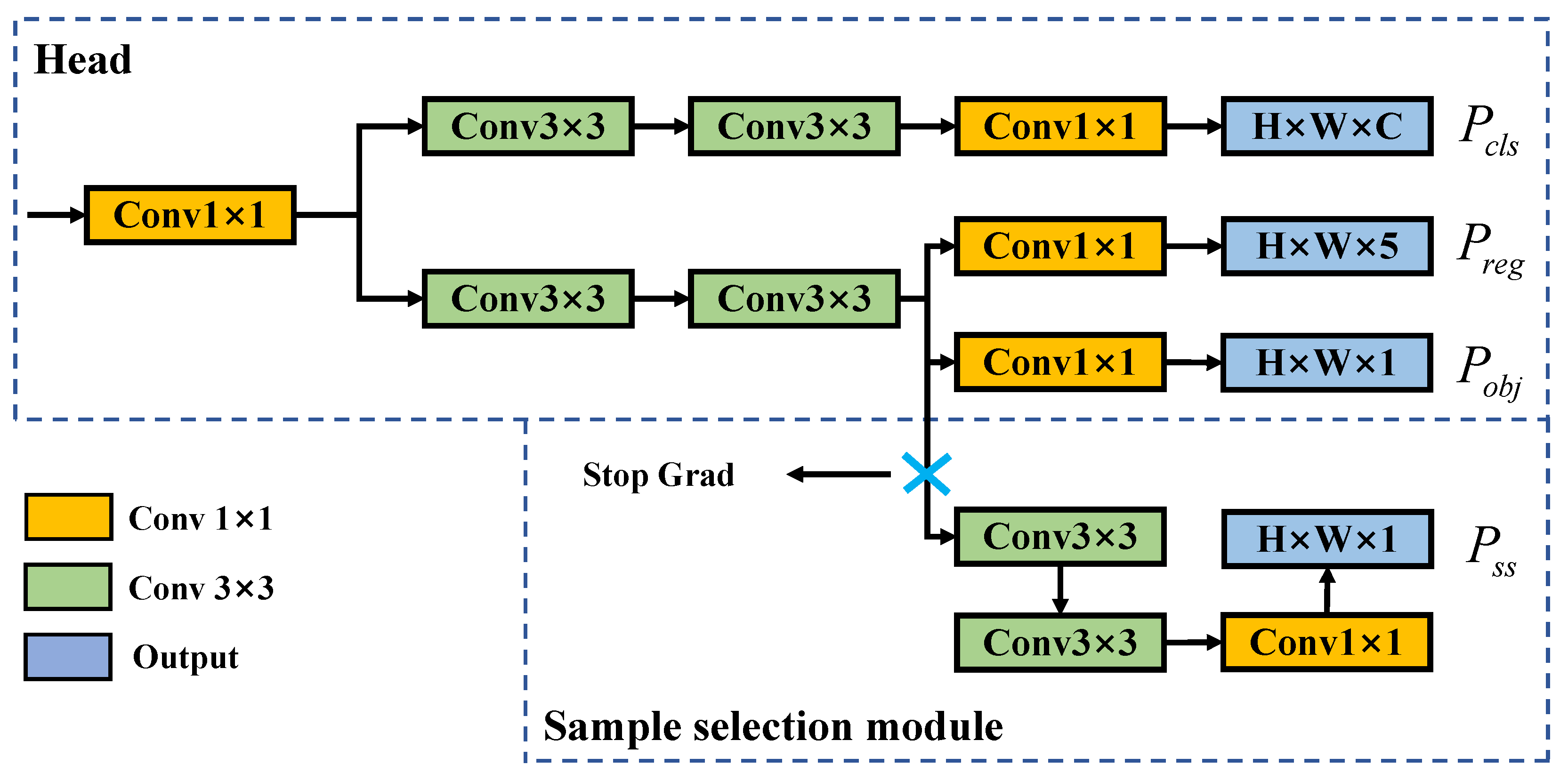
We implement full end-to-end object detection using a convolutional structure to facilitate deployment and engineering applications. We add an SSM to the detection head, as shown in Figure 13. The SSM outputs a map corresponding to each GT box, where the map is 1 at the optimal detection position and 0 at other anchor points. We can remove the redundant detections by multiplying the output map with the detection result, thus eliminating the need for the NMS algorithm.

The SSM consists of two $3\times 3$ convolution layers and one $1\times 1$ convolution layer, as shown in Figure 14. The detection results can be filtered as follows:

$$P_{out}=Sigmoid\left(P_{obj}\right)\ast Sigmoid\left(P_{ss}\right),$$

(10)

in which $Sigmoid(·)$ denotes the sigmoid activation function, $P_{ss}$ is the SSM output, $P_{obj}$ is the confidence output, and $P_{out}\in [0,1]$ is the one-to-one confidence score corresponding to the GT. The $P_{out}$ is the confidence output of the final detection result and does not require NMS processing.

The SSM is trained with the following cross-entropy (CE) loss function:

$$L_{ss}=\frac{CE(Sigmoid\left(P_{ss}\right),G_{ss})}{N_{pos}},$$

(11)

in which $P_{ss}$ denotes the SSM output, indicating the samples that should be selected and those that should be discarded. $G_{ss}$ denotes the map of the GT, with each GT set to 1 at the position with the best detection result and 0 at other positions. $N_{pos}$ is the number of positive samples; it is employed to normalize the calculation of the loss function.

The confidence output calculates losses by considering multiple positive samples for each GT. Conversely, the SSM output calculates losses with only the best positive sample for each GT, establishing a one-to-one matching, which reduces redundant detection boxes. However, this can cause negative samples from the SSM branch to be considered positive by the confidence branch, leading to gradient conflicts during training. To address this issue, PSS [40] adopts a strategy of stopping gradient backpropagation. As shown in Figure 14, we introduce this approach to achieve better performance. Furthermore, we observe that adding the SSM directly to the training results in slower convergence and decreased accuracy. Therefore, we adopte an alternative approach using the model weights trained without the SSM as the pre-trained weights to guide the training process.

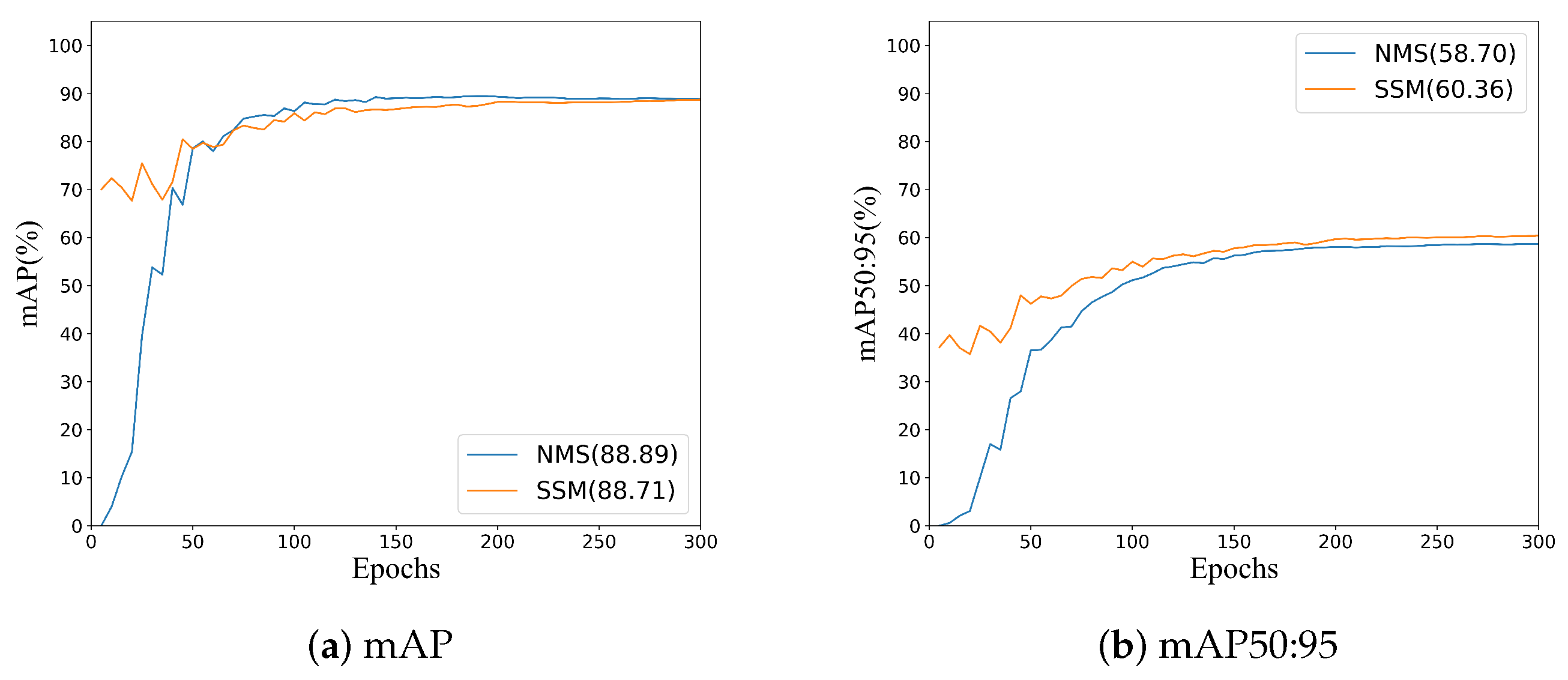
As shown in Figure 15, our method shows comparable performance to that of the NMS method on the mAP (IoU threshold is 0.5) metric and a significant improvement on the mAP50:95 metric, which concerns more the evaluation of higher-precision detection. This demonstrates the advantage of one-to-one matching between GT and the best positive sample in training for high-precision detection. In addition, SSM employs a pure convolutional structure, making it more suitable for network deployment in embedded devices. However, there is a slight decrease in mAP. Therefore, we set the SSM as an optional component. Specifically, when deploying networks on high-performance GPU and preferring to achieve higher detection accuracy in terms of mAP, the network without SSM can be used; when deploying networks on embedded devices, adding SSM to enable NMS-free detection offers deployment benefit and can typically obtain higher localizing precision (in terms of mAP50:95).

4. Experiments

4.1. Datasets and Implementation Details

4.1.1. HRSC2016

HRSC2016 (High-Resolution Remote Sensing Ship Detection Challenge 2016) [37] is a challenging high-resolution ship detection dataset that includes ships of various sizes and shapes, with a total of 1061 images. Image sizes range from 300 × 300 to 1500 × 900. The dataset contains many rotation ships with large aspect ratios. All objects are annotated with OBBs. The entire dataset is divided into train, validation, and test groups containing 436, 181, and 444 images.

We conducted ablation studies and main experiments on HRSC2016. The input resolution for training and testing images was set to 800 × 800. The training was conducted using the SGD optimizer, with a learning rate of 0.05. We trained the model for 200 epochs on RTX 3090 GPU with the batch size set to 8.

4.1.2. DOTA

DOTA [41] is a large public dataset for object detection in aerial images. The image sizes in DOTA range from 800 × 800 to 20,000 × 20,000, containing objects with various scales, orientations, and shapes. It includes 2806 aerial images with a total of 188,282 annotated instances. There are 15 categories in total, including airplanes (PL), baseball diamonds (BD), bridges (BR), ground track fields (GTF), small vehicles (SV), large vehicles (LV), ships (SH), tennis courts (TC), basketball courts (BC), storage tanks (ST), soccer fields (SBF), roundabouts (RA), harbors (HA), swimming pools (SP), and helicopters (HC). The entire dataset is divided into training, validation, and testing sets, with ratios of 1/2, 1/6, and 1/3, respectively.

We note that the images in DOTA are too large; therefore, we cropped the original images into 1024 × 1024 patches with the stride 200 for training and testing. SGD optimizer was used for training, and the learning rate was set to 0.1. We trained the model on RTX 3090 GPU for 200 epochs with the batch size set to 32.

4.2. Ablation Study

4.2.1. Evaluation of the Proposed Modules

We conducted experiments on the HRSC2016 dataset and DOTA dataset to demonstrate the effectiveness of our proposed modules. YOLOX-S was used as the baseline in this paper. All experiments adopted the same data augmentation and training strategies. The experimental results are shown in

Table 1. Effects of the proposed components on HRSC2016 dataset.

Method	Different Variants
RE-Net	×	✓	✓	✓
DynamicOTA	×	×	✓	✓
SSM	×	×	×	✓
mAP 1	88.20	89.82	90.17	89.46
mAP50:95	60.07	68.06	68.48	70.44

¹ mAP (IoU threshold is 0.5). ✓ represents that the corresponding module is used in the method, while × indicates that the corresponding module is not used in the method.

and

Table 2. Effects of the proposed components on DOTA dataset.

Method	Different Variants
RE-Net	×	✓	✓	✓
DynamicOTA	×	×	✓	✓
SSM	×	×	×	✓
mAP	73.85	75.51	76.27	76.15

✓ represents that the corresponding module is used in the method, while × indicates that the corresponding module is not used in the method.

.

The proposed RE-Net significantly improves the detection performance, with accuracies of mAP and mAP50:95 increased by 1.62% and 7.99%, respectively. This indicates that the channel expansion structure can enhance the network’s ability to extract features in different dimensions, thus improving detection performance. When trained with the DynamicOTA, our model further improved mAP by 0.35%, proving its effectiveness. In addition, the NMS-free method achieved an increase of 1.96% in mAP50:95, though there was a slight decrease in mAP.

We further conducted experiments on the DOTA dataset. The image size was resized to 1024 × 1024 using single-scale training and testing. The experimental results are shown in Table 2. With the proposed RE-Net and DynamicOTA, mAP can be increased from 73.85% to 76.27%, and it can also cause a slight decrease in mAP that is ignorable when using SSM for the deployment of NMS-free detection.

4.2.2. Evaluation of Re-Parameterization Channel Expansion Network

To obtain the optimal channel expansion hyperparameters, we conducted experiments as shown in

Table 3. Analysis of RE-Net on HRSC2016 dataset.

Backbone	ELAN	RepExpand	Expand Ratio	mAP	mAP50:95
CSPDarkNet	×	-	-	88.20	60.07
RE-Net	✓	×	-	89.48	64.85
	✓	✓	0.5	89.13	63.81
	✓	✓	1.0	89.56	64.48
	✓	✓	1.5	89.78	66.43
	✓	✓	2.0	89.82	68.06
	✓	✓	2.5	89.59	67.04

✓ represents that the corresponding module is used in the method, while × indicates that the corresponding module is not used in the method.

. The introduction of the ELAN structure improved mAP and mAP50:95 by 1.28% and 4.78%, respectively. As the channel expansion factor increases, the proposed RE-Net obtains better detection performance. The highest performance was achieved when the channel expansion factor E was set to 2.0, with mAP and mAP50:95 reaching 89.82% and 68.06%, respectively. Nevertheless, the performance decreased as the channel expansion factor E increased to 2.5. This suggests that setting a channel expansion factor that is too large does not improve network performance but instead has negative effects. Consequently, we set the channel expansion factor to 2.0.

4.2.3. Evaluation of DynamicOTA

The ablation study on DynamicOTA is shown in

Table 4. Analysis of DynamicOTA on HRSC2016 dataset.

Backbone	DynamicOTA	mAP	mAP50:95
CSPDarkNet	×	88.20	60.07
	✓	89.20	67.50
RE-Net	×	89.82	68.06
	✓	90.17	68.48

✓ represents that the corresponding module is used in the method, while × indicates that the corresponding module is not used in the method.

. DynamicOTA improves accuracy over different backbones. With YOLOX’s CSPDarkNet as the backbone, mAP and mAP50:95 are improved by 1.00% and 7.43%, respectively. With our RE-Net as the backbone, mAP and mAP50:95 are improved by 0.35% and 0.42%, respectively. Experimental results confirm the effectiveness and generalization of DynamicOTA.

Figure 16 further offers the visualization of some detection results. Our detector is sufficiently trained due to improved label assignment, helping to achieve better performance. Compared with SimOTA, our method can obtain better results with fewer false detections (see the first row in Figure 16) and missed detections (see the second and third rows in Figure 16).

4.2.4. Evaluation of Sample Selection Module

Table 5. Analysis of sample selection module on HRSC2016 dataset.

Backbone	Method	Pretrain	Stop Grad	mAP	mAP50:95
CSPDarkNet	NMS	-	-	88.20	60.07
CSPDarkNet	SSM	×	×	80.60	52.45
		✓	×	81.93	55.87
		✓	✓	88.48	66.18
RE-Net	NMS	-	-	89.82	68.68
RE-Net	SSM	✓	✓	89.41	69.29

✓ represents that the corresponding module is used in the method, while × indicates that the corresponding module is not used in the method.

shows the results of ablation study for the NMS-free method on the HRSC2016 dataset. From the results based on CSPDarkNet, it can be seen that the strategies of pre-train and stopping gradient backpropagation are both necessary for the training of SSM. The proposed SSM finally increases mAP by 0.28% and mAP50:95 by 6.11%, proving the superiority of this approach. When using RE-Net as the backbone network, the mAP decreased slightly while the mAP50:95 increased, suggesting that the NMS-free method may suffer a slight mAP degradation as the mAP approaches state-of-the-art condition. In comparison, mAP50:95, which indicates the performance of higher-precision detection, obtained more notable improvement. Since we know that our method with SSM has a very small decrease in mAP but obtains more profit in mAP50:95, in the following experimental comparison with the other detectors, we only use the metric mAP for quantitative comparison as generally performed in the current literature.

4.3. Main Results

4.3.1. Results on HRSC2016

Table 6. Comparisons with other methods on HRSC2016 dataset.

Method	Backbone	Size	mAP
Two-Stage:
RoI Trans. [13]	ResNet101	512 × 800	86.20
GlidingVertex [42]	ResNet101	512 × 800	88.20
DCL [43]	ResNet101	800 × 800	89.46
Oriented R-CNN [17]	ResNet50	800 × 800	90.40
Single-Stage:
RSDet [44]	ResNet152	800 × 800	86.50
BBAVectors [29]	ResNet101	608 × 608	88.60
PIoU [32]	DLA-34	512 × 512	89.20
R${}^3$Det [27]	MobileNetV2	800 × 800	88.71
SLA [45]	ResNet101	768 × 768	89.51
DAL [46]	ResNet101	800 × 800	89.77
FCOSR-S [14]	MobileNetV2	800 × 800	90.08
S${}^2$ANet [12]	ResNet101	800 × 800	90.17
Ours (NMS)	RE-Net	800 × 800	90.17
Ours (SSM)	RE-Net	800 × 800	89.50

shows the performance comparison of different methods on the HRSC2016 dataset. The results with red and blue colors indicate the best and second best results, respectively. Our method without SSM outperforms other compared single-stage methods, with the mAP achieving 90.17%. Our NMS-free method of adding SSM also achieves comparable performance, with mAP achieving 89.50%.

The visualization of some detection results is provided in Figure 17. Our method can accurately detect the ship in complex scenes in aerial images. Even for densely arranged long narrow ships that are difficult to detect, our method still performs well and outputs high-quality detection results (see the first row in Figure 17). Our method still detects objects accurately when the weather and lighting change (see the third row in Figure 17).

4.3.2. Results on DOTA

We conducted performance comparisons with some advanced detectors on the DOTA dataset, and the results are shown in

Table 7. Comparisons with other state-of-the-art methods on DOTA dataset.

Method	Backbone	PL	BD	BR	GTF	SV	LV	SH	TC	BC	ST	SBF	RA	HA	SP	HC	mAP
Anchor-Based (Two-Stage)
RoI Trans. [13]	R101	88.64	78.52	43.44	75.92	68.81	73.68	83.59	90.74	77.27	81.46	58.39	53.54	62.83	58.93	47.67	69.56
CSL [47]	R152	90.25	85.53	54.64	75.31	70.44	73.51	77.62	90.84	86.15	86.69	69.60	68.04	73.83	71.10	68.93	76.17
ReDet [16]	ReR50	88.79	82.64	53.97	74.00	78.13	84.06	88.04	90.89	87.78	85.75	61.76	60.39	75.96	68.07	63.59	76.25
Oriented R-CNN [17]	R101	88.86	83.48	55.27	76.92	74.27	82.10	87.52	90.90	85.56	85.33	65.51	66.82	74.36	70.15	57.28	76.28
Anchor-Based (Single-Stage)
DAL [46]	R101	88.61	79.69	46.27	70.37	65.89	76.10	78.53	90.84	79.98	78.41	58.71	62.02	69.23	71.32	60.65	71.78
SLA [45]	R101	85.23	83.78	48.89	71.65	76.43	76.80	86.83	90.62	88.17	86.88	49.67	66.13	75.34	72.11	64.88	74.89
S${}^2$ANet [12]	R50	89.11	82.84	48.37	71.11	78.11	78.39	87.25	90.83	84.90	85.64	60.36	62.60	65.26	69.13	57.94	74.12
R${}^3$Det [27]	R101	89.80	83.77	48.11	66.77	78.76	83.27	87.84	90.82	85.38	85.51	65.67	62.68	67.53	78.56	72.62	76.47
Anchor-Free (Single-Stage)
PIoU [32]	DLA34	80.90	69.70	24.10	60.20	38.30	64.40	64.80	90.90	77.20	70.40	46.50	37.10	57.10	61.90	64.00	60.50
BBAVectors [29]	R101	88.63	84.06	52.13	69.56	78.26	80.4	88.06	90.87	87.23	86.39	56.11	65.62	67.10	72.08	63.96	75.36
PolarDet [30]	R50	89.73	87.05	45.30	63.32	78.44	76.65	87.13	90.79	80.58	85.89	60.97	67.94	68.20	74.63	68.67	75.02
FCOSR [14]	MobileNetv2	89.09	80.58	44.04	73.33	79.07	76.54	87.28	90.88	84.89	85.37	55.95	64.56	66.92	76.96	55.32	74.05
Oriented RepPoints [31]	R50	87.02	83.17	54.13	71.16	80.18	78.40	87.28	90.90	85.97	86.25	59.90	70.49	73.53	72.27	58.97	75.97
Ours (NMS)	RE-Net	88.88	83.99	51.20	71.77	81.33	78.15	88.58	90.88	87.60	86.51	61.34	62.35	76.36	73.51	61.69	76.28
Ours (SSM)	RE-Net	87.67	83.40	53.37	69.29	81.22	84.00	88.73	90.86	87.30	87.00	57.14	66.45	76.44	71.28	58.13	76.15

. The results with red colors indicate the best results for the corresponding detector category. The image size was resized to 1024 × 1024, using single-scale training and testing. Our NMS and NMS-free methods achieved the mAP of 76.27% and 76.15%, respectively, which are the highest and second highest values among the compared anchor-free detectors.

Figure 18 shows visualizations of the detection results obtained by our detector in comparison with state-of-the-art detectors. Our detector performs better in detecting different categories, such as vehicles, helicopters, harbours, and ships. Moreover, our anchor-free single-stage detector has a more streamlined architecture and fewer parameters compared with anchor-based two-stage detectors like Oriented R-CNN [17] and single-stage detectors like S${}^2$ANet [12].

Figure 19 shows some visualization of the detection results. It can be observed that the objects in the DOTA dataset vary greatly in scale, and many objects are densely arranged. Detecting densely arranged small objects, such as small vehicles and ships, is challenging in aerial images. Our detector achieves excellent performance in dense object detection without missed detection (see the first row of Figure 19). In addition, our detector does not have repeated detection for large objects and achieves accurate detection (see the second row of Figure 19). From the UAV aerial perspective, objects usually have complex backgrounds, while our detector accurately detects the objects in the image (see the third row of Figure 19).

4.3.3. Results of Deployment

We conducted a re-parameterization experiment on the DOTA dataset using a 1 × NVIDIA GTX 1080Ti and 1024 × 1024 input image size. Comparison of the results before and after re-parameterization are shown in

Table 8. Inference time, parameters and GFLOPs before and after re-parameterization.

Re-Parameterization	Parameters	GFLOPs	Inference Time	mAP
×	18.07 M	193.67 G	24.9 ms	76.15
✓	16.95 M	188.40 G	22.3 ms	76.15

✓ represents that the corresponding module is used in the method, while × indicates that the corresponding module is not used in the method.

. After the re-parameterization, the model parameters, computation load, and inference time are reduced. Meanwhile, the detection accuracy remains the same as that before the transformation.

We tested the inference speed of several compared algorithms as shown in

Table 9. Inference time and mAP on DOTA dataset for different detection models.

Method	S2ANet [12]	ReDet [16]	R${}^3$Det [27]	Oriented RepPoints [31]	Ours
Inference Time	81.5 ms	106.6 ms	102.6 ms	75.3 ms	22.3 ms
mAP	74.12	76.25	76.47	75.97	76.15

. We used DOTA as the test dataset with the image size of 1024 × 1024 and the batch size set to one. Our detector achieved a competitive mAP, while the inference speed was much faster than that of the other detectors.

In addition, a statistical analysis with the Friedman test and post hoc Nemenyi test [48] was performed on the detection accuracy scores of these representative detection algorithms on different datasets. The assumption that two algorithms perform the same in accuracy can be rejected when the p-value obtained by the test is smaller than 0.05. Through the Friedman test, we obtained p = 0.025, indicating that there is a significant difference in performance among the methods of S${}^2$ANet, ReDet, R${}^3$Det, Oriented RepPoints and Ours. The post hoc Nemenyi test further provided the p-values for the pairwise comparisons. More specifically, we obtained p = 0.021 for the comparing pair Ours-S${}^2$ANet, indicating statistically significant difference in performance between our algorithm and S${}^2$ANet (which can also be seen from the mAP in Table 9). As for the methods of ReDet, R${}^3$Det, Oriented RepPoints that have relatively high accuracy, the Nemenyi test shows that there is no significant statistical difference between them and Ours (p = 0.900, 0.739, 0.900 for Ours-ReDet, Ours-R${}^3$Det and Ours-Oriented RepPoints, respectively). However, as shown in Table 9, our method consumes significantly lower inference time compared with them, revealing its good overall performance in detection accuracy and speed.

Next, we deployed our detector on the NVIDIA Jetson Xavier NX embedded device. The inference batch size was set to one, the experimental dataset was HRSC2016, and the input images were resized to 800 × 800. We performed L1 weight channel pruning to accelerate the network inference speed further, as shown in

Table 10. Deployment results on NVIDIA Jetson Xavier NX.

Method	Parameters	GFLOPs	Inference Speed	mAP
Baseline	16.95 M	114.84 G	28.40 FPS	89.50
30% Pruning	9.40 M	65.86 G	35.07 FPS	89.39
40% Pruning	7.33 M	52.28 G	37.93 FPS	89.33
50% Pruning	5.58 M	40.50 G	56.46 FPS	88.89

. Our detector achieved an inference speed of 28.40 FPS. After channel pruning, the inference speed was improved to 56.46 FPS. Moreover, our detector was easy to deploy on various embedded devices, such as FPGAs and ARMs, as it does not require NMS post-processing.

5. Conclusions

In this study, we analyzed the limitations of current oriented object detection methods, which frequently employ complex network structures, exhibit slow inference speeds, and present deployment challenges. We proposed a fast and easy-to-deploy oriented detector for UAV aerial images. First, we designed a RE-Net that enhances the feature representation capabilities of the network and can better address the challenges of UAV aerial object detection. During inference, RE-Net can be equivalently converted to a more streamlined structure, reducing the parameters and computational load. To further improve the detection performance in aerial images, we propose DynamicOTA, which facilitates high-accuracy detection in UAV aerial images. Dynamic label assignment effectively addresses the imbalance between positive and negative samples and solves the problem of insufficient positive samples in the early stages of training, thereby improving the training speed, stability, and detection accuracy. In addition, we explored NMS-free techniques and introduced an SSM to facilitate the deployment of our detector on embedding devices. Extensive experiments on aerial image datasets demonstrate the superiority of our method. We achieved the mAP of 76.27% and 76.15% on the DOTA dataset and 90.17% and 89.50% on the HRSC2016 dataset using the NMS and NMS-free methods, respectively, outperforming many advanced oriented detectors. We deployed our NMS-free detector on NVIDIA Jetson Xavier NX and achieved 28.40 FPS at an 800 × 800 image size. In the future, we will further study ways to combine label assignment strategies to guide the training of the NMS-free detector to achieve better end-to-end object detection.

References

1. Ge, Z.; Liu, S.; Wang, F.; Li, Z.; Sun, J. Yolox: Exceeding yolo series in 2021. arXiv 2021, arXiv:2107.08430. [Google Scholar]
2. Redmon, J.; Farhadi, A. Yolov3: An incremental improvement. arXiv 2018, arXiv:1804.02767. [Google Scholar]
3. Bochkovskiy, A.; Wang, C.Y.; Liao, H.Y.M. Yolov4: Optimal speed and accuracy of object detection. arXiv 2020, arXiv:2004.10934. [Google Scholar]
4. Wang, C.Y.; Bochkovskiy, A.; Liao, H.Y.M. YOLOv7: Trainable bag-of-freebies sets new state-of-the-art for real-time object detectors. arXiv 2022, arXiv:2207.02696. [Google Scholar]
5. Girshick, R.; Donahue, J.; Darrell, T.; Malik, J. Region-based convolutional networks for accurate object detection and segmentation. IEEE Trans. Pattern Anal. Mach. Intell. 2015, 38, 142–158. [Google Scholar] [CrossRef]
6. Girshick, R. Fast r-cnn. In Proceedings of the IEEE International Conference on Computer Vision, Santiago, Chile, 7–13 December 2015; pp. 1440–1448. [Google Scholar]
7. Ren, S.; He, K.; Girshick, R.; Sun, J. Faster r-cnn: Towards real-time object detection with region proposal networks. Adv. Neural Inf. Process. Syst. 2015, 28, 1440–1448. [Google Scholar] [CrossRef]
8. Cai, Z.; Vasconcelos, N. Cascade r-cnn: Delving into high quality object detection. In Proceedings of the IEEE Conference on Computer Vision and Pattern Recognition, Salt Lake City, UT, USA, 18–23 June 2018; pp. 6154–6162. [Google Scholar]
9. Lin, T.Y.; Goyal, P.; Girshick, R.; He, K.; Dollár, P. Focal loss for dense object detection. In Proceedings of the IEEE International Conference on Computer Vision, Venice, Italy, 22–29 October 2017; pp. 2980–2988. [Google Scholar]
10. Tian, Z.; Shen, C.; Chen, H.; He, T. Fcos: Fully convolutional one-stage object detection. In Proceedings of the IEEE/CVF International Conference on Computer Vision, Seoul, Republic of Korea, 27 October–2 November 2019; pp. 9627–9636. [Google Scholar]
11. Duan, K.; Bai, S.; Xie, L.; Qi, H.; Huang, Q.; Tian, Q. Centernet: Keypoint triplets for object detection. In Proceedings of the IEEE/CVF International Conference on Computer Vision, Seoul, Republic of Korea, 27 October–2 November 2019; pp. 6569–6578. [Google Scholar]
12. Han, J.; Ding, J.; Li, J.; Xia, G.S. Align deep features for oriented object detection. IEEE Trans. Geosci. Remote Sens. 2021, 60, 5602511. [Google Scholar] [CrossRef]
13. Ding, J.; Xue, N.; Long, Y.; Xia, G.S.; Lu, Q. Learning roi transformer for oriented object detection in aerial images. In Proceedings of the IEEE/CVF Conference on Computer Vision and Pattern Recognition, Long Beach, CA, USA, 15–20 June 2019; pp. 2849–2858. [Google Scholar]
14. Li, Z.; Hou, B.; Wu, Z.; Jiao, L.; Ren, B.; Yang, C. Fcosr: A simple anchor-free rotated detector for aerial object detection. arXiv 2021, arXiv:2111.10780. [Google Scholar]
15. Ming, Q.; Miao, L.; Zhou, Z.; Dong, Y. CFC-Net: A critical feature capturing network for arbitrary-oriented object detection in remote-sensing images. IEEE Trans. Geosci. Remote Sens. 2021, 60, 5605814. [Google Scholar] [CrossRef]
16. Han, J.; Ding, J.; Xue, N.; Xia, G.S. Redet: A rotation-equivariant detector for aerial object detection. In Proceedings of the IEEE/CVF Conference on Computer Vision and Pattern Recognition, Virtual, 19–25 June 2021; pp. 2786–2795. [Google Scholar]
17. Xie, X.; Cheng, G.; Wang, J.; Yao, X.; Han, J. Oriented R-CNN for object detection. In Proceedings of the IEEE/CVF International Conference on Computer Vision, Montreal, BC, Canada, 11–17 October 2021; pp. 3520–3529. [Google Scholar]
18. Xie, X.; Li, L.; An, Z.; Lu, G.; Zhou, Z. Small Ship Detection Based on Hybrid Anchor Structure and Feature Super-Resolution. Remote Sens. 2022, 14, 3530. [Google Scholar] [CrossRef]
19. Xiao, X.; Zhou, Z.; Wang, B.; Li, L.; Miao, L. Ship detection under complex backgrounds based on accurate rotated anchor boxes from paired semantic segmentation. Remote Sens. 2019, 11, 2506. [Google Scholar] [CrossRef]
20. Li, L.; Zhou, Z.; Wang, B.; Miao, L.; An, Z.; Xiao, X. Domain adaptive ship detection in optical remote sensing images. Remote Sens. 2021, 13, 3168. [Google Scholar] [CrossRef]
21. Li, L.; Zhou, Z.; Wang, B.; Miao, L.; Zong, H. A novel CNN-based method for accurate ship detection in HR optical remote sensing images via rotated bounding box. IEEE Trans. Geosci. Remote Sens. 2020, 59, 686–699. [Google Scholar] [CrossRef]
22. Ming, Q.; Miao, L.; Zhou, Z.; Song, J.; Dong, Y.; Yang, X. Task interleaving and orientation estimation for high-precision oriented object detection in aerial images. ISPRS J. Photogramm. Remote Sens. 2023, 196, 241–255. [Google Scholar] [CrossRef]
23. Dai, J.; Li, Y.; He, K.; Sun, J. R-fcn: Object detection via region-based fully convolutional networks. Adv. Neural Inf. Process. Syst. 2016, 29, 379–387. [Google Scholar]
24. Liu, W.; Anguelov, D.; Erhan, D.; Szegedy, C.; Reed, S.; Fu, C.Y.; Berg, A.C. Ssd: Single shot multibox detector. In Proceedings of the Computer Vision–ECCV 2016: 14th European Conference, Amsterdam, The Netherlands, 11–14 October 2016; Proceedings, Part I 14. Springer: Berlin/Heidelberg, Germany, 2016; pp. 21–37. [Google Scholar]
25. Ma, J.; Shao, W.; Ye, H.; Wang, L.; Wang, H.; Zheng, Y.; Xue, X. Arbitrary-oriented scene text detection via rotation proposals. IEEE Trans. Multimed. 2018, 20, 3111–3122. [Google Scholar] [CrossRef]
26. Liu, L.; Pan, Z.; Lei, B. Learning a rotation invariant detector with rotatable bounding box. arXiv 2017, arXiv:1711.09405. [Google Scholar]
27. Yang, X.; Yan, J.; Feng, Z.; He, T. R3det: Refined single-stage detector with feature refinement for rotating object. In Proceedings of the AAAI Conference on Artificial Intelligence, Online, 2–9 February 2021; Volume 35, pp. 3163–3171. [Google Scholar]
28. Wei, H.; Zhang, Y.; Chang, Z.; Li, H.; Wang, H.; Sun, X. Oriented objects as pairs of middle lines. ISPRS J. Photogramm. Remote Sens. 2020, 169, 268–279. [Google Scholar] [CrossRef]
29. Yi, J.; Wu, P.; Liu, B.; Huang, Q.; Qu, H.; Metaxas, D. Oriented object detection in aerial images with box boundary-aware vectors. In Proceedings of the IEEE/CVF Winter Conference on Applications of Computer Vision, Waikoloa, HI, USA, 3–8 January 2021; pp. 2150–2159. [Google Scholar]
30. Zhao, P.; Qu, Z.; Bu, Y.; Tan, W.; Guan, Q. Polardet: A fast, more precise detector for rotated target in aerial images. Int. J. Remote Sens. 2021, 42, 5831–5861. [Google Scholar] [CrossRef]
31. Li, W.; Chen, Y.; Hu, K.; Zhu, J. Oriented reppoints for aerial object detection. In Proceedings of the IEEE/CVF Conference on Computer Vision and Pattern Recognition, New Orleans, LA, USA, 18–24 June 2022; pp. 1829–1838. [Google Scholar]
32. Chen, Z.; Chen, K.; Lin, W.; See, J.; Yu, H.; Ke, Y.; Yang, C. Piou loss: Towards accurate oriented object detection in complex environments. In Proceedings of the Computer Vision-ECCV 2020: 16th European Conference, Glasgow, UK, 23–28 August 2020; Proceedings, Part V 16. Springer: Berlin/Heidelberg, Germany, 2020; pp. 195–211. [Google Scholar]
33. Ding, X.; Zhang, X.; Ma, N.; Han, J.; Ding, G.; Sun, J. Repvgg: Making vgg-style convnets great again. In Proceedings of the IEEE/CVF Conference on Computer Vision and Pattern Recognition, Nashville, TN, USA, 19–25 June 2021; pp. 13733–13742. [Google Scholar]
34. Guo, S.; Alvarez, J.M.; Salzmann, M. Expandnets: Linear over-parameterization to train compact convolutional networks. Adv. Neural Inf. Process. Syst. 2020, 33, 1298–1310. [Google Scholar]
35. Sandler, M.; Howard, A.; Zhu, M.; Zhmoginov, A.; Chen, L.C. Mobilenetv2: Inverted residuals and linear bottlenecks. In Proceedings of the IEEE Conference on Computer Vision and Pattern Recognition, Salt Lake City, UT, USA, 18–22 June 2018; pp. 4510–4520. [Google Scholar]
36. Ge, Z.; Liu, S.; Li, Z.; Yoshie, O.; Sun, J. Ota: Optimal transport assignment for object detection. In Proceedings of the IEEE/CVF Conference on Computer Vision and Pattern Recognition, Nashville, TN, USA, 19–25 June 2021; pp. 303–312. [Google Scholar]
37. Liu, Z.; Yuan, L.; Weng, L.; Yang, Y. A high resolution optical satellite image dataset for ship recognition and some new baselines. In Proceedings of the ICPRAM, Porto, Portugal, 24–26 February 2017; pp. 324–331. [Google Scholar]
38. Carion, N.; Massa, F.; Synnaeve, G.; Usunier, N.; Kirillov, A.; Zagoruyko, S. End-to-end object detection with transformers. In Proceedings of the Computer Vision-ECCV 2020: 16th European Conference, Glasgow, UK, 23–28 August 2020; Proceedings, Part I 16. Springer: Berlin/Heidelberg, Germany, 2020; pp. 213–229. [Google Scholar]
39. Wang, J.; Song, L.; Li, Z.; Sun, H.; Sun, J.; Zheng, N. End-to-end object detection with fully convolutional network. In Proceedings of the IEEE/CVF Conference on Computer Vision and Pattern Recognition, Nashville, TN, USA, 19–25 June 2021; pp. 15849–15858. [Google Scholar]
40. Zhou, Q.; Yu, C. Object detection made simpler by eliminating heuristic NMS. IEEE Trans. Multimed. 2023, 1–10. [Google Scholar] [CrossRef]
41. Xia, G.S.; Bai, X.; Ding, J.; Zhu, Z.; Belongie, S.; Luo, J.; Datcu, M.; Pelillo, M.; Zhang, L. DOTA: A large-scale dataset for object detection in aerial images. In Proceedings of the IEEE Conference on Computer Vision and Pattern Recognition, Salt Lake City, UT, USA, 18–22 June 2018; pp. 3974–3983. [Google Scholar]
42. Xu, Y.; Fu, M.; Wang, Q.; Wang, Y.; Chen, K.; Xia, G.S.; Bai, X. Gliding vertex on the horizontal bounding box for multi-oriented object detection. IEEE Trans. Pattern Anal. Mach. Intell. 2020, 43, 1452–1459. [Google Scholar] [CrossRef] [PubMed]
43. Yang, X.; Hou, L.; Zhou, Y.; Wang, W.; Yan, J. Dense label encoding for boundary discontinuity free rotation detection. In Proceedings of the IEEE/CVF Conference on Computer Vision and Pattern Recognition, Nashville, TN, USA, 19–25 June 2021; pp. 15819–15829. [Google Scholar]
44. Qian, W.; Yang, X.; Peng, S.; Yan, J.; Guo, Y. Learning modulated loss for rotated object detection. In Proceedings of the AAAI Conference on Artificial Intelligence, Online, 2–9 February 2021; Volume 35, pp. 2458–2466. [Google Scholar]
45. Ming, Q.; Miao, L.; Zhou, Z.; Song, J.; Yang, X. Sparse label assignment for oriented object detection in aerial images. Remote Sens. 2021, 13, 2664. [Google Scholar] [CrossRef]
46. Ming, Q.; Zhou, Z.; Miao, L.; Zhang, H.; Li, L. Dynamic anchor learning for arbitrary-oriented object detection. In Proceedings of the AAAI Conference on Artificial Intelligence, Online, 2–9 February 2021; Volume 35, pp. 2355–2363. [Google Scholar]
47. Yang, X.; Yan, J. Arbitrary-oriented object detection with circular smooth label. In Proceedings of the Computer Vision-ECCV 2020: 16th European Conference, Glasgow, UK, 23–28 August 2020; Proceedings, Part VIII 16. Springer: Berlin/Heidelberg, Germany, 2020; pp. 677–694. [Google Scholar]
48. Trawiński, B.; Smętek, M.; Telec, Z.; Lasota, T. Nonparametric statistical analysis for multiple comparison of machine learning regression algorithms. Int. J. Appl. Math. Comput. Sci. 2012, 22, 867–881. [Google Scholar] [CrossRef]
Figure 1. Structures of current oriented object detection methods, including (a) AlignConv in S 2 ANet and (b) RoI transformer.
Remotesensing 15 05079 g001
Figure 2. The overall framework of our model. The black line represents the inference process, and the blue line represents the training process. We introduce RE-Net to enhance feature extraction capabilities and incorporate SSM for NMS-free object detection. Additionally, we present the DynamicOTA label assignment strategy to improve network performance in training.
Remotesensing 15 05079 g002
Figure 3. The framework of RepExpand Block.
Remotesensing 15 05079 g003
Figure 4. Structures of Expand Unit.
Remotesensing 15 05079 g004
Figure 5. Transformation of structural re-parameterization.
Remotesensing 15 05079 g005
Figure 6. Matrix form of the convolution process (C = 1).
Remotesensing 15 05079 g006
Figure 7. Structures of ELAN.
Remotesensing 15 05079 g007
Figure 8. Positive sample assignment for SimOTA in early training (the red boxes denote GT boxes, and the red dots represent positive samples). SimOTA assigns only a small number of positive samples to each object at the beginning of training, which makes the network convergence slow and unstable.
Remotesensing 15 05079 g008
Figure 9. The framework of DynamicOTA. DynamicOTA dynamically adjusts the sampling area and the number of positive samples to obtain better label assignment results.
Remotesensing 15 05079 g009
Figure 10. Display of decay function and comparison between DynamicOTA and SimOTA. (a) Decay function curve, (b) comparisons of label assignment strategy on HRSC2016.
Remotesensing 15 05079 g010
Figure 11. Comparison of different label assignment strategies: (a) SimOTA and (b) DynamicOTA. SimOTA assigns only very few positive samples at the beginning of training, while DynamicOTA can assign much more positive samples.
Remotesensing 15 05079 g011
Figure 12. Display of IoU and RIoU calculation. (a) IoU calculation in HBB. (bd) RIoU calculation in OBB [25].
Remotesensing 15 05079 g012
Figure 13. NMS-free object detection based on SSM. The SSM outputs a one-to-one matching map. By performing element-wise multiplication between this map and the detection results, we can achieve NMS-free detection.
Remotesensing 15 05079 g013
Figure 14. Structure of sample selection module.
Remotesensing 15 05079 g014
Figure 15. Comparison of the performance of NMS-free method and base method on the HRSC2016.
Remotesensing 15 05079 g015
Figure 16. Detection results of models trained with different label assignment strategies.
Remotesensing 15 05079 g016
Figure 17. Visualization of some detection results on HRSC2016 dataset.
Remotesensing 15 05079 g017
Figure 18. Visualization of some results of different detectors on DOTA dataset. The red circles indicate the differences among the results of the three detectors.
Remotesensing 15 05079 g018
Figure 19. Visualization of some detection results on DOTA dataset.
Remotesensing 15 05079 g019