Article

Volume Estimation of Stem Segments Based on a Tetrahedron Model Using Terrestrial Laser Scanning Data

1
School of Computer and Information Technology, Xinyang Normal University, Xinyang 464000, China
2
Henan Engineering Research Center of Internet of Things and Smart Security, Xinyang 464000, China
3
Henan Dabieshan National Field Observation and Research Station of Forest Ecosystem, Zhengzhou 450046, China
4
Xinyang Academy of Ecological Research, Xinyang 464000, China
5
Institute of Forest Resources Information Techniques, Chinese Academy of Forestry, Beijing 100091, China
6
School of Mathematics and Statistics, Xinyang Normal University, Xinyang 464000, China
*
Author to whom correspondence should be addressed.
Remote Sens. 2023, 15(20), 5060; https://doi.org/10.3390/rs15205060
Submission received: 12 September 2023 / Revised: 15 October 2023 / Accepted: 20 October 2023 / Published: 21 October 2023
(This article belongs to the Special Issue 3D Point Clouds in Forest Remote Sensing III)

Abstract

:
Stem volume is a very important parameter in forestry inventory and carbon storage. The stem volume estimated by most existing methods deviates from its true value because the irregularity of the stem is usually overlooked. In this study, we propose a stem segment volume estimation based on the tetrahedron model using TLS data. First, the initial stem segment surface model, including the lower, upper, and outer triangular surface models, was gradually reconstructed. Next, the outer surface model was subdivided based on the edge subdivision. Then, a closed triangular surface model without self-intersection was obtained. Afterward, a tetrahedron model of the stem segment was generated using TetGen software (Version 1.6.0) for the triangular surface model. Finally, the stem segment volume was calculated by summing the volumes of all the tetrahedrons in the tetrahedron model. An experiment with 76 stem segments from different tree species with different parameters showed that the reconstructed stem segment surface model effectively reflected the geometrical features of the stem segment surface. Compared to the volume based on the simulated sectional measurement, the MAPE of the volume based on the tetrahedron model was 2.12%. The results demonstrated the validity of the presented method for stem surface reconstruction and stem volume estimation, and the volume based on the tetrahedron model was closer to the true value than that based on the sectional measurement.

1. Introduction

Stem volume, which is closely related to tree biomass and carbon stock, is one of the most important forest features of forest inventory and carbon storage [1,2,3]. Accurate calculation of stem volume is the basis for reliable estimation of stand volume, forest biomass, and carbon storage [2,4].
Stem volume calculations are traditionally divided into two types, destructive (felled trees) and nondestructive (standing trees). For felled trees, stem volume can be calculated using sectional measurements [5]. The stem is subdivided into several short sections, and each stem section is regard as a regular geometrical shape, such as a cylinder or a truncated cone. Stem volume is obtained by summing the volume of all stem sections. To improve accuracy, researchers have proposed various calculation methods for sectional volume, such as Smalian’s formula and Newton’s formula [5,6,7]. For standing trees, the stem volume is usually calculated by the empirical volume formula, which provides a simple way to estimate stem volume based on diameter at breast height and tree height. However, the volume formula was developed based on the stem volume calculated from the sectional measurement of several felled trees of the same species. Ref. [8] found that a minimum of 29 and 81 sample trees were required to develop accurate tree volume allometric estimation models for each species and for all species in the Amazonian Forest, respectively. The destructive approach is time-consuming, laborious, and requires strict and serious fieldwork regulations. Meanwhile, the assumption that the section is a regular shape is the basis for sectional measurement. However, the irregularity of the stem is reflected not only in the shape along the stem, but also in the shape of the stem cross-section. This may result in bias if the stem volume is calculated based on the traditional sectional measurement [7].
In recent years, terrestrial laser scanning (TLS) has provided a measurement technique capable of measuring at the level of millimeters, which is beyond the precision of traditional measurement tools [4,9]. Ref. [10] demonstrated that TLS-based approaches can provide stem diameters at breast height and stem curves that are close to the accuracy requirements of national forest inventories. Ref. [11] argued that TLS will play a critical role in understanding fundamental forestry ecological questions. Several studies have demonstrated the advantage of TLS in successfully retrieving tree attributes, including tree location [12,13], stem diameter [14,15,16], tree crown width [17], and other forest parameters [18,19]. Many algorithms have been developed to estimate stem volume from TLS data, which can be roughly divided into four categories. (a) Empirical volume formula: The stem (tree) volume is estimated using the existing empirical volume formula after retrieving stem diameter and stem height from TLS data. Ref. [20] compared the accuracy of different stem diameter retrieval methods to estimate stem volume from TLS data. The results showed that stem volume estimation using the random sample consensus and convex hull methods was more accurate than that using circle fitting. Ref. [21] retrieved stem diameter by circle fitting every 10 cm along the stem, and used Huber’s formula to estimate stem volume. (b) Quantitative structure modeling (QSM): The stem (tree) is reconstructed as a series of smooth cylinders using the QSM method, and the stem (tree) volume is estimated based on reconstructed cylinders. Refs. [1,22,23,24] used treeQSM [25] to reconstruct a tree and estimate the tree volume using TLS data. (c) Regular geometry model: Ref. [2] estimated the stem volume of Euphrates poplar (Populus euphratica) by a definite integration using a stem diameter retrieved by a Hough transform at every 10 cm along the stem from TLS, and established a stem volume regression model represented by DBH, height, and basal area. Ref. [3] proposed an unwrapping method combined with cylinder fitting, voxelization, and digital elevation models to estimate the volume of standing trees. Ref. [26] represented a tree as a set of closed and complete convex polyhedras after fitting a series of cylinders to approximate the geometry of tree stems and branches, and estimated volume using the Smalian’s formula after stem diameter retrieval. (d) Irregularity geometry model: Ref. [27] separated the point cloud of buttresses with complex structures in continuous thin layers, and outlined a nonconvex polygon manually in ArcGIS (Version 10) software after projecting the layer to a plane. Then, the basal area was calculated based on the nonconvex polygon, and the volume of buttresses was estimated using Smalian’s formula. Refs. [28,29] adopted a voxel-based bounding box method to estimate the volume of trees, stems, and branches. The irregularity in the shape along the stem was considered in the above studies, such as using a flexible cylinder model and retrieving stem diameter at every 10 cm. However, the irregularity of the stem cross-section was overlooked by most of the above methods.
Stem volume cannot be directly measured with conventional tools [1,20]. TLS provides the potential to accurately and directly estimate stem volume as the stem surface geometrical feature is contained in the stem point cloud scanned by TLS [3]. The defects of tree point clouds scanned by TLS at a plot level, such as uneven density and missing data, are difficult to control and avoid [30], and the quality of tree point clouds will affect the precision of retrieved tree parameters. Like the problem of stem diameter retrieval in [16], the problem of stem volume estimation can be divided into two steps: data collection and preprocessing, and numerical calculation. In this study, we focused on the numerical calculation of stem volume estimation considering the irregularity of the stem. Traditionally, the stem has been divided into several stem segments in stem volume estimation, and the accuracy of the stem volume estimation is equivalent to that of the volume estimation of the stem segment. Therefore, we assessed stem segments below the middle of the stem with a given length in this study. The specific objectives of the study as follows: (1) to construct a close and disjoint triangular surface model of a stem segment, (2) to construct a tetrahedral solid geometry model of the stem segment based on the triangular surface model, and to estimate the volume of the stem segment, and (3) to compare the accuracy of volume estimation between the tetrahedron model and the traditional sectional measurement.

2. Materials and Methods

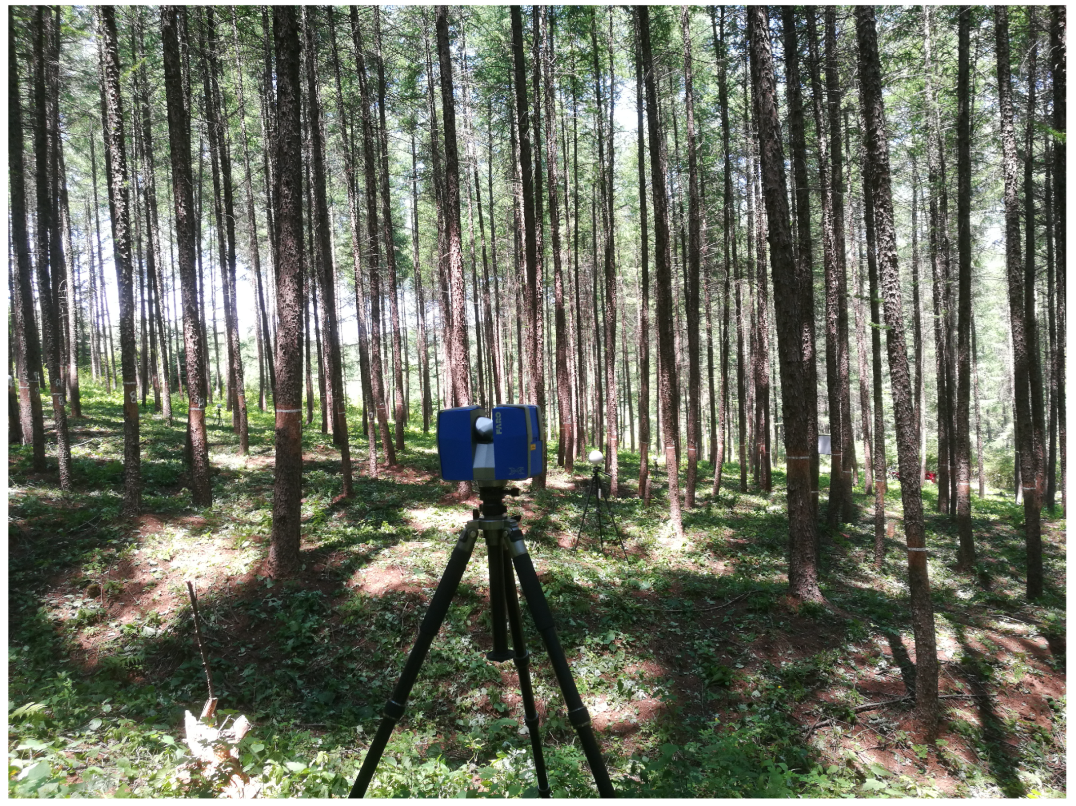
2.1. Field Data Collection

The materials were collected from two field surveys. The two scanning locations were located in the courtyard of the Chinese Academy of Forestry Sciences in Beijing, China, and the Dagujia Forest Farm in Qingyuan County, Liaoning Province, China. The FARO X330 3D terrestrial laser scanner was used for scanning.
Three trees of different species were scanned in the courtyard of the Chinese Academy of Forestry Sciences in Beijing. A Fraxinus pennsylvanica Marsh., a Platanus occidentalis L. and an Ailanthus altissima (Mill.) Swingle were singly scanned from four directions, and two adjacent directions perpendicular to each other, respectively. In the Dagujia Forest Farm, a sample Larix kaempferi plantation plot with a size of 30 m × 30 m was scanned (Figure 1). The scanner worked at the nine stations: the four boundary points of the sample plot, the center points of the four boundary edges, and the center point of the sample plot. A total of 50 trees were scanned in this plot. The scanning parameters of the scanner were the same in the two surveys. The scan quality was 4× (a scanning parameter of the FARO TLS scanner), the scan speed was 122 kpts/s, the point spacing was 6.136 mm at 10 m, and reference spheres were used for point cloud registration in the FARO Scene Software.

2.2. Preprocessing

The tree points and stem points were extracted according to the continuity of the stem in the vertical direction [31]. Affected by unfavorable factors, such as occlusion and breeze, the quality of the scanned tree point cloud has some defects, such as uneven density and incompleteness. The roughness of the stem surface exacerbates the dispersion degree of the stem point cloud. These data deficiencies make it difficult for tree point clouds to effectively reflect the geometric topology and surface roughness of trees, especially at the position above the middle of the stem. In this study, the stem volume was estimated based on a tetrahedral solid model constructed after surface reconstruction. The selected stem point cloud should be able to meet the needs of surface reconstruction; for example, the selected point cloud should be complete. Meanwhile, to accurately compare with traditional volume calculation by sectional measurement, 76 stem segments from 53 trees (some stem segments originate from one stem) with a length of 1 m and below the middle of the stem were chosen for further study.

3. Methodology

The proposed method was divided into three main phases. First, an initial stem segment surface was reconstructed (Figure 2a). Second, the initial stem segment surface was iteratively subdivided by edge subdivision (Figure 2b) and a fine closed disjoint stem segment surface was obtained. Finally, TetGen (Version 1.6.0) software [32] was applied to generate a tetrahedron model of the fine stem segment surface, and the stem segment volume was equal to the sum of the volumes of a series of tetrahedrons in the tetrahedron model.

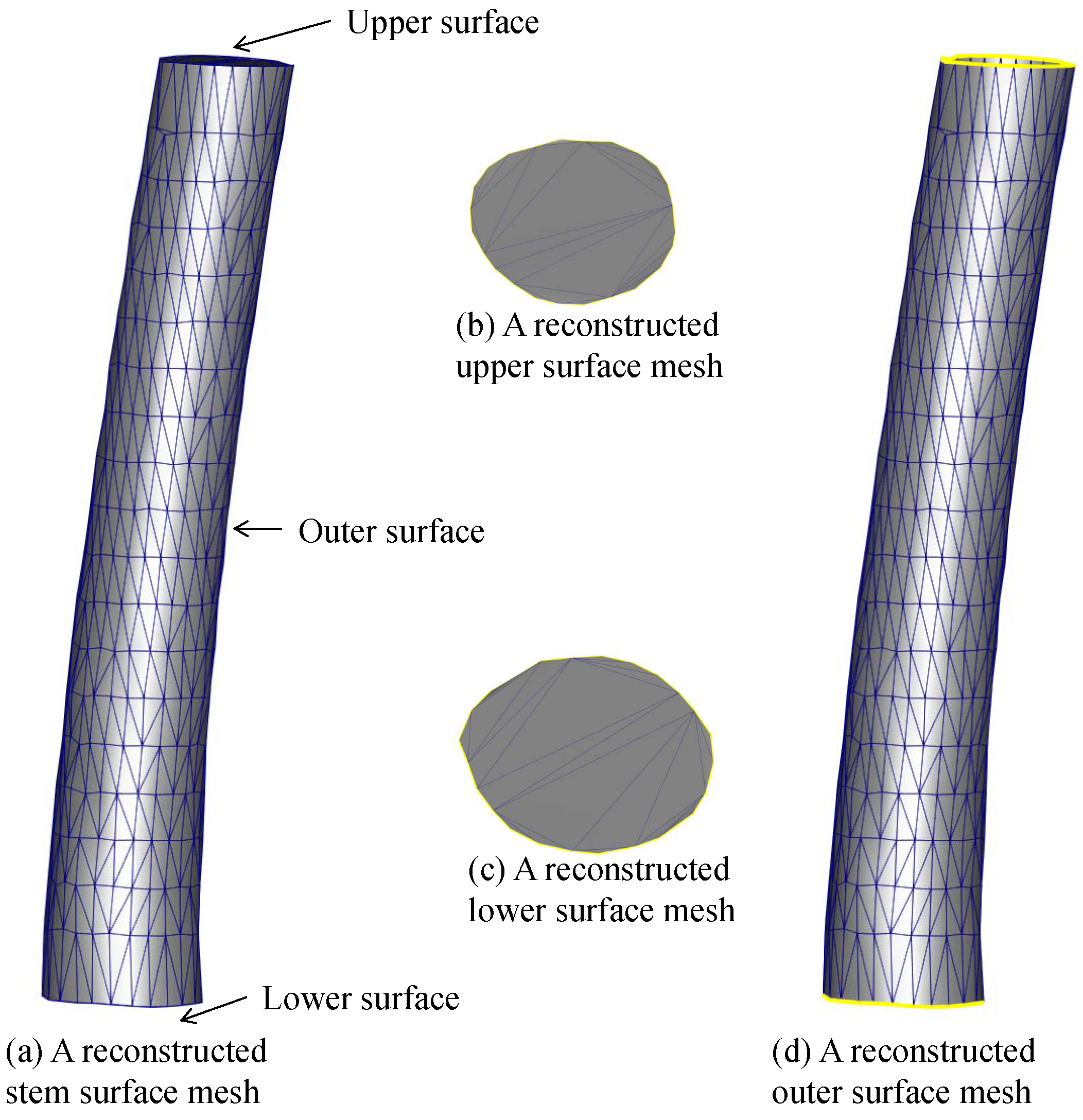
3.1. Initial Stem Segment Surface Reconstruction

3.1.1. Stem Points Downsampling

The stem segment point cloud P was divided horizontally into stem slices at a given height parameter h cm from the bottom to the top of the stem segment. For a stem segment with a length of 100 cm, 100 / h (h is a factor of 100 in this study) stem slices were generated. For a stem slice S i , the geometric central point c p i was calculated by the geometric central point calculation [33]. Then, the angle simplification [33] was adopted, and the stem slice was divided into 360 / ϕ angular regions according to the angle interval parameter ϕ and the angle value η (the included angle between the line segment c p i p k ¯ and the X-axis) between a stem slice point p k and the geometric central point c p i . For an angular region, the average of all the points in the angular region was calculated as the center point of the angular region, and the point in the angular region that was closest to the center point was selected as the sampling point of the angular region. The sampling points of all angular regions constitute a global sampling point set P 0 .

3.1.2. Lower and Upper Surface Reconstruction

Stem segment surface reconstruction includes three parts: lower surface reconstruction, upper surface reconstruction, and outer surface reconstruction (Figure 3).
The lower and upper surface reconstructions can convert constrained Delaunay triangulations of planar point sets. The lower (upper) surface reconstruction is the constrained Delaunay triangulation of a local sampling point set S 0 ( S 100 / h 1 ) from the first (last) stem slice. The constraints are as follows. The planar point set is arranged in counterclockwise order, and a directed edge formed by every two adjacent points in counterclockwise order is the border edge of the constrained Delaunay triangulation. Then, the lower surface mesh M L (Figure 3c) and the upper surface mesh M U (Figure 3b) were obtained by classic constrained Delaunay triangulation.

3.1.3. Outer Surface Reconstruction

The input of outer surface reconstruction includes two parts: the global sampling point set P 0 and border edge set B 0 , which consist of reverse edges of all border edges of the lower surface reconstruction and the upper surface reconstruction. The irregularity of the stem points leads to irregularity of the sampling point set. The method of maximizing the diagonal angle value of the base edge [34,35] was optimized and used to perform the outer surface reconstruction. The optimization strategy is employed to ensure that newly generated triangles do not intersect with existing triangles. The optimized algorithm included two steps: candidate points construction of a base edge and optimal point selection. In the first step, an edge A B was randomly selected from B 0 as the base edge. The candidate point C for the edge A B needs to meet two conditions: (1) the point C is in the point set P 0 S 0 S 100 / h 1 (the point C is in P 0 , but is not in S 0 and S 100 / h 1 ), and (2) the A B C is not directly intersect and not intersect in the projection space with existing triangles formed by points A, B, or C. Points that meet the above two conditions constitute a candidate point set. For the two triangles A B C and D E F , the eigenvector corresponding to the smallest principal component of the vertices of the two triangles was calculated by Principal Component Analysis, then the eigenvector was used as the normal vector of a projection plane, the two projected triangles A B C and D E F by projecting the vertices of the two triangles A B C and D E F onto the projection plane. If the two projected triangles A B C and D E F intersect, the two triangles A B C and D E F intersect in the projection space. In the second step, the point D was selected from candidate points so that the angle value of A D B was the maximum. Then, a new triangle A B D was formed and inserted into outer surface mesh M O , and the edge A B was removed from B 0 . For these two new border edges B D and D A , if they are in B 0 , remove them from B 0 , otherwise, added them to B 0 . Continue to take a border edge (if the edges B D and D A are in B 0 , they should be prioritized as a base edge) from B 0 as a new base edge to perform the above operations until B 0 is empty. If there is no candidate point for a base edge, the height parameter h and the angle interval parameter ϕ should be increased gradually and rolled back to ensure that the optimized algorithm is performed; then, the outer surface mesh M O (Figure 3d) was obtained.
After completing the above operations, an initial stem segment surface mesh M I = M L M U M O (Figure 3a) was reconstructed.

3.2. Stem Segment Surface Subdivision

The initial stem segment surface mesh cannot effectively reflect the geometric characteristics of the unevenness of the stem segment surface. Surface subdivision was performed to refine the initial stem segment surface mesh. There is no need to subdivide the lower surface and the upper surface, as they are planar meshes and have no effect on the stem volume calculation. The surface subdivision was performed on the outer surface mesh M O .
The process of surface subdivision was based on edge subdivision and performed iteratively. The output surface mesh in the ( i 1 ) -th iteration was the input surface mesh M O , i in the i-th iteration. The end condition of the iteration is that there is no edge that can be subdivided. For a directed nonborder directed edge A B in a stem outer surface mesh M O , i in the i-th iteration, its reverse directed edge is B A . The two triangles denoted as A B C and B A D (Figure 4a) can be found by their directed edges A B and B A , respectively. The midpoint of the directed edge A B was denoted as point F. A point denoted as point E in P, which is closest to point F and the distance between them is less than h / 2 , was selected as the subdivision point of the edge subdivision. The two triangles A B C and B A D can be subdivided into four new triangles A E C , E B C , D B E and D E A (Figure 4b), if the four new triangles do not intersect (directly intersect or intersect in the projection space) with any existing triangle formed by points A, B, C, and D, excluding A B C and B A D . If the intersecting relationship is not satisfied, then update the surface mesh M O , i , i.e., the two triangles A B C and B A D are removed from M O , i and four new triangles are added to M O , i ; otherwise, the two directed edges A B and B A cannot be subdivided. Edge subdivision was performed for every pair of directed edges in M O , i , excluding directed edges generated in the i-th iteration.
After the surface subdivision iteration, a more accurate stem segment surface mesh can be obtained (Figure 5). The final triangular surface mesh M of a stem segment can be represented M = M L M U M O , j , where M O , j is the stem segment surface mesh of the last iteration, and different stem segments have different j values.

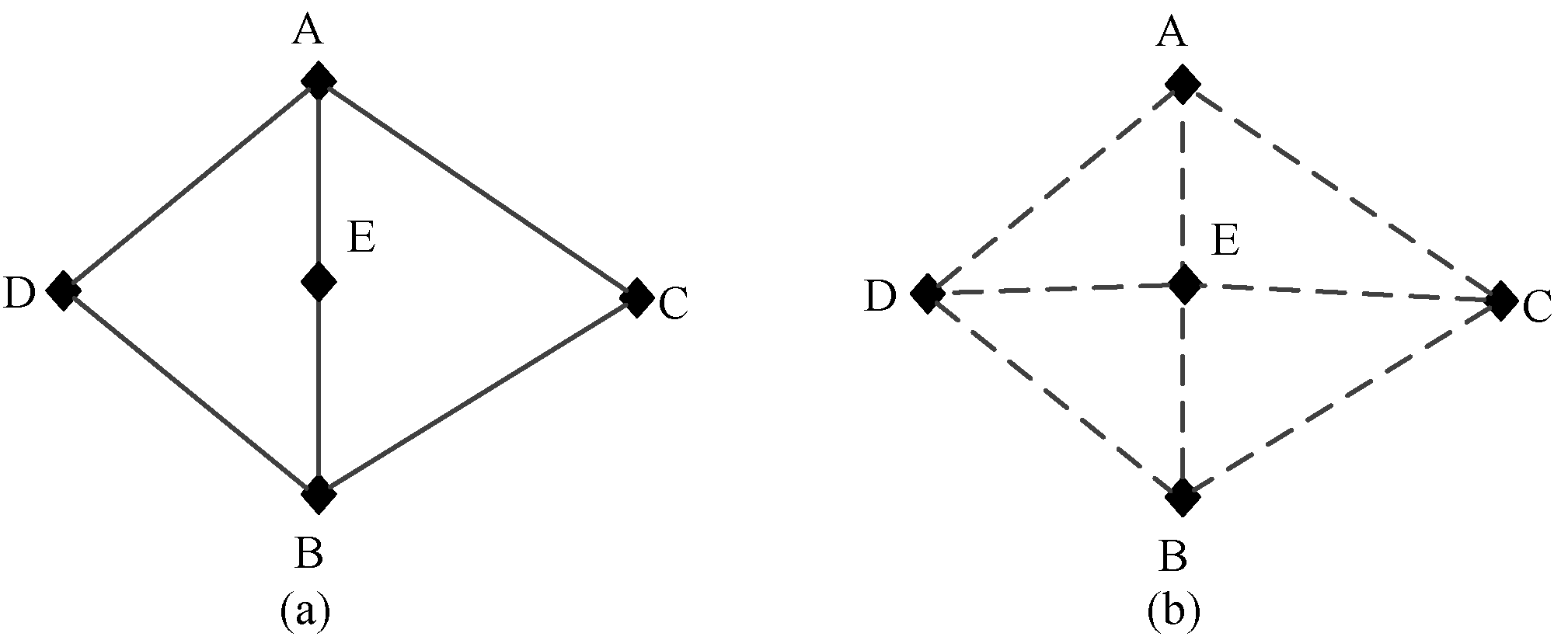
3.3. Tetrahedron Model Generation and Stem Volume Calculation

According to the above step, a final triangular surface mesh M of a stem segment is a closed triangular irregular network, and there is no intersection of triangles. Then, the mesh M of a stem segment can be used as an input of the TetGen [32] software to generate a tetrahedron model of the stem segment. The volume V T of the stem segment is calculated as the sum of the volume of all the tetrahedrons in the tetrahedron model of the stem segment.

3.4. Assessment Method and Indices

The point cloud of the stem segment also provides the essential data for a simulated measurement of the traditional sectional measurement. As described in Section 3.1.1, the stem segment can be divided into 100 / h 0 ( h 0 is a factor of 100, and the value is different from h) stem slices by the given height parameter h 0 cm. Then, the stem diameter D i of the i-th stem slice was retrieved using the existing stem diameter retrieval method from the stem slice point cloud, and the simulated sectional measurement volume V S , i of the i-th stem slice was calculated using Formula (1). The stem volume V S of the stem segment was calculated using Formula (2), and used as a reference value in this study.
V S , i = π × h 0 × D i 2 / 4
V S = i = 1 100 / h 0 V S , i
It is obvious that the smaller the h 0 value is, the larger the number of stem slices, and the more accurate the volume. Therefore, h 0 in this study was set to 1 cm, which is exactly the width of the diameter tape. Compared with the field-measured stem diameter at breast height, the RMSEs of the cylinder fitting and circle fitting were all 0.30 cm, and the two methods were the best and most robust of the six stem diameter retrieval methods [16]. Circle fitting works in 2D spaces and is more convenient than cylinder fitting; therefore, the circle fitting method was selected for stem diameter retrieval in this study.
According to the simulated sectional measurement, 100 pieces of stem diameters can be measured along a stem segment. The average stem diameter D g and the stem diameter difference D e between the minimum and maximum stem diameters were calculated for a stem segment.
Based on V T , the average stem diameter D v of the stem segment estimated from V T can be represented as Formula (3).
D v = 2 × V T / π / 100
The accuracy of the stem segment volume was evaluated using root mean square error (RMSE), relative root mean square error (RRMSE), R-squared (R2), mean absolute error (MAE), and mean absolute percentage error (MAPE).
The Hausdorff distance (HD) between the original stem segment point cloud and the reconstructed stem segment surface was used to evaluate the accuracy of the reconstructed stem segment surface.
Our method was implemented using C++ with the Point Cloud Library [36], Qt, and VTK.

4. Results

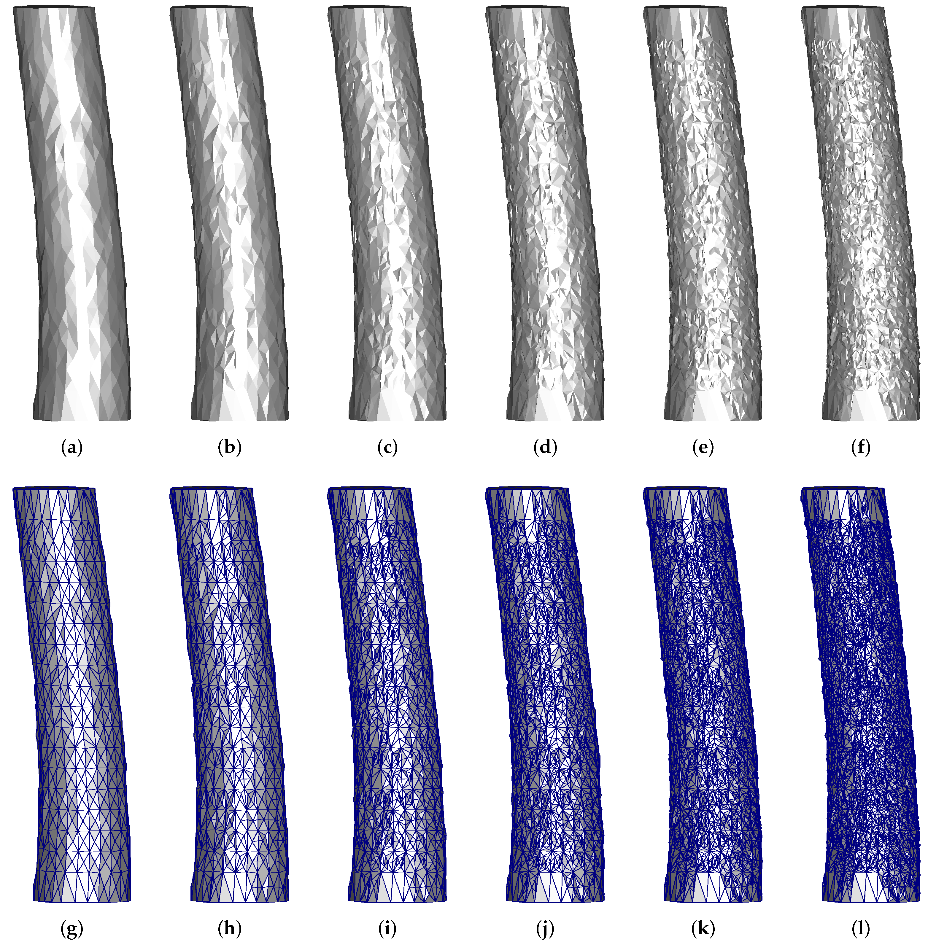
4.1. Volume Calculation of a Stem Segment under Different Iterations

The initial stem segment surface mesh can be subdivided to obtain a more detailed surface mesh. The visual effects of surfaces and surface meshes of a stem segment (the average stem diameter of this stem segment was 14.40 cm) from the Larix kaempferi tree under different iterations are shown in Figure 5.
The initial reconstructed surface is smooth in some local zones (Figure 5a); correspondingly, the triangle in the initial reconstructed surface mesh is very large (Figure 5g). As the number of iterations increases, the roughness of the stem surface is gradually reflected (Figure 5b–f), and most of the triangles become increasingly smaller (Figure 5h,i). According to Figure 5f, the unevenness of the stem surface is the most obvious, and the number of triangles in Figure 5i is the largest. The results showed that the surface model of the stem segment becomes closer to the true surface of the stem segment during the iterative subdivision. This means that the stem segment volume calculated based on the next subdivision surface model will be closer to the true value of the stem volume than the stem segment volume calculated by the current subdivision surface model.
From Table 1, the HD, the number of triangles, and the number of tetrahedrons increase with the number of iterations. The increased number of triangles and tetrahedrons demonstrated that the surface model, and the solid model of the stem segment in the current iteration were more delicate than those in the previous iteration. The more delicate the surface model and the solid model are, the more accurate the volume of the stem segment. This is also reflected in the values of V T in Table 1, which increased with the number of iterations and approached V S . The increased HD demonstrated that the distance between the minority points and the reconstructed stem surface increased with the number of iterations.

4.2. Volume Calculation of a Stem Segment Using Different Parameters

As described in Section 3.1.3, the height parameter h and the angle interval parameter ϕ can be adjusted to obtain the outer surface mesh M O . It means that for a stem segment, multiple outer surface meshes M O can be reconstructed using different parameters, resulting in different final triangular surface meshes M at different iteration numbers, and multiple different volumes with different accuracies. The reconstructed stem surface models using different parameters for the stem segment in Figure 5 are shown in Figure 6.
Figure 6 shows that the density of the triangles in the stem surface model in Figure 6g,h is higher than that in Figure 6i–l. Correspondingly, the fineness level of the stem surface in Figure 6a,b is higher than that in Figure 6c–f. This demonstrated by the fact that when using a small height parameter h, it is more effective to reflect the surface characteristics of the stem. According to the effect of graphics, it is reasonable to assume that the more triangles there are in the surface model, the more accurate the surface model, and the more tetrahedrons there are, the more accurate the calculated volume will be.
According to Table 2, when the height parameter h increases, the number of iterations and HD tend to increase, and the number of triangles, the number of tetrahedrons, and the stem segment volume V T tend to decrease. All the stem segment volumes V T by the tetrahedron model are smaller than the stem segment volumes V S calculated using simulated sectional measurements. The minimized and maximized volume errors between different V T with different parameters were 7.08 (0.04%, as a percentage of V S , the same as below) and 98.54 cm3 (0.60%). Considering that the length of the stem segment was 100 cm, the average stem diameter was 14.40 cm and the minimum and maximum volume errors between V T and V S were 119.93 (0.73%) and 200.53 cm3 (1.22%),respectively, the volume error between different V T with different parameters may be acceptable.
According to Figure 6, the stem surface patches near the top and the bottom of the stem segment were not subdivided very thoroughly, which accelerated with parameters h and ϕ . It is obvious that the more surface subdivisions there are, the more accurate the surface model and the tetrahedron model, and the more accurate the stem segment volume. Meanwhile, the areas of triangles in these stem surface patches using smaller parameters were smaller than those using larger parameters. It also demonstrated that the smaller parameters can result in a more accurate stem segment volume if the surface model can be successfully constructed using these smaller parameters.

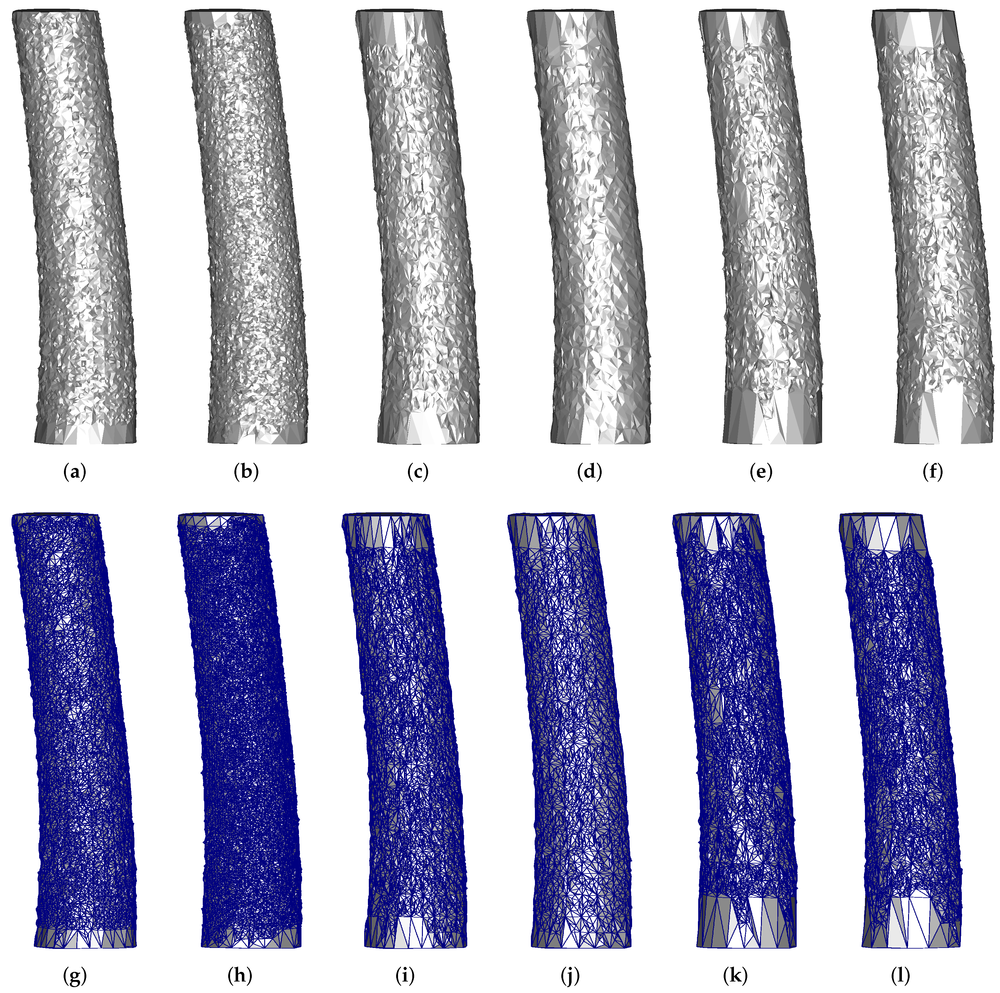
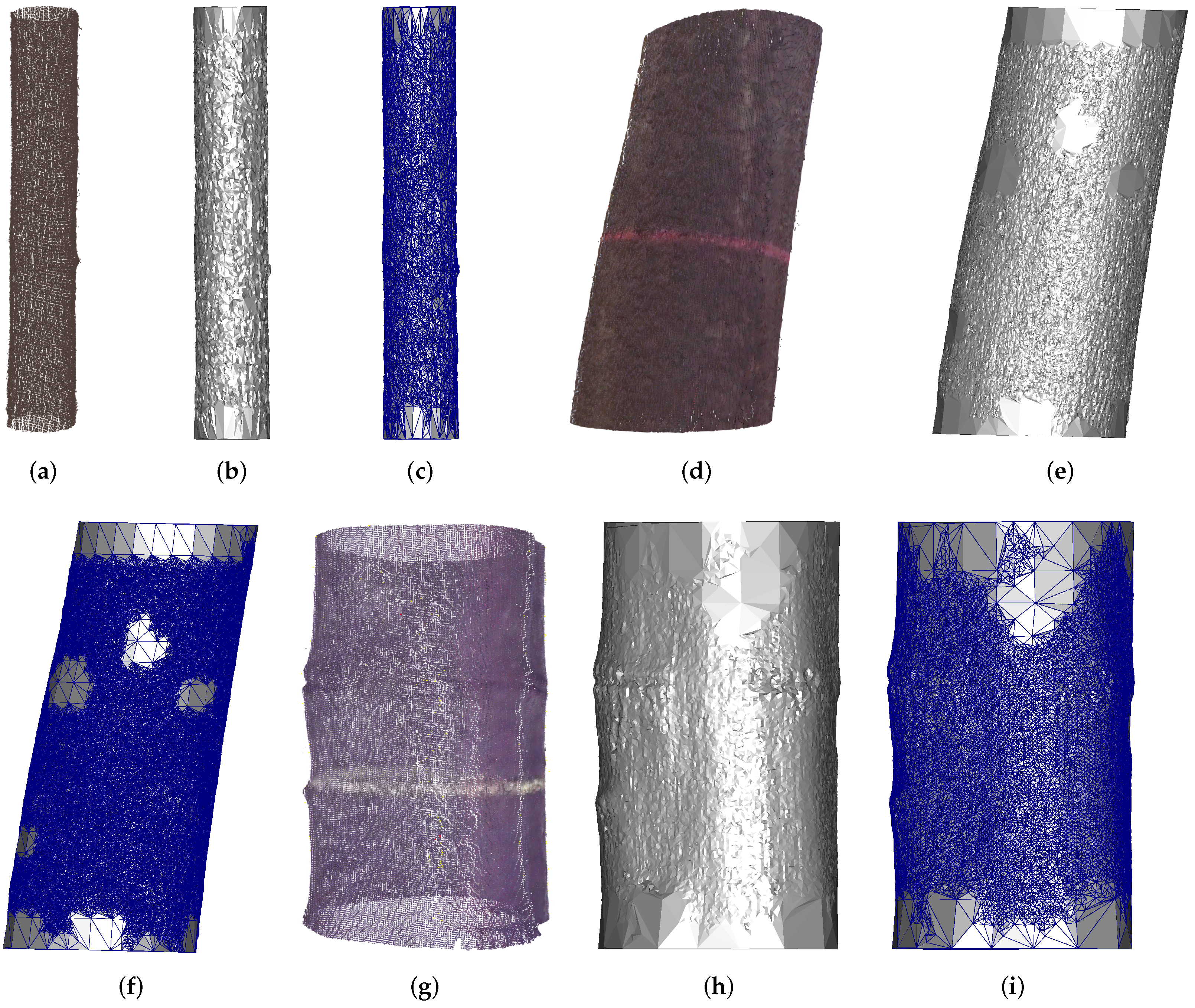
4.3. Surface Models of Stem Segments from Different Tree Species

Trees of different species have different surface geometry features, and reconstructed surface models from different tree species should reflect this difference. The final reconstructed triangular surfaces and surface meshes of three stem segments from three tree species are shown in Figure 7. The bark in Figure 7a is the roughest, followed by that in Figure 7d, and the bark in Figure 7g is the smoothest. Although the subdivision of the surface model is not completely uniform, the reconstructed stem surfaces can faithfully reflect the above bark geometry feature. Notably, the convex and concave features of the tree surface are fully represented in the reconstructed stem surface (Figure 7g–i). This means that regardless of the tree species, the reconstructed surface model can approximate to the true surface of the stem segment, and the corresponding tetrahedron model can also be close to the solid structure of the stem segment; correspondingly, the calculated volume based on the tetrahedron model can approach its true value.

4.4. Tetrahedron Models of Stem Segments

The slices of the tetrahedron models on the x-axis are shown in Figure 8. The angle of view was adjusted to highlight the slices of the tetrahedron models. The composition of the internal tetrahedrons is clearly shown in Figure 8. The surface models in Figure 5l and Figure 6l are different for the same stem segment; therefore, Figure 8a,b shows different tetrahedron models for the same stem segment. As the stem segment volume is equal to the sum of the volumes of all the tetrahedrons, and the internal tetrahedrons are adjacent to each other, the size of the internal tetrahedrons will not affect the calculation of the stem segment volume, if the stem segment surface model is close enough to the actual surface of the stem segment. This demonstrated the importance of the stem surface reconstruction method in the presented method.

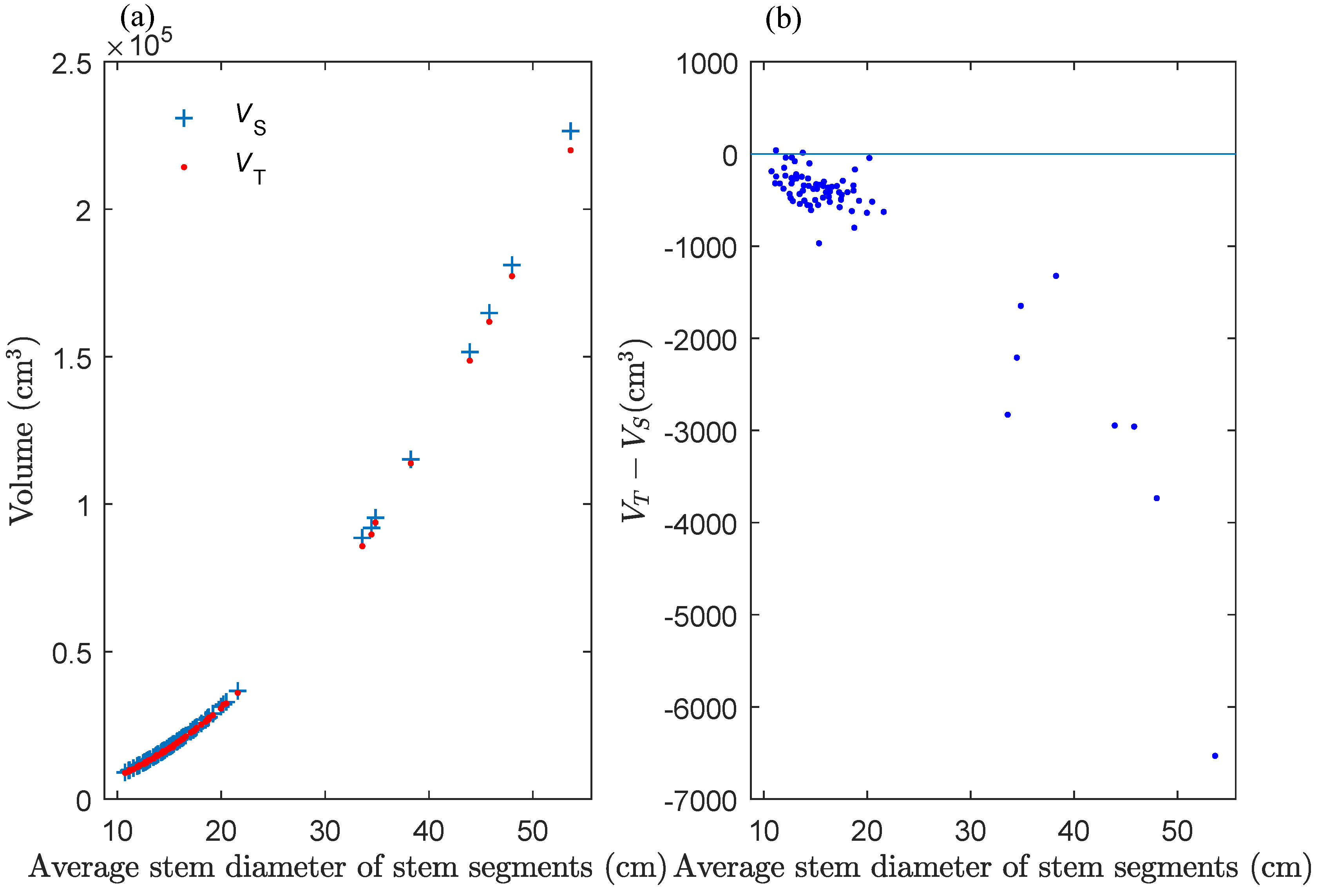
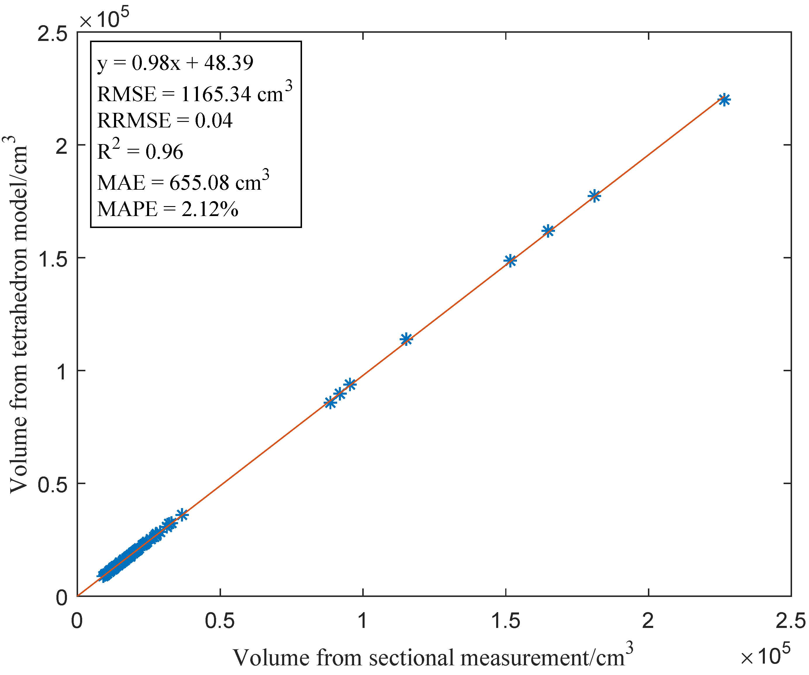
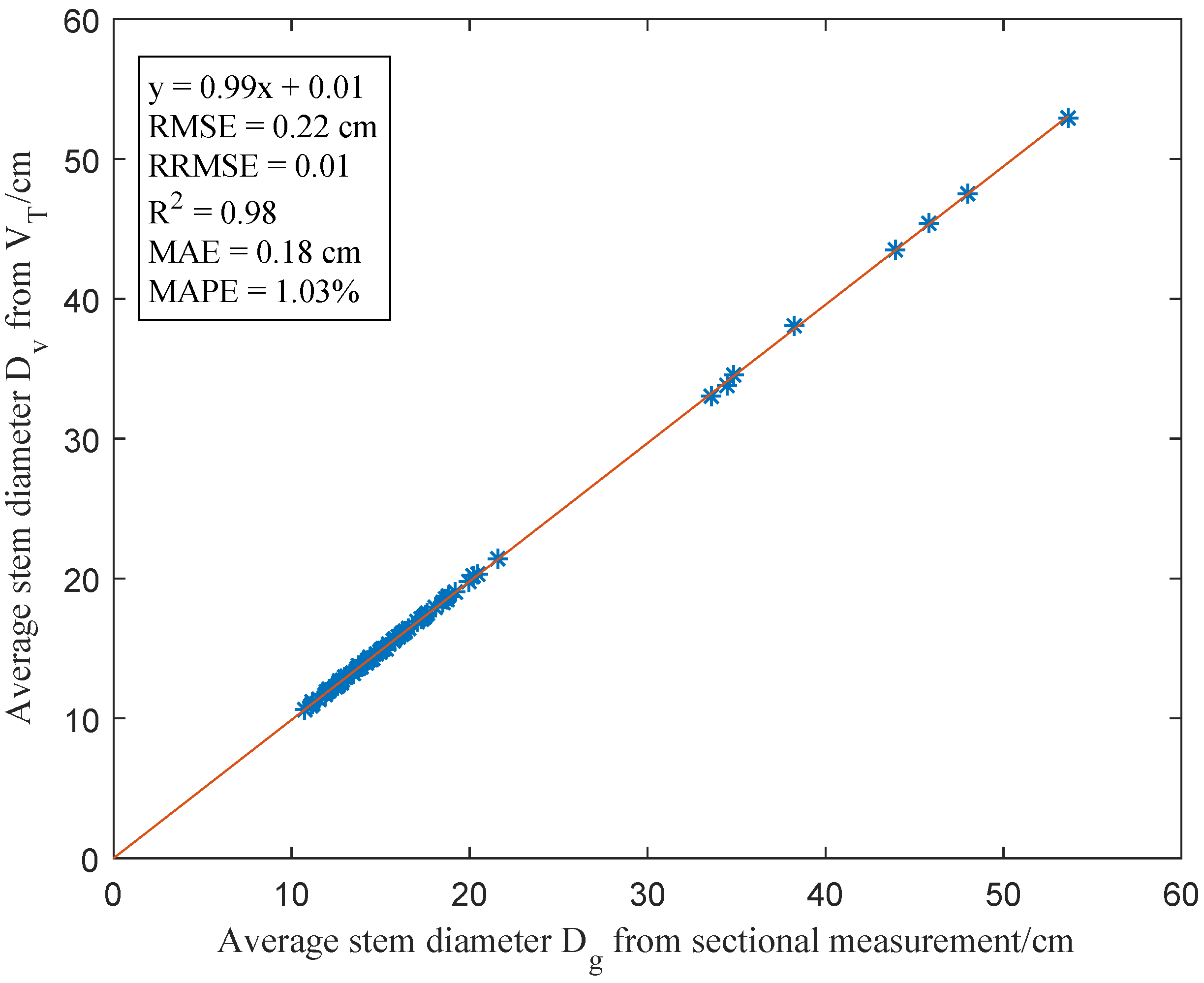
4.5. Numerical Results

The minimum, maximum, and average stem diameter differences and V S for all the studied stem segments were obtained (Table 3). According to the tetrahedron model for stem segment volume calculation, the minimum, maximum, and average of HD, the number of triangles and tetrahedrons, V T , and the volume difference V e between V S and V T , were calculated (Table 3).
The data of D g show that most stem diameters of the studied stem segments were not large. The average of D e means that the difference in stem diameters of a stem diameter was not great. The HD data show that the HD between the stem segment point cloud and the reconstructed stem segment surface was not small. The data of the number of triangles and the number of tetrahedrons means that there were many triangles, and tetrahedrons belong to the reconstructed stem segment surface model and the stem segment tetrahedron model. The data of V e show that most V S were larger than V T . There were only two exceptions (as shown in Figure 9b).
The relationship between V T , V S , and these average stem diameters is shown in Figure 9. Although stem diameters larger than 25 cm are rare, the relationship between the average stem diameters and volumes formed by the data points is clear. The difference between V T and V S increased with the average stem diameter.
The regression equation and assessment index values between V T and V S are shown in Figure 10. The values of the assessment indexes demonstrated that there is a certain degree of deviation between V T and V S .
The regression equation and assessment index values between D g and D v are shown in Figure 11. Although the difference between D g and D v was not so obvious, there must be a difference between D g and D v . This also reflects the volume difference between the two measurement methods from one side.

5. Discussion

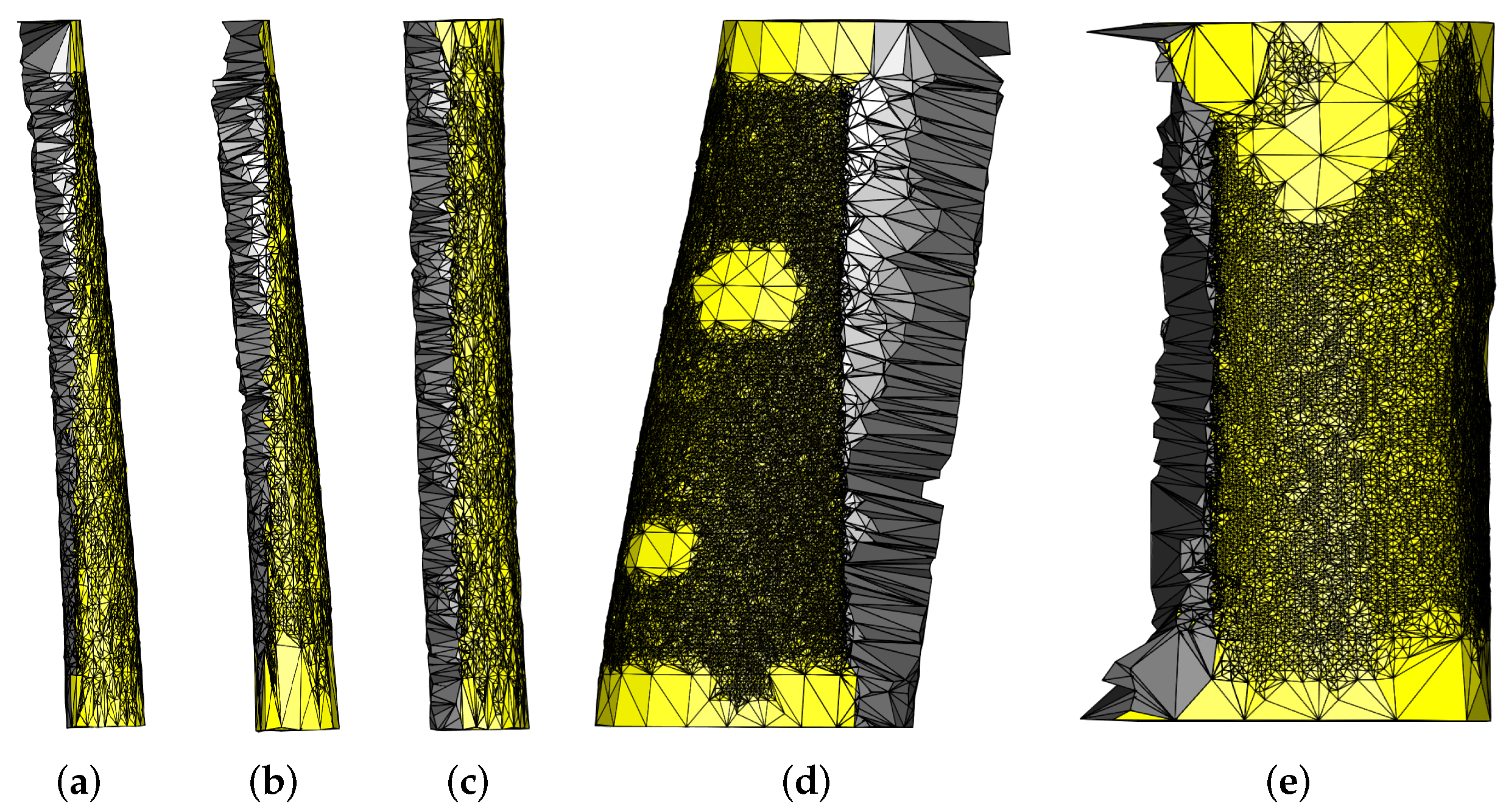
5.1. The Complexity of Stem Surface Reconstruction

Surface reconstruction is a common technology in computer-aided design and computer graphics. The basic assumption of surface reconstruction in these fields is that the underlying surface of the reconstructed object is smooth [37], i.e., the point cloud scanned from the reconstructed object is manifold, and the basic requirement of solid model reconstruction is that the surface model of the reconstructed object is closed and disjoint [32]. However, the scanned point cloud from the tree is not manifold due to the irregularity of the stem or the roughness of the stem bark. This determines the complexity of the tree surface reconstruction. Ref. [27] tried to reconstruct the stem surface using TLS data, and the visual quality of reconstructed meshes by the Poisson surface reconstruction method provided by the software MeshLab (Version 1.3.2) showed that the reconstructed stem model cannot describe the actual stem, especially for irregular trees. In this study, the step of stem point downsampling in Section 3.1.1 is essentially sampling to make the input point cloud for the initial stem segment surface reconstruction manifold, thereby ensuring that the stem surface can be initially constructed. The surface subdivision ensures that the reconstructed stem surface is as close as possible to the actual stem surface (Figure 5, Figure 6 and Figure 7), although there were some zones where the surface model cannot be subdivided.
The parameters h and ϕ can be adjusted to reconstruct an initial surface model of a stem segment in this study. Although different parameters result in different surface models, different tetrahedron models, and different volumes, fortunately, the volume difference obtained in the reconstructed tetrahedral solid model after surface subdivision was not very large (Table 2). It demonstrates the feasibility of surface reconstruction of stem segments with different stem surface roughness and different point cloud densities, i.e., if the initial surface model cannot be obtained using smaller parameters h and ϕ , the two parameters h and ϕ can be increased separately to perform the outer surface reconstruction. Sometimes, the parameters h and ϕ must be increased to obtain a closed disjoint surface model.

5.2. The Accuracy of the Stem Segment Volume Using the Tetrahedron Model

The simulated sectional measurement was used as the reference method in this study. The thickness of the stem slice point cloud in the simulated sectional measurement was 1 cm. Measuring stem diameter at every 1 cm is very difficult to implement in the field inventory, even for stem analysis. The stem diameter of the stem slice point cloud was retrieved by the circle fitting method, the accuracy of which has been verified in many studies [10,16,38]. Therefore, the accuracy of the simulated sectional measurement in this study has the reference value.
The traditional sectional measurement is based on the assumption that the stem cross-section is a circle. However, the actual stem cross-section is not a regular geometry. This brings imprecise factors into the calculation of the basal area and volume of the stem. The area of a circle is the largest when the circumference is fixed. Therefore, the volume of a stem slice by the simulated sectional measurement is the largest volume in theory. Considering the actual geometric structure of the stem segment, there must be an error between the true volume value and the volume using the simulated sectional measurement. This is exactly the reason that most V T were lower than V S . Notably, the shape of a stem cross-section is related to the diameter of the stem cross-section. The lower the stem diameter, the closer the shape of the stem cross-section is to a circle, and the lower the deformation along the stem segment. This can be explained by the fact that the lower the average stem diameter was, the lower the difference between V T and V S was.
In this study, stem segment volumes were calculated based on tetrahedron models constructed after surface reconstruction. The initial stem segment surface reconstruction and the surface subdivision were all performed based on the original point cloud of the stem segment. Therefore, the surface model and the tetrahedron model were the closest geometric models to the actual surface and the solid structure of the stem segment in theory, respectively. This is truly the value of surface reconstruction and solid reconstruction. Therefore, the stem segment volume calculated based on the tetrahedron model is the most accurate in theory. For a stem segment, there are many initial stem segment surface models that can be reconstructed using different parameters h and ϕ in this study. Different parameters mean different surface models, different tetrahedron models, and different stem segment volumes (Table 2). Fortunately, the differences between these volumes are acceptable. Therefore, the stem segment volume using the tetrahedron model is closer to the true volume value than that using sectional measurement.
The volume calculation of the empirical volume formula is based on retrieval stem parameters and pre-established empirical formulas. This method depends not only on traditional measurement methods, but also on stem parameter retrieval methods using TLS data. The volume calculation based on the QSM and regular geometry model assumed that the stem cross-section is a circle. The irregularity of the stem cross-section is overlooked. The existing irregularity geometry model method in [27] considered the irregularity of the stem cross-section. The voxel-based bounding box method [28] relies on the voxel size and cannot output a watertight geometrical model. In this study, the stem segment was reconstructed using the surface model and tetrahedron model. The irregularities along the stem segment and belonging to the stem cross-section were all considered. The constructed surface model and tetrahedron model were all watertight geometrical models that can represent the geometrical features of the stem segment. Meanwhile, the volume can be directly calculated by a series of tetrahedrons in the tetrahedron model. Although the stem volume for a whole stem was not estimated in this study, considering that the stem volume is traditionally calculated in sections, the volume of a whole stem can be estimated by section reconstruction if the point cloud is satisfactory. Therefore, the volume calculation using the tetrahedron model is superior to the existing stem volume calculations using TLS data.

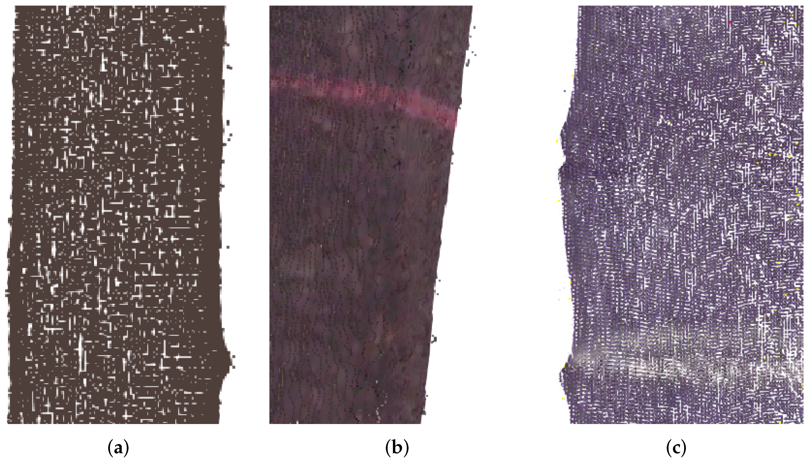
5.3. The Importance of the Quality of the Stem Point Cloud

The point cloud quality at different stem heights is different as the distance between the stem and the TLS scanner changes with the height. It is difficult to use the same parameters to reconstruct a surface model for a whole stem. This is also the reason for calculating the volume in the stem segment in this study. Stem volume calculation by stem segments is also a conventional method in forest inventory using traditional measuring tools. Therefore, the accuracy of the stem segment volume calculation can be regarded as the accuracy of the stem volume calculation.
The stem bark is rough, convex, and concave, and the texture of the stem bark changes from extremely rough to quite smooth [5]. The different stem geometrical features are shown in Figure 7. Even if the bark is very smooth, there is still some debris such as fallen bark attached to the bark. The debris may introduce noise into the stem point cloud. The point cloud scanned by multiple stations will also generate noise during point registration. Once these noises approach the points that are reflected from the actual stem surface, they are difficult to detect. The irregularity of the stem surface, the roughness of the stem bark, the disturbance of noises, and the combination of these factors leads to the complexity of the stem point cloud. Points in the stem point cloud cannot all be vertices of triangles in the stem surface model, which is the reason for the HD in this study. The existence of noise further increased the value of HD (as the scattered points along stem surfaces shown in Figure 12, it can also be seen in the enlarged view of Figure 7). Therefore, preprocessing the input stem point cloud and improving the quality of the point cloud will not only help to build a higher quality surface model, but also reduce the HD value, and, more importantly, output a more accurate stem segment volume.
This study focuses on a numerical method for stem volume estimation, which downsamples the input point cloud and adjusts parameters to meet the volume estimation of stem segments with different point cloud densities. The impact of point cloud quality on volume estimation accuracy has not been thoroughly studied. Improving the quality of stem point clouds as part of data collection and preprocessing is still a future concern.

6. Conclusions

In this study, we proposed a stem segment volume estimation based on the tetrahedron model that depends on the surface model. The visualization results showed that the reconstructed surface model can reflected the convex and concave features of the stem segment. This means that the constructed tetrahedron model of the stem segment can approximate the solid space occupied by the stem segment. The numerical results showed that most stem segment volumes estimated by the tetrahedron model V T were lower than those estimated by simulated sectional measurements V S . The average difference between V T and V S was 655.12 cm3. Compared with V S , the RMSE of V T was 1165.34 cm3.
The irregularity of the stem makes it difficult to directly estimate its volume using conventional measuring tools. Most existing stem volume estimations assume that the geometry of the stem cross-section is regular. Unlike existing methods, we considered the irregularity of the stem, and calculated the stem segment volume directly from the constructed tetrahedron model of the stem segment using surface and solid reconstruction methods. This provides an efficient way to reflect the complex geometrical features of the stem surface and to retrieve stem volume accurately while considering the irregularity of the stem.

Author Contributions

Conceptualization, software and writing—original draft preparation, L.Y.; data processing, software, validation and investigation, X.C.; investigation and data processing, Y.S.; investigation, writing—review and editing, Y.P.; investigation, writing—review and editing, Y.F.; writing—review and editing, X.S. All authors have read and agreed to the published version of the manuscript.

Funding

This research was supported by the National Natural Science Foundation of China (No.31872704), the Foundation for Distinguished Young Talents in Higher Education of Henan (No.2020GGJS157), the Xinyang Academy of Ecological Research Open Foundation (No.2023XYMS12) and the Nanhu Scholars Program for Young Scholars of XYNU.

Data Availability Statement

The data presented in this study are available on request from the corresponding author.

Conflicts of Interest

The authors declare no conflict of interest.

References

  1. Abegg, M.; Bösch, R.; Kükenbrink, D.; Morsdorf, F. Tree volume estimation with terrestrial laser scanning—Testing for bias in a 3D virtual environment. Agric. For. Meteorol. 2023, 331, 109348. [Google Scholar] [CrossRef]
  2. Yusup, A.; Halik, Ü.; Keyimu, M.; Aishan, T.; Abliz, A.; Dilixiati, B.; Wei, J. Trunk volume estimation of irregular shaped Populus euphratica riparian forest using TLS point cloud data and multivariate prediction models. For. Ecosyst. 2023, 10, 100082. [Google Scholar] [CrossRef]
  3. An, Z.; Froese, R.E. Tree stem volume estimation from terrestrial LiDAR point cloud by unwrapping. Can. J. For. Res. 2023, 53, 60–70. [Google Scholar] [CrossRef]
  4. Demol, M.; Verbeeck, H.; Gielen, B.; Armston, J.; Burt, A.; Disney, M.; Duncanson, L.; Hackenberg, J.; Kükenbrink, D.; Lau, A.; et al. Estimating forest above-ground biomass with terrestrial laser scanning: Current status and future directions. Methods Ecol. Evol. 2022, 13, 1628–1639. [Google Scholar] [CrossRef]
  5. West, P.W. Tree and Forest Measurement; Springer: Berlin/Heidelberg, Germany, 2009. [Google Scholar]
  6. Xianyu, M. Forest Measuration; China Forestry Publishing House: BeiJing, China, 2006. [Google Scholar]
  7. Van Laar, A.; Akca, A. Forest Mensuration; Springer Science & Business Media: Berlin/Heidelberg, Germany, 2007; Volume 13. [Google Scholar]
  8. Leäo, F.M.; Nascimento, R.G.M.; Emmert, F.; Santos, G.G.A.; Caldeira, N.A.M.; Miranda, I.S. How many trees are necessary to fit an accurate volume model for the Amazon forest? A site-dependent analysis. For. Ecol. Manag. 2021, 480, 118652. [Google Scholar] [CrossRef]
  9. Liang, X.; Kankare, V.; Hyyppä, J.; Wang, Y.; Kukko, A.; Haggrën, H.; Yu, X.; Kaartinen, H.; Jaakkola, A.; Guan, F.; et al. Terrestrial laser scanning in forest inventories. ISPRS J. Photogramm. Remote Sens. 2016, 115, 63–77. [Google Scholar] [CrossRef]
  10. Liang, X.; Hyyppä, J.; Kaartinen, H.; Lehtomäki, M.; Pyörälä, J.; Pfeifer, N.; Holopainen, M.; Brolly, G.; Francesco, P.; Hackenberg, J.; et al. International benchmarking of terrestrial laser scanning approaches for forest inventories. ISPRS J. Photogramm. Remote Sens. 2018, 144, 137–179. [Google Scholar] [CrossRef]
  11. Calders, K.; Adams, J.; Armston, J.; Bartholomeus, H.; Bauwens, S.; Bentley, L.P.; Chave, J.; Danson, F.M.; Demol, M.; Disney, M.; et al. Terrestrial laser scanning in forest ecology: Expanding the horizon. Remote Sens. Environ. 2020, 251, 112102. [Google Scholar] [CrossRef]
  12. Cabo, C.; Ordóñez, C.; López-Sánchez, C.A.; Armesto, J. Automatic dendrometry: Tree detection, tree height and diameter estimation using terrestrial laser scanning. Int. J. Appl. Earth Obs. Geoinf. 2018, 69, 164–174. [Google Scholar] [CrossRef]
  13. Michałowska, M.; Rapiński, J.; Janicka, J. Tree position estimation from TLS data using hough transform and robust least-squares circle fitting. Remote Sens. Appl. Soc. Environ. 2023, 29, 100863. [Google Scholar] [CrossRef]
  14. Pitkänen, T.P.; Raumonen, P.; Kangas, A. Measuring stem diameters with TLS in boreal forests by complementary fitting procedure. ISPRS J. Photogramm. Remote Sens. 2019, 147, 294–306. [Google Scholar] [CrossRef]
  15. Ravaglia, J.; Fournier, R.A.; Bac, A.; Véga, C.; Côté, J.F.; Piboule, A.; Rémillard, U. Comparison of Three Algorithms to Estimate Tree Stem Diameter from Terrestrial Laser Scanner Data. Forests 2019, 10, 599. [Google Scholar] [CrossRef]
  16. You, L.; Wei, J.; Liang, X.; Lou, M.; Pang, Y.; Song, X. Comparison of Numerical Calculation Methods for Stem Diameter Retrieval Using Terrestrial Laser Data. Remote Sens. 2021, 13, 1780. [Google Scholar] [CrossRef]
  17. Srinivasan, S.; Popescu, S.C.; Eriksson, M.; Sheridan, R.D.; Ku, N.W. Terrestrial Laser Scanning as an Effective Tool to Retrieve Tree Level Height, Crown Width, and Stem Diameter. Remote Sens. 2015, 7, 1877–1896. [Google Scholar] [CrossRef]
  18. Sun, J.; Wang, P.; Li, R.; Zhou, M.; Wu, Y. Fast Tree Skeleton Extraction Using Voxel Thinning Based on Tree Point Cloud. Remote Sens. 2022, 14, 2558. [Google Scholar] [CrossRef]
  19. Xu, Y.; Hu, C.; Xie, Y. An improved space colonization algorithm with DBSCAN clustering for a single tree skeleton extraction. Int. J. Remote Sens. 2022, 43, 3692–3713. [Google Scholar] [CrossRef]
  20. Panagiotidis, D.; Abdollahnejad, A. Accuracy Assessment of Total Stem Volume Using Close-Range Sensing: Advances in Precision Forestry. Forests 2021, 12, 717. [Google Scholar] [CrossRef]
  21. Ninni Saarinen, V.K.; Vastaranta, M.; Luoma, V.; Pyörälä, J.; Tanhuanpää, T.; Liang, X.; Kaartinen, H.; Kukko, A.; Jaakkola, A.; Yu, X.; et al. Feasibility of Terrestrial laser scanning for collecting stem volume information from single trees. ISPRS J. Photogramm. Remote Sens. 2017, 123, 140–158. [Google Scholar] [CrossRef]
  22. Calders, K.; Newnham, G.; Burt, A.; Murphy, S.; Raumonen, P.; Herold, M.; Culvenor, D.; Avitabile, V.; Disney, M.; Armston, J.; et al. Nondestructive estimates of above-ground biomass using terrestrial laser scanning. Methods Ecol. Evol. 2015, 6, 198–208. [Google Scholar] [CrossRef]
  23. Brede, B.; Calders, K.; Lau, A.; Raumonen, P.; Bartholomeus, H.M.; Herold, M.; Kooistra, L. Non-destructive tree volume estimation through quantitative structure modelling: Comparing UAV laser scanning with terrestrial LIDAR. Remote Sens. Environ. 2019, 233, 111355. [Google Scholar] [CrossRef]
  24. Brede, B.; Terryn, L.; Barbier, N.; Bartholomeus, H.M.; Bartolo, R.; Calders, K.; Derroire, G.; Krishna Moorthy, S.M.; Lau, A.; Levick, S.R.; et al. Non-destructive estimation of individual tree biomass: Allometric models, terrestrial and UAV laser scanning. Remote Sens. Environ. 2022, 280, 113180. [Google Scholar] [CrossRef]
  25. Raumonen, P.; Kaasalainen, M.; Åkerblom, M.; Kaasalainen, S.; Kaartinen, H.; Vastaranta, M.; Holopainen, M.; Disney, M.; Lewis, P. Fast Automatic Precision Tree Models from Terrestrial Laser Scanner Data. Remote Sens. 2013, 5, 491. [Google Scholar] [CrossRef]
  26. Fan, G.; Nan, L.; Dong, Y.; Su, X.; Chen, F. AdQSM: A New Method for Estimating Above-Ground Biomass from TLS Point Clouds. Remote Sens. 2020, 12, 3089. [Google Scholar] [CrossRef]
  27. Nölke, N.; Fehrmann, L.; I Nengah, S.; Tiryana, T.; Seidel, D.; Kleinn, C. On the geometry and allometry of big-buttressed trees-a challenge for forest monitoring: New insights from 3D-modeling with terrestrial laser scanning. IForest-Biogeosci. For. 2015, 8, 574. [Google Scholar] [CrossRef]
  28. Hess, C.; Bienert, A.; Härdtle, W.; Von Oheimb, G. Does Tree Architectural Complexity Influence the Accuracy of Wood Volume Estimates of Single Young Trees by Terrestrial Laser Scanning? Forests 2015, 6, 3847–3867. [Google Scholar] [CrossRef]
  29. Bienert, A.; Hess, C.; Maas, H.G.; Von Oheimb, G. A voxel-based technique to estimate the volume of trees from terrestrial laser scanner data. Int. Arch. Photogramm. Remote Sens. Spat. Inf. Sci. 2014, 40, 101–106. [Google Scholar] [CrossRef]
  30. Pitkänen, T.P.; Raumonen, P.; Liang, X.; Lehtomäki, M.; Kangas, A. Improving TLS-based stem volume estimates by field measurements. Comput. Electron. Agric. 2021, 180, 105882. [Google Scholar] [CrossRef]
  31. Liu, L.; Pan, g.Y.; Li, Z. Individual Tree DBH and Height Estimation Using Terrestrial Laser Scanning (TLS) in A Subtropical Forest. Sci. Silvae Sin. 2016, 52, 26–37. [Google Scholar] [CrossRef]
  32. Si, H. TetGen, a Delaunay-Based Quality Tetrahedral Mesh Generator. ACM Trans. Math. Softw. 2015, 41, 11. [Google Scholar] [CrossRef]
  33. You, L.; Tang, S.; Song, X.; Lei, Y.; Zang, H.; Lou, M.; Zhuang, C. Precise Measurement of Stem Diameter by Simulating the Path of Diameter Tape from Terrestrial Laser Scanning Data. Remote Sens. 2016, 8, 717. [Google Scholar] [CrossRef]
  34. Maus, A. Delaunay Triangulation and the Convex Hull Of n Points in Expected Linear Time. BIT 1984, 24, 151–163. [Google Scholar] [CrossRef]
  35. You, L.; Tang, S.; Song, X. Growth algorithm centered on priority point for constructing the Delaunay triangulation. J. Image Graph. 2016, 21, 60–68. [Google Scholar]
  36. Rusu, R.B.; Cousins, S. 3D is here: Point cloud library (pcl). In Proceedings of the 2011 IEEE International Conference on Robotics and Automation, Shanghai, China, 9–13 May 2011; pp. 1–4. [Google Scholar]
  37. Carr, J.C.; Beatson, R.K.; Cherrie, J.B.; Mitchell, T.J.; Fright, W.R.; McCallum, B.C.; Evans, T.R. Reconstruction and representation of 3D objects with radial basis functions. In Proceedings of the 28th Annual Conference on Computer Graphics and Interactive Techniques 2001, Los Angeles, CA, USA, 12–17 August 2001; pp. 67–76. [Google Scholar]
  38. Koreň, M.; Hunčaga, M.; Chudá, J.; Mokroš, M.; Surový, P. The Influence of Cross-Section Thickness on Diameter at Breast Height Estimation from Point Cloud. ISPRS Int. J. Geo-Inf. 2020, 9, 495. [Google Scholar] [CrossRef]
Figure 1. A scene of the field work using the FARO X330.
Remotesensing 15 05060 g001
Figure 2. The flowchart of the initial stem surface reconstruction (a) and the edge subdivision (b).
Remotesensing 15 05060 g002
Figure 3. Diagrams of the lower, upper, and outer surface reconstruction. The yellow edges are the border edges.
Remotesensing 15 05060 g003
Figure 4. A diagram of edge subdivision. E is the subdivision point of a edge subdivision for A B C and B A D , (a) before edge subdivision, and (b) after edge subdivision.
Remotesensing 15 05060 g004
Figure 5. Surfaces and surface meshes of a stem segment under different iterations. (a) The initial reconstructed surface; (bf) are reconstructed surfaces from the first to the fifth iteration, respectively. (g) The initial reconstructed surface mesh; (hl) are reconstructed surface meshes from the first to the fifth iteration, respectively.
Remotesensing 15 05060 g005
Figure 6. Surfaces and surface meshes of a stem segment using different parameters. (a) The surface model by h = 3 and ϕ = 15. (b) The surface model with h = 3 and ϕ = 20. (c) The surface model with h = 5 and ϕ = 15. (d) The surface model with h = 5 and ϕ = 20. (e) The surface model with h = 8 and ϕ = 20. (f) The surface model with h = 8 and ϕ = 25. (g) The surface mesh with h = 3 and ϕ = 15. (h) The surface mesh with h = 3 and ϕ = 20. (i) The surface mesh with h = 5 and ϕ = 15. (j) The surface mesh with h = 5 and ϕ = 20. (k) The surface mesh with h = 8 and ϕ = 20. (l) The surface mesh with h = 8 and ϕ = 25.
Remotesensing 15 05060 g006
Figure 7. Surfaces and surface meshes of stem segments from different tree species. (a) A stem segment from the Larix kaempferi tree. (b) Reconstructed stem surface of the stem segment in (a). (c) Reconstructed stem surface mesh of the stem segment in (a). (d) A stem segment from the Platanus occidentalis tree. (e) Reconstructed stem surface of the stem segment in (d). (f) Reconstructed stem surface mesh of the stem segment in (d). (g) A stem segment from the Ailanthus altissima tree. (h) Reconstructed stem surface of the stem segment in (g). (i) Reconstructed stem surface mesh of the stem segment in (g).
Remotesensing 15 05060 g007
Figure 8. Slices of the tetrahedron models of the stem segments on the x-axis. (ae) correspond to Figure 5l, Figure 6l, Figure 7c, Figure 7f and Figure 7i, respectively. The yellow and gray triangles are from the surface models and the tetrahedron models, respectively.
Remotesensing 15 05060 g008
Figure 9. The relationship between the stem segment volume V T from the tetrahedron model, the stem segment volume V S from simulated sectional measurement, and the average stem diameter, (a) the scatter diagram of V T and V S , and (b) the scatter diagram of the stem segment volume error V T V S .
Remotesensing 15 05060 g009
Figure 10. The regression equation and assessment index values between the stem segment volume V T from the tetrahedron model and the stem segment volume V S from simulated sectional measurement.
Remotesensing 15 05060 g010
Figure 11. The relationship between the average stem diameter D g and the average stem diameter D v .
Remotesensing 15 05060 g011
Figure 12. Diagrams of the noise in three stems in Figure 7. (a) Part enlarged view of the stem segment in Figure 7a. (b) Part enlarged view of the stem segment in Figure 7d. (c) Enlarged view of the stem segment in Figure 7g.
Remotesensing 15 05060 g012
Table 1. Numerical results of volume calculations for a stem segment under different iterations.
Number of IterationsHD/cmNumber of TrianglesNumber of Tetrahedron V T /cm3 V S /cm3
01.031666302916,143.1016,335.00
11.032594469916,158.20
21.904364766716,175.10
31.90714212,22216,188.10
41.9511,61419,26216,203.40
51.9718,43429,97416,216.10
The number of iterations of the initial reconstructed surface is 0.
Table 2. Numerical result of volume calculation for a stem segment using different parameters.
h/cm ϕ / Number of IterationsHD/cmNumber of TrianglesNumber of
Tetrahedrons
V T /cm3 V S /cm3
31541.9126,37841,77016,223.2316,335.16
2051.9046,68872,71916,233.17
51551.9718,43429,97416,216.15
2041.9110,18816,86616,154.63
82071.9820,09232,64716,197.66
2571.9919,39231,11116,134.63
Table 3. Minimum, maximum, and average of different index values.
D g /cm D e /cm V S /cm3HD/cmNumber of TrianglesNumber of Tetrahedrons V T /cm3 V e /cm3
Min10.740.349054.370.84322656748866.74−39.43
Max53.648.69226,540.142.00191,349294,130220,009.006531.14
Avg18.001.6131,523.451.8730,04747,24930,865.31655.12
Min, Max, and Avg represent the minimum, maximum, and average of the corresponding data, respectively.
Disclaimer/Publisher’s Note: The statements, opinions and data contained in all publications are solely those of the individual author(s) and contributor(s) and not of MDPI and/or the editor(s). MDPI and/or the editor(s) disclaim responsibility for any injury to people or property resulting from any ideas, methods, instructions or products referred to in the content.

