Article

Delineating and Reconstructing 3D Forest Fuel Components and Volumes with Terrestrial Laser Scanning

Department of Geography & Environment, University of Lethbridge, Lethbridge, AB T1K 3M4, Canada
*
Author to whom correspondence should be addressed.
Remote Sens. 2023, 15(19), 4778; https://doi.org/10.3390/rs15194778
Submission received: 29 August 2023 / Revised: 21 September 2023 / Accepted: 22 September 2023 / Published: 30 September 2023
(This article belongs to the Special Issue 3D Point Clouds in Forest Remote Sensing III)

Abstract

:
Predictive accuracy in wildland fire behavior is contingent on a thorough understanding of the 3D fuel distribution. However, this task is complicated by the complex nature of fuel forms and the associated constraints in sampling and quantification. In this study, twelve terrestrial laser scanning (TLS) plot scans were sampled within the mountain pine beetle-impacted forests of Jasper National Park, Canada. The TLS point clouds were delineated into eight classes, namely individual-tree stems, branches, foliage, downed woody logs, sapling stems, below-canopy branches, grass layer, and ground-surface points using a transformer-based deep learning classifier. The fine-scale 3D architecture of trees and branches was reconstructed using a quantitative structural model (QSM) based on the multi-class components from the previous step, with volume attributes extracted and analyzed at the branch, tree, and plot levels. The classification accuracy was evaluated by partially validating the results through field measurements of tree height, diameter-at-breast height (DBH), and live crown base height (LCBH). The extraction and reconstruction of 3D wood components enable advanced fuel characterization with high heterogeneity. The existence of ladder trees was found to increase the vertical overlap of volumes between tree branches and below-canopy branches from 8.4% to 10.8%.

1. Introduction

An increasing frequency of wildland fires has been reported across North America [1,2,3] since the 1980s [4] and is projected to continue to increase in coming decades, mainly due to changes in climate (warmer, drier conditions) and anthropogenic drivers [5,6]. The threat of high-intensity fires raises concerns due to reduced environmental resilience and limited fire control resources [7,8]. In recent years, some wildland fire research has been dedicated to the optimization of large-scale wildfire systems, for example, the Canadian Forest Fire Danger Rating System (CFFDRS) [9] and the National Fire Danger Rating System (NFDRS) [10]. Among the system components, climate and weather have been extensively studied and are broadly well-established as general indicators of fire spread [11,12,13,14]. This is primarily because weather variables account for the majority of fire intensity and spread when compared to other factors [15].
The system inclusion of wildland fuel, another fundamental predictor of fire spread and intensity in fire behavior models, is generalized within a geospatial data layer. For example, the fuel inputs for the Canadian Fire Behavior Prediction (FBP) system includes inventory variables such as fuel type, fuel load, and moisture content within relatively broad areas or fuel types [16] but are not indicative of the spatial heterogeneity of vegetation fuels. Despite the general use of fuel types, empirically-based models cannot use spatially varying fuel structures. Physically-based simulation models enable more complex spatiotemporal factorization of fuels such as fuel breaks and shrub/ladder fuel layer mixtures including: (1) 2D raster-based Prometheus [17], FARSITE [18], Burn-P3 [19], and Cell2Fire [20], (2) 3D terrain-based FIRETEC [21] and QUIC-Fire [22], and (3) 3D tree-level WFDS [23,24], FastFuel [25,26], and STANDFIRE [26]. The support for spatially-explicit fuel inputs in modern fire behavior simulators may, in part, be attributed to the availability of new observation technologies represented by multi-spectral and thermal remote sensing systems [27,28].
The increasing availability of LiDAR data can further enhance the opportunity to create high-resolution 3D vegetation and fuel units for more realistic fire prediction and simulation [25] and for a better understanding of the distribution of fuels in classified fuel types [29]. Terrestrial laser scanning (TLS) is particularly useful for measuring the 3D structure of trees, which can be classified into fuel distributions from the ground level. The high density of returns also improves the identification and quantification of understory and ladder fuels, which may be occluded or undetectable using reduced point density airborne lidar systems or from overstory shadowing, which impacts optical remote sensing technologies [30,31,32]. TLS enables fine-scale measurements of micro-scale topographic variations, vegetation dimensions, species, and the ability to quantify live and dead fuel components [33,34]. From these measurements, 3D branch and crown reconstruction, spatial distribution and the connectivity of fuels, and any unexplored fuel-related metrics can be quantified from very high spatial resolution 3D point clouds [34]. For example, García et al. [35] used TLS to extract fuel attributes including canopy cover, canopy base height (CBH), and fuel strata gaps, while Alonso-Rego et al. [36] further extracted canopy fuel load (CFL) and canopy bulk density (CBD) for use in fire behavior models. Observing and modeling such fine-resolution 3D fuels from TLS are useful for quantifying 3D fuel variability within and across fuel types [37,38], which would normally be manually measured in fuel plots, identifying changing fuel conditions in climate mediated or otherwise disturbed or changing vegetation [39,40], and for use in future wildfire behavior simulations [41].
A more in-depth integration between the TLS data and fire simulation models has potential at the point or voxel level [42], but has rarely been realized in the literature. Fire simulators typically rely on artificial 3D scenes with tree geometries interpolated from remotely sensed data or inventory attributes [43]. FUEL3D is one of the 3D scene generators [44,45] that does not yet incorporate true forest heterogeneity such as litter, shrub, and ladder fuels, which may be observed in TLS point clouds [46]. An obvious barrier of applying TLS at the plot scale is the challenge of transferring point data into volumetric fuel components for fire simulation, which requires: (1) the classification of fuel types, and (2) a reduction in the potential for point cloud occlusion.
The former step differentiates fine/coarse fuel types of different flammability and fire spread patterns. For example, Chen et al. [47] classified forest fuels from TLS into strata of overstory, elevated, near-surface, and surface using a height slicing method. Loudermilk et al. [37] first used TLS to estimate the fuelbed structure at the submeter scale, finding that simple partitioning of plots into point cloud groups based on k-means significantly improved the fire variable predictions (e.g., temperature) compared to individual plot models. García et al. [35] reported the first quantitative extraction of fuel-oriented variables including the canopy height, canopy cover, CBH, and fuel strata gap to facilitate the assessment of vertical fire spread risk. Similarly, Rowell et al. [42] counted fuel surface voxels and fuelbed porosity to estimate the fuel volume, discovering a strong linear relationship between the TLS-based volume and fuel mass that was higher than the field measurements, particularly within the lowest 10–20 cm stratum with the highest fuel concentration. They also suggested that fuel biomass estimation could be further improved using more sensitive TLS metrics than overall voxel volume occupation. Rowell et al. [43] emphasized the importance of partitioning fine-scale fuelbeds for fire behavior models because fuels combust differently based on changes in relative humidity and ambient temperature. Yrttimaa et al. [33] demonstrated the potential of TLS for mapping coarse woody debris, detecting 68% volume using an automated method, while Muir et al. [48] found it challenging to accurately determine the downed woody debris length from TLS due to grass and tree trunk occlusion. Without calibration, TLS alone might not be the superior tool for estimating the downed woody debris volume. Yrttimaa et al. [33] noted that a maximum of 83% of volume was detectable from TLS with visual interpretation. Extracting ladder fuels from TLS has also been demonstrated as a viable approach. Ladder fuel refers to vegetation such as low-hanging branches, shrubs, and leaning trees that provide a “ladder” for ground fires to climb up into the crown. The presence of ladder fuel increases the risk of more intense, fast-spreading crown fires. Forbes et al. [49] concluded that the use of TLS to quantify ladder fuel density variation across strata was the best predictive model of burn severity among multiple remote sensing approaches. TLS has also been applied to fuel change analysis, with the TLS voxel density significantly relating to shrub fuel bulk density from both pre- and post-fire measurements [49]. One notable constraint of TLS is the limited spectral information from laser returns, meaning that most TLS use is based on geometric information. However, an experiment using two TLS devices with different wavelengths demonstrated significant accuracy (r2 = 0.97) in explaining the fuel moisture content using pulse intensity and its standard deviation in a multiple linear regression model [50].
The latter step corrects the bias of occluded wood volume, typically through wood geometrical reconstruction using a quantitative structure model (QSM) or fractal theory [51,52,53,54,55]. To achieve plot-level wood reconstruction, individual trees also need to be isolated and wood/foliage segmented [56]. Such point cloud algorithm developments are spread across separate studies on TLS [57,58,59,60,61,62,63] and are further extended to more portable options like mobile laser scanning (MLS). MLS can either be handheld or backpack-mounted with comparable accuracy [64,65], or vehicle-mounted for expanded coverage with minor accuracy loss [66]. However, these methodological developments have yet to be synthesized in the context of fuel analysis. This gap may be attributed to the relatively recent emergence of many of these algorithms in need of comprehensive benchmarking, validation, and software development at the broader level. Among the benchmarked algorithms, the highest accuracies range from ~90% for tree/ground classification [67], ~80% for individual tree isolation [68,69], ~90% for wood/leaf classification [70,71,72], to >98% for QSM wood volume estimates [73]. However, these have not been investigated for fuel extraction.
The collection of fuel plot data is time consuming, expensive, and does not sample all attributes of the structure of trees. TLS offers an opportunity for the rapid collection and processing of data, which represents many of the 3D structural attributes that are important for characterizing the fuel distribution, change, and their potential use for parameterizing fire models. This study demonstrates a 3D fuel analysis framework for TLS with novel processing examples of wood point extraction, classification, isolation, and reconstruction applied to a variety of pine/fir forests and with mountain pine beetle disturbance at Jasper National Park, Alberta, Canada. The crown, ladder, and surface fuel components were characterized at a high-resolution, 3D scale and their distributions were investigated at the tree- and plot-level, respectively. This study demonstrates the promising application of TLS for detailed fuel–fire assessment and prediction. The major objectives of this study are:
  • Delineation of 3D plot components with deep learning classifiers amenable for multi-layer fuel analysis;
  • Provision of wood volume distribution at the branch, individual tree, and plot level from the delineated 3D components based on the QSM and scaling methods.

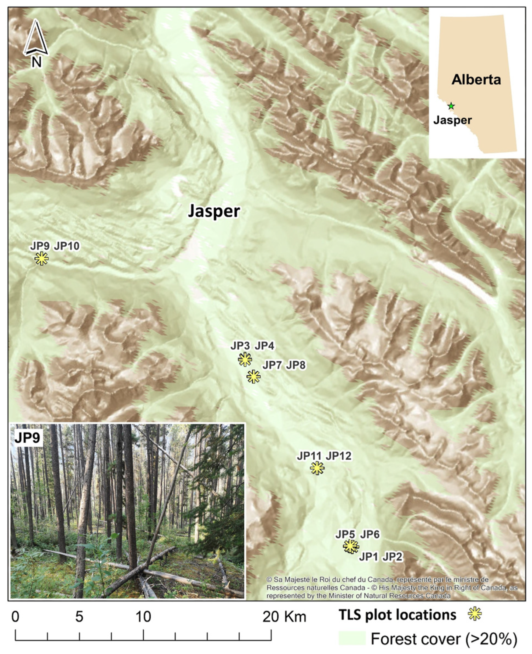
2. Study Area and Data Collection

Our study site is located near the tributary basins of the Athabasca River and Miette River within the eastern main ranges of the Canadian Rockies in Jasper National Park (Figure 1). The elevation of the valley basins ranges between 1050 and 1200 m with a typical annual average temperature of 4.1 °C. The predominant species in the park (and examined in the TLS and field plots) is Pinus contorta (lodgepole pine), categorized as fuel type C-3 in the Fire Behavior Prediction (FBP) system. A decade long attack of mountain pine beetle (MPB) has altered the existing fire regime by dehydrating and often killing many of the pine trees, causing the transition from healthy green trees into the red-phase, where needles have died but remain on branches (and are red in color), and grey-phase, where needles have dropped from trees, leaving remaining grey branches on the trees and causing the accumulation of dry woody debris on the forest floor. This region is characterized as a lightning-shadow area with a low flash density of less than 0.5 per km2 per year [74]. The majority of lightning events occur during the night-to-morning period near water bodies, which is atypical of severe lightning commonly associated with local solar heating for thunderstorms [75]. However, studies have indicated that the eastern aspect of terrain features within the elevation range between 1200 and 2000 m could enhance flash density [75,76], consequently increasing the risk of fire occurrence and subsequent spread into adjacent valley basins. The accumulation of fire fuels from mountain pine beetle and drying potential is also of significant concern for the town of Jasper, which is also located at the confluence of the basins (Figure 1). This was exemplified in September 2022 when a fire occurred 15 km north of the town of Jasper, reinforcing the importance of fuel monitoring, prescribed fires, and fire prediction in the area.
Twelve adjacent TLS plots coincident with the field data were collected at six locations along the valley south and west of the town in July 2021. Two plot centers were located side by side at a distance of 40 m to reduce movement of the TLS and to increase sampling efficiency at each location (Figure 1). A Teledyne Optech Polaris TLS station (1550 nm) was placed at each plot center for a 360° × 120° scan and at four corners 20 m from the plot center to complement the central scan and reduce the occlusion of returns. TLS scans were collected at a rate of two plots per day. Trees within an 11.3 m radius from each plot center were also measured for their species, tree height, diameter-at-breast-height (DBH), live crown base height (LCBH), dead crown base height (DCBH), tree phases under MPB attack, and the approximate degree of dead condition (Dead %). A tree with a Dead % value of 100 characterized a leaf-off tree. A total of 572 trees were surveyed including six major species: lodgepole pine (Pinus contorta), white spruce (Picea glauca), black spruce (Picea mariana), trembling aspen (Populus tremuloides), Douglas fir (Pseudotsuga menziesii), and subalpine fir (Abies lasiocarpa). The selection of twelve plots represented a wide range of fuel conditions with varying stem density, terrain slopes, sub-canopy thickness, and tree health (Table 1). Individual trees were not geolocated due to time constraints. Instead, plot quadrants were separated by four cardinal directions and tree locations within quadrants were visually identified. Figure 1 shows an example ground-level view of the JP9 plot in which ladder fuels and downed woody logs are prevalent in the plot.
For each scan, a point cloud was generated using all laser returns, incorporating an intensity attribute for each point. Point clouds of corner scans from TLS were co-registered manually based on the 3D tie points with CloudCompare (v2.11) [77]. The selection of tie points are iterative trial and error based on the sharp branch edges until no obvious visual displacement is found. A plot consists of 7–10 tie points spread over different corners. The co-registration error was represented by the root-mean-square error of all tie points in the plot from CloudCompare. The registration errors per plot are summarized in Figure 2 with an average error of 1.9 cm. It is worth noting that in situ targets are commonly preferred for achieving optimal registration accuracy. These were excluded from this study due to the inefficiency associated with their setup and their limited discernibility in plots rich with understory vegetation. All registered scans were merged into a single ‘plot’ point cloud, cropped to a circular radius of 25 m, and then resampled to a spatial resolution of 5 mm for further processing. A spatial resolution of 5 mm was specifically selected as it provides a reasonable balance between the ability to discern branches from noise conifer trees and computational efficiency for subsequent analyses. TLS plot scans were georeferenced to point clouds acquired from airborne laser scanning (ALS) collected the same summer (early August, 2021). The georeferencing followed a similar manual registration procedure as that employed for TLS co-registration. Iterative selection of 10–14 tie points was performed on the tree tops and crown edges from both the TLS and ALS datasets until visual overlap of the crown shapes was achieved. The mean error associated with this TLS-to-ALS georeferencing process was determined to be 24.8 cm.

3. Methodology

3.1. Workflow and Preprocessing

The primary workflow decomposed TLS point clouds into eight classes, which are important for quantifying fuels: tree stems, tree branches, tree foliage, seedling stems, downed woody logs, below-canopy branches, ground points, and other non-wood foliage and litters (Figure 3). Within this classification scheme, below-canopy branches refer to non-stem wood points with diameters greater than 5 cm within the saplings, shrubs, and surface layers. Ladder fuels are further differentiated into categories such as leaning trees, below-canopy dead branches, and downed woody logs. Within the scope of this paper, these leaning trees and stems are respectively referred to as “ladder trees” and “ladder stems”. It is worth noting that some dead fallen trees may not make contact with the ground but could possess a moderate leaning angle. From our observations, such instances are relatively infrequent. We identified downed woody debris based on a high inclination angle exceeding 60° as this criterion clearly demarcates the boundary between the leaning tree layer and the downed woody debris layer. Varying classifiers and filters were used to extract the class of interest for each point and the eight classes were combined and used to form a multi-class point cloud per plot. The classifications were programmed using PyTorch (v1.13), Python, and all the remaining processes using MATLAB (R2022b). PC configuration included an Intel® Core™ i7-12700K 12 × 3.60 GHz, 128 GB RAM, and NVIDIA GeForce RTX 3090 (24 GB).
The subsequent post-classification scheme is illustrated in Figure 4. Individual tree components such as stem, branch, and foliage were clustered. Wood was reconstructed into cylinder-shaped 3D architecture models using a custom QSM model. All other coarse wood components were isolated and reconstructed to estimate the wood volume across each plot.

3.2. Classification of Tree Point and Coarse Wood Components

The major components, namely, tree, stem, and downed woody log points were extracted using a state-of-the-art deep learning classifier SegFormer [78] customized in a 3D voxel version (Figure 5a). The definition of trees in this study did not include saplings with a height < 5 m. SegFormer replaces the classic convolutional neural network (CNN) layers with self-attention-based transformers, surpassing well-recognized semantic classifiers such as DeepLab V3 [79] and Swing Transformer [80] in terms of an overall rating of computation efficiency and accuracy. The SegFormer parameter values remained set to default and its configuration of voxelization, sampling, training, and testing followed the scheme in Xi et al. [71] except for the block size and voxel resolution (Table 2). A block of voxels was the input unit to the SegFormer. The block size was selected as 128 × 128 × 128, which maximally exploited the GPU RAM capacity. The voxel resolution was customized based on the scale of interest: for example, smaller features such as downed woody logs matched a finer classification resolution (Table 2). The laser intensity was appended to each voxel as an additional layer to enhance the detection of coarse wood (stems and downed woody logs). Four plots with manually delineated tree and non-tree classes were used as the training sample (Figure 5b) with another single plot used as the independent testing sample. It was manually intensive to label wood and non-wood points as the training and testing reference over entire plots. Therefore, a subset of the plot scan with a size of ~8 × 8 m2 was clipped. A total of 10 and 21 clips (or subsets) were created from the TLS scans to train the classifiers for the stems (Figure 5c) and downed woody logs and branches (Figure 5d), respectively, along with two and three clips for testing. A training block was randomly located within each random clip and was also rotated horizontally by a random degree. This was considered as a data augmentation process to mitigate overfitting under a small sample size. The accuracy evaluation metric was the mean inter intersection over union accuracy (mIoU). Incorrectly classified points were edited and cleaned for the wood isolation and tree clustering processes.

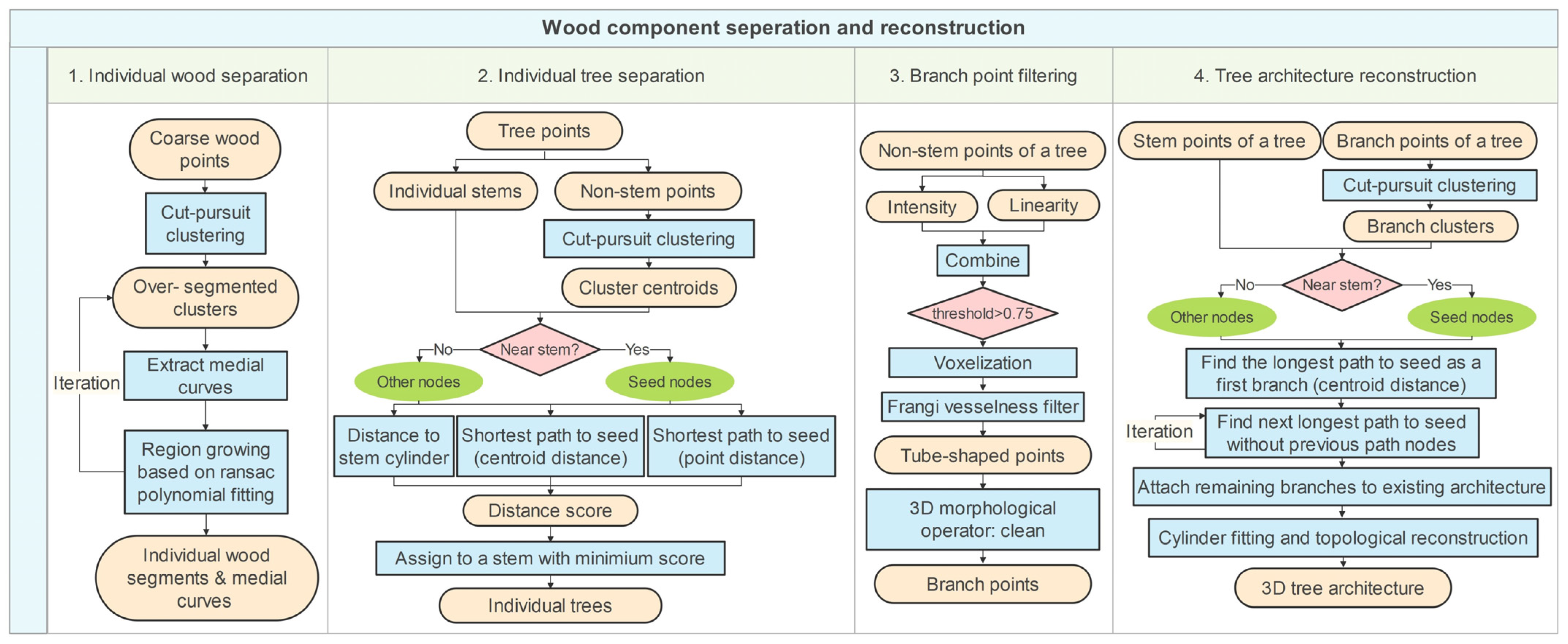
3.3. Individual Wood Isolation

The classified stem points inevitably contained small isolated fragments detectable using the connected component analysis [82]. Any connected fragment with a length or width < 5 cm was considered as noise and discarded. The remaining points were then clustered into small segments using an l0 cut-pursuit algorithm [83]. The cut-pursuit algorithm has two main parameters: the number of neighbors (K) from the nearest neighbor search as the minimal unit, and the regularizer λ as the overall graph scale [69]. The greater the K and λ set, the coarser the clusters that would be generated. Both were set to 20 in this study, and the resulting clusters were mainly sized between 0.1 and 10 m. Due to stem occlusions in the crown area, these clusters did not encompass the complete stem components and required merging.
Clusters were sectioned at 0.1 m intervals along their principal directions, as determined by the first component of principal component analysis (PCA). These sections captured the general shape of each cluster. A region-growing method was developed to merge clusters belonging to the same stem, representing a cluster by a sequence of its slice centroids. The nearest pair of clusters was tentatively combined and fitted with a 3D third-order polynomial curve. If the curve fitting error fell below a threshold, these clusters were merged. These steps were repeated for the remaining clusters until no suitable fitting was found. In practice, noise and adjacent stems could lead to incorrect curve fitting such as the lower part of one stem merging with the upper part of neighboring stems. To enhance the robustness of the 3D polynomial curve fitting and prevent over-merging across stems, a RANSAC selection scheme was employed, rejecting outlier centroids. The criteria for “goodness of fit” of the points along the curve were represented by the smoothness and consistency of the points surrounding the curve. The smoothness, represented by the absolute median deviation (MAD) between the fitted curve and slice centroids, should be less than 30 cm (corresponding to the maximum stem cylinder radius in this study). When fitting a pair of clusters, the median deviation of the curve fitting for one cluster was compared to that of the other cluster. The resulting ratio, which represents the curve-fitting consistency between the two clusters, was constrained to be less than 4. Depending on the practical situation, this ratio could be set more stringently such as 3. The RANSAC-based region growing merged well-fitted clusters iteratively until smooth and consistent stem curves were segmented from the stem classification points. The same method was applied to segment the downed woody logs into individual components.

3.4. Individual-Tree Clustering

In the study plots, it is common for trees to be densely packed and occasionally intersect with inclined ladder woods. Conventional individual-tree segmentation, based solely on point density, may underestimate fuel levels in areas where trees overlap or cluster together. Our method adapted the simple morphological rule that a tree stem forms the base for branch and foliage attachment. Among the classified trees, points were segmented into individual stem and non-stem points. The latter were transformed to the cluster scale using the cut-pursuit algorithm described above, but at a finer spatial resolution (K = 5, λ = 1). This resolution matched the typical size of branch and foliage clusters, where each cluster defined a graph node N . The non-stem clusters were assigned to the nearest stems based on a closeness measure adapted from the method by Wang [58]: (1) any non-stem nodes within 10 cm of the stem points were considered ‘seed nodes’ ( N s ), while other nodes were considered to be ‘non-seed’ nodes ( N n ); (2) the shortest path ( L m i n ) to each seed node N s was calculated for each N n using Dijkstra’s algorithm [84]; (3) two distances ( D c and D p ) along the shortest path L m i n were calculated for each N n , where D c was determined by the accumulated distance from the centroid of N n to the centroid of N s , and D p by the accumulated 3D point gaps from the point cloud of N n to the point cloud of N s , respectively; (4) the projected distance D m between N n and the medial line of N s was calculated; (5) a distance score, defined by a weighted average of the three distances D c , D p , and D m , was determined as the closeness measure; (6) an N s was clustered to the N s with the minimum score, and both were assigned with the ID of the stem nearest to the N s . The weights of D c , D p , and D m , defined as 0.4, 0.3, and 0.3, respectively, were customizable but did not require lengthy optimization for satisfactory individual-tree clustering. In practice, individual stems from previous steps could contain errors. A typical error is the misclassification of thick branches in the crown as a stem and isolated as an incorrect stem in the classification. Our amendment was to repeatedly merge two individual trees if the bottom of one tree fell above the top of the other tree with a projected horizontal overlap of >80%. Overall, individual trees were isolated using the shortest-path and conditional merging rules.

3.5. Branch Classification

A similar deep learning model for branch classification is also feasible, however, creating sufficient branch references to train deep learning from fuel-rich plots is laborious and impractical. Furthermore, human-interpreted thin branch samples can be erroneous and difficult to identify within a dense and crowded canopy. This study proposed an alternative solution to deep learning, circumventing the dilemma of reference making while potentially achieving a similar level of accuracy compared to the branch filtering accuracy of 0.54 reported by Xi et al. [85].
Ideally, branches are linear geometrical features detectable using a linearity-based filter. The linearity metric can be derived from PCA components [71]. The challenge is the weak signal of smaller diameter branch points surrounded by foliage and shrubs. The point clouds of larger diameter branches might also become fragmented and indiscernible due to the high occlusion of points by objects closer to the TLS. In this situation, the geometric identity of a branch can diminish, but its spectral identity remains visible, characterized by the intensity of laser returns [86]. The intensity alone, however, is not a robust indicator of branches when there are other environmental factors that influence the return intensity (e.g., local surface ruggedness) [87]. Therefore, a weighted-linearity-intensity index (WLI) combining the return intensity and the linearity of the branch was adapted in this study (Equation (1)):
W L I = w × s i g m o i d L i n e a r i t y + s i g m o i d I n t e n s i t y ,
Here, a weight parameter w was used to leverage the importance of either term, which was set to 1.0 for simplicity. Approximate branch points were classified using a WLI > 0.75.
Despite this initial filter, the classified branch points were still noisy. A Frangi vesselness (FV) filter, which is used in multi-scale vessel detection from 3D X-ray medical images [88], was adopted to enhance the branch pattern. In this study, the filtered point clouds were voxelized at a resolution of 1.5 cm. Five levels of scales (2, 4, 6, 8, and 12 times voxel resolution) were input to the FV filter corresponding to the range of branch thicknesses between 3 and 18 cm. A 3D voxel morphological operator was then used to remove the isolated blank voxels surrounding them. Branch points were then filtered within each individual tree. Ten pine trees within the twelve plots were manually cleaned and delineated based on the results of branch filtering as the validation reference. It is important to note that while the WLI, noise filtering, and QSM branch delineation collectively contributed to mitigating the noise issues associated with branch identification solely based on intensity, they did not fully address the attenuation of intensity signals caused by the distance and angle incidence. While multi-scan co-registration alleviated the attenuation effect, the inclusion of intensity calibration is expected to further optimize the accuracy of branch detection.

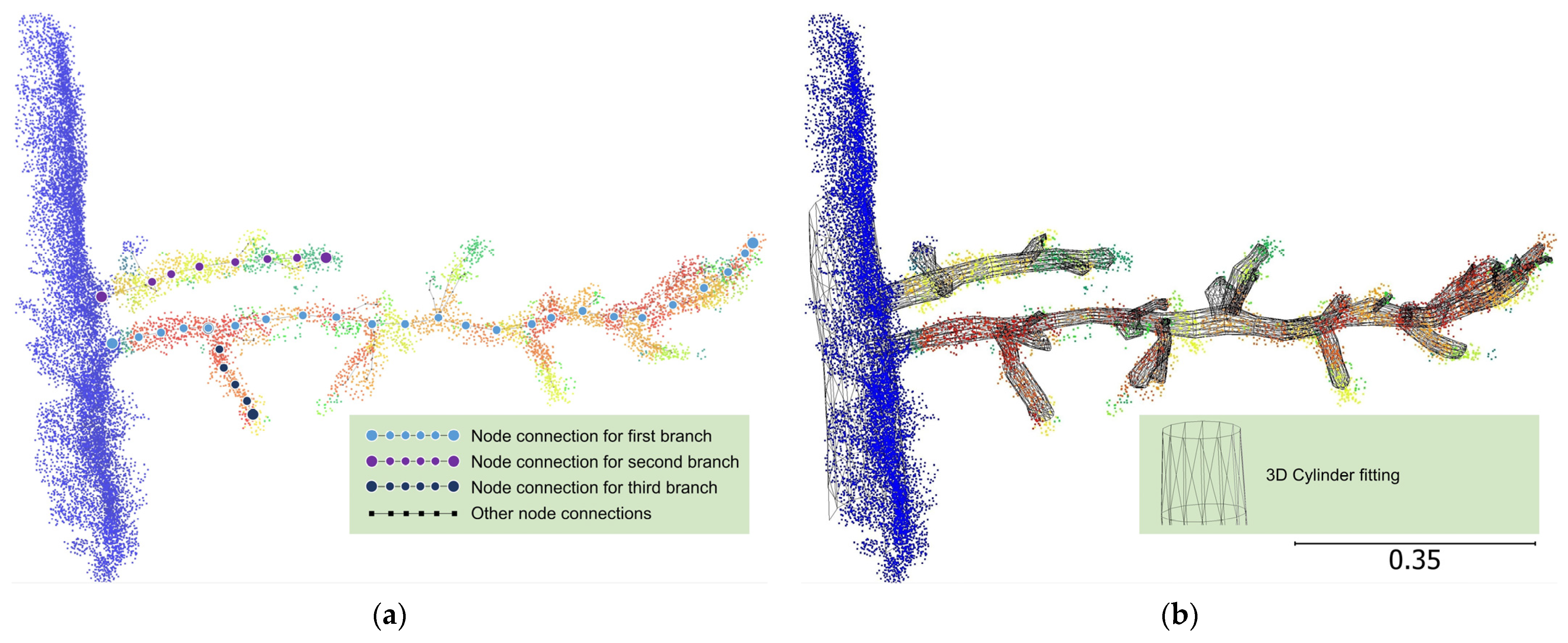
3.6. Tree Architecture Reconstruction

Tree architecture reconstruction, also known as QSM, not only includes the 3D geometric modeling of branches and stems using cylindrical proxies, but also the establishment of the topologic relationship between wood components. Each individual branch requires isolation and to be subsequently arranged in a hierarchical order, beginning with the main branch connected to the stem, followed by the smaller branches attached to it, and continuing in this manner. This is achieved in a similar manner to the tree clustering approach (Section 3.4). Here, branch points are first clustered using the cut-pursuit algorithm. Branch clusters near stem points are considered as seed nodes. The shortest paths from the remaining nodes to the seed nodes are generated with a maximum point gap between two clusters of 3 cm. The shortest path with the greatest accumulated distance is classified as an individual branch, and all nodes along this path become branch nodes. As an example, Figure 6 demonstrates that the parent node of a branch is the stem node closest to the first node of the path. Likewise, nodes along the path with the next greatest accumulated distance form the second branch. The second branch discards any nodes already belonging to other branches, where the parent node is the joint node (i.e., the last node of the discarded part) of the previous branch. The branch generation process is repeated until no close clusters (gap < 3 cm) are found. The remaining isolated clusters with a gap between 3 and 30 cm are further attached to the existing branch architecture using the same shortest path rule, except that the seed nodes are closest to the existing branches instead of to the stem. Remaining isolated clusters are discarded. All individual branches are fitted with a sequence of circles [89] every 10 cm (customizable) using least-square minimization, which determines the branch direction and radius at each segment [85]. The branch radii occasionally encounter large values due to the inclusion of locally noisy points included in the circle fitting algorithm. To address this issue, the impact of outlier points on the branch radius was reduced using a moving-window median filter along each branch, employing a maximum cut-off value based on the median of all branch radii and a minimum cut-off value of 2.5 mm for the branch radius. This approach mitigated the problem of volume overestimation for small branches with diameters < 5 cm as reported by Demol et al. [90].

3.7. Fuel Attribute Extraction and In Situ Validation

The above-described classifications of specific plot components such as stems and branch points are not mutually exclusive. Some points can be associated with more than one class. Consequently, an additional step was needed to synthesize the classes and prevent ambiguous one-to-many class mappings. Specifically, the tree, within-tree stem, branch, and foliage classes were labelled with class 1, 2, and 3, respectively. Non-tree points mainly included subcanopy shrubs, sapling layers, and surface grass. From the viewpoint of fuel analysis, these points were treated as a whole without the individual segmentation used for individual trees. Point clouds of downed woody logs within the non-tree class were assigned class 4. Stems and branches detected within the non-tree class represented sapling stems (class 5) and branches of seedlings and shrubs (class 6), respectively. The elevations of the lowest points per 3 × 3 m2 area of the non-tree class were extrapolated into a plot-size grid as a digital elevation model (DEM). Any points within the 20 cm buffer of the DEM were filtered as ground points including litter and surface grass (class 7). The remaining points presented tall grass and any below-canopy foliage (class 0). The class labeling followed a priority order to avoid ambiguity: class 1 > class 2 > class 3 > class 5 > class 4 > class 7 > class 6 > class 0.
This multi-class plot delineation enabled the fine-scale attribute extraction of separate fuel components. The stem tilt angle (TA) was quantified using the third coefficient of the first principal component of the stem point clouds from the PCA analysis. Ladder stems (including stems from shrubs and saplings) were filtered from individual stems with a TA > 10°. The ladder stems with any attached branches constituted ladder trees. The live crown base height (LCBH), which was measured in the field, was approximated based on the height of a point with the maximum curvature along the height-specific voxel volume profile, in other words, the knee point or inflection point similar to Popescu and Zhao [91]. Branch and stem volumes were determined as the total volume of 3D fitted cylinders from the QSM model described in Section 3.6. At the plot level, it is difficult to reconstruct complete geometries of downed woody logs and branches near the ground and in the duff layers of the soil due to the high occlusion of returns and complex shapes. The volumes of these components were inferred based on the linear relationship between the voxel volumes of the stems and branches, namely, SVOL and BVOL, and their QSM volumes of the counterparts, namely, QSVOL and QBVOL.
In situ measurement of tree heights, DBH, and LCBH were used to partly validate the accuracy of the diameter and length extraction from the delineated plot components using TLS. RMSE and Pearson’s r were used as the accuracy metrics. DCBH, while measured, was not used here due to the interpretation of what constitutes the height of dead branches vs. live ones (as a proportion), and therefore there is measurement uncertainty due to the vision occlusion from the under-canopy and shrub layers. Measured trees from each field quadrant (separated by cardinal coordinates) were manually linked to the isolated TLS trees based on tree orientation, DBH, LCBH, species, and tree height.

4. Results

4.1. Classification, Segmentation, and Filtering Accuracy

The SegFormer tree classification is visualized in Figure 7 with trees in red. Large variations in the tree distribution pattern and density were observed in the classified tree points due to time since post mountain pine beetle attack (and phase). JP8 had the visually sparsest tree distribution and JP9 the densest, also observed in the stem density survey in Table 1. A species mixture of mature pine, fir, and aspen was also observed in JP5 and JP6, and fir saplings were visible in JP7, JP8, JP11, and JP12. The crown apices of fir saplings were prone to misclassification as trees (e.g., in JP 8 and JP11) due to their intermediate height. Note that the intent of tree classification might be identical to the ground removal scenario [67] where algorithms such as the cloth simulation filter (CSF) [92] abound. The subtle difference is that a tree classifier needs to identify tree points from the subcanopy complexes instead of simple height slicing using the ground DEM buffer (e.g., CSF). The stem bottoms within the DEM buffer need to be preserved as the stem class. Deep learning addressed this complexity, yielding a high mIoU accuracy of 0.91 from four testing plots (Table 3).
The stem point classification was contrasted with the reference in the example JP9 clip in Figure 8. The SegFormer could identify most stem points with slight over-detection: major stems were thickened, and additional linear shapes in the crown were misclassified as stems. The former edge issue could be caused by the setup of a slightly coarse voxel resolution of 4 cm and the latter inscrutable noise is a common issue of deep learning [93]. The challenge was to detect sparse stem signals within dense, needle-leaf fir crowns where existing studies either excluded the classification of fir species or demonstrated insufficient accuracy [94], however, for wildland fire, fir is an important species because it is highly flammable. These issues were mitigated in Figure 8, where the mIoU of the fir stem classification was 0.89, and the stem classification over all testing samples was 0.94 on average (Table 3). The example classification results of downed woody logs are also visualized in Figure 8. SegFormer tended to detect outlying small, round-shaped pieces of wood in addition to the reference ones. Using the manual reference as the baseline, the mIoU of woody log classification was 0.81. Figure 8 also shows the example of stem and downed woody log classification over JP1. From the birds-eye view, not all coarse woody log points from the reference were captured by SegFormer, especially among the oblique stems and highly-occluded thin ground logs. This issue partially arose because the manually created training samples did not represent sufficient instances of oblique or highly-occluded woody logs, and the deep learning model was not adequately trained to handle such intricate situations. While increasing the representation of these complex instances in the training dataset could potentially address this issue, such an approach would require further manual editing, a resource-intensive task that was beyond the scope of this study.
The example results of cut-pursuit clustering and individual wood isolation are illustrated in Figure 9 using a JP2 clip as an example. The classified stem points were manually cleaned before the clustering and isolation. Small stem clusters with linear shapes were generated by cut-pursuit and further merged into complete wood segments using the RANSAC-based region growing method. Some bending and occlusion (Figure 9c) could be overcome due to the polynomial fitting of the RANSAC method. The intersection of two or more stems or downed woody logs, a typical barrier for correct segmentation, can also be addressed to a certain extent using our method. Issues with the segmentation included the failure of merging several small irregular or highly curved clusters. Plot-level tree clustering based on individual stems is illustrated in Figure 9d–f using JP1 as a second example in this figure. The classified stems were uncleaned, resulting in an issue of over-isolation (Figure 9e), where more stems were isolated than actually exist. This could be mitigated by the use of overlap-based merging during tree clustering (Section 3.3) (Figure 9f). Many trees that were intersected in the crown could be separated with well-delineated boundaries due to the morphology-based shortest path rule (Figure 9f). Accuracy assessment did not include incomplete and sparse trees near the edge of the plot caused by the partial scan coverage. The mIoU of stem isolation and individual tree clustering was 0.73 and 0.86, respectively.
The branch processing and classification results are shown in Figure 10. The WLI index, which integrates the intensity (Figure 10a) and linearity (Figure 10b), filtered out dense foliage (Figure 10c, without stems), and the FV filter smoothened and enhanced linear shapes (Figure 10d). Figure 10c also reveals that a fraction of the twig points was also filtered out, which can underestimate the fuels available for fire as these burn more readily than larger diameter branches. There was a tradeoff between the partial loss of branch points and the need to exclude foliage and noise points from the classification. The plots in our sites consisted of mostly mature, high foliage trees, which also contributed to a high level of return noise. Therefore, a high threshold of 0.75 was set for the WLI, leading to the filtering of branches from fine branch material and needles. Using our testing reference, branch filtering had an mIoU of 0.62.
Following the synthesis of classifications into eight classes, the fine-scale composition of a plot could be represented, as demonstrated in detail for a small area of the JP7 clip (Figure 11a) and across the larger plot using JP1 (Figure 11b). It is evident that foliage in the dark green color (class 3) was primarily distributed among fir trees, short pine trees, and the lower portions of tall pine trees in JP1. Occlusion occurred mostly near the plot edges and on the ground near the corner TLS stations. Understory grass and herbaceous layers indicated by light green (class 0) tended to have an overstory of large crown diameter trees or tree clusters, which enhance shading and reduce water loss, while large spaces between trees had shorter/less dense grasses and was primarily represented by ground returns. The horizontal orientations of ladder trees appeared randomly distributed.
The complete QSM reconstruction at the tree- and plot levels is presented in Figure 12. Results of the branch clustering based on the shortest path rule, skeletonization, and cylinder-fitting are illustrated in Figure 12a–c, respectively, based on the same point cloud in Figure 10 (JP7) and the 3D wireframes from QSM reconstruction (Figure 12d,e) based on the point clouds in Figure 11 (also for JP7). Here, narrow branch diameter branch structures were also captured by the 3D reconstruction. A notable issue was the exaggeration (or artificial increase) in the reconstructed stem diameters near the apex of the tree crown due to the noise points during the circle fitting.

4.2. Field Validation

A total of 269 trees with field measurements were matched to isolated TLS trees within the twelve plots. From these, a subset of 84 trees had live crowns, which was used to calculate LCBH. The r2 between the field measurements and TLS extraction was 0.95 for tree height, 0.96 for DBH, and 0.60 for LCBH, respectively (Figure 13). RMSE (RMSE%) was 1.3 m (9.0%) for tree height, 1.3 cm (8.7%) for DBH, and 2.6 m (39.6%) for LCBH, respectively. The bias of TLS height, DBH, and LCBH was −0.53 m (−3.8%), 0.54 cm (3.5%), and −0.35 m (−5.3%), respectively, compared to the field measurement. TLS tended to underestimate the LCBH. The differences are algorithm- and species-specific, and are not consistent among the different studies that have used TLS [95,96].
When comparing the QSM approach for volume calculation, the wood volume determined by counting voxels was subject to the choice of voxel size and the completeness of the scanned surface. Utilizing a voxel size equal to the point cloud resolution of 5 mm led to the underestimation of individual tree wood volume by 81% (branch)–92% (stem), respectively, compared to the wood volume derived from QSM reconstruction. Increasing the voxel size might mitigate the underestimation but would introduce complexity in adjusting the voxel size for different tree and plot components. A linear relationship between these two volumes was observed excluding minor extreme outliers (Figure 14). The r2 was 0.54 between SVOL and QSVOL from all individual trees, smaller than the r2 of 0.95 between BVOL and QBVOL. The diameter of stems was mostly greater than 5 cm, and simple voxelization of stem surface points did not account for the volumes within the stem body. Conversely, branch diameters were smaller with many contained by voxels, causing better agreement between the voxel and QSM volumes.

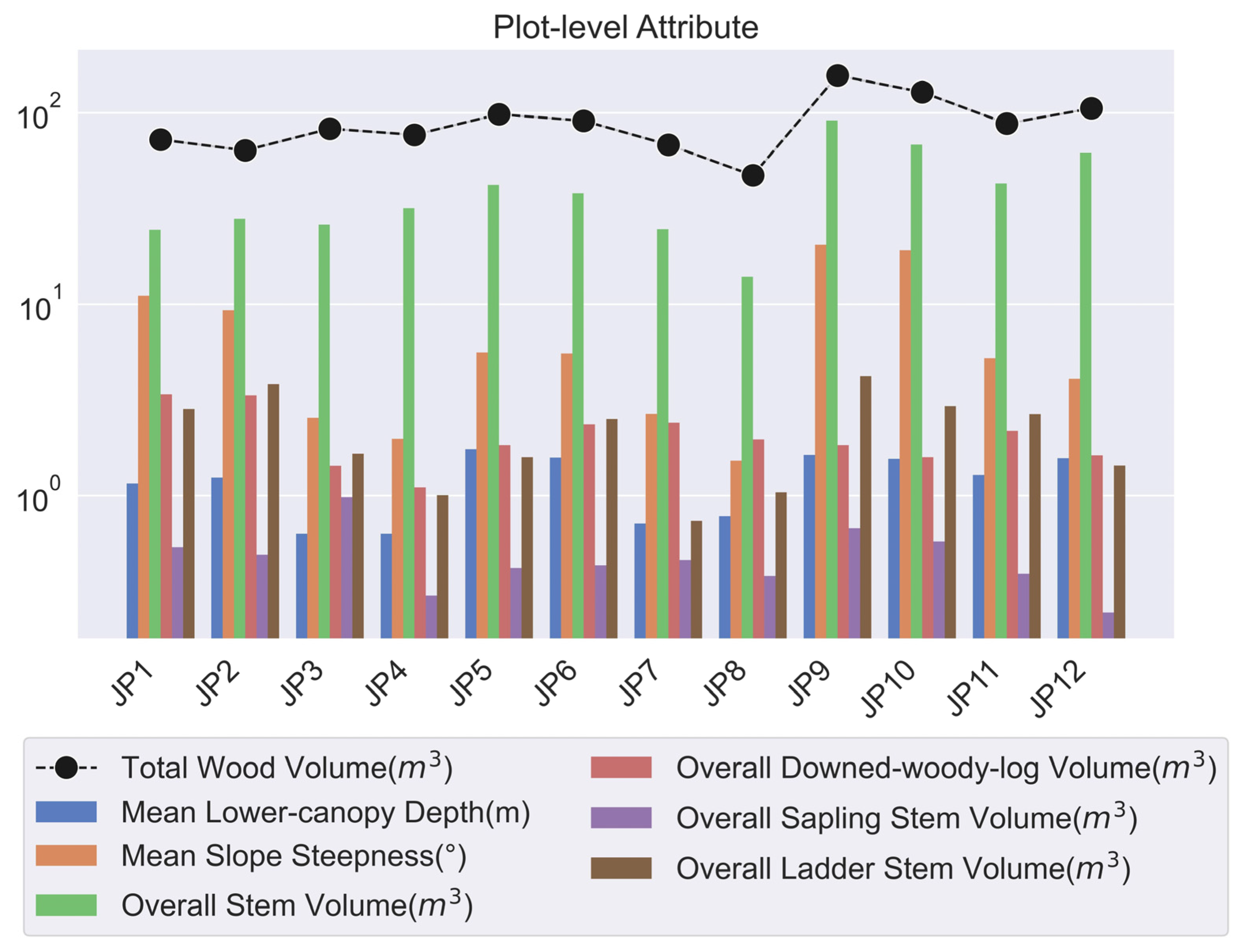
4.3. Plot-Level Attribute Analysis and Volume Calibration

At the plot level, the downed woody volume, sapling stem volume, and ladder stem volume were scaled from the voxel volumes based on the ratio of QSVOL to SVOL, and the below-canopy branch volume and ladder tree branch volume based on the ratio of QBVOL to BVOL. The result component volumes and other plot-level attributes are provided with a summary chart in Figure 15. Except for JP12, which was heavily affected by MPB, JP9 and JP10 had the highest concentration of stem to the total plot volume (58.3% and 53.2%, respectively) in the steepest slope (mean slope angle = ~20°), and the lowest branch volume proportions to the total tree volumes (19.5% and 23.3%, respectively). This aligned with the visual appearance in Figure 7 that trees in JP9 and JP10 were dense and straight but with narrow individual tree crowns. JP5 and JP6 presented another distinct plot configuration: mixed species (pine% = 65–75%, fir% = 13–16%) and a thick sapling layer (~4% of the total plot volume compared to the average of 2% among other plots). However, the concentration of ladder tree volume in both plots remained at an average level compared to other plots. In contrast, JP7 and JP8 had only four ladder trees and few saplings. JP8 had the lowest wood volume concentration (60.7%). JP1 and JP2 had the highest ladder stem volume (4–6% compared to the average of 2% among other plots). The ladder stem volume was strongly associated with stem density (r = 0.85), existing straight stem volume (r = 0.49), and DEM slope (r = 0.81), indicating a positive effect from competition and gravity factors. The vertical distributions of each fuel component with slope correction are visualized as stacked area charts in Figure 16. It can be seen that the plot-level composition varied significantly with geographic locations but remained similar between neighboring plots. The stem volume distribution mimicked a Weibull curve, descending at a faster rate toward the tree top than the branch volume distribution. The vertical distribution of foliage volumes was similar to that of branch volumes. Ladder fuels and saplings contributed to a negligible proportion at the plot level in terms of tree volumes in Figure 16. In most plots (JP2, 3, 7, 8, 9, 10, 12), a boundary existed between the tree branch layer and the below-canopy branch layer. The presence of a ladder tree layer between them created a noticeable connection between the two potentially combustible layers. The average overlapping area of the vertical volume profile excluding the ladder tree layer was 8.4% relative to the union area of the tree layer (stem, branch, foliage) and the below-canopy layer (all other components). Including the ladder layer, the overlapping degree increased to 10.8%.

5. Discussion

The study of forest component classification from TLS has gained prominence in the research community over the last decade. Among the available methods, many geometric algorithms have demonstrated excellence in stem detection [97,98,99,100] and wood and foliage classification [70,101,102,103], which are alternatives to the emerging deep learning solutions [71,85,104]. However, the limitations of this method are also obvious, whereby rule-based algorithms are too specified to be adaptive to complex environments, which include standing and ladder trees, saplings, and downed woody logs. In comparison, deep learning classifiers can exhibit flexibility without sacrificing accuracy. In this study, SegFormer was employed as a binary classifier (e.g., tree vs. non-tree, and stem vs. non-stem). Altering SegFormer to function as a multi-class classifier, which simultaneously classifies stems and downed woody logs together, resulted in a reduced accuracy. The mIoU decreased by 0.05 (6%) to 0.82 compared to the average mIoU of 0.87 when classifying these components separately. This finding coincides with a recent study by Li et al. [105] where binary CNN-based classifiers exceeded the multi-class situation in wetland vegetation classification with an mIoU increase by 22%. However, the processing time would significantly increase if each class is trained individually.
In addition, deep learning was not used for branch classification due to the low efficiency of branch sample delineation from dense conifers. The detection of fine branches in spruce remains an issue. The geometrical algorithm developed by Hui et al. [70] has demonstrated overall superiority in branch filtering, with the exception of narrow spruce branches. The filter in our study could detect twigs but also contains cones and some noise as a function of the point cloud distribution. Several tree species such as the subalpine fir and Douglas fir were not widely sampled within the training data but coexisted with other conifers found in the plots, adding to the uncertainty of the stem classification. In addition, one stem per tree was the underlying assumption of our stem isolation algorithm, which could be violated by the “co-dominant stem” strategy where two leader stems grow from single trees to withstand environmental stressors [106]. This phenomenon was found occasionally within plots and could potentially result in the underestimation of the true stem volume. It was also observed in the field that dead pine trees in grey phase following mountain pine beetle attack retain some mosses and lichens on the branches. Lichens could be mistaken for foliage from TLS without field validation [107] and may increase return classification biases to increase the branch volume.
The result RMSE% of tree height and DBH in Figure 14 fell within the average range of 13–30% and 5–15%, respectively, a common range from a benchmarking study on eighteen contemporary methods in 2018 [108]. Tree heights were underestimated by TLS (Figure 14), as also observed in other studies [95,108]. The near-zero biases of the TLS DBH aligned with studies [108] using similar extraction methods. Compared to the height and DBH, the TLS LCBH had weaker correspondence with the field measurement. Causes could be an unclear definition of LCBH from an abnormal crown shape, especially the unhealthy trees [109], and the fallible measurement of crown bases from heavily overlapped crowns [110]. From the literature, the former cause was insignificant regarding the strong r2 (>0.9) between the human-interpreted and the automatically extracted crown base height (CBH) from TLS by Seidel et al. [111]. The field measurement error of CBH was considered the main issue [112]. The literature with TLS CBH validation is rare due to the strenuous efforts of obtaining CBH from the field [112]. Among the available studies, Jung et al. [110] reported a high r2 of 0.82 but had a limited validation sample size of fifteen trees. Fernández-Sarría et al. [113] validated the LCBH accuracy with thirteen field trees and reported an r2 of 0.52, in line with this study. A stand-level assessment of CBH accuracy was conducted by Pyörälä et al. [114] with a relatively lower validation r2 of 0.20. All of these studies demonstrated a significantly stronger r2 from the height and DBH validation compared to CBH, indicating a reliability issue of field mensuration to determine CBH.

6. Conclusions

The capability of TLS has facilitated the enhancement of our understanding of fuels within forests, from landscape- and stand-based scales to a more nuanced focus on individual trees and branches. While TLS is gaining wider application in fire fuel studies as a replacement for inventory mensuration, it is primarily based on voxel profile information, without the in-depth incorporation of advanced data processing and AI techniques. An analysis of the fine-scale forms of trees and branches based on AI methods provides a more detailed understanding of the intricate nature of forest fuels and their connectivity, which may be further assessed along with local climate including the drying potential. This study broadens the extent of existing TLS investigations to characterize fuel components at the plot scale based on deep learning, incorporating ladder trees, fallen woody logs, subcanopy branches, and surface layers. Twelve TLS plot scans were collected from a C3 fuel type with lodgepole pine that were, in many plots, at various stages of mountain pine beetle attack and mortality. The TLS extraction of tree height, DBH, and LCBH matched the in situ mensuration, while TLS provided additional detail of the volume distribution of each plot component along the vertical height. This scheme of component division could help refine the fuel load quantification among materials with different flammability and also indicate the vertical continuity of different fuel components. The existence of a ladder tree layer enhanced the overlap degree between the two combustible layers of individual-tree branches and below-canopy branches from 8.4% to 10.8%. In addition, a significant underestimation of wood volume based on conventional voxel-based counting at fine resolution was found compared to the more reasonable QSM method due to scan occlusion. It is suggested that QSM is applied to calibrate voxel-based wood volumes for fine-scale fuel analysis.
The differentiation of forest components serves as a foundational dataset for a range of fire-related studies. With respect to fire fuels, the grass and litter layer is associated with fine fuels, coarse fuels represented by individual-tree stems and downed woody logs, and intermediate fuel loading embodied by branches. The fraction, length (or height), and diameters of individual fuel components provide essential input in the allometric equations of fuel load [115]. Overall, the parameters of the wood components and terrain hold significance for the planning (e.g., prescribed burns), the potential for ignition, and the prediction of the fire rate of spread. The proof-of-concept in this study illustrates the bright future of TLS in accurately quantifying the fuel physical properties for wildland fire analysis.

Author Contributions

Conceptualization, L.C.; Methodology, Z.X.; Software, Z.X.; Validation, L.C.; Formal analysis, Z.X.; Investigation, L.C., C.H. and Z.X.; Resources, L.C. and C.H.; Data curation, Z.X.; Writing—original draft preparation, Z.X.; Writing—review and editing, L.C. and C.H.; Visualization, Z.X.; Supervision, L.C. and C.H.; Project administration, L.C.; Funding acquisition, L.C. All authors have read and agreed to the published version of the manuscript.

Funding

This research was funded by Mitacs Accelerate [grant number IT27605], the Foothills Research Institute (fRI)—Federal-Provincial MPB Research Partnership [grant number 247.15], NSERC Canada Wildfire [grant number SPG-N—NETGP 548629-19], the Canada Foundation for Innovation [grant number 32436], and Western Economic Diversification Canada [grant number 000015316].

Data Availability Statement

The reference TLS dataset is currently being published to the Federated Research Data Repository (FRDR) and can be accessed via https://doi.org/10.20383/103.0814 for long-term availability and maintenance.

Acknowledgments

Special thanks are extended to Tristan Skretting, Emily Jones, Saied Parsian, Linda Flade, and Viviana Lartiga for their invaluable assistance during fieldwork; to Chris Watson and Landon Shepherd of Jasper National Park for their field support and site access; to Jonathan Boucher from the Canadian Forest Service for his expert insights on fuel sampling; and to the Foothills Research Institute (fRI) and Mitacs Accelerate for their generous funding support.

Conflicts of Interest

The authors declare no conflict of interest. The funders had no role in the design of the study; in the collection, analyses, or interpretation of data; in the writing of the manuscript; or in the decision to publish the results.

References

  1. Liu, Y.; Stanturf, J.; Goodrick, S. Trends in global wildfire potential in a changing climate. For. Ecol. Manag. 2010, 259, 685–697. [Google Scholar] [CrossRef]
  2. Whitman, E.; Parisien, M.-A.; Thompson, D.K.; Flannigan, M.D. Short-interval wildfire and drought overwhelm boreal forest resilience. Sci. Rep. 2019, 9, 18796. [Google Scholar] [CrossRef] [PubMed]
  3. Jain, P.; Wang, X.; Flannigan, M.D. Trend analysis of fire season length and extreme fire weather in North America between 1979 and 2015. Int. J. Wildland Fire 2017, 26, 1009–1020. [Google Scholar] [CrossRef]
  4. Westerling, A.L.; Hidalgo, H.G.; Cayan, D.R.; Swetnam, T.W. Warming and Earlier Spring Increase Western U.S. Forest Wildfire Activity. Science 2006, 313, 940–943. [Google Scholar] [CrossRef]
  5. Coogan, S.C.P.; Daniels, L.D.; Boychuk, D.; Burton, P.J.; Flannigan, M.D.; Gauthier, S.; Kafka, V.; Park, J.S.; Wotton, B.M. Fifty years of wildland fire science in Canada. Can. J. For. Res. 2021, 51, 283–302. [Google Scholar] [CrossRef]
  6. Jain, P.; Castellanos-Acuna, D.; Coogan, S.C.; Abatzoglou, J.T.; Flannigan, M.D. Observed increases in extreme fire weather driven by atmospheric humidity and temperature. Nat. Clim. Chang. 2022, 12, 63–70. [Google Scholar] [CrossRef]
  7. Whitman, E.; Parisien, M.-A.; Thompson, D.K.; Flannigan, M.D. Topoedaphic and forest controls on post-fire vegetation assemblies are modified by fire history and burn severity in the northwestern Canadian boreal forest. Forests 2018, 9, 151. [Google Scholar] [CrossRef]
  8. Wotton, B.; Flannigan, M.; Marshall, G. Potential climate change impacts on fire intensity and key wildfire suppression thresholds in Canada. Environ. Res. Lett. 2017, 12, 095003. [Google Scholar] [CrossRef]
  9. Stocks, B.J.; Lawson, B.D.; Alexander, M.E.; Wagner, C.E.V.; McAlpine, R.S.; Lynham, T.J.; Dubé, D.E. Canadian Forest Fire Danger Rating System: An Overview. For. Chron. 1989, 65, 258–265. [Google Scholar] [CrossRef]
  10. Deeming, J.E.; Burgan, R.E.; Cohen, J.D. The National Fire-Danger Rating System—1978; Intermountain Forest and Range Experiment Station, Forest Service, US Department of Agriculture: Washington, DC, USA, 1977; Volume 39. [Google Scholar]
  11. Vitolo, C.; Di Giuseppe, F.; Krzeminski, B.; San-Miguel-Ayanz, J. A 1980–2018 global fire danger re-analysis dataset for the Canadian Fire Weather Indices. Sci. Data 2019, 6, 190032. [Google Scholar] [CrossRef]
  12. Van Wagner, C.E. Development and Structure of the Canadian Forest Fire Weather Index System; Canadian Forest Service, Forestry Technical Report; Government of Canada: Ottawa, ON, Canada, 1987. [Google Scholar]
  13. Woolford, D.G.; Martell, D.L.; McFayden, C.B.; Evens, J.; Stacey, A.; Wotton, B.M.; Boychuk, D. The development and implementation of a human-caused wildland fire occurrence prediction system for the province of Ontario, Canada. Can. J. For. Res. 2020, 51, 303–325. [Google Scholar] [CrossRef]
  14. Peterson, D.; Wang, J.; Ichoku, C.; Remer, L. Effects of lightning and other meteorological factors on fire activity in the North American boreal forest: Implications for fire weather forecasting. Atmos. Chem. Phys. 2010, 10, 6873–6888. [Google Scholar] [CrossRef]
  15. Bessie, W.; Johnson, E. The relative importance of fuels and weather on fire behavior in subalpine forests. Ecology 1995, 76, 747–762. [Google Scholar] [CrossRef]
  16. Wotton, B.M.; Alexander, M.E.; Taylor, S.W. Updates and Revisions to the 1992 Canadian Forest Fire Behavior Prediction System; Great Lakes Forestry Centre Sault Ste.: Marie, ON, Canada, 2009. [Google Scholar]
  17. Tymstra, C.; Bryce, R.; Wotton, B.; Taylor, S.; Armitage, O. Development and Structure of Prometheus: The Canadian Wildland Fire Growth Simulation Model; Information Report: Northern Forestry Centre; Natural Resources Canada, Canadian Forest Service, Ed.; Natural Resources Canada, Canadian Forest Service: Ottawa, ON, Canada, 2010; Volume NOR-X-417, p. 102. [Google Scholar]
  18. Finney, M.A. FARSITE, Fire Area Simulator—Model Development and Evaluation; US Department of Agriculture, Forest Service, Rocky Mountain Research Station: Fort Collins, CO, USA, 1998. [Google Scholar]
  19. Parisien, M.-A.; Walker, G.R.; Little, J.M.; Simpson, B.N.; Wang, X.; Perrakis, D.D. Considerations for modeling burn probability across landscapes with steep environmental gradients: An example from the Columbia Mountains, Canada. Nat. Hazards 2013, 66, 439–462. [Google Scholar] [CrossRef]
  20. Pais, C.; Carrasco, J.; Martell, D.L.; Weintraub, A.; Woodruff, D.L.J.F.i.F.; Change, G. Cell2Fire: A cell-based forest fire growth model to support strategic landscape management planning. Front. For. Glob. Chang. 2021, 4, 692706. [Google Scholar] [CrossRef]
  21. Linn, R.; Reisner, J.; Colman, J.J.; Winterkamp, J. Studying wildfire behavior using FIRETEC. Int. J. Wildland Fire 2002, 11, 233–246. [Google Scholar] [CrossRef]
  22. Linn, R.R.; Goodrick, S.L.; Brambilla, S.; Brown, M.J.; Middleton, R.S.; O’Brien, J.J.; Hiers, J.K. QUIC-fire: A fast-running simulation tool for prescribed fire planning. Environ. Model. Softw. 2020, 125, 104616. [Google Scholar] [CrossRef]
  23. Mell, W.; Maranghides, A.; McDermott, R.; Manzello, S.L. Numerical simulation and experiments of burning douglas fir trees. Combust. Flame 2009, 156, 2023–2041. [Google Scholar] [CrossRef]
  24. Mell, W.; Jenkins, M.A.; Gould, J.; Cheney, P. A physics-based approach to modelling grassland fires. Int. J. Wildland Fire 2007, 16, 1–22. [Google Scholar] [CrossRef]
  25. Hoffman, C.M.; Sieg, C.H.; Linn, R.R.; Mell, W.; Parsons, R.A.; Ziegler, J.P.; Hiers, J.K. Advancing the science of wildland fire dynamics using process-based models. Fire 2018, 1, 32. [Google Scholar] [CrossRef]
  26. Parsons, R.A.; Pimont, F.; Wells, L.; Cohn, G.; Jolly, W.M.; de Coligny, F.; Rigolot, E.; Dupuy, J.-L.; Mell, W.; Linn, R.R. Modeling thinning effects on fire behavior with STANDFIRE. Ann. For. Sci. 2018, 75, 7. [Google Scholar] [CrossRef]
  27. Shang, C.; Wulder, M.A.; Coops, N.C.; White, J.C.; Hermosilla, T. Spatially-explicit prediction of wildfire burn probability using remotely-sensed and ancillary data. Can. J. Remote Sens. 2020, 46, 313–329. [Google Scholar] [CrossRef]
  28. Gale, M.G.; Cary, G.J.; Van Dijk, A.I.J.M.; Yebra, M. Forest fire fuel through the lens of remote sensing: Review of approaches, challenges and future directions in the remote sensing of biotic determinants of fire behaviour. Remote Sens. Environ. 2021, 255, 112282. [Google Scholar] [CrossRef]
  29. Duff, T.J.; Keane, R.E.; Penman, T.D.; Tolhurst, K.G. Revisiting Wildland Fire Fuel Quantification Methods: The Challenge of Understanding a Dynamic, Biotic Entity. Forests 2017, 8, 351. [Google Scholar] [CrossRef]
  30. Chasmer, L.; Hopkinson, C.; Treitz, P. Assessing the three-dimensional frequency distribution of airborne and ground-based lidar data for red pine and mixed deciduous forest plots. Int. Arch. Photogramm. Remote Sens. Spat. Inf. Sci. 2004, 36, W2. [Google Scholar]
  31. Hopkinson, C.; Chasmer, L.; Young-Pow, C.; Treitz, P. Assessing forest metrics with a ground-based scanning lidar. Can. J. For. Res. 2004, 34, 573–583. [Google Scholar] [CrossRef]
  32. Van Dongen, A.; Jones, C.; Doucet, C.; Floreani, T.; Schoonmaker, A.; Harvey, J.; Degenhardt, D. Ground Validation of Seismic Line Forest Regeneration Assessments Based on Visual Interpretation of Satellite Imagery. Forests 2022, 13, 1022. [Google Scholar] [CrossRef]
  33. Yrttimaa, T.; Saarinen, N.; Luoma, V.; Tanhuanpää, T.; Kankare, V.; Liang, X.; Hyyppä, J.; Holopainen, M.; Vastaranta, M. Detecting and characterizing downed dead wood using terrestrial laser scanning. ISPRS J. Photogramm. Remote Sens. 2019, 151, 76–90. [Google Scholar] [CrossRef]
  34. Marchi, N.; Pirotti, F.; Lingua, E. Airborne and Terrestrial Laser Scanning Data for the Assessment of Standing and Lying Deadwood: Current Situation and New Perspectives. Remote Sens. 2018, 10, 1356. [Google Scholar] [CrossRef]
  35. García, M.; Danson, F.M.; Riaño, D.; Chuvieco, E.; Ramirez, F.A.; Bandugula, V. Terrestrial laser scanning to estimate plot-level forest canopy fuel properties. Int. J. Appl. Earth Obs. Geoinf. 2011, 13, 636–645. [Google Scholar] [CrossRef]
  36. Alonso-Rego, C.; Arellano-Pérez, S.; Guerra-Hernández, J.; Molina-Valero, J.A.; Martínez-Calvo, A.; Pérez-Cruzado, C.; Castedo-Dorado, F.; González-Ferreiro, E.; Álvarez-González, J.G.; Ruiz-González, A.D. Estimating Stand and Fire-Related Surface and Canopy Fuel Variables in Pine Stands Using Low-Density Airborne and Single-Scan Terrestrial Laser Scanning Data. Remote Sens. 2021, 13, 5170. [Google Scholar] [CrossRef]
  37. Loudermilk, E.L.; O’Brien, J.J.; Mitchell, R.J.; Cropper, W.P.; Hiers, J.K.; Grunwald, S.; Grego, J.; Fernandez-Diaz, J.C. Linking complex forest fuel structure and fire behaviour at fine scales. Int. J. Wildland Fire 2012, 21, 882–893. [Google Scholar] [CrossRef]
  38. Wilson, N.; Bradstock, R.; Bedward, M. Influence of fuel structure derived from terrestrial laser scanning (TLS) on wildfire severity in logged forests. J. Environ. Manag. 2022, 302, 114011. [Google Scholar] [CrossRef]
  39. Srinivasan, S.; Popescu, S.C.; Eriksson, M.; Sheridan, R.D.; Ku, N.-W. Multi-temporal terrestrial laser scanning for modeling tree biomass change. For. Ecol. Manag. 2014, 318, 304–317. [Google Scholar] [CrossRef]
  40. Wallace, L.; Hillman, S.; Hally, B.; Taneja, R.; White, A.; McGlade, J. Terrestrial laser scanning: An operational tool for fuel hazard mapping? Fire 2022, 5, 85. [Google Scholar] [CrossRef]
  41. Pimont, F.; Parsons, R.; Rigolot, E.; de Coligny, F.; Dupuy, J.-L.; Dreyfus, P.; Linn, R.R. Modeling fuels and fire effects in 3D: Model description and applications. Environ. Model. Softw. 2016, 80, 225–244. [Google Scholar] [CrossRef]
  42. Rowell, E.; Loudermilk, E.L.; Hawley, C.; Pokswinski, S.; Seielstad, C.; Queen, L.; O’Brien, J.J.; Hudak, A.T.; Goodrick, S.; Hiers, J.K. Coupling terrestrial laser scanning with 3D fuel biomass sampling for advancing wildland fuels characterization. For. Ecol. Manag. 2020, 462, 117945. [Google Scholar] [CrossRef]
  43. Rowell, E.; Loudermilk, E.L.; Seielstad, C.; O’Brien, J.J. Using simulated 3D surface fuelbeds and terrestrial laser scan data to develop inputs to fire behavior models. Can. J. Remote Sens. 2016, 42, 443–459. [Google Scholar] [CrossRef]
  44. Parsons, R.A.; Mell, W.E.; McCauley, P. Linking 3D spatial models of fuels and fire: Effects of spatial heterogeneity on fire behavior. Ecol. Model. 2011, 222, 679–691. [Google Scholar] [CrossRef]
  45. Parsons, R.A. FUEL3-D: A spatially explicit fractal fuel distribution model. In Proceedings of the RMRS-P-41, Fort Collins, CO, USA, 28–30 March 2006; pp. 253–272. [Google Scholar]
  46. Pimont, F.; Dupuy, J.-L.; Caraglio, Y.; Morvan, D. Effect of vegetation heterogeneity on radiative transfer in forest fires. Int. J. Wildland Fire 2009, 18, 536–553. [Google Scholar] [CrossRef]
  47. Chen, Y.; Zhu, X.; Yebra, M.; Harris, S.; Tapper, N. Strata-based forest fuel classification for wild fire hazard assessment using terrestrial LiDAR. J. Appl. Remote Sens. 2016, 10, 046025. [Google Scholar] [CrossRef]
  48. Muir, J.; Phinn, S.; Eyre, T.; Scarth, P. Measuring plot scale woodland structure using terrestrial laser scanning. Remote Sens. Ecol. Conserv. 2018, 4, 320–338. [Google Scholar] [CrossRef]
  49. Forbes, B.; Reilly, S.; Clark, M.; Ferrell, R.; Kelly, A.; Krause, P.; Matley, C.; O’Neil, M.; Villasenor, M.; Disney, M. Comparing Remote Sensing and Field-Based Approaches to Estimate Ladder Fuels and Predict Wildfire Burn Severity. Front. For. Glob. Chang. 2022, 5, 818713. [Google Scholar] [CrossRef]
  50. Batchelor, J.L.; Rowell, E.; Prichard, S.; Nemens, D.; Cronan, J.; Kennedy, M.C.; Moskal, L.M. Quantifying Forest Litter Fuel Moisture Content with Terrestrial Laser Scanning. Remote Sens. 2023, 15, 1482. [Google Scholar] [CrossRef]
  51. Hackenberg, J.; Wassenberg, M.; Spiecker, H.; Sun, D. Non Destructive Method for Biomass Prediction Combining TLS Derived Tree Volume and Wood Density. Forests 2015, 6, 1274–1300. [Google Scholar] [CrossRef]
  52. Calders, K.; Newnham, G.; Burt, A.; Murphy, S.; Raumonen, P.; Herold, M.; Culvenor, D.; Avitabile, V.; Disney, M.; Armston, J. Nondestructive estimates of above-ground biomass using terrestrial laser scanning. Methods Ecol. Evol. 2015, 6, 198–208. [Google Scholar] [CrossRef]
  53. Raumonen, P.; Casella, E.; Calders, K.; Murphy, S.; Åkerblom, M.; Kaasalainen, M. Massive-scale tree modelling from TLS data. ISPRS Ann. Photogramm. Remote Sens. Spat. Inf. Sci. 2015, 2, 189. [Google Scholar] [CrossRef]
  54. Raumonen, P.; Kaasalainen, M.; Åkerblom, M.; Kaasalainen, S.; Kaartinen, H.; Vastaranta, M.; Holopainen, M.; Disney, M.; Lewis, P. Fast automatic precision tree models from terrestrial laser scanner data. Remote Sens. 2013, 5, 491–520. [Google Scholar] [CrossRef]
  55. Côté, J.-F.; Fournier, R.A.; Luther, J.E.; van Lier, O.R. Fine-scale three-dimensional modeling of boreal forest plots to improve forest characterization with remote sensing. Remote Sens. Environ. 2018, 219, 99–114. [Google Scholar] [CrossRef]
  56. Calders, K.; Origo, N.; Burt, A.; Disney, M.; Nightingale, J.; Raumonen, P.; Åkerblom, M.; Malhi, Y.; Lewis, P. Realistic forest stand reconstruction from terrestrial LiDAR for radiative transfer modelling. Remote Sens. 2018, 10, 933. [Google Scholar] [CrossRef]
  57. Burt, A.; Disney, M.; Calders, K. Extracting individual trees from lidar point clouds using treeseg. Methods Ecol. Evol. 2019, 10, 438–445. [Google Scholar] [CrossRef]
  58. Wang, D. Unsupervised semantic and instance segmentation of forest point clouds. ISPRS J. Photogramm. Remote Sens. 2020, 165, 86–97. [Google Scholar] [CrossRef]
  59. Xu, S.; Zhou, K.; Sun, Y.; Yun, T. Separation of wood and foliage for trees from ground point clouds using a novel least-cost path model. IEEE J. Sel. Top. Appl. Earth Obs. Remote Sens. 2021, 14, 6414–6425. [Google Scholar] [CrossRef]
  60. Han, T.; Sánchez-Azofeifa, G.A. A Deep Learning Time Series Approach for Leaf and Wood Classification from Terrestrial LiDAR Point Clouds. Remote Sens. 2022, 14, 3157. [Google Scholar] [CrossRef]
  61. Zhou, J.; Wei, H.; Zhou, G.; Song, L. Separating Leaf and Wood Points in Terrestrial Laser Scanning Data Using Multiple Optimal Scales. Sensors 2019, 19, 1852. [Google Scholar] [CrossRef] [PubMed]
  62. Su, Z.; Li, S.; Liu, H.; Liu, Y. Extracting Wood Point Cloud of Individual Trees Based on Geometric Features. IEEE Geosci. Remote Sens. Lett. 2019, 16, 1294–1298. [Google Scholar] [CrossRef]
  63. Aijazi, A.K.; Checchin, P.; Malaterre, L.; Trassoudaine, L. Automatic Detection and Parameter Estimation of Trees for Forest Inventory Applications Using 3D Terrestrial LiDAR. Remote Sens. 2017, 9, 946. [Google Scholar] [CrossRef]
  64. Donager, J.J.; Sánchez Meador, A.J.; Blackburn, R.C. Adjudicating perspectives on forest structure: How do airborne, terrestrial, and mobile lidar-derived estimates compare? Remote Sens. 2021, 13, 2297. [Google Scholar] [CrossRef]
  65. Jones, C.E.; Van Dongen, A.; Aubry, J.; Schreiber, S.G.; Degenhardt, D. Use of Mobile Laser Scanning (MLS) to Monitor Vegetation Recovery on Linear Disturbances. Forests 2022, 13, 1743. [Google Scholar] [CrossRef]
  66. de Paula Pires, R.; Olofsson, K.; Persson, H.J.; Lindberg, E.; Holmgren, J. Individual tree detection and estimation of stem attributes with mobile laser scanning along boreal forest roads. ISPRS J. Photogramm. Remote Sens. 2022, 187, 211–224. [Google Scholar] [CrossRef]
  67. Roberts, K.C.; Lindsay, J.B.; Berg, A.A. An analysis of ground-point classifiers for terrestrial LiDAR. Remote Sens. 2019, 11, 1915. [Google Scholar] [CrossRef]
  68. Wang, D.; Liang, X.; Mofack, G., II; Martin-Ducup, O. Individual tree extraction from terrestrial laser scanning data via graph pathing. For. Ecosyst. 2021, 8, 67. [Google Scholar] [CrossRef]
  69. Xi, Z.; Hopkinson, C. 3D Graph-Based Individual-Tree Isolation (Treeiso) from Terrestrial Laser Scanning Point Clouds. Remote Sens. 2022, 14, 6116. [Google Scholar] [CrossRef]
  70. Hui, Z.; Jin, S.; Xia, Y.; Wang, L.; Ziggah, Y.Y.; Cheng, P. Wood and leaf separation from terrestrial LiDAR point clouds based on mode points evolution. ISPRS J. Photogramm. Remote Sens. 2021, 178, 219–239. [Google Scholar] [CrossRef]
  71. Xi, Z.; Hopkinson, C.; Rood, S.B.; Peddle, D.R. See the forest and the trees: Effective machine and deep learning algorithms for wood filtering and tree species classification from terrestrial laser scanning. ISPRS J. Photogramm. Remote Sens. 2020, 168, 1–16. [Google Scholar] [CrossRef]
  72. Wang, D.; Momo Takoudjou, S.; Casella, E. LeWoS: A universal leaf-wood classification method to facilitate the 3D modelling of large tropical trees using terrestrial LiDAR. Methods Ecol. Evol. 2020, 11, 376–389. [Google Scholar] [CrossRef]
  73. Demol, M.; Verbeeck, H.; Gielen, B.; Armston, J.; Burt, A.; Disney, M.; Duncanson, L.; Hackenberg, J.; Kükenbrink, D.; Lau, A. Estimating forest above-ground biomass with terrestrial laser scanning: Current status and future directions. Methods Ecol. Evol. 2022, 13, 1628–1639. [Google Scholar] [CrossRef]
  74. Aftergood, O.S.R.; Flannigan, M.D. Identifying and analyzing spatial and temporal patterns of lightning-ignited wildfires in Western Canada from 1981 to 2018. Can. J. For. Res. 2022, 52, 1399–1411. [Google Scholar] [CrossRef]
  75. Burrows, W.R.; King, P.; Lewis, P.J.; Kochtubajda, B.; Snyder, B.; Turcotte, V. Lightning occurrence patterns over Canada and adjacent United States from lightning detection network observations. Atmos.-Ocean 2002, 40, 59–80. [Google Scholar] [CrossRef]
  76. Blouin, K.D.; Flannigan, M.D.; Wang, X.; Kochtubajda, B. Ensemble lightning prediction models for the province of Alberta, Canada. Int. J. Wildland Fire 2016, 25, 421–432. [Google Scholar] [CrossRef]
  77. Girardeau-Montaut, D. CloudCompare, 2.12 Beta. 2021. Available online: https://www.cloudcompare.org/main.html (accessed on 21 September 2023).
  78. Xie, E.; Wang, W.; Yu, Z.; Anandkumar, A.; Alvarez, J.M.; Luo, P. SegFormer: Simple and Efficient Design for Semantic Segmentation with Transformers. arXiv 2021, arXiv:2105.15203. [Google Scholar]
  79. Chen, L.-C.; Papandreou, G.; Schroff, F.; Adam, H. Rethinking atrous convolution for semantic image segmentation. arXiv 2017, arXiv:1706.05587. [Google Scholar]
  80. Liu, Z.; Lin, Y.; Cao, Y.; Hu, H.; Wei, Y.; Zhang, Z.; Lin, S.; Guo, B. Swin transformer: Hierarchical vision transformer using shifted windows. In Proceedings of the IEEE/CVF International Conference on Computer Vision, Montreal, BC, Canada, 11–17 October 2021; pp. 10012–10022. [Google Scholar]
  81. Mittring, M. Finding next gen: Cryengine 2. In ACM SIGGRAPH 2007 Courses; Association for Computing Machinery: New York, NY, USA, 2007; pp. 97–121. [Google Scholar]
  82. He, L.; Ren, X.; Gao, Q.; Zhao, X.; Yao, B.; Chao, Y. The connected-component labeling problem: A review of state-of-the-art algorithms. Pattern Recognit. 2017, 70, 25–43. [Google Scholar] [CrossRef]
  83. Landrieu, L.; Obozinski, G. Cut pursuit: Fast algorithms to learn piecewise constant functions on general weighted graphs. SIAM J. Imaging Sci. 2017, 10, 1724–1766. [Google Scholar] [CrossRef]
  84. Dijkstra, E. A note on two problems in connexion with graphs. Numer. Math. 1959, 1, 269–271. [Google Scholar] [CrossRef]
  85. Xi, Z.; Hopkinson, C.; Chasmer, L. Filtering Stems and Branches from Terrestrial Laser Scanning Point Clouds Using Deep 3-D Fully Convolutional Networks. Remote Sens. 2018, 10, 1215. [Google Scholar] [CrossRef]
  86. Béland, M.; Baldocchi, D.D.; Widlowski, J.-L.; Fournier, R.A.; Verstraete, M.M. On seeing the wood from the leaves and the role of voxel size in determining leaf area distribution of forests with terrestrial LiDAR. Agric. For. Meteorol. 2014, 184, 82–97. [Google Scholar] [CrossRef]
  87. Tao, S.; Guo, Q.; Xu, S.; Su, Y.; Li, Y.; Wu, F. A geometric method for wood-leaf separation using terrestrial and simulated lidar data. Photogramm. Eng. Remote Sens. 2015, 81, 767–776. [Google Scholar] [CrossRef]
  88. Frangi, A.F.; Niessen, W.J.; Vincken, K.L.; Viergever, M.A. Multiscale vessel enhancement filtering. In Proceedings of the International Conference on Medical Image Computing and Computer-Assisted Intervention, Cambridge, MA, USA, 11–13 October 1998; pp. 130–137. [Google Scholar]
  89. Gander, W.; Golub, G.H.; Strebel, R. Least-squares fitting of circles and ellipses. BIT Numer. Math. 1994, 34, 558–578. [Google Scholar] [CrossRef]
  90. Demol, M.; Wilkes, P.; Raumonen, P.; Krishna Moorthy Parvathi, S.; Calders, K.; Gielen, B.; Verbeeck, H. Volumetric overestimation of small branches in 3D reconstructions of Fraxinus excelsior. Silva Fenn. 2022, 56, 10550. [Google Scholar] [CrossRef]
  91. Popescu, S.C.; Zhao, K. A voxel-based lidar method for estimating crown base height for deciduous and pine trees. Remote Sens. Environ. 2008, 112, 767–781. [Google Scholar] [CrossRef]
  92. Zhang, W.; Qi, J.; Wan, P.; Wang, H.; Xie, D.; Wang, X.; Yan, G. An Easy-to-Use Airborne LiDAR Data Filtering Method Based on Cloth Simulation. Remote Sens. 2016, 8, 501. [Google Scholar] [CrossRef]
  93. Kamnitsas, K.; Ledig, C.; Newcombe, V.F.J.; Simpson, J.P.; Kane, A.D.; Menon, D.K.; Rueckert, D.; Glocker, B. Efficient multi-scale 3D CNN with fully connected CRF for accurate brain lesion segmentation. Med. Image Anal. 2017, 36, 61–78. [Google Scholar] [CrossRef] [PubMed]
  94. Brunner, A.; Houtmeyers, S. Segmentation of conifer tree crowns from terrestrial laser scanning point clouds in mixed stands of Scots pine and Norway spruce. Eur. J. For. Res. 2022, 141, 909–925. [Google Scholar] [CrossRef]
  95. Liu, G.; Wang, J.; Dong, P.; Chen, Y.; Liu, Z. Estimating Individual Tree Height and Diameter at Breast Height (DBH) from Terrestrial Laser Scanning (TLS) Data at Plot Level. Forests 2018, 9, 398. [Google Scholar] [CrossRef]
  96. Ravaglia, J.; Fournier, R.A.; Bac, A.; Véga, C.; Côté, J.-F.; Piboule, A.; Rémillard, U. Comparison of three algorithms to estimate tree stem diameter from terrestrial laser scanner data. Forests 2019, 10, 599. [Google Scholar] [CrossRef]
  97. Kuusk, A.; Lang, M.; Pisek, J. Tree stems from terrestrial laser scanner measurements. For. Stud. 2015, 63, 44–55. [Google Scholar] [CrossRef]
  98. Aschoff, T.; Spiecker, H. Algorithms for the automatic detection of trees in laser scanner data. Int. Arch. Photogramm. Remote Sens. Spat. Inf. Sci. 2004, 36, W2. [Google Scholar]
  99. Zhang, W.; Wan, P.; Wang, T.; Cai, S.; Chen, Y.; Jin, X.; Yan, G. A novel approach for the detection of standing tree stems from plot-level terrestrial laser scanning data. Remote Sens. 2019, 11, 211. [Google Scholar] [CrossRef]
  100. Wan, P.; Shao, J.; Jin, S.; Wang, T.; Yang, S.; Yan, G.; Zhang, W. A novel and efficient method for wood–leaf separation from terrestrial laser scanning point clouds at the forest plot level. Methods Ecol. Evol. 2021, 12, 2473–2486. [Google Scholar] [CrossRef]
  101. Zhu, X.; Skidmore, A.K.; Darvishzadeh, R.; Niemann, K.O.; Liu, J.; Shi, Y.; Wang, T. Foliar and woody materials discriminated using terrestrial LiDAR in a mixed natural forest. Int. J. Appl. Earth Obs. Geoinf. 2018, 64, 43–50. [Google Scholar] [CrossRef]
  102. Vicari, M.B.; Disney, M.; Wilkes, P.; Burt, A.; Calders, K.; Woodgate, W. Leaf and wood classification framework for terrestrial LiDAR point clouds. Methods Ecol. Evol. 2019, 10, 680–694. [Google Scholar] [CrossRef]
  103. Ferrara, R.; Virdis, S.G.P.; Ventura, A.; Ghisu, T.; Duce, P.; Pellizzaro, G. An automated approach for wood-leaf separation from terrestrial LIDAR point clouds using the density based clustering algorithm DBSCAN. Agric. For. Meteorol. 2018, 262, 434–444. [Google Scholar] [CrossRef]
  104. Wu, B.; Zheng, G.; Chen, Y. An improved convolution neural network-based model for classifying foliage and woody components from terrestrial laser scanning data. Remote Sens. 2020, 12, 1010. [Google Scholar] [CrossRef]
  105. Li, Y.; Deng, T.; Fu, B.; Lao, Z.; Yang, W.; He, H.; Fan, D.; He, W.; Yao, Y. Evaluation of Decision Fusions for Classifying Karst Wetland Vegetation Using One-Class and Multi-Class CNN Models with High-Resolution UAV Images. Remote Sens. 2022, 14, 5869. [Google Scholar] [CrossRef]
  106. Nigh, G. The effect of leader damage on lodgepole pine site tree height growth. For. Chron. 2017, 93, 32–37. [Google Scholar] [CrossRef]
  107. Šašak, J.; Gallay, M.; Kaňuk, J.; Hofierka, J.; Minár, J. Combined use of terrestrial laser scanning and UAV photogrammetry in mapping alpine terrain. Remote Sens. 2019, 11, 2154. [Google Scholar] [CrossRef]
  108. Liang, X.; Hyyppä, J.; Kaartinen, H.; Lehtomäki, M.; Pyörälä, J.; Pfeifer, N.; Holopainen, M.; Brolly, G.; Francesco, P.; Hackenberg, J.; et al. International benchmarking of terrestrial laser scanning approaches for forest inventories. ISPRS J. Photogramm. Remote Sens. 2018, 144, 137–179. [Google Scholar] [CrossRef]
  109. Luo, L.; Zhai, Q.; Su, Y.; Ma, Q.; Kelly, M.; Guo, Q. Simple method for direct crown base height estimation of individual conifer trees using airborne LiDAR data. Opt. Express 2018, 26, A562–A578. [Google Scholar] [CrossRef]
  110. Jung, S.-E.; Kwak, D.-A.; Park, T.; Lee, W.-K.; Yoo, S. Estimating crown variables of individual trees using airborne and terrestrial laser scanners. Remote Sens. 2011, 3, 2346–2363. [Google Scholar] [CrossRef]
  111. Seidel, D.; Leuschner, C.; Müller, A.; Krause, B. Crown plasticity in mixed forests—Quantifying asymmetry as a measure of competition using terrestrial laser scanning. For. Ecol. Manag. 2011, 261, 2123–2132. [Google Scholar] [CrossRef]
  112. Qi, Y.; Coops, N.C.; Daniels, L.D.; Butson, C.R. Comparing tree attributes derived from quantitative structure models based on drone and mobile laser scanning point clouds across varying canopy cover conditions. ISPRS J. Photogramm. Remote Sens. 2022, 192, 49–65. [Google Scholar] [CrossRef]
  113. Fernández-Sarría, A.; Velázquez-Martí, B.; Sajdak, M.; Martínez, L.; Estornell, J. Residual biomass calculation from individual tree architecture using terrestrial laser scanner and ground-level measurements. Comput. Electron. Agric. 2013, 93, 90–97. [Google Scholar] [CrossRef]
  114. Pyörälä, J.; Saarinen, N.; Kankare, V.; Coops, N.C.; Liang, X.; Wang, Y.; Holopainen, M.; Hyyppä, J.; Vastaranta, M. Variability of wood properties using airborne and terrestrial laser scanning. Remote Sens. Environ. 2019, 235, 111474. [Google Scholar] [CrossRef]
  115. Phelps, N.; Cameron, H.; Forbes, A.M.; Schiks, T.; Schroeder, D.; Beverly, J.L. The Alberta Wildland Fuels Inventory Program (AWFIP): Data description and reference tables. Ann. For. Sci. 2022, 79, 28. [Google Scholar] [CrossRef]
Figure 1. Study site and TLS plot locations with an in situ photo of the JP9 plot based on a hillshade relief map. The green star in the top right indicates the location of Jasper town in Alberta.
Remotesensing 15 04778 g001
Figure 2. Root-mean-square-error (RMSE) of scan registration per plot.
Remotesensing 15 04778 g002
Figure 3. Decomposition of the TLS plot scans into eight classes (class number in brackets). The eight classes enabled further categorization such as ladder components for advanced analysis.
Remotesensing 15 04778 g003
Figure 4. Flowchart illustrating the process of wood component separation and tree architectural reconstruction following the classification of the TLS plot components.
Remotesensing 15 04778 g004
Figure 5. SegFormer classifier and example reference: (a) network structure of the SegFormer, where MLP is the multilayer perceptron, the 3D size of data block after each layer operation is labeled as the numbers below, and the feature number of the data block is labeled inside each colored bar; (b) labeled tree (red) and non-tree (blue) points of JP1; (c) labelled stem (red) and non-stem (blue) points of a JP9 clip; (d) labelled downed woody log (red) and remaining (blue) points of the JP9 clip. The point clouds in (b) were rendered using a screen space ambient occlusion (SSAO) shader [81] to enhance the ambient shadowing and tree visibility. The point transparency of (c,d) was adjusted for the clear visualization of stems or downed woody logs.
Remotesensing 15 04778 g005
Figure 6. Example of the branch reconstruction steps: (a) orderly connection of branch nodes based on the shortest path rule; (b) reconstructed meshes of branch cylinders. The color of each point cluster was rendered based on the cluster ID. The scale bar is in meters.
Remotesensing 15 04778 g006
Figure 7. Visualization of tree point classification results from each plot. Tree points are in red and all others in blue. The colors were enhanced with the screen space ambient occlusion (SSAO) shader. The scale bar unit is in meters, and the radius of each circular plot is 25 m, exceeding the dimensions of the field plot.
Remotesensing 15 04778 g007
Figure 8. Classification results comparing the (a) stem reference of the JP9 clip; (b) stem classification using SegFormer; (c) downed woody log reference; (d) downed woody log classification using SegFormer; (e) stem classification of JP1 using SegFormer; (f) downed woody log classification of JP1 using SegFormer.
Remotesensing 15 04778 g008
Figure 9. Post-classification processing example: (a) example point cloud clip from JP2 (color: laser intensity); (b) cut-pursuit clustering of stem points with random colors; (c) connected cluster centroids using RANSAC-based region growing with random colors; (d) example JP1 tree point clouds; (e) individual stem isolation; (f) individual-tree clustering.
Remotesensing 15 04778 g009
Figure 10. Example tree point clouds from JP7: (a) colored by intensity; (b) colored by linearity within a search radius of 4 cm; (c) colored by the WLI index with stems in blue; (d) branch point centroids after the FV filtering. For optimal clarity, please view the figure in high-resolution format.
Remotesensing 15 04778 g010
Figure 11. Decomposed point cloud examples: (a) a zoom-in view of JP7; (b) plot view of JP1.
Remotesensing 15 04778 g011
Figure 12. Tree QSM reconstruction: (a) connected branch clusters based on the shortest path rule, cluster points in random colors and stems in blue; (b) skeleton of branches; (c) reconstructed branch meshes based on circle fitting; (d) reconstructed subset of JP7; (e) reconstructed individual-tree wood of JP1.
Remotesensing 15 04778 g012aRemotesensing 15 04778 g012b
Figure 13. Validation of the TLS attribute extraction of individual trees with field measurement: (a) tree height; (b) DBH; (c) LCBH. The green line in each chart denotes the fitted line of linear regression and the green area buffer denotes its 95% confidence interval. The top- and right-side curves are attribute distribution histograms.
Remotesensing 15 04778 g013
Figure 14. Comparison between the QSM volumes and total voxel volumes for: (a) individual-tree stems; (b) individual-tree branches.
Remotesensing 15 04778 g014
Figure 15. Comparison of several plot-level attributes of terrain, stem volume components, and wood volume. The overall stem volume here includes both the ladder and non-ladder stem volume.
Remotesensing 15 04778 g015
Figure 16. Vertical distribution of the plot component volumes. The terrain slope was corrected by rotating the normal of the entire plot point cloud to the vertical direction. The stem, branch, and foliage volume were derived from vertical trees excluding those from ladder trees. The ladder tree volume encompassed all three components: stem, branch, and foliage.
Remotesensing 15 04778 g016
Table 1. Summary characteristics of trees within each of the twelve plots (named ‘JP’ for the Jasper plot). DBH, Height, LCBH, and DCBH plot-level averages from individual tree mensuration within 11.3 m from the plot center are described. Subcanopy height and slope were averaged over a grid at 1 m resolution from the georeferenced TLS plot scans.
PlotCoordinatesStem Density
(ha−1)
Subcanopy
Height (std) (m)
Slope
(std) (°)
DBH
(std) (cm)
Height
(std) (m)
LCBH
(std) (m)
DCBH
(std) (m)
JP152.669°, −117.888°8011.95 (1.44)12.1 (7.3)10.2 (4.6)8.2 (3.4)2.9 (2.8)3.2 (1.5)
JP252.669°, −117.888°16262.61 (1.94)12.0 (9.1)11.1 (5.2)9.7 (3.7)4.1 (3.0)3.7 (1.5)
JP352.669°, −117.888°7761.40 (1.14)3.0 (2.1)13.7 (4.4)11.1 (3.5)5.1 (1.7)2.3 (0.8)
JP452.800°, −118.015°14261.37 (1.02)3.0 (3.5)12.7 (5.1)10.6 (4.0)5.2 (2.6)2.3 (0.5)
JP552.800°, −118.015°13013.24 (2.50)9.2 (10.0)11.9 (7.2)10.4 (5.8)2.4 (3.3)5.7 (2.4)
JP652.670°, −117.891°20513.21 (2.28)11.3 (13.6)10.1 (7.0)9.0 (5.8)2.1 (3.7)4.0 (2.7)
JP752.789°, −118.005°4501.19 (0.81)3.5 (3.1)16.8 (9.2)12.7 (6.3)4.5 (4.3)2.6 (1.0)
JP852.788°, −118.005°3001.39 (1.17)2.5 (2.9)14.0 (8.6)9.3 (5.3)0.8 (0.9)1.6 (0.4)
JP952.788°, −118.005°18762.77 (2.09)23.4 (12.1)15.2 (5.8)15.5 (5.8)6.8 (4.8)7.1 (3.0)
JP1052.870°, −118.253°15012.34 (1.69)20.8 (7.4)16.1 (5.5)16.4 (5.6)9.4 (4.1)6.8 (3.3)
JP1152.724°, −117.929°11012.56 (2.43)7.2 (7.3)16.1 (5.8)14.2 (5.4)6.0 (4.9)7.5 (2.2)
JP1252.725°, −117.930°11012.41 (2.17)6.9 (8.4)18.2 (6.1)16.9 (5.9)1.5 (2.2)5.8 (3.5)
Table 2. Customization of SegFormer for the different wood component classes of interest.
ClassifierBlock SizeVoxel ResolutionAttributesSample Size
(Training)
Sample Size
(Testing)
Tree128 × 128 × 12810 × 10 × 10 cm3Binary (0, 1)4 plots1 plot
Stem128 × 128 × 1284 × 4 × 4 cm3Binary (0, 1) + Intensity10 clips (~8 × 8 m2)2 clips
Downed logs128 × 128 × 1282 × 2 × 2 cm3Binary (0, 1) + Intensity21 clips (~8 × 8 m2)4 clips
Table 3. Average testing accuracy and total processing time of the twelve plots for each main step. The accuracy of QSM wood reconstruction was not investigated directly.
ProcessAccuracy (mIoU)Processing Time (Minutes)
Tree point classification0.9138
Stem point classification0.9448
Downed woody log point classification0.8170
Stem and downed woody log isolation0.7361
Individual-tree clustering0.86259
Branch filtering0.621193
QSM wood reconstruction-1534
Disclaimer/Publisher’s Note: The statements, opinions and data contained in all publications are solely those of the individual author(s) and contributor(s) and not of MDPI and/or the editor(s). MDPI and/or the editor(s) disclaim responsibility for any injury to people or property resulting from any ideas, methods, instructions or products referred to in the content.

