Updated Global Navigation Satellite System Observations and Attention-Based Convolutional Neural Network–Long Short-Term Memory Network Deep Learning Algorithms to Predict Landslide Spatiotemporal Displacement

Abstract

Landslide displacement prediction has garnered significant recognition as a pivotal component in realizing successful early warnings and implementing effective control measures. This task remains challenging as landslide deformation involves not only temporal dependency within time series data but also spatial dependence across various regions within landslides. The present study proposes a landslide spatiotemporal displacement forecasting model by introducing attention-based deep learning algorithms based on spatiotemporal analysis. The Maximal Information Coefficient (MIC) approach is employed to quantify the spatial and temporal correlations within the daily data of Global Navigation Satellite System (GNSS) observations. Based on the quantitative spatiotemporal analysis, the proposed prediction model combines a convolutional neural network (CNN) and long short-term memory (LSTM) network to capture spatial and temporal dependencies individually. Spatial–temporal attention mechanisms are implemented to optimize the model. Additionally, we develop a single-point prediction model using LSTM and a multiple-point prediction model using the CNN-LSTM without an attention mechanism to compare the forecasting capabilities of the attention-based CNN-LSTM model. The Outang landslide in the Three Gorges Reservoir Area (TGRA), characterized by a large and active landslide equipped with an advanced monitoring system, is taken as a studied case. The temporal MIC results shed light on the response times of monitored daily displacement to external factors, showing a lagging duration of between 10 and 50 days. The spatial MIC results indicate mutual influence among different locations within the landslide, particularly in the case of nearby sites experiencing significant deformation. The attention-based CNN-LSTM model demonstrates an impressive predictive performance across six monitoring stations within the Outang landslide area. Notably, it achieves a remarkable maximum coefficient of determination (R²) value of 0.9989, accompanied by minimum values for root mean squared error (RMSE), absolute mean error (MAE), and mean absolute percentage error (MAPE), specifically, 1.18 mm, 0.99 mm, and 0.33%, respectively. The proposed model excels in predicting displacements at all six monitoring points, whereas other models demonstrate strong performance at specific individual stations but lack consistent performance across all stations. This study, involving quantitative deformation characteristics analysis and spatiotemporal displacement prediction, holds promising potential for a more profound understanding of landslide evolution and a significant contribution to reducing landslide risk.

1. Introduction

Landslides represent a catastrophic hazard, exhibiting widespread occurrence, suddenness, and significant potential risks to human life and property [1,2,3]. A notable landslide-prone region in China is the Three Gorges Reservoir Area (TGRA) [4]. Extensive surveys have identified more than 5000 landslides within the TGRA in the aftermath of the dam impoundment in 2003 [5]. Hence, it is of paramount importance to enhance the efforts for landslide prevention and controls, while monitoring systems are crucial in providing evidence-based information for these [6,7].

Monitoring systems have been established across many landslides in the TGRA, encompassing the surface displacement, deep displacement, groundwater level, and other parameters [8]. Previous research has consistently underscored surface displacement as one of the paramount alert parameters employed in landslide early warning systems (LEWSs), encompassing the movement rate, velocity, and acceleration [9]. This preference is rooted in the capacity of surface displacement to directly reflect the landslide’s activity status [10]. While high-precision monitoring data can be effective in capturing the complex deformation behavior and instability patterns of landslides, the frequency of gathering displacement data from monitoring systems of landslides in the TGRA typically ranges from monthly to quarterly [11]. Real-time monitoring systems have been implemented on a select few landslides, including the Outang landslide, to acquire daily records. This provision of daily data offers valuable and fresh insights for early warning-related tasks in landslides [12].

The accurate prediction of displacement provides insight into future landslide movements. Specifically, it serves the purpose of establishing warning thresholds and identifying instances of sudden acceleration within landslides, which has the potential to trigger failure [13]. Predictive models of landslide displacement with a reliable performance have gradually evolved as an integral component during the implementation of LEWSs to mitigate landslide risk [14]. Machine learning (ML) algorithms have gained prominence as the predominant approach for addressing this challenging task. This is primarily attributed to the remarkable capability of ML methods to effectively model and handle the intricate and nonlinear processes associated with landslide dynamics [15]. Deep learning (DL) techniques, a subset of machine learning (ML), employ intricate architectures comprising diverse layers and nonlinear transformations to model intricate data abstractions. These techniques have penetrated the field of landslides, where they offer a plethora of applications, such as landslide detection [16], susceptibility mapping [17,18], displacement prediction [19], and other landslide-related studies.

Several representative DL methods have garnered significant attention among researchers focusing on landslides. Notably, these include convolutional neural network (CNN) and recurrent neural network (RNN), as well as two variants of the RNN, namely, long short-term memory (LSTM) network and gated recurrent Unit (GRU). These DL methods have demonstrated satisfactory prediction results in the context of landslide displacement [20,21,22,23]. A case in point is demonstrated by Nava et al. [24], who conducted a comprehensive evaluation, comparison, and description of seven DL methods to forecast landslide displacement in regions spanning Italy and China. Nevertheless, a notable constraint within most existing DL models for landslide deformation prediction is that they rely on the displacement time series of a single monitored station. Such approaches overlook the spatial correlation among the various stations across monitoring systems, posing a challenge in capturing landslides’ overall behavior [25,26]. Compared with single-point prediction based solely on time series, spatiotemporal prediction for landslide displacement, which considers the combined spatial and temporal aspects, is not only necessary but also highly beneficial for a more comprehensive understanding of the dynamic behavior of landslides. Some spatiotemporal displacement prediction approaches have been previously introduced. For instance, Khalili et al. [27] introduced an adapted graph convolutional network (GCN), which integrated LSTM architecture. This hybrid approach was deployed in the context of forecasting the cumulative deformation for landslides in Italy.

Gaining insight into the mechanism behind landslide deformation constitutes a crucial stride toward formulating a precise model for landslide displacement prediction. Extensive research has consistently validated the significant influence of rainfall and changes in water levels within reservoirs as predominant factors that trigger landslides [28,29,30,31,32]. It is essential to explicitly identify the response of landslide movement to primary triggers, which benefits landslide risk control. However, this kind of response relationship may vary across various spatial locations within a reservoir landslide [33]. Additionally, deformation between different parts of landslides can affect each other, making it necessary to analyze the spatial interrelationship across multiple regions of landslides. Neighborhood rough set theory [34], Grey relation analysis [35], the Pearson correlation coefficient [36,37], and the Maximal Information Coefficient (MIC) [38] have been employed to investigate the relationships between external triggers and monitored displacement, without considering the spatial dependence.

The primary objective of this study is twofold. Firstly, it aims to develop a quantitative comprehension of the spatiotemporal behavior of landslide deformation, encompassing the hysteresis between triggering factors and landslide displacement, alongside the correlation between displacements observed across locations within the landslide region. Secondly, it endeavors to introduce a spatiotemporal prediction model for landslide displacement, which is designed to effectively capture both spatial correlations and temporal dependencies, thereby obtaining a satisfactory prediction accuracy. Furthermore, this study employs daily displacement data, constituting a dataset of more than 1800 records. On the one hand, the utilization of daily data for landslide deformation offers a finer temporal resolution, enabling a more detailed understanding of landslide characteristics. On the other hand, the abundance of extensive monitoring data facilitates the comprehensive training of DL algorithms. Through these objectives, this study can contribute to enhancing our understanding of the deformation mechanism of riverbank landslides and provide valuable insights into mitigating landslide risk.

The Outang landslide in the TGRA has been chosen for study because of its persistent and significant deformation, as well as the availability of updated daily monitoring data. We first investigated the spatial and temporal deformation characteristics of the Outang landslide through analysis of the daily displacement data. The MIC method was utilized to quantitively examine the spatial correlation among various locations of the landslide, as well as the temporal relationship between external triggers and daily displacements. Moreover, an attention-based CNN-LSTM model was proposed to forecast landslide spatiotemporal displacements. This model integrates a CNN for spatial correlation, LSTM for capturing temporal dependencies, and a spatial–temporal attention mechanism to enhance optimization.

2. Study Area and Database

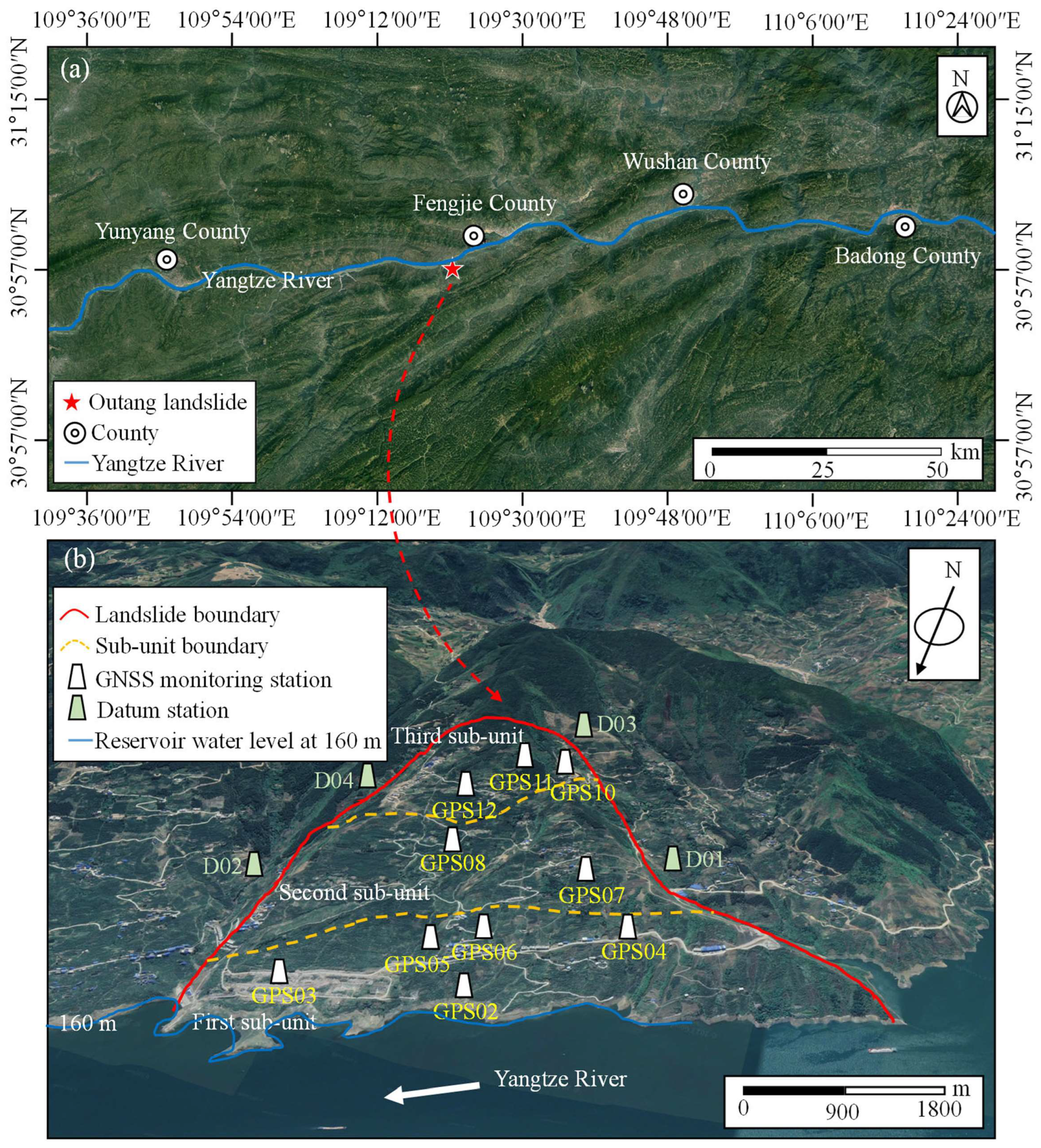
2.1. Geological Setting

The Outang landslide occurred in Fengjie County, Chongqing, China, which is situated on the south bank of the Yangtze River (Figure 1a). The landslide region experiences a subtropical monsoon climate. The annual precipitation in the landslide area averages 1147.9 mm, with the majority (around 70%) falling between May and September.

The landslide spans from 90 to 705 m, meaning that a portion of its toe is immersed in the reservoir water. The left boundary is defined by a ridge, while the right boundary is delineated by a gully. The slope varies from 5° to 50°, characterized by a steep upper section and a gentle lower section. The dimensions of the landslide range from 1640 to 2230 m in length and from 550 to 1300 m in width. The landslide exhibits an average thickness of 50.8 m, encompasses an area of 1.78 × 10⁶ m², and possesses a volume of 9 × 10⁷ m³. The landslide predominantly moves in the direction of 345°. Its sliding mass primarily consists of clayey soil, rock blocks, and fractured sandstone, with fractured sandstone being the predominant component. The bedrock comprises sandstone oriented at 335–350°/18–24°.

The landslide has been observed to experience three subunits of sliding. The first subunit extends from 90 to 370 m in elevation, with an area of 9.2 × 10⁵ m² and a volume of 6.48 × 10⁷ m³. Moving to the middle of the landslide, the second subunit encompasses an elevation range of 250 to 530 m, with an area of 3.2 × 10⁵ m² and a volume of 1.02 × 10⁷ m². The third subunit is at the top of the landslide, extending from 400 to 705 m, covering an area of 5.43 × 10⁴ m³ and having a volume of 1.45 × 10⁷ m³ [39].

2.2. Monitoring Scheme

Deformation of the Outang landslide has been observed since the Three Gorges Dam was impounded in 2003. To track the landslide’s movements, a monitoring system was implemented in 2006 and displacement monitoring data have been collected on a monthly basis since then. Following the update, twelve Global Navigation Satellite System (GNSS) monitoring points were installed on the Outang landslide in 2013 and provided three to six batches of displacement data every month. Since 6 August 2016, these monitoring points have been equipped with the capability to provide daily data, significantly enhancing the precision and frequency of measurements for monitoring the spatiotemporal movements of the Outang landslide. The automatic continuous GNSS monitoring stations exhibit precise measurements for surface displacement, with planimetry accuracy at 3 mm + 1 ppm and altimetry accuracy at 5 mm + 1 ppm. Utilizing a collection of single-frequency stations, the GNSS network transmits unprocessed data to the GNSS receiver at 20-second intervals. Subsequently, these raw data sets, which contain the relative positions of all measurement stations concerning datum stations, are collectively subjected to processing.

Furthermore, the twelve GNSS monitoring points, labeled as GPS01 to GPS 12, are strategically positioned within three distinct subunits. Monitoring stations GPS01 to GPS06 are situated in the first subunit, GPS07 to GPS09 are located in the second subunit, and GPS10 to GPS12 are positioned in the third subunit. Among these monitoring points, continuous displacement data are not available for GPS01 and GPS09. Four monitoring points, specifically labeled D01, D02, D03, and D04 have been installed outside the landslide area to serve as the datum stations (Figure 1b).

Real-time rainfall data from a weather station installed in Anping town, situated 3 km away from the Outang landslide, were adopted in this case. The daily reservoir water level data are accessible through a website (http://www.cjsyw.com, access on 1 September 2022) that is maintained by the Hydrology Bureau of Changjiang Water Resources Commission.

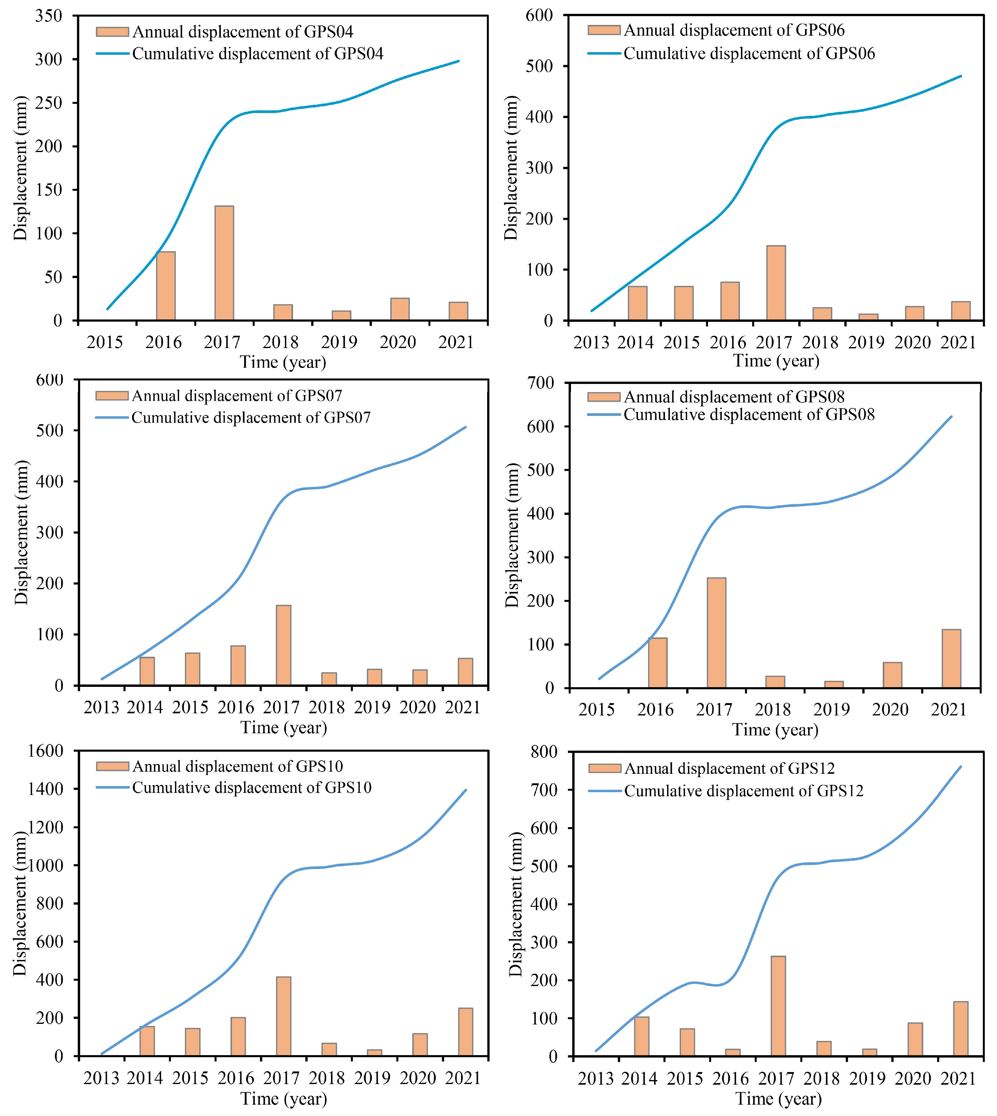
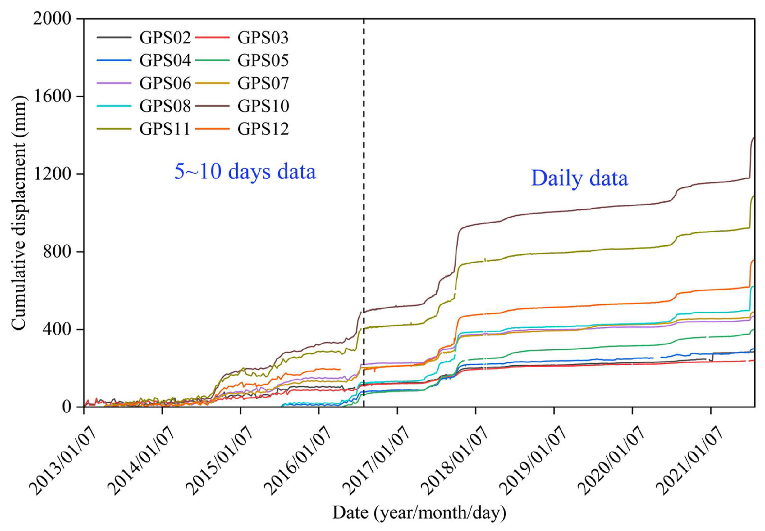
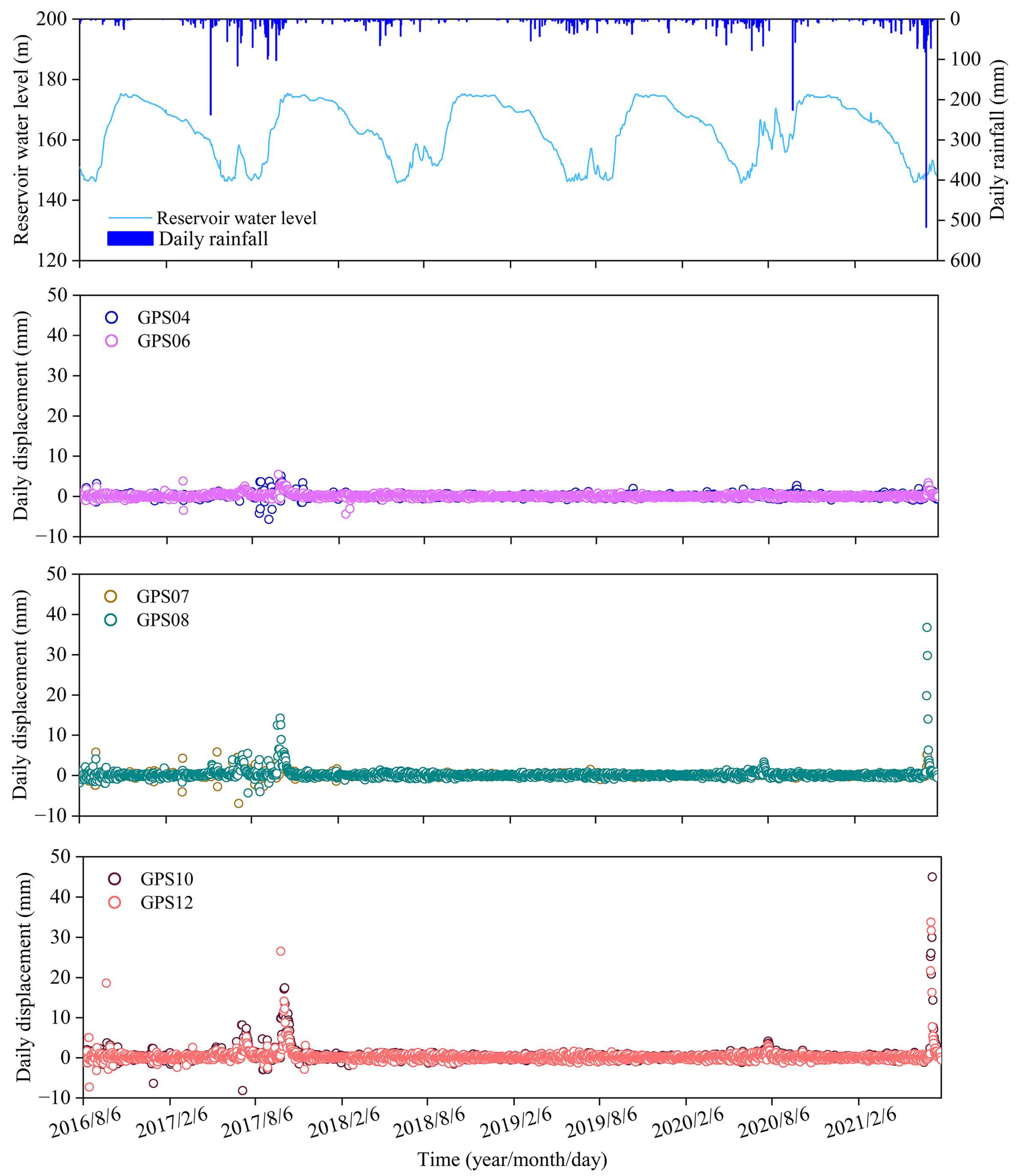
2.3. Monitoring Data

GNSS stations deliver monitored displacements across the slope. As of 31 July 2021, the cumulative displacements at the 10 monitoring stations decreased as follows (Figure 2): GPS10 > GPS11 > GPS12 > GPS08 > GPS07 > GPS06 > GPS05 > GPS02 > GPS04 > GPS03, indicating that the third subunit (GPS10 to GPS12) was the most active one in the three subunits with the second subunit being next (GPS07 and GPS08), and the first subunit suffered the smallest displacements (GPS03 to GPS06). Spatially, the displacement observations suggested that the deformation not only differs among the three subunits but also within the same subunit. Taking the third subunit as an example, the cumulative displacements of GPS10, GPS11, and GPS12 were 1393 mm, 1092, and 760 mm, respectively, displaying a decrease from the west to the east of the third subunit.

Six monitoring stations have been selected for further analysis, wherein GPS04 and GPS06 have been chosen as representative stations for the deformation of the first subunit. Similarly, GPS07 and GPS08 have been selected to represent the deformation of the second subunit, while GPS10 and GPS12 are designated as representative stations for the deformation of the third subunit (Figure 3). The six monitoring points were strategically selected to cover the three subunits of the landslide. Moreover, these monitoring stations provide extensive and complementary data for monitoring purposes. This configuration allows for a comprehensive assessment of the landslide behavior.

Annual displacement and cumulative displacement for the six GNSS stations are displayed in Figure 4. It should be noted that the displacement depicted in Figure 4 for 2021 only encompasses data up until July 31st, rather than the entire year. Over the course of the eight-year monitoring period, GPS10 registered the highest cumulative displacement, with an accumulation of 1.4 m. Additionally, it recorded an annual displacement of 425 mm in 2017 and a daily displacement of 17 mm on 6 October 2017.

Specifically, the annual displacement of GPS10 increased from 2013 and reached a peak in 2017 (425 mm). Subsequently, the annual displacements in 2018 and 2019 were significantly lower at 66 mm and 33 mm, respectively, representing only 15.5% and 7.8% of the displacement observed in 2017. In 2019, the landslide exhibited a significant resurgence in deformation, with a displacement measuring 116 mm. During the first seven months of 2021, the displacement reached 215 mm. The displacement observed at the remaining five monitoring stations (GPS04, GPS06, GPS07, GPS08, and GPS12) exhibited a similar trend to that of GPS10, characterized by a prominent deformation peak in 2017. Temporally, the deformation peak manifests periodically, with intervals of a few years, and consistently affects different parts of the landslide simultaneously.

3. Methodology

This study aims to propose a DL model for predicting landslide spatiotemporal displacement, employing techniques including the MIC, a CNN, LSTM, and an attention mechanism. The capacity of the MIC to capture both linear and nonlinear correlations between variables leads to quantitative evaluations of temporal hysteresis and spatial correlation. The CNN captures spatial correlation in landslide deformations, while LSTM excels in time series prediction. The integrated attention mechanism optimizes DL models. The rationale behind proposing an attention-based CNN-LSTM model for predicting landslide spatiotemporal displacement remains well founded. Additional details regarding the adopted techniques are elaborated upon in the Section 3.1 and Section 3.2. The procedure of the attention-based CNN-LSTM model is outlined in the Section 3.3. Accuracy indicators are displayed in Section 3.4.

3.1. Maximal Information Coefficient (MIC)

The Maximal Information Coefficient (MIC) is characterized by its generality and equitability, enabling it to capture both linear and nonlinear correlations between variable pairs [40]. Given n-pairs observations D = (P₁, P₂), where $P_1=\left\{p_1\left(i\right)\right\}$ and $P_2=\left\{p_2\left(i\right)\right\}$ with $i=1, 2, \cdots , n$, the MIC between P₁ and P₂ can be defined as follows:

(1)

P₁ and P₂ are partitioned into x rows or y columns by a division of x-by-y grids signed as G.

(2)

D|_G is calculated, which is the probability distribution of D on G. The maximum mutual information max I(D|_G) is achieved and then used to calculate the corresponding feature matrix $M{\left(D\right)}_{x,y}$ as follows.

$$\begin{array}{ll}M{\left(D\right)}_{x,y}=\frac{\max I\left({\mathrm{D}|}_G\right)}{\ln \min \left(x,y\right)}& \\ =\frac{\max \left({\sum }_{i=1}^x{\sum }_{i=1}^y\frac{n_{ij}}{N}ln\frac{n_{ij}}{N}-{\sum }_{i=1}^x\frac{{\sum }_{j=1}^y{n}_{ij}}{N}ln\frac{{\sum }_{j=1}^y{n}_{ij}}{N}-{\sum }_{i=1}^y\frac{{\sum }_{j=1}^x{n}_{ij}}{N}ln\frac{{\sum }_{j=1}^x{n}_{ij}}{N}\right)}{\ln \min \left(x,y\right)}& \end{array}$$

(1)

where n_ij is the number of samples in the cell of jth row and ith column and N is the amount of all samples.

(3)

A different G can lead to a different D|_G, and thus the globe optimal G₀ can be obtained by exhaustively searching the $M{\left(D\right)}_{x,y}$. The MIC between P₁ and P₂ is as follows.

$$MIC\left(D\right)=\underset{\mathit{xy}<B\left(\mathrm{N}\right)}{\max }\{{M\left(D\right)}_{x,y}=max\frac{\max I\left({\mathrm{D}|}_G\right)}{\ln \min \left(x,y\right)}={M\left(D\right)}_{x_0,y_0}$$

(2)

where B(N) is a function of the sample size and is commonly defined as N^0.6.

It has been proven that the MIC extends between 0 and 1, and the larger value donates the stronger correlation.

3.2. Deep Learning Approaches

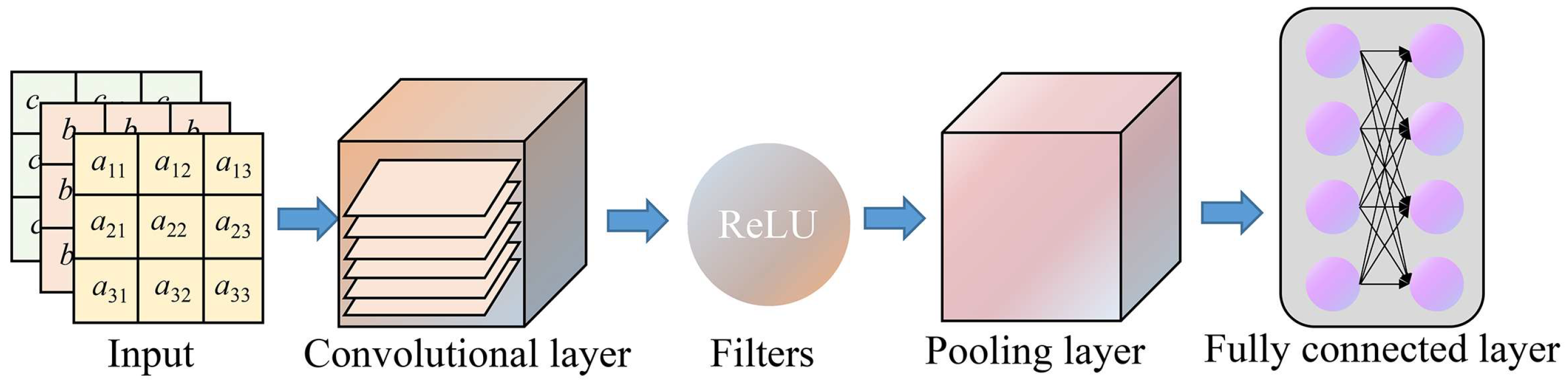
3.2.1. Convolutional Neural Network (CNN)

The convolutional neural network (CNN) represents a prominent deep learning framework, drawing inspiration from the innate visual perception mechanism found in living organisms [41]. Great state-of-the-art results on multiple domains have been achieved using CNN [42], including extracting the spatial structure relationship of multidimensional time series data [20]. Alongside the input and output layers, the CNN incorporates three additional types of layers, specifically the convolutional layers, pooling layers, and fully connected layers (Figure 5).

Convolutional layers utilize kernels as filters to generate feature maps by sliding across the given input date. This operation extracts spatial hierarchies of patterns and learns local feature representations, capturing important information. The resulting nonlinear outputs from the convolutional process are then passed through an activation function to adjust or truncate the generated output. The rectified linear unit (ReLU) presented as Equation (3), one of the most widely used nonlinearities in various fields, is employed in this study. The convolution operation is shown in Equation (4).

$$\mathrm{R}\mathrm{e}\mathrm{L}\mathrm{U}=\left\{\begin{array}{c}0, if x<0,\\ x, if \ge 0. \end{array}\right.$$

(3)

$$M_i=f(\sum M_{i-1}{⨂W}_i+b_i)$$

(4)

where $M_i$ is the input characteristic quantity of layer i; $f\left(x\right)$ is the activation function; $⨂$ is the convolution operation; and $W_i$ and $b_i$ are the weights and bias of kernel in layer i.

Pooling layers have a significant impact on reducing the spatial dimensions of the feature maps derived from convolutional layers. This process enhances the network’s ability to handle spatial variations and capture invariant features. Popular pooling operations include max pooling and average pooling. Among them, max pooling has demonstrated its effectiveness in numerous studies and is utilized in this study.

The fully connected layers connect all neurons obtained from the pooling process to every single neuron of the current layer, ultimately generating the final output. This configuration allows for comprehensive information integration and higher-level feature learning.

The initial values of some hyperparameters, such as the total number of features and size of features in the convolution process; the window size and window stride in the pooling process; and the number of neurons in a fully connected process, need to be set before training the model.

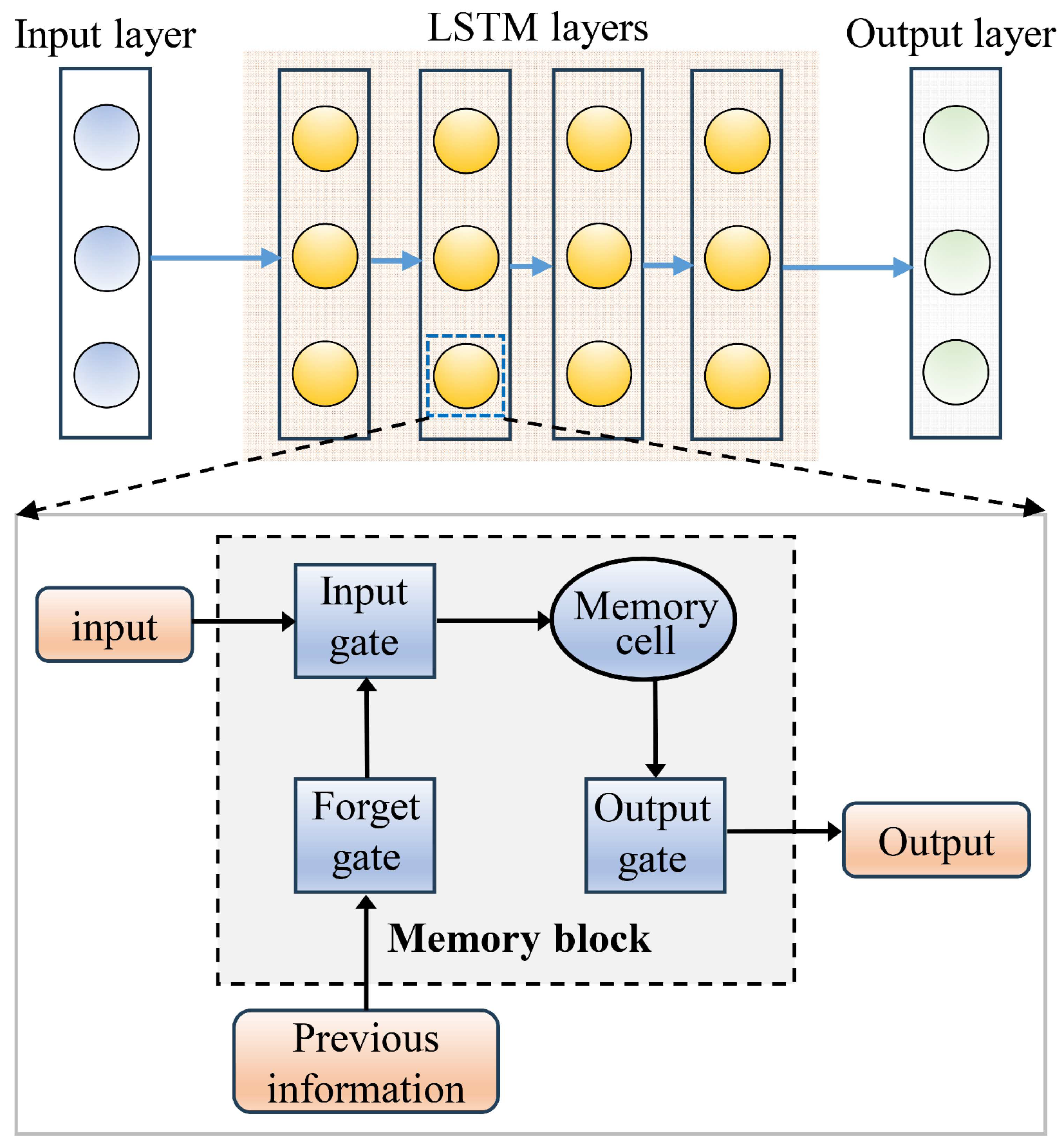
3.2.2. Long Short-Term Memory (LSTM) Neural Network

The long short-term memory (LSTM) neural network is an enhanced variant of the RNN, which overcomes issues like gradient explosion and vanishing gradients by incorporating “gates” into its architecture [43]. The fundamental component of the LSTM architecture is the memory block, which consists of an “input gate”, “forget gate”, “output gate”, and memory cell (Figure 6). These elements collectively facilitate valuable information while discarding irrelevant or redundant information over a long time series [44].

The principal algorithmic structure of LSTM is depicted by Equations (5)–(10). The input gate incorporates the input data into the memory cell by employing Equation (5). The forget gate, governed by Equation (6), controls the retention or dismissal of knowledge from the preceding time step. The output gate utilizes Equation (7) to regulate the transmission of output activations to other blocks.

$$i_t=\sigma (w_{xi}{x}_t+w_{hi}{h}_{t-1}+b_i)$$

(5)

$$f_t=\sigma \left(w_{xf}{x}_t+w_{hf}{h}_{t-1}+b_f\right)$$

(6)

$$o_t=\sigma (w_{xo}{x}_t+w_{ho}{h}_{t-1}+b_0)$$

(7)

$$g_t=\sigma \mathit{tanh}(w_{xc}{x}_t+w_{hc}{h}_{t-1}+b_c)$$

(8)

$$c_t=f_t{c}_{t-1}+i_t·g_t$$

(9)

$$h_t=o_t\mathit{tan}h(c_t)$$

(10)

where i_t, f_t, o_t, and c_t are the values of the input gate, forget gate, output gate, and memory cell in the memory block; b_i, b_f, b_o, and b_c are their corresponding bias values; $\sigma$ is the sigmoid function; and w_x and w_h are the input weights and hidden weights for the three gates.

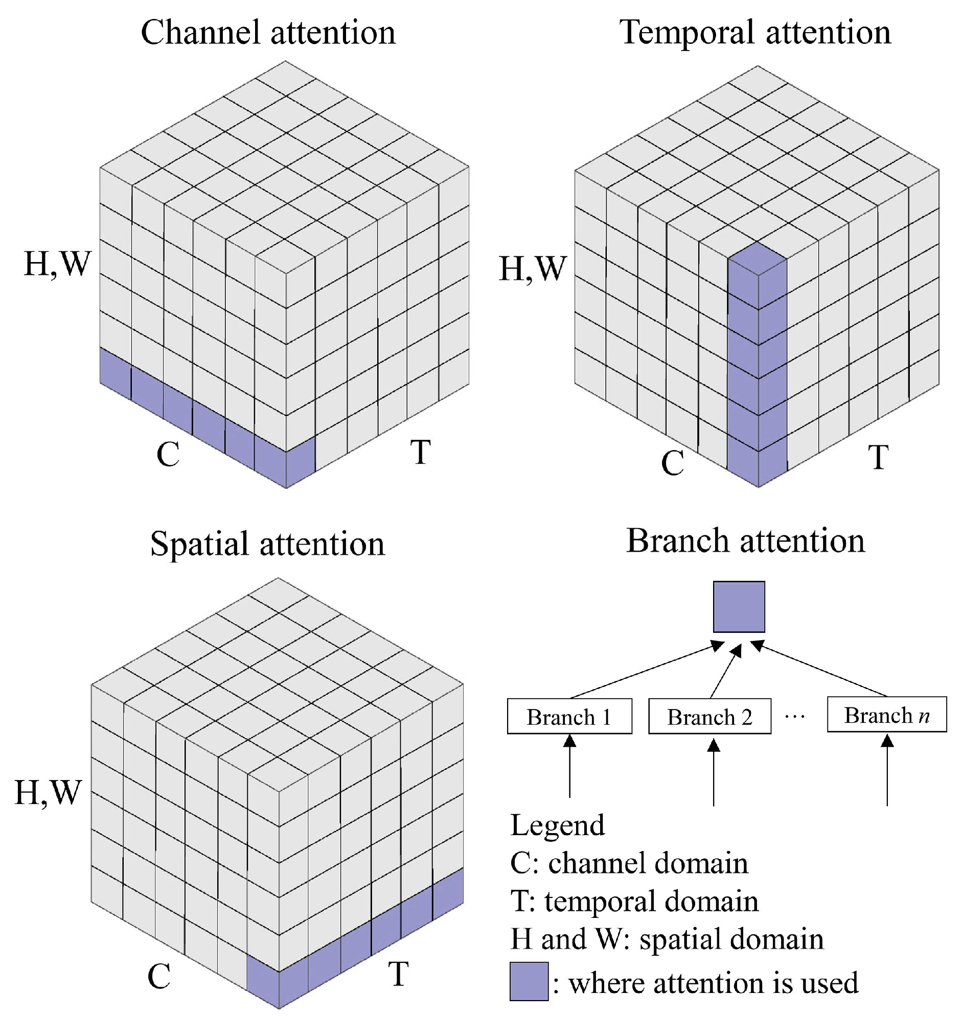
3.2.3. Attention Mechanism

The attention mechanism draws inspiration from the remarkable information processing abilities of humans, who possess the innate ability to selectively focus on distinctive elements within a sea of information [46,47]. In the realm of machine learning, attention manifests as a crucial component within models that autonomously learn and determine the significance of various parts of input data. Through adaptive weight adjustments that enhance significant information and suppress less relevant information, this mechanism facilitates model recalibration. Accordingly, the attention mechanism significantly enhances the optimization of conventional models [25,48].

Attention mechanisms mainly include channel attention, spatial attention, temporal attention, and branch attention [49]. Channel attention determines what elements to focus on, spatial attention determines where to allocate attention, temporal attention determines when to prioritize attention, and branch attention determines which elements to prioritize attention on (Figure 7).

In the context of spatiotemporal deformation prediction of landslides, the integration of spatial and temporal attention becomes crucial. Spatial and temporal attention jointly leverage the strengths of both types of attention, enabling the adaptive selection of significant regions and keyframes. Previous studies [50] have separately computed temporal and spatial attention, whereas some studies [51] have generated integrated spatiotemporal attention maps.

(1)

Spatial attention mechanism

Sequentially combining channel attention and spatial attention, the Convolutional Block Attention Module (CBAM) effectively utilizes both the spatial and cross-channel correlations of features to guide the network on what and where to emphasize [52]. The CBAM mechanism excels in highlighting pertinent channels and augmenting informative local regions. The lightweight architecture is particularly advantageous, as it seamlessly integrates into various CNN architectures with minimal additional computational overhead. This characteristic makes the CBAM an attractive choice for incorporating attention mechanisms into CNN models.

When provided with an input feature map $X\in R^{C\times H\times W}$, it performs a sequential calculation to compute a one-dimensional channel attention vector $s_c\in R^C$ and a two-dimensional spatial attention map $s_s\in R^{H\times W}$. To accomplish this, the CBAM employs two parallel branches that utilize max pooling and average pooling operations.

$$F_{avg}^c=A^s\left(X\right)$$

(11)

$$F_{max}^c=B^s\left(X\right)$$

(12)

$$s_c=\sigma (W_2\delta \left(W_1{F}_{avg}^c\right)+W_2\delta \left(W_1{F}_{max}^c\right))$$

(13)

$$M_C\left(X\right)=s_{c}X$$

(14)

where $A^s$ and $B^s$ denote global average pooling and global max pooling operations in the spatial domain, respectively. $\delta$ is ReLU activation. $\sigma$ is sigmoid activation. X is the input feature map.

The spatial attention employs a convolution layer with a large kernel to create the attention map:

$$F_{avg}^s=A^c\left(X\right)$$

(15)

$$F_{max}^s=B^c\left(X\right)$$

(16)

$$s_s=\sigma Conv\left[F_{avg}^s;F_{max}^s\right]$$

(17)

$$M_s\left(X\right)=s_{s}X$$

(18)

where $Conv(·)$ represents a convolution operation, while $A^c$ and $B^c$ are global pooling operations in the channel domain. The entire attention procedure is described as follows:

$$X^{\prime }=M_C\left(X\right)$$

(19)

$$Y=M_S\left(X^{\prime }\right)$$

(20)

(2)

Temporal attention mechanism

The inclusion of a temporal attention mechanism improves the adaptive acquisition of latent temporal dependency features within time series [53]. In the context of landslide displacement prediction, we utilize two separate LSTM networks. Initially, an attention mechanism is incorporated into one LSTM network to determine the weights of influencing factors at each time step. Subsequently, these weights are applied to the hidden state of each time step through the introduction of another temporal attention mechanism in the second LSTM network. This attention-based model effectively selects significant inputs based on their attention weights, capturing long-term temporal dependencies within time series. This enhancement greatly improves the prediction and generalization capabilities of LSTM networks.

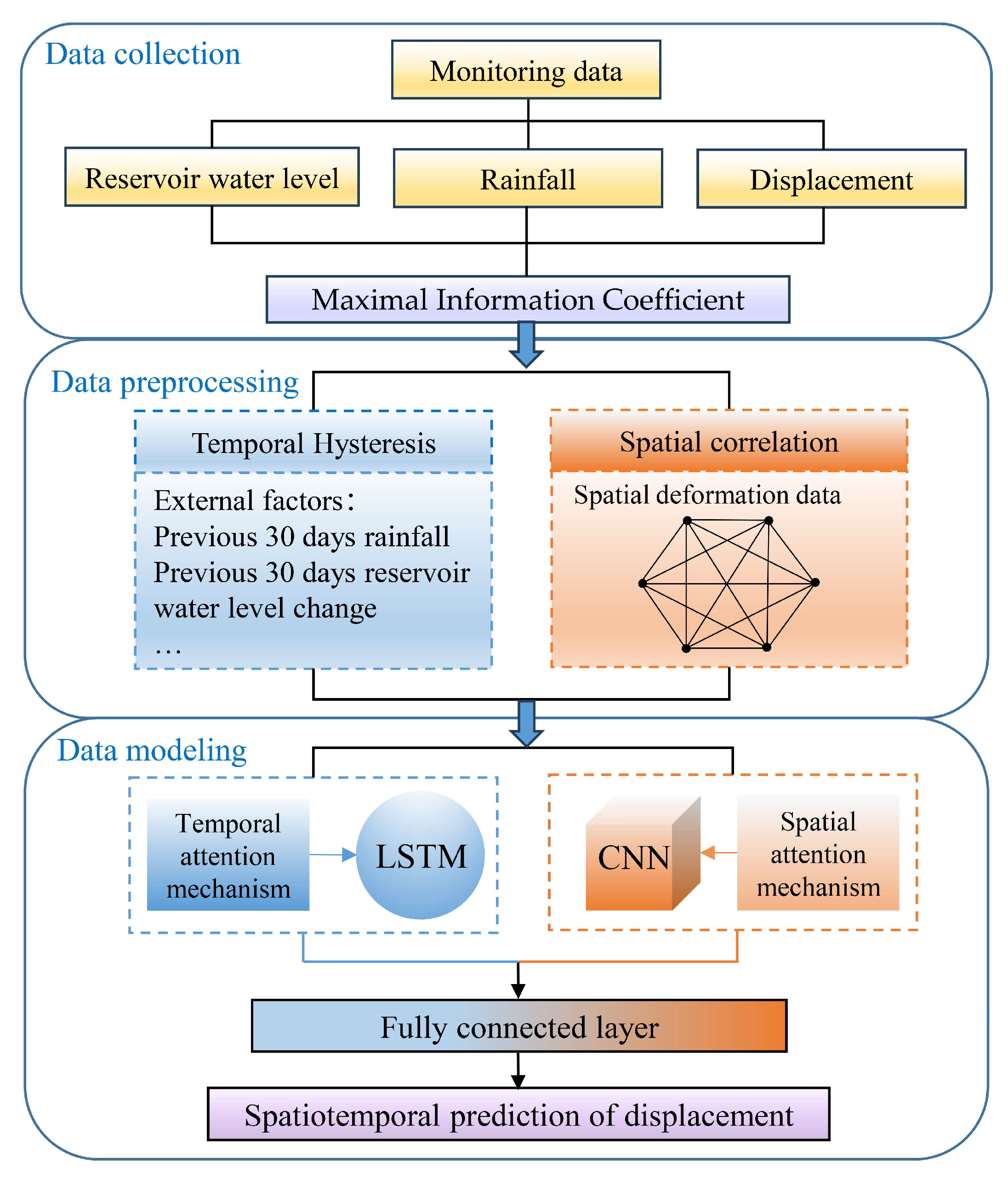
3.3. Workflow of Spatiotemporal Displacement Prediction

The spatiotemporal displacement prediction model comprises three components: data collection, data preprocessing, and data modeling. More specifically, the predictive modeling process is elaborated below, as shown in Figure 8.

(1)

Date collection

Multiple types of data have been meticulously collected from landslide monitoring systems, encompassing the reservoir water level, daily rainfall, and cumulative displacements. The comprehensive collection of these diverse data types forms the foundation for accurate and reliable predictions in the spatiotemporal displacement prediction model.

(2)

Data preprocessing

The MIC contributes to two key evaluations: (1) Quantifying the hysteresis between triggering factors and landslide displacement, thereby facilitating the selection of input data related to deformation-influencing factors for the forecasting model. (2) Assessing the correlation among displacements observed across various locations within the landslide region, thus substantiating the existence of spatial correlation. Furthermore, the spatial deformation data portray the deformation state of landslides, and consequently, it is also employed as a part of the input database for the proposed model.

(3)

Data modeling

The deformation forecasting model incorporates the CNN to extract spatial deformation correlations, and a spatial attention mechanism is implemented to optimize its performance. Simultaneously, the LSTM component captures the displacement time series. Temporal attention is integrated into the LSTM networks to further enhance their optimization. The combination of spatial correlation extraction through the CNN and time series analysis facilitated by LSTM enables the model to forecast landslide spatiotemporal displacement. This is accomplished by passing the fused information through a fully connected layer.

3.4. Evaluation of Model Accuracy

Four common measures, the root mean square error (RMSE), mean absolute percentage error (MAPE), absolute mean error (MAE), and coefficient of determination (R²), have been introduced for assessing the forecast accuracy of the proposed approach. Specifically, the RMSE is a measure that depends on the scale of the data. While the RMSE is valuable for the comparison among various approaches that apply to the same dataset, it is not suitable for comparing a single approach across datasets with varying scales. The MAPE is advantageous as it is independent of scale. Therefore, it is commonly employed to assess forecast performance across diverse datasets. Nevertheless, a drawback of the MAPE is that it becomes infinite or undefined when the observation is zero [22]. The MAE assesses the mean of the overall prediction error and its changes exhibit linearity, thereby making it intuitively comprehensible. The R² quantifies the model’s degree of fit, providing a measure of the alignment between the predicted and observed data [54]. Lower RMSE, MAPE, and MAE values, along with a higher R², indicate a superior prediction performance. The detailed mathematical expressions are as follows:

$$RMSE=\sqrt{\frac{1}{N}\sum _{i=1}^N{\left(x_i-{\widehat{x}}_i\right)}^2}$$

(21)

$$MAPE=\frac{1}{N}\sum _{i=1}^N\left|\frac{x_i-{\widehat{x}}_i}{x_i}\right|\times 100\%$$

(22)

$$R^2=1-\frac{{\sum }_{i=1}^N{\left(x_i-{\widehat{x}}_i\right)}^2}{{\sum }_{i=1}^N{\left(x_i-\overline{x}\right)}^2}$$

(23)

$$MAE=\frac{1}{N}\sum _{i=1}^N\left({{\widehat{x}}_i - x}_i\right)$$

(24)

where $x_i$ represents the observation; ${\widehat{x}}_i$ represents the prediction; $\overline{x}$ represents the average value of the observations; and N represents the number of measurements.

The nonparametric Friedman test is employed to identify significant differences among multiple forecasting models from four performance measures (RMSE, MAPE, MAE, and R²) [55,56]. This test proceeds as outlined below:

(1)

Execute forecasting models to predict the displacements of landslides and gather the values of performance measures as datasets. In this study, the predicted outcomes from each chosen monitoring station serve as individual datasets.

(2)

The m, n, and k denote the number of forecasting models, datasets, and performance measures, respectively. For the ith indicator, the forecasting models are ranked from 1 to m, represented as $r_i^j$.

(3)

For the jth forecasting model, the average rank can be determined.

$$R_j=\frac{1}{n}\sum _i^j{r}_i^j$$

(25)

(4)

The Friedman statistic, denoted as F_f, can be calculated.

$$F_f=\frac{12n}{m(m+1)}\left(\sum R_j^2 - \frac{m{(m+1)}^2}{4}\right)$$

(26)

A p-value is used to determine the probability of rejecting the null hypothesis. If a p-value is less than 0.05, the null hypothesis should be dismissed, highlighting a statistically significant variation among the forecasting models [57].

4. Result

4.1. Spatiotemporal Correlation of Landslide Displacement

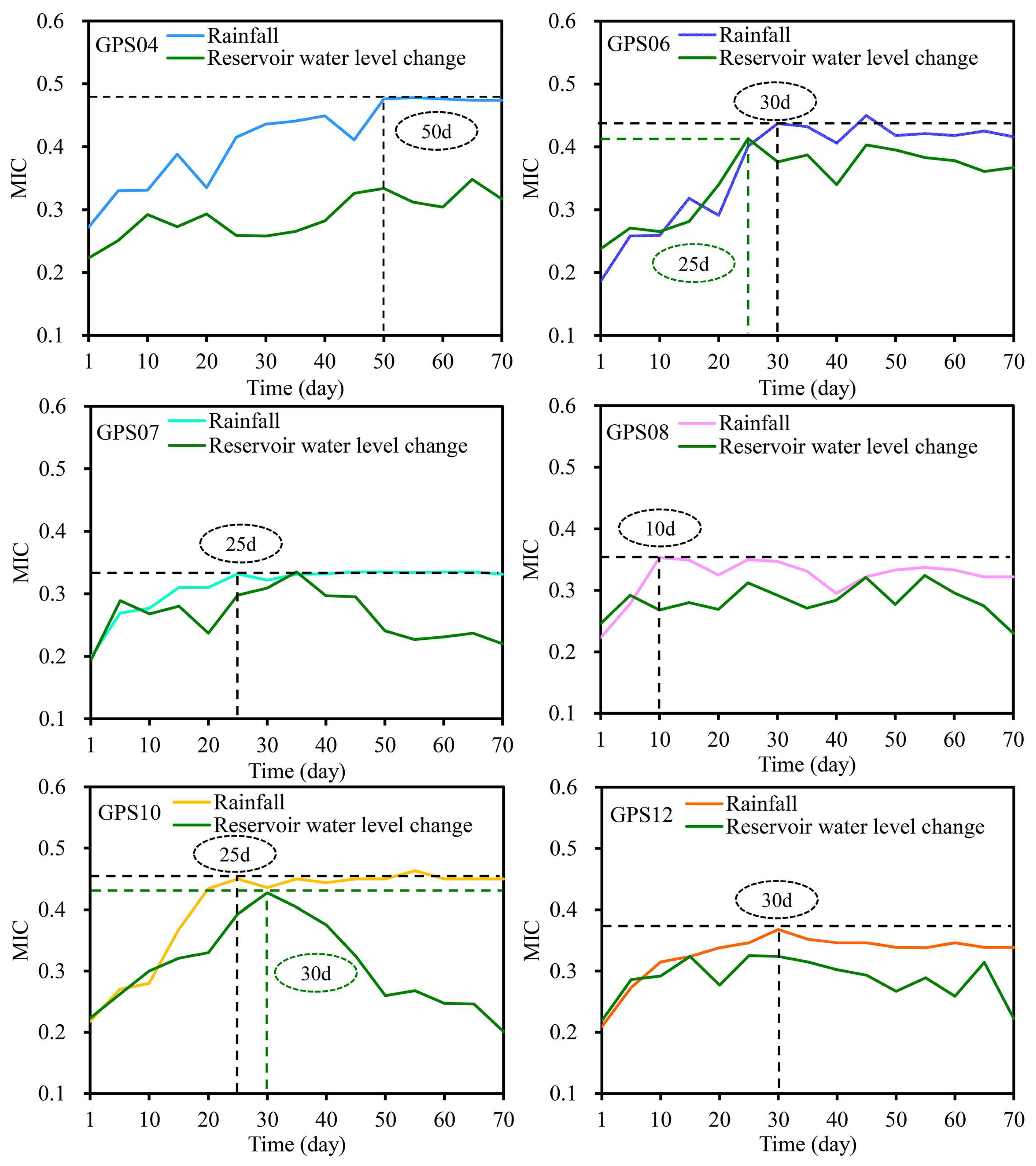
4.1.1. Temporal Correlation between Landslide Displacement and External Factors

Reservoir water level changes and rainfall usually cannot induce landslide deformation immediately. Their hysteresis effect on landslide deformation has been considered by Yang et al. [33]. In addition, as analyzed in Section 2.3, the deformation characteristics of the landslide vary spatially. We selected six monitoring points (GPS04, GPS06, GPS07, GPS08, GPS10, and GPS12) that span across the entirety of the landslide area. Through the utilization of the MIC method, we conducted a quantitative analysis to examine the correlation and hysteresis effects of rainfall and reservoir level changes on daily displacements. The program for the MIC was implemented using Python 3.6 within the Anaconda 3 environment. Figure 9 provides a comprehensive summary of the MIC values, which were obtained by evaluating the correlation between the daily displacement rate and cumulative rainfall as well as the changes in reservoir water level over a time range of 1 to 70 days.

According to Figure 9, it was evident that the MIC values between daily displacement and either the daily rainfall or daily reservoir level change were notably lower. This observation suggested the existence of a hysteresis effect caused by these two triggering factors on landslide deformation. The MIC values obtained from the six GNSS stations exhibited a discernible pattern of initially increasing and then reaching a stable state as the cumulative rainfall from previous days increased. We designated the point at which this trend shifted as the turning point, representing the lag time between the effect of rainfall and the subsequent landslide deformation. This turning point was highlighted by black ellipses in Figure 9. From the perspective of the response time to rainfall, GPS08 was the most sensitive location, and the response time was 10 days. Conversely, GPS04 needed 50 days of cumulative rainfall to trigger locational deformation. For the other four monitoring points, GPS06, GPS07, GPS10, and GPS12, the response time was 25 to 30 days.

The MIC values of the reservoir water level change were found to be lower compared to those for rainfall. This observation can be attributed to the fact that the six monitoring points were not situated in close proximity to the reservoir water. The response time to the reservoir water level change for GPS06 and GPS10 was 30 days. Nevertheless, as shown in the MIC curves of the reservoir water level change for GPS04, GPS07, GPS08, and GPS12, no peak points were observed, which indicated that the lag time for the two locations was not identified.

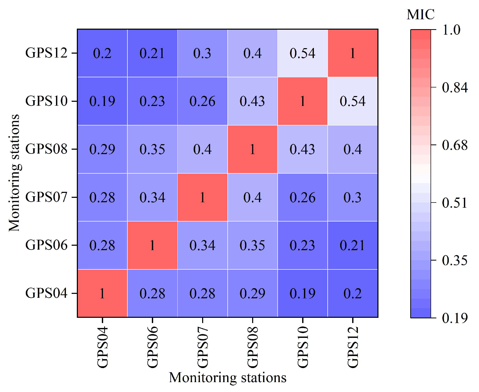
4.1.2. Spatial Correlation between Various Locations of the Outang Landslide

The MIC was also utilized to assess the correlation of deformation between different spatial parts of the landslide by analyzing the displacements of GPS04, GPS06, GPS07, GPS08, GPS10, and GPS12. Notably, daily displacements before August 6th, 2016, were not available, and the data between 7 August 2016 and 31 July 2021 were adopted in the analysis of spatial correlation. The results of the MIC are shown in Figure 10.

Significant correlations were identified between the movement of GPS08 and monitoring points in the first subunit (GPS04 and GPS06), as well as GPS07 in the second subunit. In terms of the correlation analysis, GPS08 and GPS12, positioned within the second and third subunits, respectively, exhibited the highest MIC values with the displacement of GPS10. It was worth noting that the displacement of GPS10 stood out as the largest among all the monitored points. In brief, the local movement can be most influenced by the deformation occurring in nearby locations with the largest displacement. However, it is crucial to acknowledge that this influence is confined within a specific scope of the landslide. According to the MIC results among the six stations, it is noteworthy that the highest MIC values for GPS04, GPS06, and GPS07 are associated with GPS08 rather than GPS10, despite GPS10 experiencing the most significant deformation.

4.2. Spatiotemporal Displacement Prediction of the Outang Landslide Using Attention-Based CNN-LSTM

Displacement prediction is a crucial and ongoing topic in the field of landslide studies. It enables us to gain insights into how landslides respond to various influencing factors and provides valuable information about future stability. According to analysis of temporal hysteresis and spatial correlation for GNSS displacement, it can be inferred that displacement prediction involves not only the displacement time series but also the spatial impact from other stations. The spatiotemporal prediction of landslide displacement is undertaken using the attention-based CNN-LSTM model.

4.2.1. Procedure of Attention-Based CNN-LSTM Model

A feature matrix, denoted as $X_s$, is created based on the deformation data collected from monitoring points covering the landslide. Each element in $X_s$ represents a deformation station within the monitoring system. For the Outang landslide, a total of six monitoring points (GPS04, GPS06, GPS07, GPS08, GPS10, and GPS12) are selected, which are distributed across two longitudinal profiles and three subunits of the landslide. Consequently, a feature matrix with dimensions of two rows and three columns is employed to store the deformation information spanning the landslide. This matrix is considered to capture the spatial deformation features of the landslide. In each element of the feature matrix $X_s$, three indicators are recorded and considered as the input data of the CNN: the cumulative displacement, displacement rate, and acceleration.

Moreover, in the context of utilizing the LSTM model for time series forecasting, the input data consists of the reservoir water level and the 30-day change in the reservoir water level, as well as the cumulative rainfall over the preceding 30 days. These specific features are incorporated into the model based on their relevance and significance (Section 4.1), and their selection aligns with the existing literature [22,58,59].

Daily monitoring data spanning from 6 August 2016 to 30 June 2021 are selected as the training dataset. Subsequently, the period from 1 July 2021, to 31 July 2021, is designated as the prediction sample to evaluate the performance of the model. All the data, including the displacement of each monitoring point and external triggers, are normalized to [−1, 1].

The proposed model is implemented using Python 3.6 within the Anaconda 3 environment, leveraging PyTorch 1.9.0 as the backend [60]. The Adaptive Moment Estimation Optimizer (Adam), an optimization algorithm in PyTorch, is used for updating model parameters during neural network training [61]. The specifications pertinent to the workstation utilized for the experimental procedures are delineated in

Table 1. Specifications of the workstation.

Specifications	Details
CPU	Intel i7-1165G7
Operating System	Windows10
GPU Memory	16 GB
GPU	MX350
Development Language	Python 3.6
Development Environment	Anaconda 3
Machine Learning Framework	PyTorch 1.9.0

. The CNN algorithm comprises one convolutional layer with a kernel size of (4, 4). The LSTM algorithm adopts a single LSTM layer with a hidden size of 64. The training process involves 100 iterations to optimize the performance and convergence.

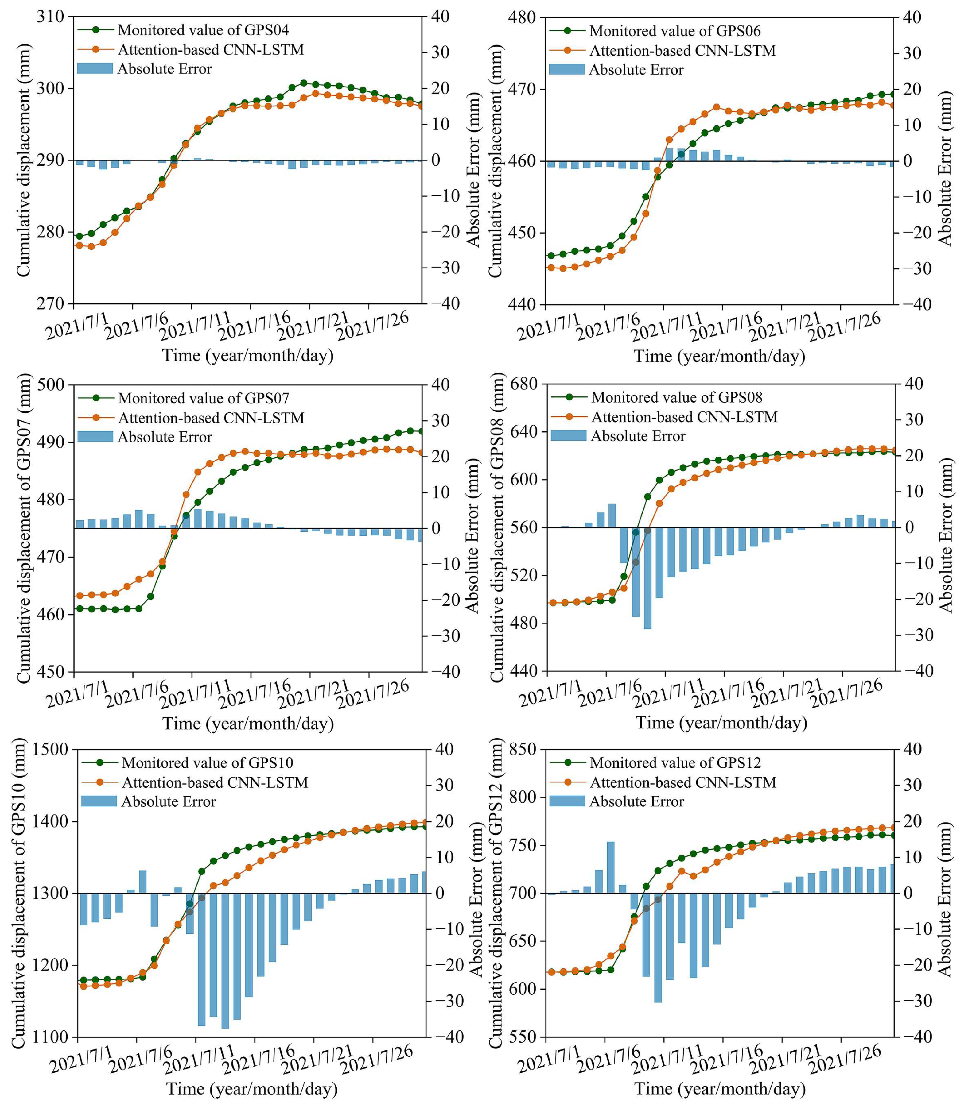
4.2.2. Prediction Results of Attention-Based CNN-LSTM Model

The predicted displacement results of the six monitoring stations are presented in

Table 2. Displacement prediction accuracy of GPS04, GPS06, GPS07, GPS08, GPS10, and GPS12 using attention-based CNN-LSTM model.

Accuracy	GPS04	GPS06	GPS07	GPS08	GPS10	GPS12
RMSE (mm)	1.18	1.80	2.84	9.64	16.21	11.91
MAE (mm)	0.99	1.51	2.47	6.29	10.95	8.58
MAPE (%)	0.34	0.33	0.52	1.07	0.82	1.18
R2	0.9752	0.9555	0.9444	0.9989	0.9654	0.9580

and Figure 11. It appears that the predicted displacement aligns closely with the monitored values, indicating a good fit. The RMSE values exhibited a range spanning from 1.18 to 16.21 mm, with the MAE values ranging from 0.99 to 10.95 mm. Notably, the minimum and maximum values for these two evaluation indices were observed in the cases of GPS04 and GPS10, respectively. The MAPE values ranged from 0.33% (GPS06) to 1.18% (GPS12) across the six monitoring stations. The R² values for all the six stations exceeded 0.94, and the GPS08 station was particularly noteworthy with a value of 0.9989.

The cumulative displacements of GPS04, GPS06, and GPS07 were found to be smaller compared to GPS08, GPS10, and GPS12. The maximum absolute errors recorded for GPS04, GPS06, and GPS07 were 2.94 mm, 3.39 mm, and 5.27 mm, respectively, while GPS08, GPS10, and GPS12 exhibited values of 36.78 mm, 44.98 mm, and 33.78 mm, respectively (Figure 11). Further analysis was conducted on the forecasting accuracy of the attention-based CNN-LSTM model for monitoring stations GPS08, GPS10, and GPS12.

As depicted in Figure 11, from 1 July 2021 to 7 July 2023, the cumulative displacements of these three stations remained nearly constant, with the displacement rates being 0. The forecasting model demonstrated a satisfactory performance, with absolute errors consistently below 10 mm. During the period from 8 July 2021 to 12 July 2023, the landslide experienced severe deformation. The average displacement rates recorded for GPS08, GPS10, and GPS12 were 21.35 mm, 29.41 mm, and 22.24 mm, respectively. Significant errors were observed during this period, with the largest absolute error in daily displacement prediction for the three stations being approximately 30 mm. From 13 July 2023 to 31 July 2023, the landslide once again stabilized, with average displacement rates below 5 mm for the three monitoring stations. Moreover, there was a gradual decrease in absolute error. It was evident that the attention-based CNN-LSTM model effectively captured the deformation trend and demonstrated a satisfactory prediction performance during this period of steady deformation.

4.2.3. Accuracy Comparison of the LSTM Model, CNN-LSTM Model, and Attention-Based CNN-LSTM Model

To facilitate a more comprehensive comparison of the spatiotemporal prediction model with an attention mechanism, namely the attention-based CNN-LSTM, we established two additional models: a single monitoring point LSTM model and a spatiotemporal prediction CNN-LSTM model without an attention mechanism. The comparison of predicted and measured values from these three models (LSTM model, CNN-LSTM model, and attention-based CNN-LSTM model) on six monitoring stations (GPS04, GPS06, GPS07, GPS08, GPS10, and GPS12) is illustrated in Figure 12. Throughout the timeframe spanning from 1 July 2021 to 31 July 2021, the models demonstrated higher prediction accuracy during the steady deformation phase within the landslide. However, their prediction performance decreased relatively during periods of significant displacement increase.

The RMSE, MAE, MAPE, and R² from the three forecasting models on the six monitoring stations are displayed in Figure 13:

(1)

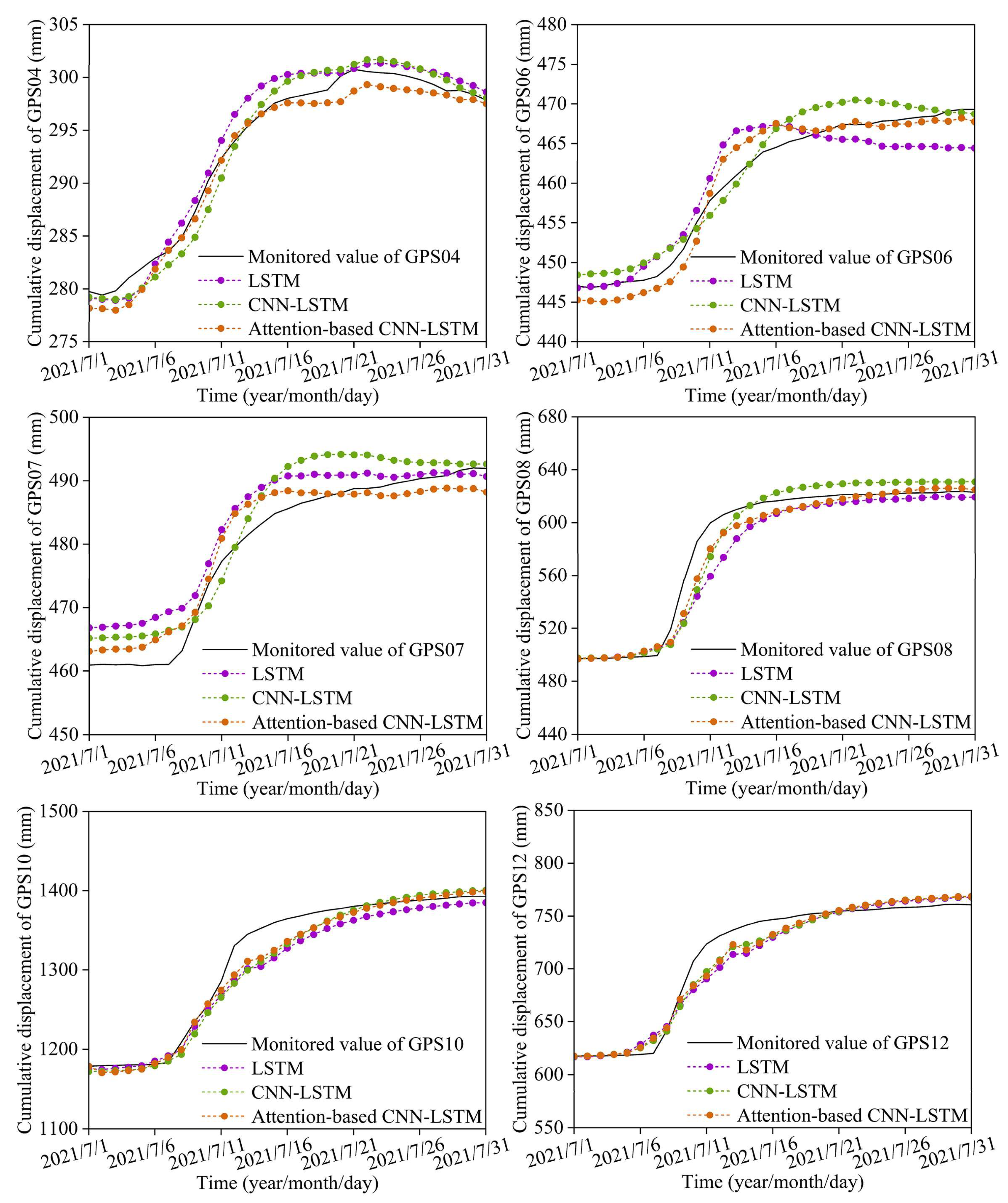
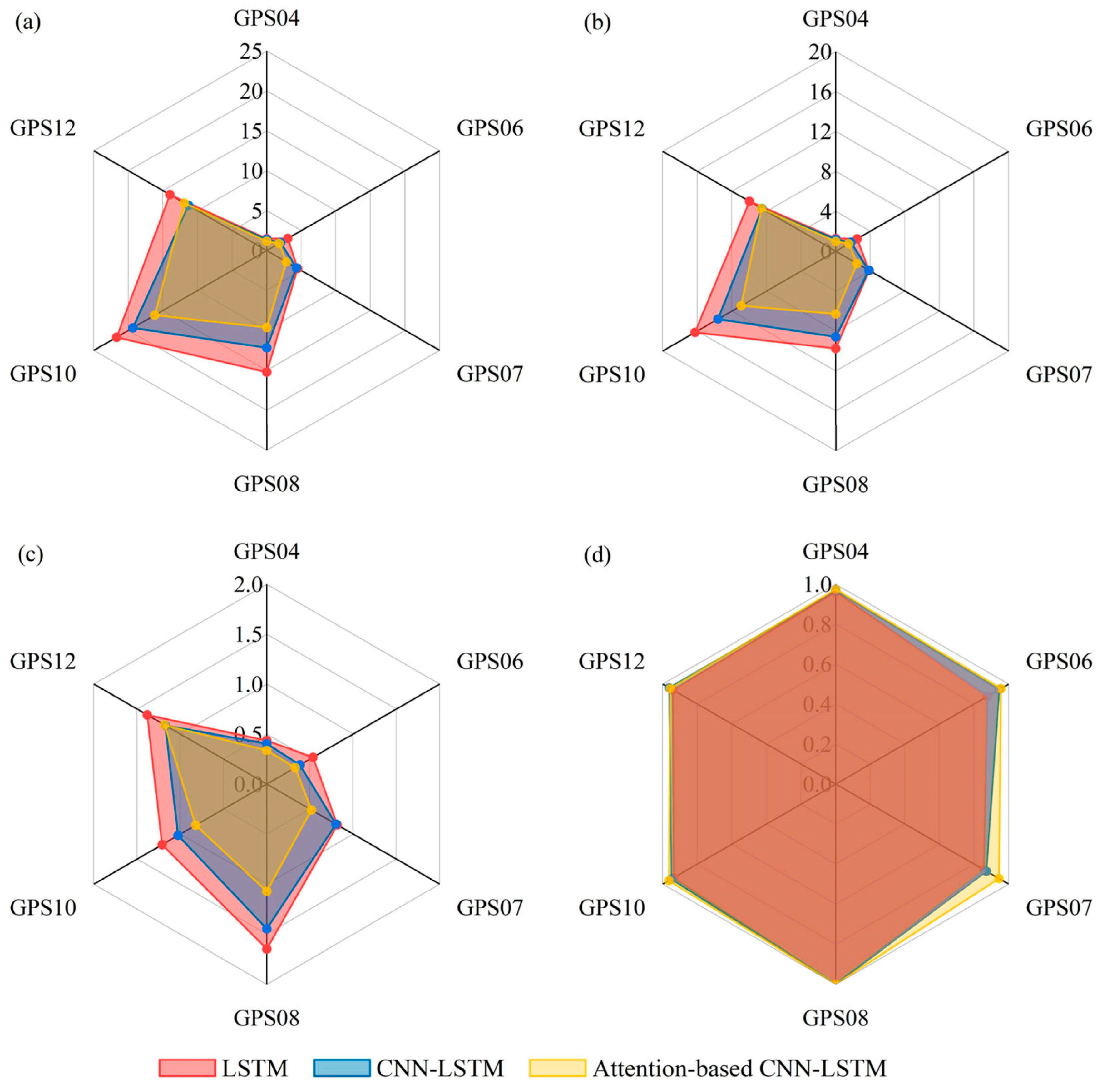
According to Figure 13a,b, the attention-based CNN-LSTM model exhibited a smaller RMSE and MAE than both the LSTM model and CNN-LSTM model, indicating a superior prediction performance, particularly for GPS08 and GPS10. However, it was important to note that the attention-based CNN-LSTM model did not consistently outperform the other models on GPS04, GPS06, GPS07, and GPS12. The forecasting accuracy of the proposed model was even worse than the CNN-LSTM model for GPS12.

(2)

Derived from Figure 13c, the attention-based CNN-LSTM model exhibited varying prediction performances across the six GPS monitoring stations. Notably, for GPS04, which had a relatively smaller displacement rate, the forecasting model demonstrated a better prediction performance compared to stations with larger displacement rates, such as GPS08, GPS10, and GPS12. This pattern was also observed in the LSTM model and CNN-LSTM model.

(3)

The R² values of the attention-based CNN-LSTM model consistently surpassed those of the other two models across all six monitoring points, signifying an enhanced capability in predicting the observed behavior (Figure 13d). Within the attention-based CNN-LSTM model, R² values for these stations ranged from 0.9444 (GPS07) to 0.9989 (GPS08). In comparison, the R² ranges were wider for the CNN-LSTM model (0.8715 for GPS07 to 0.9982 for GPS01) and the LSTM model (0.8573 for GPS07 to 0.9973 for GPS08). This suggested that the LSTM model can achieve a commendable prediction performance for specific individual points, yet it lacked consistency across all monitoring points within the landslide due to its inability to account for spatial correlation. While both models take spatial correlation into consideration, the attention-based CNN-LSTM model exhibited a superior prediction performance compared to the CNN-LSTM model. This enhancement can be attributed to the incorporation of a spatial–temporal attention mechanism, which optimizes the performance of the DL model.

(4)

The nonparametric Friedman test was employed to discern significant differences among the models used. In this research, we worked with three forecasting models (m), evaluated them across four performance measures (n), and used six distinct datasets (k). The procedure was executed using the SPSS software (IBM SPSS Statistics 27.0.1, Chicago, IL, USA). The p-values of the RMSE, MAPE, MAE, and R² were all less than 0.05, suggesting a statistically significant variation among the LSTM, CNN-LSTM, and attention-based CNN-LSTM models.

5. Discussion

5.1. Spatiotemporal Deformation Analysis of the Outang Landslide

The Outang landslide exhibited both temporal and spatial variations in deformation behavior. Over the course of the eight-year monitoring period from 2016 to 2021, significant deformation was observed in 2017, whereas the landslide remained relatively stable in the other years. Additionally, the reservoir water level experienced periodic fluctuations ranging from 145 to 175 m. In 2017, the annual rainfall reached a substantial amount of 1636 mm, greatly exceeding the multiyear average rainfall of 1147.9 mm. It can be inferred that the strong deformation can be induced by abundant rainfall.

However, it should be noted that heavy rainfall does not necessarily guarantee the occurrence of severe deformation in different parts of the landslide. This phenomenon is clearly observed in the case of monitoring stations GPS04 and GPS06, belonging to the first subunit. These stations recorded a maximum daily displacement of approximately 5 mm. In contrast, the second subunit, represented by GPS07 and GPS8, exhibited a maximum daily displacement of 15 mm, while the third subunit, represented by GPS10 and GPS12, displayed a significantly higher maximum value of 30 mm (Figure 3).

These variations in displacement highlight the complex nature of the landslide response to rainfall and suggest that other factors may also be at play in determining the extent of deformation. Besides the difference in local inherent conditions across various sections of the landslide and the interaction of deformation between the subunits, another factor that can contribute to the deformation variability is the response of each subunit to external factors. The quantitative analysis conducted in Section 4.1 to examine the temporal correlation between landslide displacement and external factors serves as potential evidence. The findings from this analysis provide potential evidence that both rainfall and reservoir activities have a hysteresis effect on landslide deformation. Moreover, it was observed that the lag time between these external factors and the corresponding deformation varied across different parts of the landslide.

Furthermore, we conducted a quantitative analysis to examine the spatial correlation among the displacements of GNSS stations across the overall landslide area. Our analysis revealed that the movement of one location within this landslide can be impacted by other nearby areas, particularly those adjacent locations experiencing significant deformation. This spatial interplay contributes to the complex deformation characteristics observed within the landslide, adding an additional layer of intricacy to the overall behavior of the landslide. Therefore, the incorporation of this spatial interplay is crucial when conducting deformation analysis, predicting displacements, and performing other associated tasks within landslide early warning systems [25].

5.2. Applications, Limitation, and Potential of the Attention-Based CNN-LSTM Model for Spatiotemporal Displacement Prediction

The attention-based CNN-LSTM model employs a combination of a CNN to capture the spatial correlation among deformation points and LSTM to catch the temporal dependencies in the time series in the proposed forecasting model. Additionally, the attention mechanism autonomously learns and determines the significance of various parts of input data, which significantly enhances the optimization of the CNN-LSTM model. The deformation of specific locations within the Outang landslide can be significantly influenced by the nearby movement, a phenomenon that has been substantiated and elaborated upon in “Section 4.1.2 Spatial correlation between various locations of the Outang Landslide”. Therefore, it is reasonable to incorporate spatial correlation into the spatiotemporal displacement prediction.

One remarkable improvement offered by the attention-based CNN-LSTM model is its capacity to simultaneously forecast multiple monitoring points. This enhanced capability enables the model to manage multiple predictions more efficiently, aligning with findings from previous studies. Consequently, the proposed model holds the potential to be applicable to early warnings of landslide scenarios worldwide that share similar characteristics. The proposed model exhibits remarkable prediction performance when applied to the six monitoring stations of the Outang landslide. Conversely, certain spatiotemporal displacement prediction models demonstrate inconsistent accuracy across different monitoring points within a single landslide [25,26]. The Outang landslide boasts over 1800 data points, whereas other cases in these studies typically contain 300 or fewer. Besides the inherent differences in the models, the quantity and quality of the data from landslide cases could be another contributing factor. Additionally, Xi et al. [25] observed that although the GCN-LSTM and GCN-GRU models displayed similar prediction accuracies, the GCN-LSTM took approximately 1.6 times longer than the GCN-GRU. One should, in the future, enhance the running efficiency of models while ensuring the prediction accuracy will be improved in the future.

Six monitoring stations were chosen for spatiotemporal displacement prediction instead of utilizing all the GNSS stations. The absence of comprehensive monitoring data in certain stations makes their inclusion impractical. Furthermore, the rationale behind the station selection is closely tied to the specific data prerequisites of the CNN employed within this framework. Specifically, the CNN is employed to extract the spatial correlation of deformations, which requires the input data to possess strict Euclidean spatial characteristics. This means the distances between data points can be measured using straight-line or Euclidean distance while maintaining the properties of Euclidean space. Satisfying this requirement can be challenging as the placement of monitoring points is typically based on the specific deformation locations of landslides.

6. Conclusions

The surficial movements of the Outang landslide have been extensively documented over a span of eight years using GPS data, with nearly five years of daily data available. The recent daily monitored data of landslide movement confirms the presence of both temporal and spatial variations in deformation within the Outang landslide. A quantitative study using the MIC was conducted to analyze the spatial correlation among different locations of the Outang landslide and the temporal correlation between landslide displacement and external triggers. Considering external influencing factors and spatial correlation within the Outang landslide, an attention-based CNN-LSTM model is proposed to predict the spatiotemporal displacement. The conclusions are as follows:

Monitoring points located at different locations exhibit varying response times to external factors. GPS08 and GPS04 are the two monitoring stations that exhibit the highest and lowest responsiveness, respectively, in terms of rainfall, with lagging time intervals of 10 days and 50 days. The remaining four GNSS monitoring stations have lag times ranging from 25 to 30 days. Additionally, the MIC results reveal that there is mutual influence among different locations within the landslide, especially in the case of nearby sites experiencing significant deformation. This influence has a more pronounced impact on the surrounding areas. GPS10, in particular, serves as one such monitoring station for the Outang landslide. The quantitative analysis conducted on the deformation triggers of landslides and the spatial correlation, utilizing daily monitoring data and the MIC method, provides valuable insights for predicting displacements and carrying out other associated tasks within landslide early warning systems.

The attention-based CNN-LSTM model was utilized to forecast spatiotemporal displacement on the Outang landslide. This model incorporates a CNN for spatial correlation, LSTM for capturing temporal dependencies, and a spatial–temporal attention mechanism to enhance optimization. In comparison to the LSTM model and CNN-LSTM model, the attention-based CNN-LSTM model demonstrates a superior prediction performance, especially when applied to monitoring stations with larger displacement rates. By accurately predicting the severe deformation of landslides, the attention-based CNN-LSTM model can significantly enhance the efficacy of early warning systems, enabling timely interventions to mitigate the risks associated with landslides.

It should be noted that the forecasting accuracy of the attention-based CNN-LSTM model varies across multiple monitoring stations within a landslide, with better predictions observed for locations experiencing steady deformation compared to those with severe deformation. However, particular attention should be given to the prediction of severe deformation parts, as accurate predictions in these areas are of the utmost importance.

References

1. Guzzetti, F.; Gariano, S.; Peruccacci, S.; Marchesiniet, B.I.; Rossi, M.; Melillo, M. Landslide early warning systems. Earth Sci. Rev. 2020, 200, 102973. [Google Scholar] [CrossRef]
2. Wang, Y.; Wen, H.J.; Sun, D.; Li, Y.C. Quantitative assessment of landslide risk based on susceptibility mapping using random forest and GeoDetector. Remote Sens. 2021, 13, 2625. [Google Scholar] [CrossRef]
3. Bravo-López, E.; Fernández, D.C.T.; Sellers, C.; Delgado-García, J. Landslide susceptibility mapping of landslides with Artificial Neural Networks: Multi-approach analysis of Backpropagation Algorithm applying the neuralnet package in Cuenca, Ecuador. Remote Sens. 2022, 14, 3495. [Google Scholar] [CrossRef]
4. Miao, F.S.; Zhao, F.C.; Wu, Y.P.; Li, L.W.; Török, Á. Landslide susceptibility mapping in Three Gorges Reservoir Area based on GIS and Boosting Decision Tree model. Stoch. Environ. Res. Risk Assess. 2023, 37, 2283–2303. [Google Scholar] [CrossRef]
5. Wen, H.J.; Xiao, J.F.; Xiang, X.K.; Wang, X.F.; Zhang, W.G. Singular spectrum analysis-based hybrid PSO-GSA-SVR model for predicting displacement of step-like landslides: A case of Jiuxianping landslide. Acta Geotech. 2023, 1–18. [Google Scholar] [CrossRef]
6. Park, J.Y.; Lee, S.R.; Lee, D.H.; Kim, Y.T.; Lee, J.S. A regional-scale landslide early warning methodology applying statistical and physically based approaches in sequence. Eng. Geol. 2019, 260, 105193. [Google Scholar] [CrossRef]
7. Pecoraro, G.; Calvello, M.; Piciullo, L. Monitoring strategies for local landslide early warning systems. Landslides 2019, 16, 213–231. [Google Scholar] [CrossRef]
8. Yin, Y.P.; Wang, H.D.; Gao, Y.L.; Li, X.C. Real-time monitoring and early warning of landslides at relocated Wushan Town, the Three Gorges Reservoir, China. Landslides 2010, 7, 339–349. [Google Scholar] [CrossRef]
9. Macciotta, R.; Hendry, M.; Martin, C.D. Developing an early warning system for a very slow landslide based on displacement monitoring. Nat. Hazards 2020, 81, 887–907. [Google Scholar] [CrossRef]
10. Lacroix, P.; Handwerger, A.L.; Bievre, G. Life and death of slow moving landslides. Nat. Rev. Earth Environ. 2020, 1, 404–419. [Google Scholar] [CrossRef]
11. Shihabudheen, K.V.; Pillai, G.N.; Peethambaran, B. Prediction of landslide displacement with controlling factors using extreme learning adaptive neuro-fuzzy inference system (ELANFIS). Appl. Soft Comput. 2017, 61, 892–904. [Google Scholar] [CrossRef]
12. Yao, W.M.; Li, C.D.; Guo, Y.C.; Criss, E.R.; Zuo, Q.J.; Zhan, H.B. Short-term deformation characteristics, displacement prediction, and kinematic mechanism of Baijiabao landslide based on updated monitoring data. Bull. Eng. Geol. Environ. 2022, 81, 393. [Google Scholar] [CrossRef]
13. Tehrani, F.S.; Calvello, M.; Liu, Z.Q.; Zhang, L.M.; Suzanne, L. Machine learning and landslide studies: Recent advances and applications. Nat. Hazards 2022, 114, 1197–1245. [Google Scholar] [CrossRef]
14. Liu, Y.; Xu, C.; Huang, B.; Ren, X.W.; Liu, C.Q.; Hu, B.D.; Chen, Z. Landslide displacement prediction based on multi-source data fusion and sensitivity state. Eng. Geol. 2020, 271, 105608. [Google Scholar] [CrossRef]
15. Shihabudheen, K.; Peethambaran, B. Landslide displacement prediction technique using improved neuro-fuzzy system. Arab. J. Geosci. 2017, 10, 502. [Google Scholar] [CrossRef]
16. Catani, F. Landslide detection by deep learning of non-nadiral and crowdsourced optical images. Landslides 2021, 18, 1025–1044. [Google Scholar] [CrossRef]
17. Huang, F.M.; Zhang, J.; Zhou, C.B.; Wang, Y.H.; Huang, J.S.; Zhu, L. A deep learning algorithm using a fully connected sparse autoencoder neural network for landslide susceptibility prediction. Landslides 2020, 17, 217–229. [Google Scholar] [CrossRef]
18. Guo, Z.Z.; Tian, B.; Li, G.; Huang, D.; Zeng, T.; He, J.; Song, D. Landslide susceptibility mapping in the Loess Plateau of northwest China using three data-driven techniques-a case study from middle Yellow River catchment. Front. Earth Sci. 2023, 10, 1033085. [Google Scholar] [CrossRef]
19. Prakash, E.; Manconi, A.; Loew, S. Mapping landslides on EO data: Performance of deep learning models vs. traditional machine learning models. Remote Sens. 2020, 12, 346. [Google Scholar] [CrossRef]
20. Li, L.M.; Wang, C.Y.; Wen, Z.Z.; Gao, J.; Xia, M.F. Landslide displacement prediction based on the ICEEMDAN, ApEn and the CNN-LSTM models. J. Mt. Sci. 2023, 20, 1220–1231. [Google Scholar] [CrossRef]
21. Wang, L.Q.; Ting, X.; Liu, S.L.; Zhang, W.G.; Yang, B.B.; Chen, L.C. Quantification of model uncertainty and variability for landslide displacement prediction based on Monte Carlo simulation. Gondwana Res. 2023, 123, 27–40. [Google Scholar] [CrossRef]
22. Yang, B.B.; Yin, K.L.; Lacasse, S.; Liu, Z.Q. Time series analysis and long short-term memory neural network to predict landslide displacement. Landslides 2019, 16, 677–694. [Google Scholar] [CrossRef]
23. Yang, B.B.; Xiao, T.; Wang, L.Q.; Huang, W. Using complementary ensemble empirical mode decomposition and gated recurrent unit to predict landslide displacements in dam reservoir. Sensors 2022, 22, 1320. [Google Scholar] [CrossRef]
24. Nava, L.; Carraro, E.; Reyes, C.C.; Puliero, S.; Bhuyan, K.; Rosi, A.; Monserrat, O.; Floris, M.; Meena, S.R.; Galve, J.P.; et al. Landslide displacement forecasting using deep learning and monitoring data across selected sites. Landslides 2023, 20, 2111–2129. [Google Scholar] [CrossRef]
25. Xi, N.; Zang, M.D.; Lin, R.S.; Sun, Y.J.; Mei, G. Spatiotemporal prediction of landslide displacement using deep learning ap-proaches based on monitored time-series displacement data: A case in the Huanglianshu landslide. Georisk 2023, 17, 98–113. [Google Scholar] [CrossRef]
26. Jiang, Y.N.; Luo, H.Y.; Xu, Q.; Lu, Z.; Liao, L.; Li, H.J.; Hao, L.N. A graph convolutional incorporating GRU network for landslide displacement forecasting based on spatiotemporal analysis of GNSS observations. Remote Sens. 2022, 14, 1016. [Google Scholar] [CrossRef]
27. Khalili, M.A.; Guerriero, L.; Pouralizadeh, M.; Calcaterra, D.; Martire, D.D. Monitoring and prediction of landslide-related deformation based on the GCN-LSTM algorithm and SAR imagery. Nat. Hazards 2023, 119, 39–68. [Google Scholar] [CrossRef]
28. Guzzetti, F.; Peruccacci, S.; Rossi, M.; Stark, C.P. Rainfall thresholds for the initiation of landslides in central and southern Europe. Meteorol. Atmos. Phys. 2007, 98, 239–267. [Google Scholar] [CrossRef]
29. Medina, V.; Hürlimann, M.; Guo, Z.Z.; Lloret, A.; Vaunat, J. Fast physically-based model for rainfall-induced landslide susceptibility assessment at regional scale. Catena 2021, 201, 105213. [Google Scholar] [CrossRef]
30. Guo, Z.Z.; Torra, O.; Hürlimann, M.; Abancó, C.; Medina, V. FSLAM: A QGIS plugin for fast regional susceptibility assessment of rainfall-induced landslides. Environ. Model. Softw. 2022, 150, 105354. [Google Scholar] [CrossRef]
31. Hürlimann, M.; Guo, Z.Z.; Puig-Polo, C.; Medina, V. Impacts of future climate and land cover changes on landslide suscepti-bility: Regional scale modeling in the Val d’Aran region (Pyrenees, Spain). Landslides 2022, 19, 99–118. [Google Scholar] [CrossRef]
32. Agterberg, F. How Can Earth Science Help Reduce the Adverse Effects of Climate Change? J. Earth Sci. 2022, 33, 1338. [Google Scholar] [CrossRef]
33. Yang, H.Q.; Song, K.L.; Chen, L.C.; Qu, L.L. Hysteresis effect and seasonal step-like creep deformation of the Jiuxianping landslide in the Three Gorges Reservoir region. Eng. Geol. 2023, 317, 107089. [Google Scholar] [CrossRef]
34. Yao, W.M.; Li, C.D.; Zuo, Q.J.; Zhan, H.B.; Criss, R.E. Spatiotemporal deformation characteristics and triggering factors of Baijiabao landslide in Three Gorges Reservoir region, China. Geomorphology 2019, 343, 34–47. [Google Scholar] [CrossRef]
35. Wu, Q.; Tang, H.M.; Ma, X.H.; Wu, Y.P.; Hu, X.L.; Wang, L.Q.; Criss, R.; Yuan, Y.; Xu, Y.J. Identification of movement charac-teristics and causal factors of the Shuping landslide based on monitored displacements. Bull. Eng. Geol. Environ. 2019, 78, 2093–2106. [Google Scholar] [CrossRef]
36. Jiang, P.; Chen, J.J. Displacement prediction of landslide based on generalized regression neural networks with K-fold cross-validation. Neurocomputing 2016, 198, 40–47. [Google Scholar] [CrossRef]
37. Song, K.; Wang, F.W.; Yi, Q.L.; Lu, S.Q. Landslide deformation behavior influenced by water level fluctuations of the Three Gorges Reservoir (China). Eng. Geol. 2018, 247, 58–68. [Google Scholar] [CrossRef]
38. Wang, H.; Long, G.Y.; Shao, P.; Lv, Y.; Gan, F.; Liao, J.X. A DES-BDNN based probabilistic forecasting approach for step-like landslide displacement. J. Clean. Prod. 2023, 394, 136281. [Google Scholar] [CrossRef]
39. Guo, Z.Z.; Chen, L.X.; Gui, L.; Du, J.; Yin, K.L.; Do, H.M. Landslide displacement prediction based on variational mode de-composition and WA-GWO-BP model. Landslides 2020, 17, 567–583. [Google Scholar] [CrossRef]
40. Reshef, D.N.; Reshef, Y.; Mitzenmacher, M.; Sabeti, P. Equitability analysis of the Maximal Information Coefficient with comparisons. Comput. Sci. 2013, preprint. [Google Scholar] [CrossRef]
41. Gu, J.X.; Wang, Z.H.; Kuen, J.; Ma, L.Y.; Shahroudy, A.; Shuai, B.; Liu, T.; Wang, X.X.; Wang, G.; Cai, J.F.; et al. Recent advances in convolutional neural networks. Pattern Recognit. 2018, 77, 354–377. [Google Scholar] [CrossRef]
42. Nagi, J.; Ducatelle, F.; Caro, G.A.D.; Cireşan, D.; Meier, U.; Giusti, A.; Nagi, F.; Schmidhuber, J.; Gambardella, L.M. Max-pooling convolutional neural networks for vision-based hand gesture recognition. In Proceedings of the IEEE International Conference on Signal and Image Processing Applications (ICSIPA), Kuala Lumpur, Malaysia, 16–18 November 2011; pp. 342–347. [Google Scholar] [CrossRef]
43. Hochreiter, S.; Schmidhuber, J. Long short-term memory. Neural Comput. 1997, 9, 1735–1780. [Google Scholar] [CrossRef]
44. Felix, A.F.; Jürgen, S. Recurrent nets that time and count. In Proceedings of the IEEE-INNS-ENNS International Joint Conference on Neural Network, Como, Italy, 27 July 2000; Volume 3, pp. 189–194. [Google Scholar] [CrossRef]
45. Liu, Z.Q.; Guo, D.; Suzanne, L.; Li, J.H.; Yang, B.B.; Choi, J.C. Algorithms for intelligent prediction of landslide displacements. Zhejiang Univ. Sci. A 2020, 21, 412–429. [Google Scholar] [CrossRef]
46. Rensink, R.A. The dynamic representation of scenes. Vis. Cogn. 2002, 7, 17–42. [Google Scholar] [CrossRef]
47. Corbetta, M.; Shulman, G.L. Control of goal-directed and stimulus-driven attention in the brain. Nat. Rev. Neurosci. 2002, 3, 201–215. [Google Scholar] [CrossRef]
48. Ren, Q.B.; Li, M.C.; Li, H.; Shen, Y. A novel deep learning prediction model for concrete dam displacements using interpretable mixed attention mechanism. Adv. Eng. Inf. 2021, 50, 101407. [Google Scholar] [CrossRef]
49. Guo, M.H.; Xu, T.X.; Liu, J.J.; Liu, Z.N.; Jiang, P.T.; Mu, T.J.; Zhang, S.H.; Martin, R.R.; Cheng, M.M.; Hu, S.M. Attention mechanisms in computer vision: A survey. Vis. Media 2022, 8, 331–368. [Google Scholar] [CrossRef]
50. Song, S.; Lan, C.; Xing, J.; Zeng, W.; Liu, J. An endto-end spatio-temporal attention model for human action recognition from skeleton data. In Proceedings of the 31st AAAI Conference on Artificial Intelligence, San Francisco, CA, USA, 4–9 February 2017; pp. 4263–4270. [Google Scholar] [CrossRef]
51. Fu, Y.; Wang, X.Y.; Wei, Y.C.; Huang, T. STA: Spatial-temporal attention for large-scale video-based person re-identification. In Proceedings of the AAAI Conference on Artificial Intelligence, Honolulu, HI, USA, 29–31 January 2019; Volume 33, pp. 8287–8294. [Google Scholar] [CrossRef]
52. Woo, S.; Park, J.; Lee, J.; Kweon, I.S. CBAM: Convolutional block attention module. In Proceedings of the European Conference on Computer Vision (ECCV), Munich, Germany, 8–14 September 2018; pp. 3–19. [Google Scholar] [CrossRef]
53. Liu, Y.Q.; Zhang, Q.; Song, L.H.; Chen, Y.Y. Attention-based recurrent neural networks for accurate short-term and long-term dissolved oxygen prediction. Comput. Electron. Agric. 2019, 165, 104964. [Google Scholar] [CrossRef]
54. Saurabh, K.; Sunil, F.R. Context aware recommendation systems: A review of the state of the art techniques. Comput. Sci. Rev. 2020, 37, 100255. [Google Scholar] [CrossRef]
55. Ma, J.W.; Xia, D.; Wang, Y.K.; Niu, X.X.; Jiang, S.; Liu, Z.Y.; Guo, H.X. A comprehensive comparison among metaheuristics (MHs) for geohazard modeling using machine learning: Insights from a case study of landslide displacement prediction. Eng. Appl. Artif. Intell. 2022, 114, 105150. [Google Scholar] [CrossRef]
56. Ma, J.W.; Xia, D.; Guo, H.X.; Wang, Y.K.; Niu, X.X.; Liu, Z.Y.; Jiang, S. Metaheuristic-based support vector regression for landslide displacement prediction: A comparative study. Landslides 2022, 19, 2489–2511. [Google Scholar] [CrossRef]
57. Demšar, J. Statistical comparisons of classifiers over multiple data sets. J. Mach. Learn. Res. 2006, 7, 1–30. [Google Scholar]
58. Wang, L.; Wu, C.; Yang, Z.Y.; Wang, L.Q. Deep learning methods for time-dependent reliability analysis of reservoir slopes in spatially variable soils. Comput. Geotech. 2023, 159, 105413. [Google Scholar] [CrossRef]
59. Guo, Z.Z.; Chen, L.X.; Yin, K.L.; Shrestha, D.P.; Zhang, L. Quantitative risk assessment of slow-moving landslides from the viewpoint of decision-making: A case study of the Three Gorges Reservoir in China. Eng. Geol. 2020, 273, 105667. [Google Scholar] [CrossRef]
60. Ketkar, N.; Moolayil, J. Introduction to PyTorch. In Deep Learning with Python; Apress: Berkeley, CA, USA, 2020; pp. 27–91. [Google Scholar] [CrossRef]
61. Kingma, D.P.; Ba, J. Adam: A method for stochastic optimization. In Proceedings of the 3rd International Conference on Learning Representations, San Diego, CA, USA, 7–9 May 2015. [Google Scholar] [CrossRef]
Figure 1. (a) Location of the Outang landslide; (b) arrangement of GNSS monitoring stations.
Remotesensing 15 04971 g001
Figure 2. Cumulative displacements of GNSS monitoring stations on Outang landslide between 1 July 2013 and 31 July 2021.
Remotesensing 15 04971 g002
Figure 3. Daily displacements of GPS monitoring stations on Outang landslide between 6 August 2016 and 31 July 2021.
Remotesensing 15 04971 g003
Figure 4. Annual and cumulative displacement of GPS04, GPS06, GPS07, GPS08, GPS10, and GPS12.
Remotesensing 15 04971 g004
Figure 5. Convolutional neural network (CNN) architecture.
Remotesensing 15 04971 g005
Figure 6. Long short-term memory (LTSM) neural network architecture [22,45].
Remotesensing 15 04971 g006
Figure 7. Schematic of four primary categories of attention mechanism [49].
Remotesensing 15 04971 g007
Figure 8. Procedure of attention-based CNN-LSTM model.
Remotesensing 15 04971 g008
Figure 9. The MIC between daily displacement rate and various days’ cumulative rainfall/reservoir water level change.
Remotesensing 15 04971 g009
Figure 10. Correlation between the displacements of GPS04, GPS06, GPS07, GPS08, GPS10, and GPS12.
Remotesensing 15 04971 g010
Figure 11. Comparison of predicted and measured displacement at monitoring locations of GPS04, GPS06, GPS07, GPS08, GPS10, and GPS12.
Remotesensing 15 04971 g011
Figure 12. Comparison between attention-based CNN-LSTM, CNN-LSTM, and LSTM.
Remotesensing 15 04971 g012
Figure 13. Quantitative evaluation visualization results for different forecasting models: (a) RMSE; (b) MAE; (c) MAPE; and (d) R2.
Remotesensing 15 04971 g013