Abstract
This article presents a method to detect and segment mine waste deposits, specifically waste rock dumps and leaching wasted dumps, in Sentinel-2 satellite imagery using artificial intelligence. This challenging task has important implications for mining companies and regulators like the National Geology and Mining Service in Chile. Challenges include limited knowledge of mine waste deposit numbers, as well as logistical and technical difficulties in conducting inspections and surveying physical stability parameters. The proposed method combines YOLOv7 object detection with a vision transformer classifier to locate mine waste deposits, as well as a deep generative model for data augmentation to enhance detection and segmentation accuracy. The ViT classifier achieved 98% accuracy in differentiating five satellite imagery scene types, while the YOLOv7 model achieved an average precision of 81% for detection and 79% for segmentation of mine waste deposits. Finally, the model was used to calculate mine waste deposit areas, with an absolute error of 6.6% compared to Google Earth API results.
1. Introduction
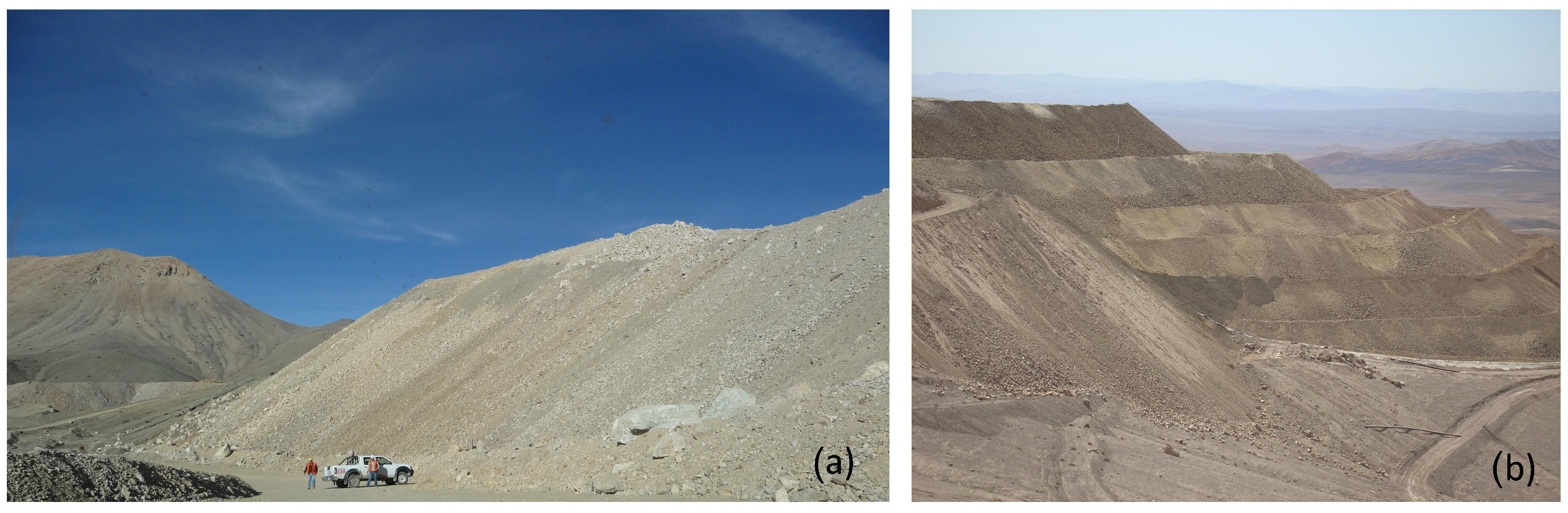
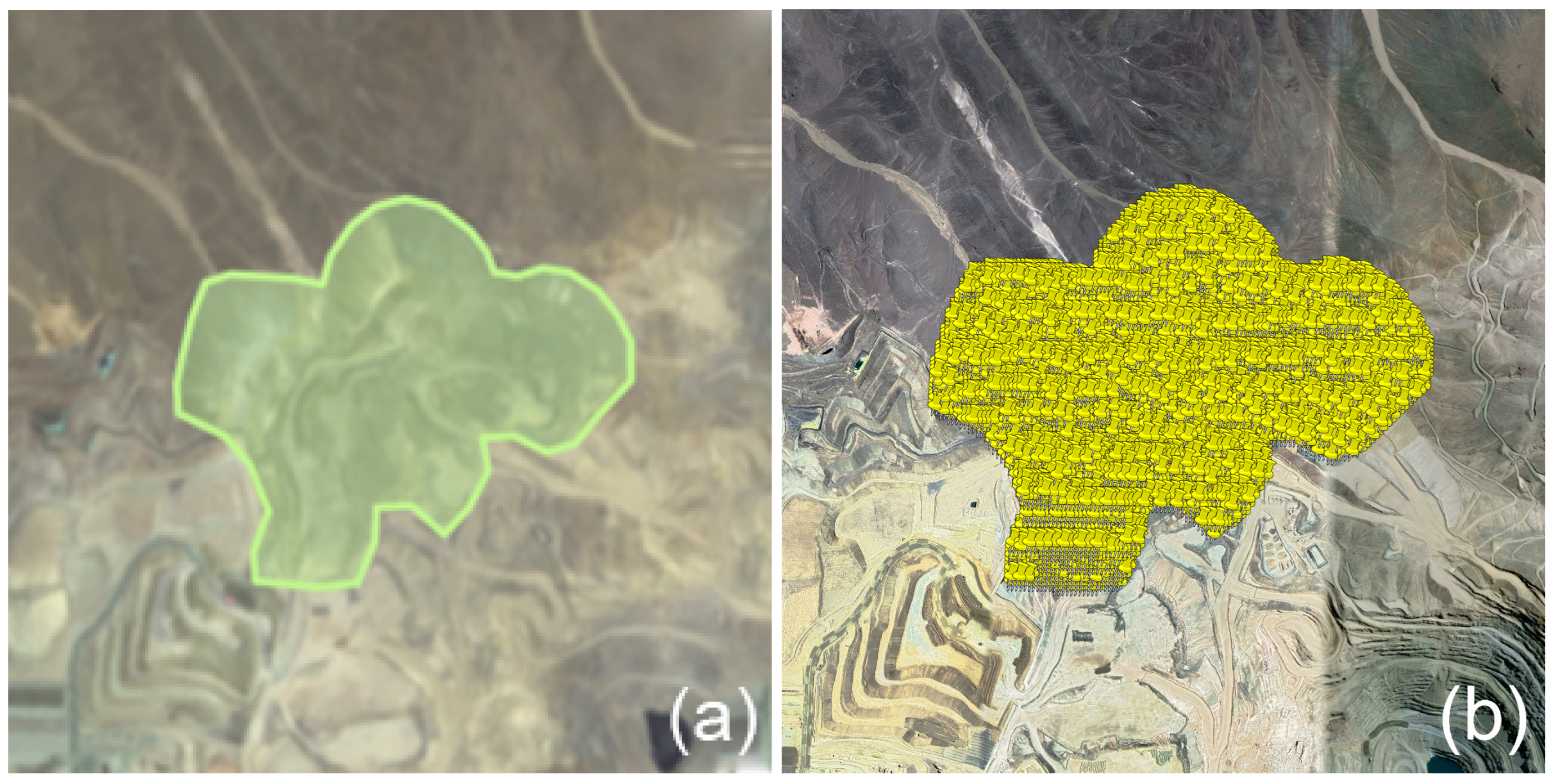
In the global mining sector, addressing the management and monitoring of massive mining waste deposits (MWDs) is critical, especially in countries like Chile, which leads in copper production worldwide [1,2,3,4,5]. The numerous phases of mining activities in Chile generate a significant amount of waste, which is stored in various forms such as tailing dams, waste rock dumps (WRDs, Figure 1a), and leaching waste dumps (LWDs, Figure 1b) [1,2,3,4,5]. This waste accumulation poses substantial challenges and requires intricate management and regulatory adherence, particularly during the closure and post-closure stages [6,7,8,9,10].

Figure 1.
Mine waste deposits (MWDs) located in the north region of Chile. (a) Waste rock dump (WRD), (b) Leaching waste dumps (LWDs).
Addressing the challenges related to MWDs is pivotal due to the complexities involved in their management and the limited information available, which impacts entities like SERNAGEOMIN in their regulatory and monitoring roles [11,12]. The varied forms of MWDs, each with their unique characteristics and impacts, necessitate intricate management strategies and strict adherence to national legislation to ensure the safety and well-being of people and the environment [6,7,8,9,10].
The national legislation mandates adherence to the “Methodological Guide for the Evaluation of the Physical Stability of Remaining Mining Facilities” provided by SERNAGEOMIN [11]. This guide outlines the comprehensive methodologies and parameters for evaluating the potential failure mechanisms of MWDs, thereby optimizing the time, cost, and efficacy of physical stability (PS) studies and facilitating streamlined regulatory compliance and approval processes for closure [11].
The integration of satellite imagery, specifically from the Copernicus Sentinel series by ESA [13], and AI technologies offers advanced, innovative solutions in a variety of fields, including vegetation monitoring [14], urban planning [15], and land use classification [16].
This research aims to harness the capabilities of AI and Sentinel-2 satellite imagery to bridge the existing information gaps regarding the PS of MWDs during their closure and post-closure stages [11]. The objective is to create a comprehensive system for maintaining a national record of MWDs, enabling the extraction of crucial variables related to their PS through advanced DL algorithms such as image classification, deep generative models, and object detection. The innovative application of AI in analyzing satellite imagery for the detection and identification of MWDs is a significant advancement in the field, contributing to the establishment of a detailed, accurate national record of MWDs.
By providing a nuanced understanding of MWDs and their associated risks, this methodology supports the advancement of industry standards and regulatory frameworks. It aids entities like SERNAGEOMIN in their inspection and monitoring roles, enabling precise identification of MWD locations and condition assessments and facilitating risk-based prioritization and compliance processes, thereby enhancing operational and environmental safety protocols in the mining sector [11].
2. Related Works
In this section, a review of the literature most relevant to the research of this article is carried out. In particular, different works on satellite image classification, the use of deep generative models, and detection and segmentation algorithms for satellite images are detailed.
2.1. Image Classification
Image classification is a widely used technique for assigning predefined class labels to digital images based on their visual content. In the context of land classification, this technique can be used to automatically identify and map different land cover types, such as forests, croplands, urban areas, and water bodies, from satellite imagery. There are various popular image classification algorithms that are used in practice, including convolutional neural networks (CNNs) [17,18], support vector machines (SVMs) [19,20], and vision transformers (ViT) [21,22]. Each of these algorithms has their own unique strengths and weaknesses, and they have been shown to generalize well to unseen data. For our work, we considered as relevant the following studies that utilize the DL techniques mentioned previously. For instance, ref. [23] examines advancements in DL techniques for agricultural tasks such as plant disease detection, crop/weed discrimination, fruit counting, and land cover classification. Future directions for AI in agriculture are presented, emphasizing the potential of DL-based models to improve automation in the industry. In [24], a remote-sensing scene-classification method using vision transformers is proposed, resulting in high accuracy on various datasets. In [25], a lightweight ConvNet, MSDF-Net, is presented for aerial scene classification with competitive performance and reduced parameters. In [26], a new method, E-ReCNN, is presented for fine-scale change detection in satellite imagery, with improved results compared to other semi-supervised methods and with the potential for global application once trained.
2.2. Deep Generative Models
DGMs can improve DL models’ performance and robustness when labeled data are scarce by generating synthetic data to augment the training dataset. These models can also generate new samples similar to real data, which is useful for data-intensive applications such as medical imaging and computer vision. Additionally, DGMs can be used to generate synthetic data when real-world data collection is difficult or costly.
The use of DGMs has been proposed for various medical and mining applications. In [27], researchers present a study on using GANs [28] for data augmentation in computed tomography segmentation tasks, showing that using CycleGAN [29] improves the performance of a U-Net model. In [30], the authors explore the use of the Stable Diffusion [31] model for generating synthetic medical images, finding that fine-tuning the U-Net [32] component can generate high-fidelity images. In [33], a method using AI algorithms and GANs was proposed to increase the number of samples for studying the PS of tailing dams in mining applications, resulting in an average F1-score of 97%. These studies highlight the potential of DGMs in expanding limited datasets and improving performance in various fields.
2.3. Image Detection and Segmentation
Image detection and segmentation for satellite imagery is a critical task in remote sensing, with applications such as land-use mapping and change detection. Recent techniques in the field are based on DL, specifically CNNs, which have shown superior performance compared to traditional methods. Popular algorithms for image detection and segmentation include RetinaNet [34], Mask R-CNN [35], and U-Net [32], each with their own advantages.
The authors of [36] investigate the use of CNNs for classifying and segmenting satellite orthoimagery and find that CNNs can achieve results comparable to state-of-the-art methods. Ref. [37] applies DL to detect and classify mines and tailing dams in Brazil using satellite imagery, demonstrating potential for low-cost, high-impact data science tools. Ref. [38] proposes a framework using YOLOv4 [39] and random forest [40] algorithms to extract tailings pond margins from high spatial resolution remote sensing images with high accuracy and efficiency. Ref. [41] presents a method for semantic segmentation of high-resolution satellite images using tree-based CNNs, which outperforms other techniques in terms of classification performance and execution time and which suggests that incorporating data augmentation techniques and deeper neural networks in future work could enhance the efficiency of the method.
This study proposes an innovative method for the precise localization, detection, and segmentation of MWDs in Chilean mining facilities. What sets this method apart from previous studies is the use of cutting-edge DL techniques such as YOLOv7, the ViT classifier, and generative models, which have not been applied before in this context. In addition, this study utilizes open access tools to obtain MWD information, making it cost-effective and accessible to other researchers and mining companies. The proposed method also addresses a current challenge in the Chilean mining context, which is the lack of accurate information in the area of MWDs. By leveraging the generated synthetic tiles of MWDs using deep generative models and the ViT classifier, this study is able to estimate the area of detected MWDs, which is a crucial factor in evaluating mining activities. Overall, this study provides a novel and practical approach to the characterization and assessment of MWDs, which can significantly improve safety and operational efficiency in the mining industry.
3. Methodology
The research methodology is outlined in two stages. Stage one involves the acquisition of satellite image datasets, while stage two encompasses tasks for detection, segmentation, and area estimation. Subsequently, a comprehensive explanation of the relevant metrics used to evaluate the models is provided.
3.1. Dataset Creation
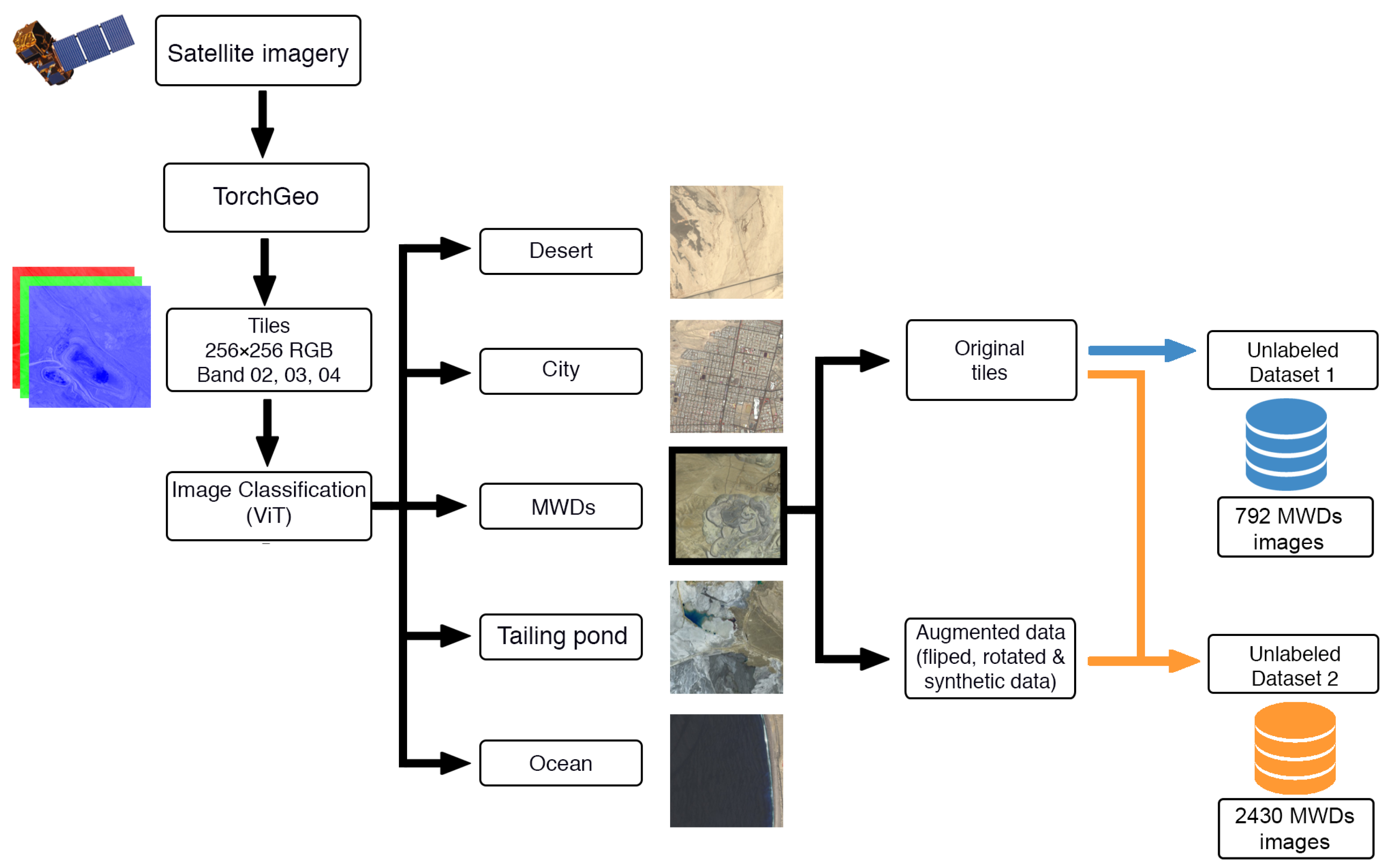
The methodology employed for acquiring the dataset utilized in this research is described in Figure 2. The process consists of four distinct stages: (a) retrieval of satellite imagery from the European Space Agency’s Copernicus Open Access Hub platform and subsequent processing utilizing TorchGeo v0.4.1 [42] to facilitate image analysis; (b) implementation of vision transformer (ViT) techniques for image classification; (c) utilization of deep generative models to generate synthetic maps, thereby augmenting the number of samples in the dataset; and (d) making the prepared dataset available for subsequent analytical stages.
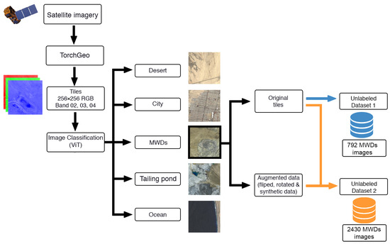
Figure 2.
Methodology applied to obtain satellite imagery from the European Space Agency’s (ESA) Copernicus site to create datasets for conducting experiments.
3.1.1. Satellite Imagery Acquisition
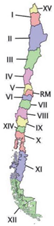
The areas of interest for the study were determined through the identification of the major mining facilities within the country, as sourced from the website of the National Mining Council of Chile [43] and depicted in Table 1. A total of 30 mining facilities were identified and used as a basis for the study.

Table 1.
Major mining facilities in Chile. Figure adapted from [44].
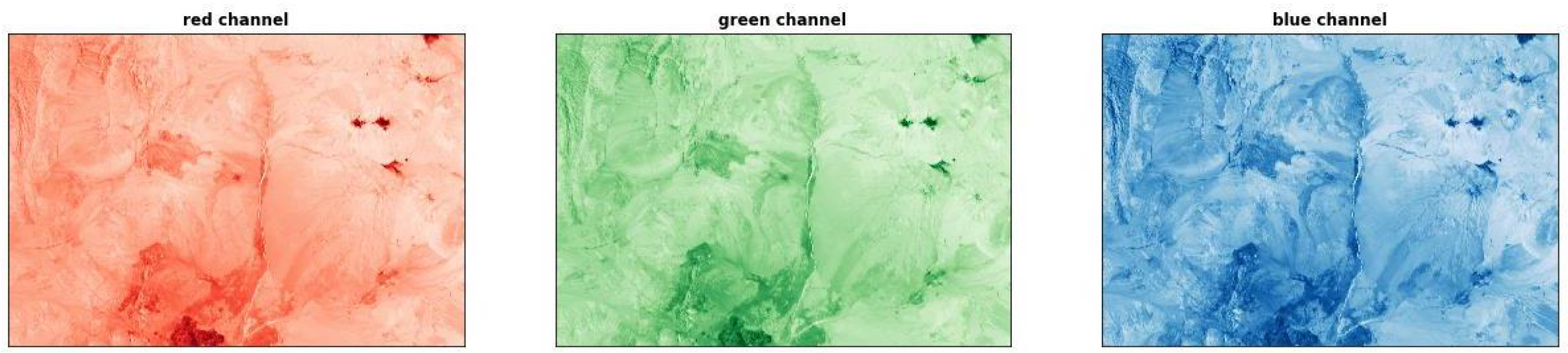
The acquisition of satellite imagery was conducted through the Copernicus Open Access Hub, a platform that provides access to Sentinel data through an interactive graphical user interface. To ensure a high-quality dataset, only products (data items for satellite imagery [44]) with a cloud cover percentage of less than 9% were selected from the Sentinel-2A and Sentinel-2B platforms and S2MSI2A products with bottom-of-atmosphere reflectance. The products were downloaded within the time frame of 2019 to 2022 in SENTINEL-SAFE [45] format. The RGB bands (bands 02, 03, and 04; see Figure 3) were combined into a single image and then segmented into 256 × 256 pixel resolution tiles, with a 20% overlap on adjacent tiles, using the TorchGeo [42] software, for a 10 m spatial resolution. The metadata of the downloaded products were used to determine the vertices in decimal format coordinates in the resulting tiles, and this process was repeated for each of the determined zones.

Figure 3.
Different satellite image bands of the Chuquicamata mining facility (Region II, Antofagasta, Chile). From left to right are the red, green, and blue bands, respectively.
3.1.2. Image Classification
Once the tiles from the mining facilities in Table 1 were obtained, and given the 1:159 relationship of tiles containing MWDs, a ViT image classifier was employed to select the MWD regions for analysis. The images were then categorized into five classes, namely city, desert, sea, tailings pond, and MWD, with each class consisting of 2200 images. This selection was made based on the most frequently occurring scenes from the analysis.
ViT utilizes self-attention mechanisms and the transformer architecture for learning spatial hierarchies of features without image-specific biases. This study adopted the approach of splitting images into positional embedding patches processed by the transformer encoder, which has proven to be highly effective. The results show the effectiveness of the ViT architecture in this context.
To improve performance and prevent overfitting, the selected images were augmented through horizontal and vertical flips and rotations of 90° and −90°, with each class containing 2200 images, including augmentations.
3.1.3. Data Augmentation
Data augmentation is a technique used to artificially increase the size of a dataset in DL and computer vision by applying various random transformations to the existing data, such as rotation, scaling, and flipping. This technique can improve the robustness and generalization of models by exposing them to different variations of the same data. Additionally, it can help to mitigate overfitting by providing the model with more diverse examples.
The procedure was carried out in two phases. The first phase was applied to the ViT classifier, while the second phase was applied to the original 769 MWD image dataset (Figure 4a). For both phases, two augmentations were employed: horizontal flip (Figure 4b) and −90° rotation (Figure 4c).
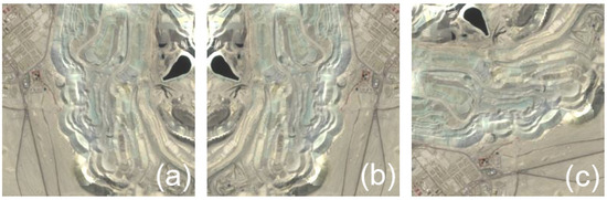
Figure 4.
(a) Original MWD image used for data augmentation, (b) original image flipped horizontally, and (c) original image rotated −90°.
3.1.4. Deep Generative Model
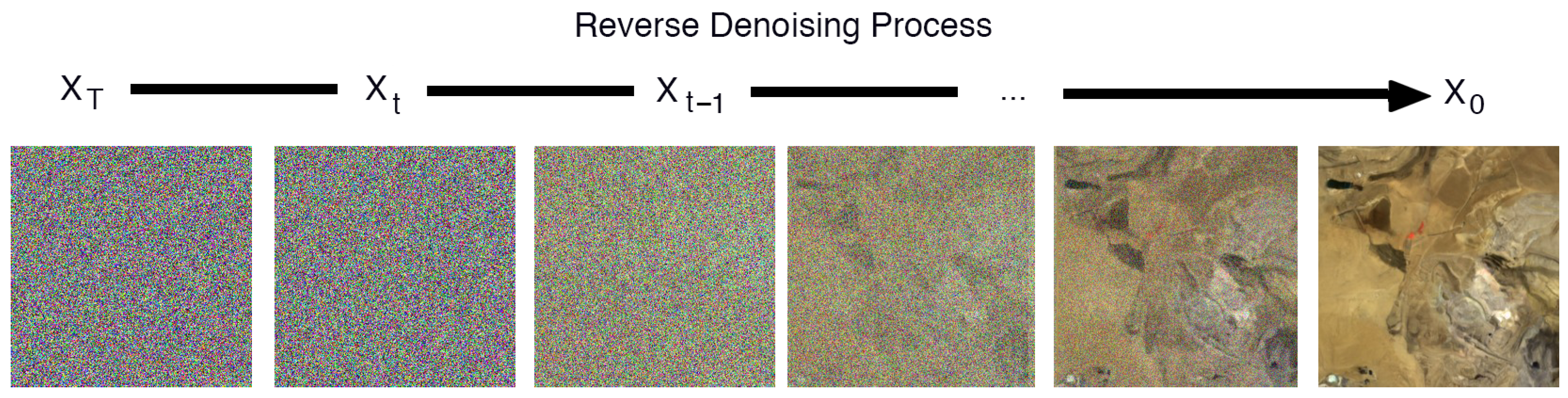
For the generation of synthetic images of maps containing MWDs, we propose a pipeline based on denoising diffusion probabilistic models (DDPMs) [46]. The basic idea behind diffusion models is quite simple. They take the input image and gradually add Gaussian noise through a series of T steps (direct diffusion process). Subsequently, a neural network is trained to recover the original data by inverting the noise process. By modeling the inverse process, we can generate new data. This is called the inverse diffusion process or, in general, the sampling process of a generative model (see Figure 5).
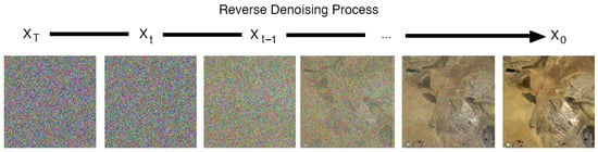
Figure 5.
Reverse denoising process applied to generate a synthetic sample of MWDs.
The process is formulated using a Markov chain consisting of T steps, where each step depends solely on the previous one, a moderate assumption in diffusion models. Most diffusion models use architectures that are some variant of U-Net. The forward diffusion process executed at training is given by Equation (1):
This approach is useful as DDPMs are able to generate high-resolution images, preserving fine details and textures, making it suitable for data augmentation. This is essential for our application of generating synthetic maps containing MWD zones. As we saw in the previous stage, the ViT classifier is utilized to detect the patches corresponding to MWDs. The images classified as MWDs are then utilized as input to train the DDPM algorithm, using unconditional guidance. In our implementation, we train a DDPM model with a database of 792 MWD images. A U-Net architecture is used for the image denoising, configured with two ResNet layers for each U-Net block, with identical input and output channels corresponding to 3 channels for RGB and a resolution of 256 × 256 pixels. The noise scheduler process is configured to 1000 steps in order to add noise to the images.
3.1.5. Unlabeled Dataset
The images were arranged in preparation for the subsequent stage of locating, detecting, and segmenting MWDs. The images are assembled into two datasets as the final step of the procedure outlined in Figure 2 to perform the different experiments. These correspond to:
- Unlabeled Dataset 1. Original dataset containing 792 MWD images.
- Unlabeled Dataset 2. Original dataset plus increased data as described in data augmentation and synthetic MWDs tiles, totaling 2430 MWD images.
The composite image in Figure 6 displays the tiles (centered in the Centinela mining facility) that make up the dataset, showcasing the 20% overlap used. The image consists of unlabeled images.
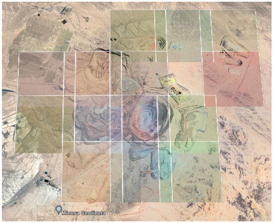
Figure 6.
Representation of the detected MWD-containing tiles superimposed on Google Earth in the Centinela mining facility, Region II, Antofagasta, Chile.
3.2. Detection and Segmentation of MWDs
Once the various image datasets have been obtained and arranged, the second part of the methodology enables detection, segmentation, and estimation of the areas of MWDs. This methodology is shown in Figure 7, where the following steps are observed: (a) the two obtained datasets are labeled with human-annotated labels for the MWD regions within each dataset; (b) the two datasets are then used to train three experiments with detection and segmentation algorithms; and (c) compute the surface area measurements based on the outputs of the detection and segmentation algorithms.
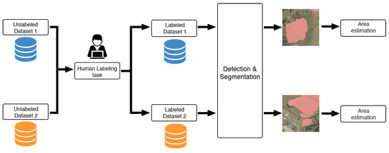
Figure 7.
Methodology employed for the detection, segmentation, and calculation of the area of MWDs.
3.2.1. Human-Annotated Labels
In DL, human-annotated labels, which include object or image classes, bounding box coordinates, and other attributes, are used to train and evaluate machine learning models. Image classification recognizes objects and properties within an image, while object detection localizes objects through bounding boxes. Image segmentation allows for understanding of an image at the pixel level, with semantic segmentation assigning each pixel to a single class. In this research, the use of segmentation masks is employed to achieve the proposed objectives and application. The masks are labeled using Label Studio [47] software v1.5.0. The labels are confirmed by an expert who recognizes MWDs based on the geographical location of the mining facility and the characteristics of the MWDs, such as the distance from the mining pit, texture and color of the mine waste, the shape, and geometry. This process is repeated for all available datasets.
3.2.2. Detection and Segmentation of MWDs
Two segmentation algorithms were tested for extracting features from manually labeled tiles containing MWDs, resulting in 792 zones. The first algorithm is YOLOv7 [48], developed by Wong Kin-Yiu and Alexey Bochkovskiy, a state-of-the-art model for object detection and instance segmentation.
YOLOv7 is built upon the Efficient Layer Aggregation Network (ELAN) [49], optimizing several parameters and computational densities to design an efficient network, and is specifically extended to E-ELAN for more substantial learning ability. E-ELAN enhances the model’s learning capability by using group convolution to expand the channels and cardinality of the computational block and by applying the same channel multiplier and group parameter to all the computational blocks in a computation layer. This model preserves the architecture of the transition layer while modifying the computational block in ELAN. The enhancements lead to the improvement of gradient flow paths and an increase in diverse feature learning, contributing to faster and more accurate inferences.
YOLOv7 employs advanced model scaling techniques, which are crucial for adjusting the model’s depth, image resolution, and width to meet various application requirements. These adjustments are meticulously done to maintain the optimal structure and the initial properties of the architecture, even when concatenating with other layers.
In this study, the YOLOv7 pre-trained model was utilized with its default architecture. The chosen hyperparameters, including epochs, batch size, learning rate, and input image size, are described in Table 2. The image data were normalized and distributed into training (70%), validation (20%), and testing (10%) subsets to ensure a balanced evaluation.
Table 2.
Hyperparameters used in the detection and segmentation stages.
The second algorithm is Mask R-CNN [35], another advanced object instance segmentation model that extends Faster R-CNN [50] by adding a fully convolutional network to predict object masks in parallel with bounding box and class predictions. For Mask R-CNN, two different backbones, namely ResNet50 and ResNet101 [51] from the Detectron2 [52] library, were employed, with fine-tuning performed on both configurations. The hyperparameters for these experiments are also detailed in Table 2, providing a consolidated view of the training configurations for both segmentation algorithms.
3.2.3. Area Estimation
Once the models were trained and their evaluation metrics obtained, they were applied to unseen images to make predictions regarding object detection and segmentation. This was done using tiles generated from RGB bands at 10 m of spectral resolution, with each pixel in the image representing a 10 m × 10 m square on the ground. Information on vertex coordinates in decimal format was also available from the tile generation process. By utilizing the fact that the image always has a resolution of 256 × 256 pixels, it was possible to establish a correlation between the identified mask and its representation in decimal format coordinates.
The calculation of the MWD area was performed using the Gaussian area formula. The area of the polygon P with vertices , , …, is calculated using the Gaussian area formula, as shown in Equation (2).
Furthermore, the Google Earth (GE) API [53] can be employed to calculate the area of a polygon through its coordinates. This enables a comparison between the estimated area obtained through a mathematical approach and the measurements obtained through the API. The GE API is utilized to corroborate the results obtained, thereby obtaining verified values.
3.3. Evaluation Metrics
Evaluating the performance of the algorithms employed in this experiment requires an understanding of relevant metrics.
3.3.1. Metrics for Classification, Detection, and Segmentation
The most commonly used metrics for evaluating image classification, detection, and segmentation models are precision, recall, F1-score, accuracy, macro AVG, and weighted AVG.
where —true positive, —true negative, —false positive, and —false negative. Precision (Equation (3)) measures the proportion of true positive detections among all positive detections made by the model. Recall (Equation (4)) measures the proportion of true positive detections among all actual positive instances in the dataset. F1-score (Equation (5)) is the harmonic mean of precision and recall. Accuracy (Equation (6)) is a measure of the model’s overall performance, calculated as the proportion of correct predictions out of all predictions.
Additionally, for image detection and segmentation performance evaluation, the use of intersection over union (IoU) and mean average precision (mAP) are also considered relevant metrics in this context.
IoU (Equation (7)) is a metric used to evaluate the accuracy of image segmentation models by comparing the overlap between the predicted and ground truth segments. mAP (Equation (8)) is a measure of the model’s overall performance, used to measure the average precision of all classes by taking into account both true positive and false positive detections.
3.3.2. Metrics for Deep Generative Models
The Fréchet inception distance (FID) [54] is a method for evaluating the quality of images generated by generative models. It compares the statistics of the generated images to those of real images by measuring the Fréchet distance between the Inceptionv3 [55] features of the two distributions. The lower the FID score, the more similar the generated images are to the real images, indicating a higher quality of the generated images. It has been shown to correlate well with human judgment of image quality and is widely used in the literature to evaluate the performance of generative models. It is calculated by Equation (9):
where and represent the mean vectors of the feature activation in the Inception network for the real data and generated data, respectively. and represent the covariance matrices of the feature activation in the Inception network for the real data and generated data, respectively. is the trace operator. is the matrix square root of the product of the two covariance matrices.
4. Experiments and Results
In this section, the results obtained from the methodology presented in the previous section are presented. Initially, the results obtained in creating the two databases will be shown. For this, the results for each relevant stage of the process will be presented. In the second part, the results of the detection and area estimation system will be presented, with a comparison to the GE API.
4.1. Results for Dataset Creation
The creation of the datasets involved the utilization of two deep learning models: the ViT image classifier and the deep generative model, specifically, DDPM.
4.1.1. ViT Classifier
The ViT model utilizes the Transformer architecture to perform image classification. The input image is divided into smaller patches which are then flattened and fed as input sequences to the Transformer model. The Transformer performs self-attention operations on these sequences to capture global context and correlations between patches, ultimately producing a feature representation of the entire image. This representation is then fed through a classifier head to predict the class label of the image.
The ViT image classifier was configured with five balanced classes: desert, city, tailings pond, ocean, and MWD, and each class contained 2200 images. The hyperparameters from the model in [56], pre-trained on ImageNet-21k [57], were used. This model uses 12 attention heads, encoder layer dimensionality and hidden size set to 768, 12 hidden layers, and patches of 16 × 16 resolution. The data were split into training, validation, and testing subsets in ratios of 70%, 20%, and 10%, respectively. The model was trained for 300 epochs with a batch size of 240. The results of the ViT image classifier are presented in Table 3.
Table 3.
ViT classifier results for the experiment proposed in Figure 2 to classify five different types of imagery.
The ViT classifier demonstrated high accuracy, with a result of 98.8%, in differentiating between five scenes of aerial imagery.
4.1.2. Deep Generative Model
The DDPM model was trained using images containing MWDs, with a configuration of 250 epochs and a batch size of 8, at a resolution of 256 × 256 pixels. The original denoising DDPM algorithm was employed to sample images for the model, as it generated the highest number of expert-verified samples of MWDs.
A total of 1125 maps were generated, which were then classified by the ViT classifier to identify those that visually resemble MWDs. Finally, the best 792 tiles were selected. The FID score was computed for 792 real and synthetic images using Equation (9), resulting in a score of 222.46. Potential avenues for improvement of the FID score include the generation of high-quality synthetic data for comparison with the original dataset and the implementation of a more diverse and extensive training set for the DDPM model. The implementation of these proposed solutions has the potential to result in a lower FID score.
The application of the ViT classifier and DDPM resulted in the successful creation of two datasets, composed of 792 and 2430 images of MWDs, respectively.
4.2. Results for Detection, Segmentation, and Area Estimation
This section contains the results of experiments using the application of Mask R-CNN and YOLOv7 detection and segmentation algorithms used for the purpose of estimating the areas of MWDs in satellite imagery. This procedure is repeated for each dataset created. A comprehensive analysis of the procedures and results of the area estimation was conducted using both the segmentation masks and the GE API.
4.2.1. Results for YOLOv7 and Mask R-CNN
The Mask R-CNN and YOLOv7 models were evaluated using a k-fold cross-validation approach with 5 folds. The experiments were performed on the dataset, and the reported results represent the average performance across the folds.
The Mask R-CNN models were configured with two backbone networks, namely ResNet50 and ResNet101, both of which were equipped with FPN for feature extraction, with 3× schedule [58]. Fine-tuning was performed on both configurations, utilizing the respective backbone weights. The experiment was executed with an epoch setting of 3000 and a batch size of 450.
The YOLOv7 model was fine-tuned using the official weights available in its repository, with an epoch set to 3000 and a batch size of 448. In both cases, the images were normalized and partitioned into three subsets, with 70% of the images designated for training, 20% for validation, and 10% for testing purposes, respectively.
The results of the experiments performed using the two generated datasets are presented in Table 4. The table displays the AP metrics for detection (AP box) and segmentation (AP Mask), with the best results emphasized in bold for all experiments performed. The AP calculation was conducted with an IoU of 1.
Table 4.
Results of YOLOv7 and Mask R-CNN algorithms for MWD detection and segmentation.
As can be seen in Table 4, the AP score result for object detection, in all cases, is higher than for object segmentation, but by a small margin. It is observed that increasing the data with data augmentation techniques results in a significant improvement in the performance of MWD detection. Additionally, the YOLOv7 algorithm outperforms Mask R-CNN in all cases, based on its AP score. The disparity in results between YOLO and Mask R-CNN can be attributed to their utilization of distinct architectures. YOLO, a single-shot object detection model, predicts object bounding boxes through the utilization of a grid-based approach [59]. In contrast, Mask R-CNN operates in two stages, utilizing region proposal networks (RPNs) and a mask prediction stage to achieve object segmentation [35]. The differing architectures of the algorithms contribute significantly to their performance, with YOLO’s simpler grid-based approach proving effective for objects with clear boundaries and well-defined shapes, while Mask R-CNN’s more complex architecture excels in handling small or overlapping objects [60], which is not the case for our MWD detection and segmentation.
4.2.2. Results for Area Estimation
The objective of this experiment is to determine the accuracy of the estimated areas obtained from the applied area formula compared to the actual measurements obtained through the GE API.
The detected MWDs were obtained using YOLOv7, where the output of the segmentation model produces a polygonal mask. The Gaussian area formula was used to estimate the area of the identified MWDs. The same detected polygon was used with the GE API to obtain the area with this method.
The estimated areas of 10 random samples of detected MWDs, using both the Gaussian area formula and the GE API, are presented in Table 5.
Table 5.
Areas of the 10 MWD random samples estimated using both the Gaussian area algorithm and the GE API. Subsequently, the absolute error, standard deviation, and variance of the two measurements were calculated.
The average absolute error for the samples in Table 5 was found to be 5.58%, which is within the expected range. Further analysis of 100 detected MWDs revealed an average absolute error in area calculation using our proposed method of 6.6%. While there was a slight increase in error, the results indicate that the performance of our system is highly satisfactory.
To validate the estimated areas using our solution, Figure 8 shows a detected MWD, Figure 8a shows the detected polygon area of size 623,886 , and Figure 8b shows the projection of the area of size 647,681 in Google Earth.

Figure 8.
Detected MWDs using our proposed methodology. (a) shows the mask detected over a tile of Sentinel-2 imagery; (b) shows the same area exported to Google Earth.
The experiments demonstrated that the mathematical approach for estimating the area of MWDs is both accurate and valid, as the estimated area was in agreement with the measurements obtained through the GE API. This approach offers the advantage of providing accurate results while saving time compared to manual measurements. The utilization of the GE API also facilitated easy visualization and verification of the results, further confirming the validity of this approach as an alternative method for estimating the area of MWDs.
5. Conclusions and Future Work
In this study, we introduced a methodology aimed at the localization and estimation of the area of MWDs by employing advanced DL techniques. This methodology aspires to provide a foundational framework for analyzing PS, a crucial aspect during the closure and post-closure phases of mining operations.
Utilizing a ViT classifier, we achieved a classification accuracy of 98% across various aerial scenes. This demonstrates a promising avenue for processing satellite imagery in the context of mining waste management. Additionally, the employment of DGMs proved beneficial in augmenting the limited data available, showcasing a potential path for enhancing detection algorithms.
The application of YOLOv7 and Mask R-CNN algorithms on RGB imagery with a 10 m spectral resolution facilitated the accurate detection and segmentation of MWDs while preserving the location information derived from Sentinel-2 metadata. The experimental results indicate that the combination of YOLOv7 and diffusion models was effective in detecting and segmenting MWDs. Specifically, the YOLOv7 algorithm achieved an AP of 81% for detection and 79% for segmentation when integrating original, augmented, and synthetic data. This suggests that synthetic data can play a role in improving the accuracy of detection algorithms.
Furthermore, the methodology allowed for the estimation of areas of detected MWDs, offering a cost-effective alternative to the challenge of cataloging and accounting for the quantity of MWDs in a region.
The analysis of satellite images corresponding to the MWD areas could potentially provide variables associated with site sector, geomorphology, vegetation, populated sectors, and environmentally protected areas. This lays the groundwork for further exploration into machine learning algorithms for feature extraction, image processing, manual labeling, and deep learning in the context of mining waste management.
While this study presents an initial step towards addressing the challenges associated with the fiscalization process of MWDs, further research is warranted to refine the proposed methodology and explore other machine learning and deep learning algorithms for improved accuracy and efficiency.
Author Contributions
Conceptualization, M.S., G.H., G.V. and P.B.; methodology, M.S., G.H. and G.V.; software, M.S. and G.H.; validation, M.S., G.H. and G.V.; formal analysis, M.S. and G.H.; investigation, M.S., G.H., G.V. and P.B.; resources, P.B., G.V. and G.H.; data curation, M.S.; writing—original draft preparation, M.S.; writing—review and editing, P.B.; visualization, M.S., G.V. and G.H.; supervision, P.B.; project administration, G.V. and G.H.; funding acquisition, G.V., G.H. and P.B. All authors have read and agreed to the published version of the manuscript.
Funding
This research was funded and supported by Agencia Nacional de Investigación y Desarrollo (ANID): (i) grant number FONDEF IT20I0016: Plataforma Inteligente para la Evaluación Periódica de la Estabilidad Física en vista a un Cierre Progresivo y Seguro de Depósitos de Relaves de la Mediana Minería; (ii) grant number MEC 80190075; (iii) ANID Doctorado Nacional 2023-21232328; and DI-PUCV number 039.349/2023.
Data Availability Statement
Not applicable.
Acknowledgments
Our sincere thanks to Servicio Nacional de Geología y Minería (SERNAGEOMIN, Ministerio de Minería, Chile), Ministerio de Educación (Chile), Vicerrectoría de Investigación, Creación e Innovación de la Pontificia Universidad Católica de Valparaíso (Chile).
Conflicts of Interest
The authors declare no conflict of interest.
References
- SERNAGEOMIN Site. Datos Públicos Depósitos de Relaves. Catastro de Depósitos de Relaves en Chile 2022. Available online: https://www.sernageomin.cl/datos-publicosdeposito-de-relaves/ (accessed on 30 January 2023).
- Palma, C.; Linero, S.; Apablaza, R. Geotechnical Characterisation of Waste Material in Very High Dumps with Large Scale Triaxial Testing. In Slope Stability 2007: Proceedings of the 2007 International Symposium on Rock Slope Stability in Open Pit Mining and Civil Engineering; Potvin, Y., Ed.; Australian Centre for Geomechanics: Perth, Australia, 2007; pp. 59–75. [Google Scholar] [CrossRef]
- Valenzuela, L.; Bard, E.; Campaña, J. Seismic considerations in the design of high waste rock dumps. In Proceedings of the 5th International Conference on Earthquake Geotechnical Engineering (5-ICEGE), Santiago, Chile, 10–13 January 2011. [Google Scholar]
- Bard, E.; Anabalón, M.E. Comportement des stériles Miniers ROM à Haute Pressions. Du Grain à l’ouvrage. 2008. Available online: https://www.cfms-sols.org/sites/default/files/manifestations/080312/2-Bard.pdf (accessed on 2 March 2023).
- Fourie, A.; Villavicencio, G.; Palma, J.; Valenzuela, P.; Breul, P. Evaluation of the physical stability of leaching waste deposits for the closure stage. In Proceedings of the 20th International Conference on Soil Mechanics and Geotechnical Engineering, Sydney, Australia, 1–5 May 2022. [Google Scholar]
- Biblioteca del Congreso Nacional de Chile Site. Ley 19300. Ley Sobre Bases Generales del Medio Ambiente. Available online: https://www.bcn.cl/leychile/navegar?idNorma=30667&idParte=9705635&idVersion=2021-08-13 (accessed on 3 February 2023).
- Biblioteca del Congreso Nacional de Chile Site. Decreto Supremo N° 132: Reglamento de Seguridad Minera. Available online: https://www.bcn.cl/leychile/navegar?idNorma=221064 (accessed on 3 February 2023).
- Biblioteca del Congreso Nacional de Chile Site. Ley N° 20.551: Regula el Cierre de Faenas e Instalaciones Mineras. Available online: https://www.bcn.cl/leychile/navegar?idNorma=1032158 (accessed on 3 February 2023).
- Biblioteca del Congreso Nacional de Chile site. Decreto N° 41: Aprueba el Reglamento de la Ley de Cierre de Faenas e Instalaciones Mineras. Available online: https://www.bcn.cl/leychile/navegar?idNorma=1045967&idParte=9314317&idVersion=2020-06-23 (accessed on 3 February 2023).
- Biblioteca del Congreso Nacional de Chile Site. Ley 20.819: Modifica la Ley N° 20.551: Regula el Cierre de Faenas e Instalaciones Mineras. Available online: https://www.bcn.cl/leychile/navegar?i=1075399&f=2015-03-14 (accessed on 3 February 2023).
- SERNAGEOMIN. Guía Metodológica para Evaluación de la Estabilidad Física de Instalaciones Mineras Remanentes. Available online: https://www.sernageomin.cl/wp-content/uploads/2019/06/GUIA-METODOLOGICA.pdf/ (accessed on 24 January 2023).
- Hawley, P.M. Guidelines for Mine Waste Dump and Stockpile Design; CSIRO Publishing: Clayton, NC, USA, 2017; p. 370. [Google Scholar]
- ESA: Sentinel-2 Mission. Available online: https://sentinels.copernicus.eu/web/sentinel/missions/sentinel-2/ (accessed on 25 January 2023).
- McDowell, N.G.; Coops, N.C.; Beck, P.S.; Chambers, J.Q.; Gangodagamage, C.; Hicke, J.A.; Huang, C.; Kennedy, R.; Krofcheck, D.J.; Litvak, M.; et al. Global satellite monitoring of climate-induced vegetation disturbances. Trends Plant Sci. 2015, 20, 114–123. [Google Scholar] [CrossRef] [PubMed]
- Van Etten, A.; Hogan, D.; Manso, J.M.; Shermeyer, J.; Weir, N.; Lewis, R. The Multi-Temporal Urban Development SpaceNet Dataset. In Proceedings of the IEEE/CVF Conference on Computer Vision and Pattern Recognition (CVPR), Nashville, TN, USA, 20–25 June 2021; pp. 6398–6407. [Google Scholar]
- Talukdar, S.; Singha, P.; Mahato, S.; Shahfahad; Pal, S.; Liou, Y.A.; Rahman, A. Land-Use Land-Cover Classification by Machine Learning Classifiers for Satellite Observations—A Review. Remote Sens. 2020, 12, 1135. [Google Scholar] [CrossRef]
- Chen, Y.; Ming, D.; Lv, X. Superpixel based land cover classification of VHR satellite image combining multi-scale CNN and scale parameter estimation. Earth Sci. Inform. 2019, 12, 341–363. [Google Scholar] [CrossRef]
- Spectral Indexes Evaluation for Satellite Images Classification using CNN. J. Inf. Organ. Sci. 2021, 45, 435–449. [CrossRef]
- Lantzanakis, G.; Mitraka, Z.; Chrysoulakis, N. X-SVM: An Extension of C-SVM Algorithm for Classification of High-Resolution Satellite Imagery. IEEE Trans. Geosci. Remote Sens. 2021, 59, 3805–3815. [Google Scholar] [CrossRef]
- Abburu, S.; Golla, S. Satellite Image Classification Methods and Techniques: A Review. Int. J. Comput. Appl. 2015, 119, 20–25. [Google Scholar] [CrossRef]
- Kaselimi, M.; Voulodimos, A.; Daskalopoulos, I.; Doulamis, N.; Doulamis, A. A Vision Transformer Model for Convolution-Free Multilabel Classification of Satellite Imagery in Deforestation Monitoring. IEEE Trans. Neural Netw. Learn. Syst. 2023, 34, 3299–3307. [Google Scholar] [CrossRef]
- Horvath, J.; Baireddy, S.; Hao, H.; Montserrat, D.M.; Delp, E.J. Manipulation Detection in Satellite Images Using Vision Transformer. In Proceedings of the IEEE/CVF Conference on Computer Vision and Pattern Recognition (CVPR) Workshops, Nashville, TN, USA, 20–25 June 2021; pp. 1032–1041. [Google Scholar]
- Saleem, M.H.; Potgieter, J.; Arif, K.M. Automation in Agriculture by Machine and Deep Learning Techniques: A Review of Recent Developments. Precis. Agric. 2021, 22, 2053–2091. [Google Scholar] [CrossRef]
- Bazi, Y.; Bashmal, L.; Rahhal, M.M.A.; Dayil, R.A.; Ajlan, N.A. Vision Transformers for Remote Sensing Image Classification. Remote Sens. 2021, 13, 516. [Google Scholar] [CrossRef]
- Yi, J.; Zhou, B. A Multi-Stage Duplex Fusion ConvNet for Aerial Scene Classification. arXiv 2022, arXiv:2203.16325. [Google Scholar]
- Camalan, S.; Cui, K.; Pauca, V.P.; Alqahtani, S.; Silman, M.; Chan, R.; Plemmons, R.J.; Dethier, E.N.; Fernandez, L.E.; Lutz, D.A. Change Detection of Amazonian Alluvial Gold Mining Using Deep Learning and Sentinel-2 Imagery. Remote Sens. 2022, 14, 1746. [Google Scholar] [CrossRef]
- Sandfort, V.; Yan, K.; Pickhardt, P.J.; Summers, R.M. Data augmentation using generative adversarial networks (CycleGAN) to improve generalizability in CT segmentation tasks. Sci. Rep. 2019, 9, 16884. [Google Scholar] [CrossRef] [PubMed]
- Goodfellow, I.J.; Pouget-Abadie, J.; Mirza, M.; Xu, B.; Warde-Farley, D.; Ozair, S.; Courville, A.; Bengio, Y. Generative Adversarial Networks. arXiv 2014, arXiv:1406.2661. [Google Scholar] [CrossRef]
- Zhu, J.Y.; Park, T.; Isola, P.; Efros, A.A. Unpaired Image-to-Image Translation using Cycle-Consistent Adversarial Networks. arXiv 2017, arXiv:1703.10593. [Google Scholar]
- Chambon, P.; Bluethgen, C.; Langlotz, C.P.; Chaudhari, A. Adapting Pretrained Vision-Language Foundational Models to Medical Imaging Domains. arXiv 2022, arXiv:2210.04133. [Google Scholar]
- Rombach, R.; Blattmann, A.; Lorenz, D.; Esser, P.; Ommer, B. High-Resolution Image Synthesis with Latent Diffusion Models. In Proceedings of the 2022 IEEE/CVF Conference on Computer Vision and Pattern Recognition (CVPR), New Orleans, LA, USA, 18–24 June 2022; pp. 10674–10685. [Google Scholar] [CrossRef]
- Ronneberger, O.; Fischer, P.; Brox, T. U-Net: Convolutional Networks for Biomedical Image Segmentation. arXiv 2015, arXiv:1505.04597. [Google Scholar]
- Pacheco, F.; Hermosilla, G.; Piña, O.; Villavicencio, G.; Allende-Cid, H.; Palma, J.; Valenzuela, P.; García, J.; Carpanetti, A.; Minatogawa, V.; et al. Generation of Synthetic Data for the Analysis of the Physical Stability of Tailing Dams through Artificial Intelligence. Mathematics 2022, 10, 4396. [Google Scholar] [CrossRef]
- Lin, T.Y.; Goyal, P.; Girshick, R.; He, K.; Dollár, P. Focal Loss for Dense Object Detection. arXiv 2017, arXiv:1708.02002. [Google Scholar]
- He, K.; Gkioxari, G.; Dollár, P.; Girshick, R. Mask R-CNN. arXiv 2017, arXiv:1703.06870. [Google Scholar]
- Längkvist, M.; Kiselev, A.; Alirezaie, M.; Loutfi, A. Classification and Segmentation of Satellite Orthoimagery Using Convolutional Neural Networks. Remote Sens. 2016, 8, 329. [Google Scholar] [CrossRef]
- Balaniuk, R.; Isupova, O.; Reece, S. Mining and Tailings Dam Detection in Satellite Imagery Using Deep Learning. arXiv 2020, arXiv:2007.01076. [Google Scholar]
- Lyu, J.; Hu, Y.; Ren, S.; Yao, Y.; Ding, D.; Guan, Q.; Tao, L. Extracting the Tailings Ponds from High Spatial Resolution Remote Sensing Images by Integrating a Deep Learning-Based Model. Remote Sens. 2021, 13, 743. [Google Scholar] [CrossRef]
- Bochkovskiy, A.; Wang, C.Y.; Liao, H.Y.M. YOLOv4: Optimal Speed and Accuracy of Object Detection. arXiv 2020, arXiv:2004.10934. [Google Scholar]
- Breiman, L. Random Forests. Mach. Learn. 2001, 45, 5–32. [Google Scholar] [CrossRef]
- Robinson, Y.H.; Vimal, S.; Khari, M.; Hernández, F.C.L.; Crespo, R.G. Tree-based convolutional neural networks for object classification in segmented satellite images. Int. J. High Perform. Comput. Appl. 2020, 1094342020945026. [Google Scholar] [CrossRef]
- Stewart, A.J.; Robinson, C.; Corley, I.A.; Ortiz, A.; Lavista Ferres, J.M.; Banerjee, A. TorchGeo: Deep Learning with Geospatial Data. In Proceedings of the 30th International Conference on Advances in Geographic Information Systems, Seattle, WA, USA, 1–4 November 2022; pp. 1–12. [Google Scholar] [CrossRef]
- Consejo Minero. Mapa Minero. Available online: https://consejominero.cl/nosotros/mapa-minero/ (accessed on 12 January 2023).
- ESA: Sentinel-2 Overview. Available online: https://sentinel.esa.int/web/sentinel/user-guides/sentinel-2-msi/overview (accessed on 17 January 2023).
- ESA. Data Formats—User Guides—Sentinel-2 MSI—Sentinel Online—Sentinel Online. Available online: https://sentinels.copernicus.eu/web/sentinel/user-guides/sentinel-2-msi/data-formats (accessed on 20 January 2023).
- Ho, J.; Jain, A.; Abbeel, P. Denoising Diffusion Probabilistic Models. arXiv 2020, arXiv:2006.11239. [Google Scholar]
- Tkachenko, M.; Malyuk, M.; Holmanyuk, A.; Liubimov, N. Label Studio: Data Labeling Software, 2020–2022. Available online: https://github.com/HumanSignal/label-studio (accessed on 11 October 2023).
- Wang, C.Y.; Bochkovskiy, A.; Liao, H.Y.M. YOLOv7: Trainable Bag-of-Freebies Sets New State-of-the-Art for Real-Time Object Detectors. arXiv 2022, arXiv:2207.02696. [Google Scholar]
- Zhang, X.; Zeng, H.; Guo, S.; Zhang, L. Efficient Long-Range Attention Network for Image Super-resolution. In Proceedings of the European Conference on Computer Vision, Tel Aviv, Israel, 23–27 October 2022. [Google Scholar]
- Ren, S.; He, K.; Girshick, R.; Sun, J. Faster R-CNN: Towards Real-Time Object Detection with Region Proposal Networks. arXiv 2015, arXiv:1506.01497. [Google Scholar] [CrossRef]
- Szegedy, C.; Ioffe, S.; Vanhoucke, V.; Alemi, A. Inception-v4, Inception-ResNet and the Impact of Residual Connections on Learning. arXiv 2016, arXiv:1602.07261. [Google Scholar] [CrossRef]
- Wu, Y.; Kirillov, A.; Massa, F.; Lo, W.Y.; Girshick, R. Detectron2. 2019. Available online: https://github.com/facebookresearch/detectron2 (accessed on 11 October 2023).
- Gorelick, N.; Hancher, M.; Dixon, M.; Ilyushchenko, S.; Thau, D.; Moore, R. Google Earth Engine: Planetary-Scale Geospatial Analysis for Everyone; Elsevier: Amsterdam, The Netherlands, 2017. [Google Scholar] [CrossRef]
- Heusel, M.; Ramsauer, H.; Unterthiner, T.; Nessler, B.; Hochreiter, S. GANs Trained by a Two Time-Scale Update Rule Converge to a Local Nash Equilibrium. arXiv 2017, arXiv:1706.08500. [Google Scholar]
- Szegedy, C.; Vanhoucke, V.; Ioffe, S.; Shlens, J.; Wojna, Z. Rethinking the Inception Architecture for Computer Vision. arXiv 2015, arXiv:1512.00567. [Google Scholar]
- Hugging Face. Google/Vit-Base-Patch16-224. Available online: https://huggingface.co/google/vit-base-patch16-224 (accessed on 30 January 2023).
- Ridnik, T.; Ben-Baruch, E.; Noy, A.; Zelnik-Manor, L. ImageNet-21K Pretraining for the Masses. arXiv 2021, arXiv:2104.10972. [Google Scholar]
- He, K.; Girshick, R.; Dollár, P. Rethinking ImageNet Pre-training. arXiv 2018, arXiv:1811.08883. [Google Scholar]
- Redmon, J.; Divvala, S.; Girshick, R.; Farhadi, A. You Only Look Once: Unified, Real-Time Object Detection. arXiv 2015, arXiv:1506.02640. [Google Scholar]
- Girshick, R.B.; Donahue, J.; Darrell, T.; Malik, J. Rich feature hierarchies for accurate object detection and semantic segmentation. arXiv 2013, arXiv:abs/1311.2524. [Google Scholar]


Disclaimer/Publisher’s Note: The statements, opinions and data contained in all publications are solely those of the individual author(s) and contributor(s) and not of MDPI and/or the editor(s). MDPI and/or the editor(s) disclaim responsibility for any injury to people or property resulting from any ideas, methods, instructions or products referred to in the content. |
© 2023 by the authors. Licensee MDPI, Basel, Switzerland. This article is an open access article distributed under the terms and conditions of the Creative Commons Attribution (CC BY) license (https://creativecommons.org/licenses/by/4.0/).