
Learn to Few-Shot Segment Remote Sensing Images from Irrelevant Data
 ,
,
Abstract
:
1. Introduction
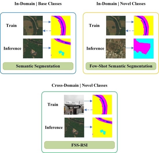
- We extend the FSS to FSS-RSI, which aims to utilize irrelevant domain data to guide the segmentation of remote sensing images.
- A new benchmark is proposed. This benchmark may promote the development of FSS-RSI and serve as a tool for researchers.
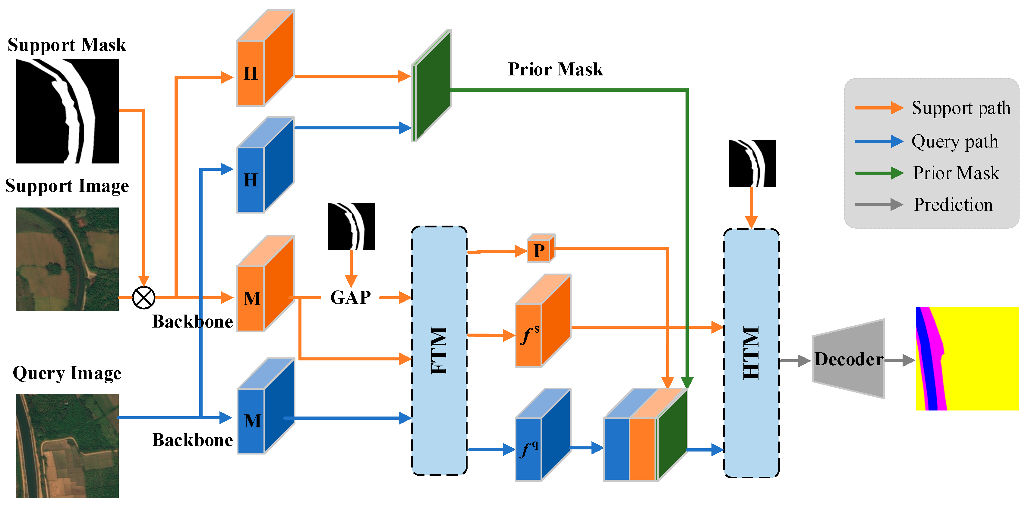
- We propose an effective network with the FTM and the HTM. Our method significantly outperforms the cutting-edge few-shot semantic segmentation method in the FSS-RSI task.
2. Method
2.1. Problem Setting
2.2. Model
2.2.1. Feature Extraction
2.2.2. Feature Transformation Module
2.2.3. Hierarchical Transformer Module
2.2.4. Extension to K-Shot
2.3. Benchmark
2.4. Experiments
2.4.1. Datasets and Metric
2.4.2. Training and Testing Strategy
3. Result
3.1. Models for Comparison
3.2. Main Results
4. Discussion
4.1. Ablation Study
4.2. Limitations
5. Conclusions
Author Contributions
Funding
Data Availability Statement
Conflicts of Interest
Appendix A
Appendix B
Appendix C

| Method | Fold0 | Fold1 | Fold2 | Fold3 | Average |
|---|---|---|---|---|---|
| PFENet | 63.23 | 70.79 | 53.28 | 57.25 | 61.14 |
| RPMMs | 59.50 | 71.58 | 55.40 | 51.96 | 59.61 |
| HSNet | 63.03 | 69.50 | 59.64 | 59.88 | 63.01 |
| BAM | 60.94 | 70.75 | 61.77 | 59.45 | 63.23 |
| HDMNet | 66.92 | 75.83 | 67.79 | 69.37 | 69.98 |
| FTNet | 62.42 | 71.06 | 58.00 | 58.91 | 62.60 |
References
- Wang, Z.; Wang, B.; Zhang, C.; Liu, Y.; Guo, J. Defending against Poisoning Attacks in Aerial Image Semantic Segmentation with Robust Invariant Feature Enhancement. Remote Sens. 2023, 15, 3157. [Google Scholar] [CrossRef]
- He, Y.; Jia, K.; Wei, Z. Improvements in Forest Segmentation Accuracy Using a New Deep Learning Architecture and Data Augmentation Technique. Remote Sens. 2023, 15, 2412. [Google Scholar] [CrossRef]
- Shelhamer, E.; Long, J.; Darrell, T. Fully Convolutional Networks for Semantic Segmentation. IEEE Trans. Pattern Anal. Mach. Intell. 2017, 39, 640–651. [Google Scholar] [CrossRef]
- Noh, H.; Hong, S.; Han, B. Learning Deconvolution Network for Semantic Segmentation. In Proceedings of the 2015 IEEE International Conference on Computer Vision (ICCV), Piscataway, NJ, USA, 7–13 December 2015; pp. 1520–1528. [Google Scholar] [CrossRef]
- Badrinarayanan, V.; Kendall, A.; Cipolla, R. SegNet: A Deep Convolutional Encoder-Decoder Architecture for Image Segmentation. IEEE Trans. Pattern Anal. Mach. Intell. 2017, 39, 2481–2495. [Google Scholar] [CrossRef]
- Lin, G.; Milan, A.; Shen, C.; Reid, I. RefineNet: Multi-path Refinement Networks for High-Resolution Semantic Segmentation. In Proceedings of the 2017 IEEE Conference on Computer Vision and Pattern Recognition (CVPR), Honolulu, HI, USA, 21–26 July 2017; pp. 5168–5177. [Google Scholar] [CrossRef]
- Ronneberger, O.; Fischer, P.; Brox, T. U-Net: Convolutional Networks for Biomedical Image Segmentation. arXiv 2015, arXiv:1505.04597. [Google Scholar]
- Yu, F.; Koltun, V. Multi-Scale Context Aggregation by Dilated Convolutions. arXiv 2016, arXiv:1511.07122. [Google Scholar]
- Chen, L.; Papandreou, G.; Kokkinos, I.; Murphy, K.; Yuille, A.L. DeepLab: Semantic Image Segmentation with Deep Convolutional Nets, Atrous Convolution, and Fully Connected CRFs. IEEE Trans. Pattern Anal. Mach. Intell. 2018, 40, 834–848. [Google Scholar] [CrossRef]
- He, K.; Zhang, X.; Ren, S.; Sun, J. Deep Residual Learning for Image Recognition. In Proceedings of the IEEE Conference on Computer Vision and Pattern Recognition, Las Vegas, NV, USA, 27–30 June 2016; pp. 770–778. [Google Scholar] [CrossRef]
- Simonyan, K.; Zisserman, A. Very Deep Convolutional Networks for Large-Scale Image Recognition. arXiv 2014, arXiv:1409.1556. [Google Scholar]
- Dosovitskiy, A.; Beyer, L.; Kolesnikov, A.; Weissenborn, D.; Zhai, X.; Unterthiner, T.; Dehghani, M.; Minderer, M.; Heigold, G.; Gelly, S.; et al. An Image is Worth 16x16 Words: Transformers for Image Recognition at Scale. arXiv 2020, arXiv:2010.11929. [Google Scholar]
- Zheng, S.; Lu, J.; Zhao, H.; Zhu, X.; Luo, Z.; Wang, Y.; Fu, Y.; Feng, J.; Xiang, T.; Torr, P.H.S.; et al. Rethinking Semantic Segmentation from a Sequence-to-Sequence Perspective with Transformers. In Proceedings of the 2021 IEEE/CVF Conference on Computer Vision and Pattern Recognition (CVPR), Nashville, TN, USA, 20–25 June 2021; pp. 6877–6886. [Google Scholar] [CrossRef]
- Xie, E.; Wang, W.; Yu, Z.; Anandkumar, A.; Alvarez, J.M.; Luo, P. SegFormer: Simple and Efficient Design for Semantic Segmentation with Transformers. arXiv 2016, arXiv:2105.15203. [Google Scholar]
- Devlin, J.; Chang, M.-W.; Lee, K.; Toutanova, K. BERT: Pre-training of Deep Bidirectional Transformers for Language Understanding. arXiv 2016, arXiv:1810.04805. [Google Scholar]
- Vaswani, A.; Shazeer, N.; Parmar, N.; Uszkoreit, J.; Jones, L.; Gomez, A.N.; Kaiser, L.; Polosukhin, I. Attention Is All You Need. arXiv 2017, arXiv:1706.03762. [Google Scholar]
- Shaban, A.; Bansal, S.; Liu, Z.; Essa, I.; Boots, B. One-Shot Learning for Semantic Segmentation. arXiv 2017, arXiv:1709.03410. [Google Scholar]
- Tian, Z.; Zhao, H.; Shu, M.; Yang, Z.; Li, R.; Jia, J. Prior Guided Feature Enrichment Network for Few-Shot Segmentation. IEEE Trans. Pattern Anal. Mach. Intell. 2022, 44, 1050–1065. [Google Scholar] [CrossRef] [PubMed]
- Lang, C.; Cheng, G.; Tu, B.; Han, J. Learning What Not to Segment: A New Perspective on Few-Shot Segmentation. In Proceedings of the 2022 IEEE/CVF Conference on Computer Vision and Pattern Recognition (CVPR), New Orleans, LA, USA, 18–24 June 2022; pp. 8047–8057. [Google Scholar] [CrossRef]
- Vinyals, O.; Blundell, C.; Lillicrap, T.; Kavukcuoglu, K.; Wierstra, D. Matching Networks for One Shot Learning. arXiv 2016, arXiv:1606.04080. [Google Scholar]
- Wang, K.; Liew, J.H.; Zou, Y.; Zhou, D.; Feng, J. PANet: Few-Shot Image Semantic Segmentation with Prototype Alignment. In Proceedings of the 2019 IEEE/CVF International Conference on Computer Vision (ICCV), Seoul, Republic of Korea, 27 October–2 November 2019; pp. 9196–9205. [Google Scholar] [CrossRef]
- Zhang, C.; Lin, G.; Liu, F.; Yao, R.; Shen, C. CANet: Class-Agnostic Segmentation Networks With Iterative Refinement and Attentive Few-Shot Learning. In Proceedings of the 2019 IEEE/CVF Conference on Computer Vision and Pattern Recognition (CVPR), Long Beach, CA, USA, 15–20 June 2019; pp. 5212–5221. [Google Scholar] [CrossRef]
- Yang, B.; Liu, C.; Li, B.; Jiao, J.; Ye, Q. Prototype Mixture Models for Few-shot Semantic Segmentation. arXiv 2020, arXiv:2008.03898. [Google Scholar]
- Min, J.; Kang, D.; Cho, M. Hypercorrelation Squeeze for Few-Shot Segmenation. In Proceedings of the 2021 IEEE/CVF International Conference on Computer Vision (ICCV), Montreal, QC, Canada, 10–17 October 2021; pp. 6921–6932. [Google Scholar] [CrossRef]
- Siam, M.; Oreshkin, B. Adaptive Masked Weight Imprinting for Few-Shot Segmentation. arXiv 2019, arXiv:1902.11123. [Google Scholar]
- Peng, B.; Tian, Z.; Wu, X.; Wang, C.; Liu, S.; Su, J.; Jia, J. Hierarchical Dense Correlation Distillation for Few-Shot Segmentation. arXiv 2023, arXiv:2303.14652. [Google Scholar]
- Zhang, G.; Kang, G.; Yang, Y.; Wei, Y. Few-Shot Segmentation via Cycle-Consistent Transformer. arXiv 2021, arXiv:2106.02320. [Google Scholar]
- Zhang, J.; Liu, Y.; Wu, P.; Shi, Z.; Pan, B. Mining Cross-Domain Structure Affinity for Refined Building Segmentation in Weakly Supervised Constraints. Remote Sens. 2022, 14, 1227. [Google Scholar] [CrossRef]
- Gao, H.; Zhao, Y.; Guo, P.; Sun, Z.; Chen, X.; Tang, Y. Cycle and Self-Supervised Consistency Training for Adapting Semantic Segmentation of Aerial Images. Remote Sens. 2022, 14, 1527. [Google Scholar] [CrossRef]
- Sun, L.; Cheng, S.; Zheng, Y.; Wu, Z.; Zhang, J. SPANet: Successive Pooling Attention Network for Semantic Segmentation of Remote Sensing Images. IEEE J. Sel. Top. Appl. Earth Obs. Remote. Sens. 2022, 15, 4045–4057. [Google Scholar] [CrossRef]
- Chen, Y.; Wei, C.; Wang, D.; Ji, C.; Li, B. Semi-Supervised Contrastive Learning for Few-Shot Segmentation of Remote Sensing Images. Remote Sens. 2022, 14, 4254. [Google Scholar] [CrossRef]
- Deng, R.; Shen, C.; Liu, S.; Wang, H.; Liu, X. Learning to Predict Crisp Boundaries. In Proceedings of the European Conference on Computer Vision, Munich, Germany, 8–14 September 2018; pp. 570–586. [Google Scholar] [CrossRef]
- Demir, I.; Koperski, K.; Lindenbaum, D.; Pang, G.; Huang, J.; Basu, S.; Hughes, F.; Tuia, D.; Raskar, R. DeepGlobe 2018: A Challenge to Parse the Earth through Satellite Images. In Proceedings of the 2018 IEEE/CVF Conference on Computer Vision and Pattern Recognition Workshops (CVPRW), Salt Lake City, UT, USA, 18–22 June 2018; pp. 172–181. [Google Scholar] [CrossRef]
- ISPRS. Potsdam. Available online: https://www.isprs.org/education/benchmarks/UrbanSemLab/2d-sem-label-potsdam.aspx (accessed on 20 June 2023).
- ISPRS Vaihingen. Available online: https://www.isprs.org/education/benchmarks/UrbanSemLab/2d-sem-labelvaihingen.aspx (accessed on 20 June 2023).
- Kaiser, P.; Wegner, J.D.; Lucchi, A.; Jaggi, M.; Hofmann, T.; Schindler, K. Learning Aerial Image Segmentation from Online Maps. IEEE Trans. Geosci. Remote Sens. 2017, 55, 6054–6068. [Google Scholar] [CrossRef]
- Deng, J.; Dong, W.; Socher, R.; Li, L.J.; Kai, L.; Li, F.-F. ImageNet: A large-scale hierarchical image database. In Proceedings of the 2009 IEEE Conference on Computer Vision and Pattern Recognition, Miami, FL, USA, 20–25 June 2009; pp. 248–255. [Google Scholar] [CrossRef]
- Zhao, H.; Shi, J.; Qi, X.; Wang, X.; Jia, J. Pyramid Scene Parsing Network. In Proceedings of the 2017 IEEE Conference on Computer Vision and Pattern Recognition (CVPR), Piscataway, NJ, USA, 21–26 July 2017; pp. 6230–6239. [Google Scholar] [CrossRef]
- Ioffe, S.; Szegedy, C. Batch normalization: Accelerating deep network training by reducing internal covariate shift. In Proceedings of the International Conference on International Conference on Machine Learning (ICML), Lille, France, 6–11 July 2015; pp. 448–456. [Google Scholar]
- Yu, C.; Wang, J.; Peng, C.; Gao, C.; Yu, G.; Sang, N. BiSeNet: Bilateral Segmentation Network for Real-Time Semantic Segmentation. In Proceedings of the European Conference on Computer Vision, Munich, Germany, 8–14 September 2018; pp. 334–349. [Google Scholar] [CrossRef]
- Yu, C.; Gao, C.; Wang, J.; Yu, G.; Shen, C.; Sang, N. BiSeNet V2: Bilateral Network with Guided Aggregation for Real-Time Semantic Segmentation. Int. J. Comput. Vis. 2021, 129, 3051–3068. [Google Scholar] [CrossRef]
- Fan, M.; Lai, S.; Huang, J.; Wei, X.; Chai, Z.; Luo, J.; Wei, X. Rethinking BiSeNet For Real-time Semantic Segmentation. In Proceedings of the IEEE/CVF Conference on Computer Vision and Pattern Recognition, Nashville, TN, USA, 20–25 June 2021; pp. 9711–9720. [Google Scholar] [CrossRef]
- Seo, J.; Park, Y.-H.; Yoon, S.W.; Moon, J. Task-Adaptive Feature Transformer with Semantic Enrichment for Few-Shot Segmentation. arXiv 2022, arXiv:2202.06498. [Google Scholar]
- Haklay, M.; Weber, P. OpenStreetMap: User-Generated Street Maps. IEEE Pervasive Comput. 2008, 7, 12–18. [Google Scholar] [CrossRef]
- Haklay, M. How good is volunteered geographical information? A comparative study of OpenStreetMap and Ordnance Survey datasets. Environ. Plan. B-Plan. Des. 2010, 37, 682–703. [Google Scholar] [CrossRef]
- Girres, J.-F.; Touya, G. Quality Assessment of the French OpenStreetMap Dataset. Trans. GIS 2010, 14, 435–459. [Google Scholar] [CrossRef]
- Google Maps. Available online: https://support.google.com/mapcontentpartners/answer/144284?hl=en (accessed on 20 September 2023).
- Heusel, M.; Ramsauer, H.; Unterthiner, T.; Nessler, B.; Hochreiter, S. GANs trained by a two time-scale update rule converge to a local nash equilibrium. arXiv 2017, arXiv:1706.08500. [Google Scholar]
- Everingham, M.; Gool, L.V.; Williams, C.K.; Winn, J.; Zisserman, A. The pascal visual object classes (voc) challenge. Int. J. Comput. Vis. 2010, 88, 303–338. [Google Scholar] [CrossRef]
- Hariharan, B.; Arbeláez, P.; Bourdev, L.; Maji, S.; Malik, J. Semantic contours from inverse detectors. In Proceedings of the 2011 International Conference on Computer Vision, Barcelona, Spain, 6–13 November 2011; pp. 991–998. [Google Scholar] [CrossRef]
- Lang, C.; Wang, J.; Cheng, G.; Tu, B.; Han, J. Progressive Parsing and Commonality Distillation for Few-Shot Remote Sensing Segmentation. IEEE Trans. Geosci. Remote Sens. 2023, 61, 5613610. [Google Scholar] [CrossRef]
- Li, R.; Li, J.; Gou, S.; Lu, H.; Mao, S.; Guo, Z. Multi-Scale Similarity Guidance Few-Shot Network for Ship Segmentation in SAR Images. Remote Sens. 2023, 15, 3304. [Google Scholar] [CrossRef]


| Task | Data Source | Categories | Example | |||
|---|---|---|---|---|---|---|
| Training Pair | Testing Pair | |||||
| SS | 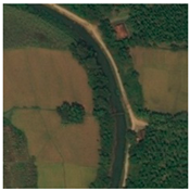 |  |  | 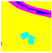 | ||
| FSS |  |  |  |  | ||
| FSS-RSI | 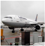 |  | 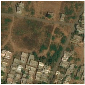 |  | ||
| Dataset | Numbers | Classes | FID |
|---|---|---|---|
| PASCAL-5i | 17,125 | person, bird, dog, cat, cow, chair, dining table, potted plant, sheep, horse, airplane, bicycle, boat, car, bottle, sofa, tv/monitor bus, motorbike, and train | – |
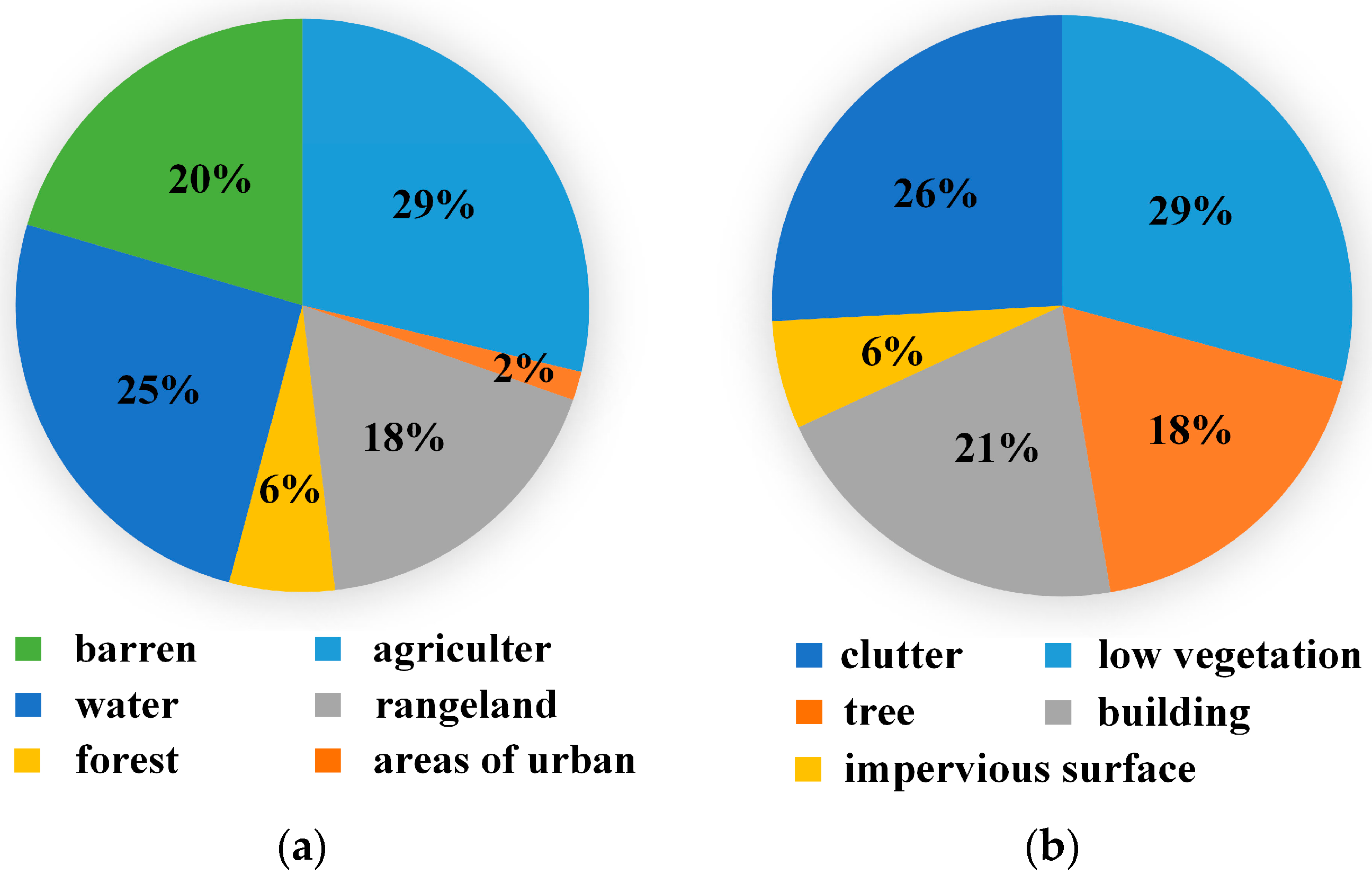
| FSS-RSI-DeepGlobe | 9175 | agricultural, forested, barren, urban, rangeland, and aquatic areas | 186.55 |
| FSS-RSI-Potsdam | 1896 | clutter, tree, low vegetation, building, and impervious surface | 151.86 |
| FSS-RSI-Vaihingen | 308 | tree, low vegetation, building, and impervious surface | 328.08 |
| FSS-RSI-AISD | 5640 | building and road | 194.90 |
| Split-1 | Split-2 | FID |
|---|---|---|
| Fold0 | Fold1 + Fold2 + Fold3 | 79.47 |
| Fold1 | Fold0 + Fold2 + Fold3 | 47.47 |
| Fold2 | Fold0 + Fold1 + Fold3 | 41.45 |
| Fold3 | Fold0 + Fold1 + Fold2 | 61.48 |
| Method | FSS-RSI-DeepGlobe | FSS-RSI-Potsdam | FSS-RSI-Vaihingen | FSS-RSI-AISD | Average | |||||
|---|---|---|---|---|---|---|---|---|---|---|
| 1-Shot | 5-Shot | 1-Shot | 5-Shot | 1-Shot | 5-Shot | 1-Shot | 5-Shot | 1-Shot | 5-Shot | |
| PFENet | 3.97 | 2.42 | 6.26 | 4.84 | 12.58 | 12.29 | 25.03 | 25.18 | 11.96 | 11.18 |
| RPMMs | 10.66 | 13.17 | 6.76 | 7.56 | 16.24 | 16.45 | 25.12 | 23.86 | 14.70 | 15.26 |
| HSNet | 31.78 | 35.38 | 17.94 | 19.31 | 21.78 | 24.16 | 24.47 | 26.41 | 23.99 | 26.32 |
| BAM | 12.23 | 26.65 | 12.53 | 17.37 | 17.19 | 26.98 | 23.35 | 27.41 | 16.33 | 24.60 |
| HDMNet | 16.68 | 17.57 | 11.27 | 23.49 | 21.80 | 25.53 | 21.04 | 25.74 | 17.70 | 23.08 |
| FTNet | 41.37 | 44.57 | 24.68 | 25.58 | 24.75 | 26.44 | 29.51 | 31.14 | 30.08 | 31.93 |
| Method | FSS-IRS-DeepGlobe | FSS-IRS-Potsdam | FSS-IRS-Vaihingen | Average | ||||
|---|---|---|---|---|---|---|---|---|
| 1-Shot | 5-Shot | 1-Shot | 5-Shot | 1-Shot | 5-Shot | 1-Shot | 5-Shot | |
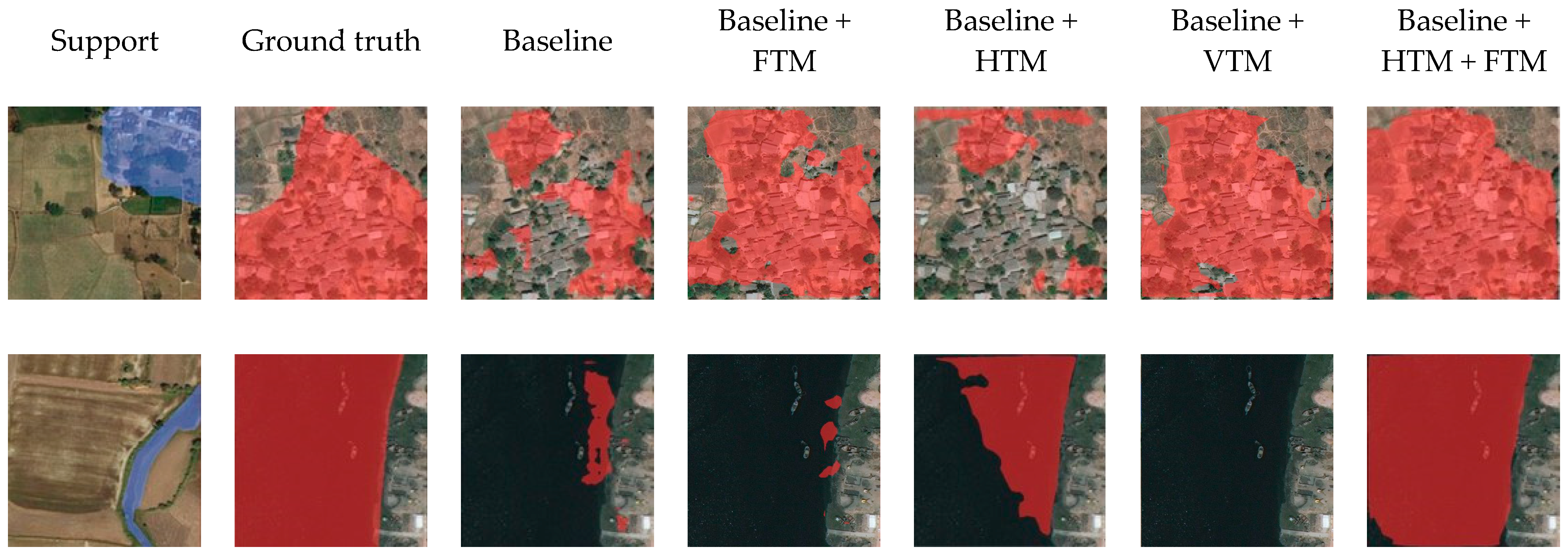
| Baseline | 19.29 | 30.56 | 11.56 | 17.84 | 21.69 | 21.72 | 17.51 | 23.37 |
| Baseline + FTM | 31.62 | 33.80 | 22.57 | 20.86 | 24.73 | 27.61 | 26.31 | 27.42 |
| Baseline + HTM | 38.41 | 43.40 | 23.03 | 23.99 | 23.31 | 25.41 | 28.25 | 30.93 |
| Baseline + VTM | 21.23 | – | 20.27 | – | 23.16 | – | 21.55 | – |
| Baseline + HTM + FTM | 41.37 | 44.57 | 24.68 | 25.58 | 24.75 | 26.44 | 30.27 | 32.20 |
Disclaimer/Publisher’s Note: The statements, opinions and data contained in all publications are solely those of the individual author(s) and contributor(s) and not of MDPI and/or the editor(s). MDPI and/or the editor(s) disclaim responsibility for any injury to people or property resulting from any ideas, methods, instructions or products referred to in the content. |
© 2023 by the authors. Licensee MDPI, Basel, Switzerland. This article is an open access article distributed under the terms and conditions of the Creative Commons Attribution (CC BY) license (https://creativecommons.org/licenses/by/4.0/).
Share and Cite
Sun, Q.; Chao, J.; Lin, W.; Xu, Z.; Chen, W.; He, N. Learn to Few-Shot Segment Remote Sensing Images from Irrelevant Data. Remote Sens. 2023, 15, 4937. https://doi.org/10.3390/rs15204937
Sun Q, Chao J, Lin W, Xu Z, Chen W, He N. Learn to Few-Shot Segment Remote Sensing Images from Irrelevant Data. Remote Sensing. 2023; 15(20):4937. https://doi.org/10.3390/rs15204937
Chicago/Turabian StyleSun, Qingwei, Jiangang Chao, Wanhong Lin, Zhenying Xu, Wei Chen, and Ning He. 2023. "Learn to Few-Shot Segment Remote Sensing Images from Irrelevant Data" Remote Sensing 15, no. 20: 4937. https://doi.org/10.3390/rs15204937
APA StyleSun, Q., Chao, J., Lin, W., Xu, Z., Chen, W., & He, N. (2023). Learn to Few-Shot Segment Remote Sensing Images from Irrelevant Data. Remote Sensing, 15(20), 4937. https://doi.org/10.3390/rs15204937