SDAT-Former++: A Foggy Scene Semantic Segmentation Method with Stronger Domain Adaption Teacher for Remote Sensing Images

Abstract

Semantic segmentation based on optical images can provide comprehensive scene information for intelligent vehicle systems, thus aiding in scene perception and decision making. However, under adverse weather conditions (such as fog), the performance of methods can be compromised due to incomplete observations. Considering the success of domain adaptation in recent years, we believe it is reasonable to transfer knowledge from clear and existing annotated datasets to images with fog. Technically, we follow the main workflow of the previous SDAT-Former method, which incorporates fog and style-factor knowledge into the teacher segmentor to generate better pseudo-labels for guiding the student segmentor, but we identify and address some issues, achieving significant improvements. Firstly, we introduce a consistency loss for learning from multiple source data to better converge the performance of each component. Secondly, we apply positional encoding to the features of fog-invariant adversarial learning, strengthening the model’s ability to handle the details of foggy entities. Furthermore, to address the complexity and noise in the original version, we integrate a simple but effective masked learning technique into a unified, end-to-end training process. Finally, we regularize the knowledge transfer in the original method through re-weighting. We tested our SDAT-Former++ on mainstream benchmarks for semantic segmentation in foggy scenes, demonstrating improvements of 3.3%, 4.8%, and 1.1% (as measured by the mIoU) on the ACDC, Foggy Zurich, and Foggy Driving datasets, respectively, compared to the original version.

1. Introduction

Among the various perception methods, vision-based methods have attracted interest due to their comprehensive, intuitive, and cost-effective advantages [1,2]. In particular, robust semantic segmentation [3,4,5,6,7,8,9,10] based on visual images is important for autonomous driving, as it can save on the huge costs of installing auxiliary sensors (like LiDAR), thereby effectively aiding intelligent vehicles.

However, the segmentation models trained on clear-scene datasets often generalize poorly under adverse weather conditions (such as foggy scenes [11]) due to the degradation of visibility [12]. Meanwhile, the cost of directly producing annotations for foggy images is much higher than for clear ones, which makes it difficult to address the problem of semantic segmentation in foggy scenes (SSFS) using a traditional fully supervised training strategy. At present, the most common way is to transform it into a domain adaptation (DA) problem [13], which uses finely annotated datasets containing clear scenes (such as Cityscapes [14]) as the source domain and foggy scenes as the target domain (with no labels) to transfer the segmentation knowledge by training a DA model. Domain adaptation methods are often based on Generative Adversarial Networks (GANs) [15] and self-training [16]. GAN-based DA methods regard domain differences as noise that needs to be aligned across the input [15,17,18], feature [19], and output spaces [20,21]. Self-training methods [22,23,24,25] use the current model to generate pseudo-labels on the target domain and perform self-guidance. But directly using DA methods makes it challenging to handle large dual-domain differences (such as style differences between cities and visual degradation caused by haze), resulting in poor-quality pseudo-labels. These methods tend to easily generate a large area of classification error at the boundary between fog and objects [11]. Some methods [26,27,28] introduce intermediate domains to reduce the domain gap by collecting or generating a set of images with different degrees of haze or from different time periods using curriculum learning strategies. But they require a large amount of data and are prone to accumulating errors. Recently, introducing a single clear domain as an intermediate domain [29] has gained attention, as this approach only requires collecting clear images from the target city to serve as the intermediate domain. Cycle training or spatial alignment can then be used on this domain to guide the segmentation of target domain images. However, the intermediate domain and target domain information are still treated independently and not fully utilized. In contrast, our method integrates information from various domains through cyclical training, thus achieving the organic integration of information.

Despite the importance of both style gap and fog gap, most methods still focus on only one of them, resulting in little improvement when facing real foggy scenes. This may be due to the different training paradigms. When dealing with the fog gap, adversarial training strategies or explicit fog modeling approaches are often used, whereas excellent, newly developed methods mainly adopt self-training strategies [22,23,25,30] when dealing with the style gap. Simply combining the two strategies can cause interference between sub-modules due to chaotic backward gradients. Recently, the authors of SDAT-Former [1] proposed a strong teacher for foggy road scene semantic segmentation, which differs from previous domain adaptation methods, as it considers both style and fog knowledge, successfully transferring style-invariant knowledge and fog-invariant knowledge to the teacher segmentor [25,31]. This enables the teacher segmentor to have a broader perspective and generate superior pseudo-labels in the target domain, thereby guiding the training of the student segmentor (the main segmentor to be published). Specifically, this method divides the entire training process into several mini-epochs, each consisting of four iterations that perform fog-invariant adversarial learning, intermediate domain style feature learning, information integration, and target domain mask domain adaptation, respectively. This effectively solves the mutual interference between gradients and successfully handles the problem of significant style and fog differences, surpassing the previous year’s state-of-the-art solutions on mainstream foggy scene semantic segmentation benchmarks.

However, SDAT-Former [1] still has many drawbacks. Firstly, the extraction of style features in the intermediate domain is cumbersome and cannot be integrated into an end-to-end training process. SDAT-Former first trains an LSGAN [17] to apply the source domain style to the intermediate domain images, then uses DAFormer [25] to predict the labels of the transformed images. These training steps are performed offline and consume significant computational resources and time. Additionally, when the intermediate domain changes, the corresponding models need to be retrained to generate new data. The style features learned by the GAN-based models may not be comprehensive due to down-sampling operations for calculating discrimination probabilities [17] and artifacts [1]. In this case, the label-based learning approach is prone to introducing noise, which can damage the model. Secondly, in the fog-invariant feature learning step, the original feature dimension is too low, but the actual variations in fog may be subtle, leading to the extracted features not being representative enough. Furthermore, the three components of SDAT-Former contribute equally to the parameters of the teacher segmentor, but in reality, they should be assigned weights or dynamically adjusted. Finally, the performance of each component eventually converges to a stable condition, but the SDAT-Former method does not take this factor into account or adopt appropriate consistency constraints to accelerate convergence.

Based on the above, we propose the improved “SDAT-Former++” which is shown in Figure 1. This new version retains the cyclical training strategy from SDAT-Former [1] but incorporates substantial optimizations. To address the complexity of intermediate domain learning, we introduce a simple but effective strategy using masked autoencoder learning [32,33], which can align the context by predicting masked images. This approach enables the model to better distinguish similar categories such as roads and sidewalks. By directly recovering the masked intermediate domain images, we use a basic backbone to learn the style features of the intermediate domain in a complete and artifact-free manner. Moreover, the knowledge is directly saved in the model’s parameters, thus facilitating an end-to-end training process without the need for extra offline operations. Additionally, the model can start training directly when the intermediate domain changes, achieving a complete separation between the model and the data. To tackle the problem of low feature dimensions and inadequate representations in fog-invariant learning, we introduce positional encoding [34,35] to separate more high-dimensional details, making the fog discriminator more sensitive and compelling the fog-invariant feature extractor to be robust. To address the issue of evenly distributed knowledge transfer, we introduce weight perturbations based on a random distribution for regularization.

Compared to the original SDAT-Former publication, this paper provides more comprehensive experimental results and technical details. In addition to the existing ACDC [36] and Foggy Zurich [27] datasets, a more challenging dataset, Foggy Driving Dense [37], is also included. We also conduct extensive ablation experiments and provide favorable entropy analysis evidence.

The contributions of this work can be summarized as follows:

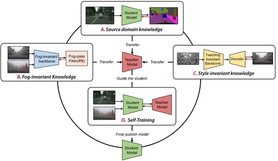
• To the best of our knowledge, this work is the first to propose an end-to-end cyclical training domain adaptation semantic segmentation method that considers both style-invariant and fog-invariant features.
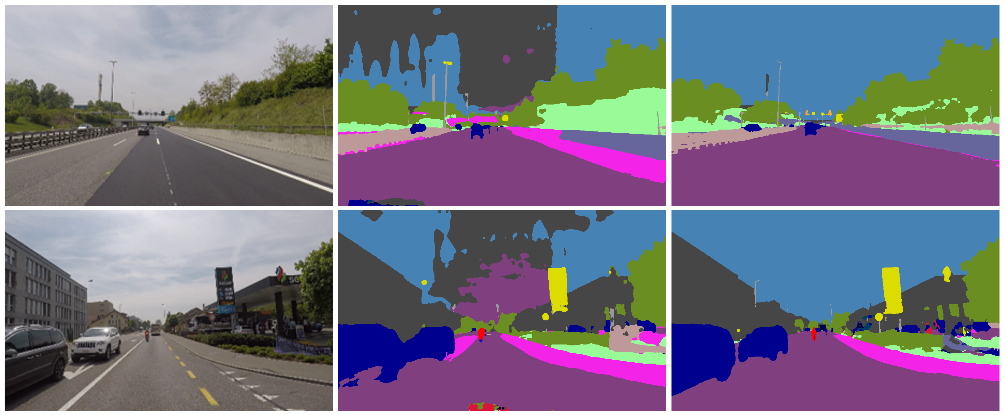
• Our method proves the importance of masked learning and feature enhancement in foggy road scene segmentation and demonstrates their mechanisms through visualizations.
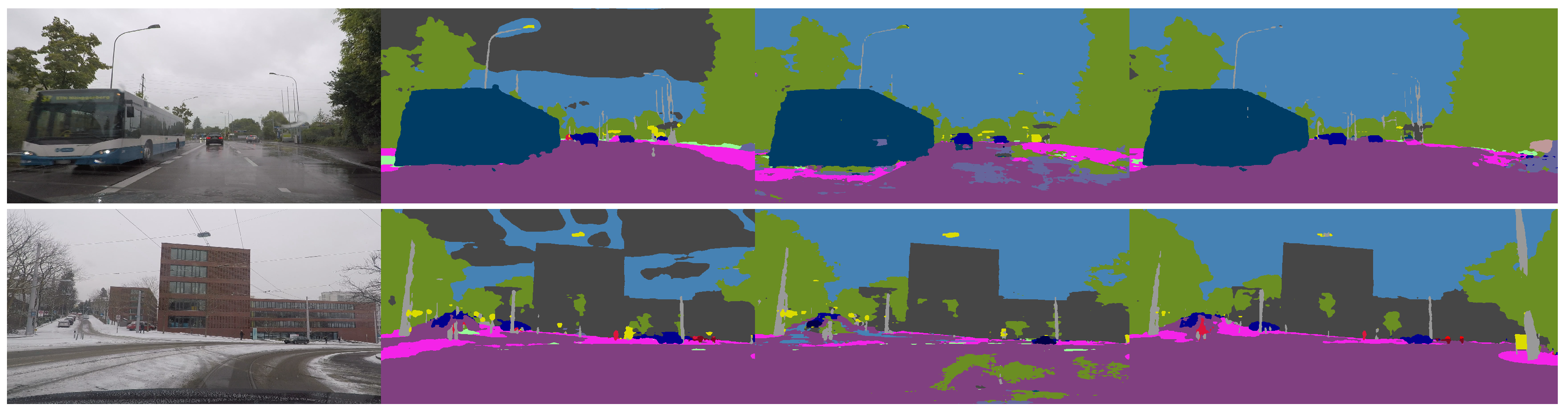
• Our method significantly outperforms SDAT-Former on mainstream benchmark datasets for foggy road scene segmentation and exhibits strong generalization in rainy and snowy scenes. Compared to the original method, SDAT-Former++ pays more attention to the more important categories in road scenes and is more suitable for applications in intelligent vehicles. We test our SDAT-Former++ method on mainstream benchmarks for semantic segmentation in foggy scenes and demonstrate improvements of 3.3%, 4.8%, and 1.1% (as measured by the mIoU) on the ACDC, Foggy Zurich, and Foggy Driving datasets, respectively, compared to the original method.

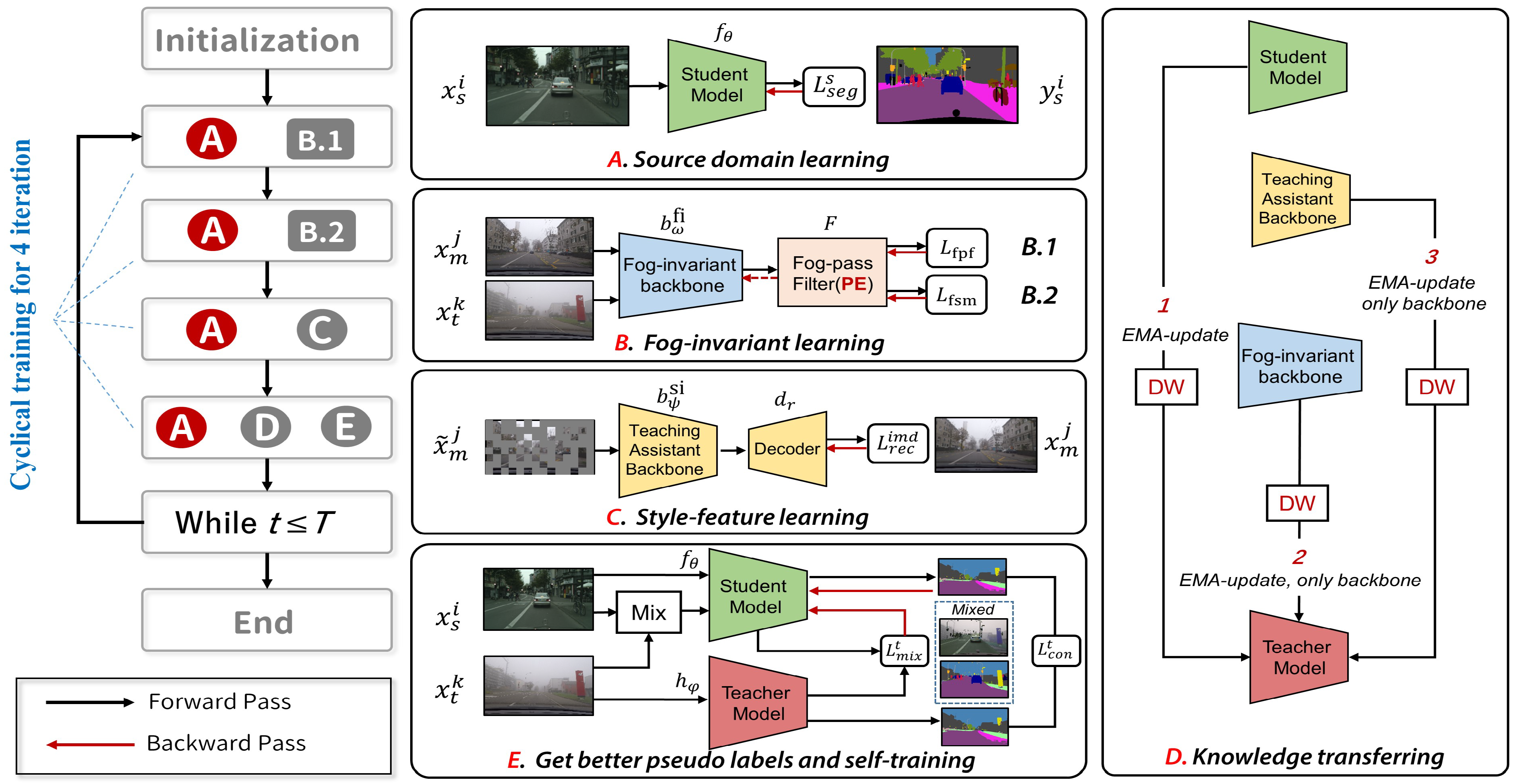
2. Method

2.1. Overview

Suppose there are $N_s$ labeled images ${\left\{\left(x_s^i,y_s^i\right)\right\}}_{i=1}^{N_s}$ from the clear source domain s, where $y_s^i$ is the pixel-level segmentation label for $x_s^i$, and $N_t$ unlabeled images ${\left\{x_t^k\right\}}_{k=1}^{N_t}$ from the target foggy domain t. Our goal is to transfer segmentation knowledge from the clear source domain s to the foggy target domain t using our proposed SDAT-Former++ method. Motivated by the success of DAFormer [25], we use a similar framework including a “student” segmentor and a “teacher” segmentor to train in a self-training manner. However, since the images in domain s and domain t were taken in different cities and under different weather conditions, they exhibit a large domain gap caused by two factors, i.e., the style factor and the fog factor, which poses a challenge to this method. Therefore, we introduce an intermediate domain m with $N_m$ unlabeled images ${\left\{\left(x_m^j\right)\right\}}_{j=1}^{N_m}$. This domain shares similar fog influence (no fog) to the source domain and similar style variation to the target domain (imaged in the same city). We also call these images the “reference images” $I^{\mathrm{ref}}$ of the foggy images $I^{\mathrm{fog}}$. Thus, our main goal is to cumulatively transfer four kinds of knowledge to the “teacher” segmentor to generate more robust pseudo-labels of t, thereby empowering the “student” segmentor to complete the segmentation tasks: (a) segmenting the knowledge from s, (b) segmenting the style knowledge from m, (c) segmenting the knowledge from t, and (d) identifying and removing fog. Among these, (c) and (d) focus on overcoming the “fog gap” between s and t, whereas (b) focuses on the “style gap”. Figure 2 depicts the framework of our proposed method.

Concretely, we reorganize the training workflow cyclically, where every four iterations constitute a “mini-epoch”. The segmentation knowledge from s can be learned from labels ${\left\{\left(y_s^i\right)\right\}}_{i=1}^{N_s}$ in a supervised way (Figure 2A), and we train it throughout the process. In the first iteration of a mini-epoch, a fog-pass filter [38] is trained for discriminating fog factors from the clear source domain m and foggy target domain t (Figure 2B.1). Here, we use positional encoding (PE) [34,35] to enhance the features and capture more high-frequency information. In the second iteration, the segmentor backbone is trained to generate features that fool the fog-pass filter (Figure 2B.2). These two iterations aim to train a robust extractor for fog-invariant features in an adversarial manner. For the third iteration, we abandon the complex operation mode in the original version of the method [1] and use a feature extractor with a decoder to recover the masked images ${\left\{\left({\tilde{x}}_m^j\right)\right\}}_{j=1}^{N_m}$ from the intermediate domain and extract style features. In the last iteration, the parameters stored in the teacher segmentor can be updated by the “student” segmentor (containing knowledge from s), the “teaching-assistant” backbone (containing style knowledge from m), and the fog-invariant backbone (containing fog-invariant knowledge) in an exponential moving average (EMA) [31] way with dynamic weight (DW) (Figure 2D. Then, the self-training process is performed on the target foggy domain t. Thus, the “teacher” can be “strong” enough to handle the domain gap and guide the student (main) segmentor.

2.2. Sub-Modules

The main workflow includes 6 sub-modules: (a) “student” segmentor $f_{\theta }$ (can be published as the final segmentor), (b) “teaching assistant” backbone $b_{\psi }^{\mathrm{si}}$ (learns the style knowledge), (c) decoder $d_r$ for reconstruction, (d) “teacher” segmentor $h_{\phi }$, (learns knowledge from the target domain), (e) fog-invariant backbone $b_{\omega }^{\mathrm{fi}}$, and (f) fog-pass filter $\mathcal{F}$ (learns to recognize fog factors).

All the segmentors contain a backbone and decoder head. The backbone follows the design of Mix Transformers (MiT) [39] to produce multi-level feature maps, whereas the decoder head follows ASPP [40] to predict segmentation maps. The fog-invariant backbone $b_{\omega }^{\mathrm{fi}}$ shares the same architecture as MiT for subsequent knowledge transfer. The fog-pass filter $\mathcal{F}$ follows the design in FIFO [38]. The detailed architectures are described later.

2.3. Supervised Training on Source Domain

Denote H and W as the height and width of the input image size and C as the number of object categories. First, we can use $f_{\theta }$ to learn the segmentation knowledge from the labeled source domain ${\left\{\left(x_s^i,y_s^i\right)\right\}}_{i=1}^{N_s}$ using a categorical cross-entropy loss function:

$${\mathcal{L}}_s^i=-\sum _{p=1}^{H\times \mathrm{W}}\sum _{c=1}^C{y}_s^{(i,p,c)}log{f}_{\theta }{\left(x_s^i\right)}^{(p,c)}$$

(1)

2.4. Masked Learning on the Intermediate Domain

In the original version of SDAT-Former [1], an LSGAN [17] is used to transfer styles between the source domain and the intermediate domain. Then, the source styles are applied to the later images to narrow the domain gap. Next, a DAFormer [25] model is used to predict the transformed images ${\left\{\left({\tilde{x}}_m^j\right)\right\}}_{j=1}^{N_m}$ and generate pseudo-labels, which have the same spatial layout as the original images ${\left\{\left(x_m^j\right)\right\}}_{j=1}^{N_m}$. This method adds two offline training steps and results in a significant loss in the resolution and details of the predicted values, even leading to artifacts. Training based on such pseudo-labels inevitably introduces noise. Moreover, when changing the intermediate domain, we have to reconfigure two pre-trained networks, influencing the deployment.

Since learning based on intermediate domain data aims to capture style features, pseudo-labels may not be necessary. In this section, we introduce a more concise method to model masked images. Specifically, we employ a uniform distribution to randomly sample a mask:

$$\begin{array}{cc}{M}_{{}_{nb+1:(n+1)b}^{mb+1:(m+1)b}}=\left[v\ge r\right]& \begin{array}{cc}\mathrm{with}& v\sim U(0,1)\end{array}\end{array}$$

(2)

where $[\ast ]$ is the Iverson bracket, b is the patch size, r is the mask ratio, and $m\in \left[0..W/b-1\right]$ and $n\in \left[0..H/b-1\right]$ are the patch indices. Thus, we obtain the masked intermediate image ${\tilde{x}}_m^j$ through element-wise multiplication of the mask and image:

$${\tilde{x}}_m^j=M\odot x_m^j$$

(3)

Then, we try to use encoder $b_{\psi }^{\mathrm{si}}$ and decoder $d_r$ to recover the original image:

$$x_m^{j,rec}=b_{\psi }^{\mathrm{si}}\left(d_r\left({\tilde{x}}_m^j\right)\right)$$

(4)

We force the model to adopt the L1 loss function to recover the original image information. As a result, the feature extraction network obtains more realistic and context-aware style features, which are difficult to achieve through label-based approaches and do not lead to any resolution loss or noise:

$${\mathcal{L}}_m^{rec}=|x_m^{j,rec}-x_m^j|$$

(5)

The knowledge from the intermediate domain can be stored in the parameters of $b_{\psi }^{\mathrm{si}}$, which can be passed to the “teacher” segmentor rather than being directly transferred to the final segmentor. This part is described in Section 2.7.

2.5. Fog-Invariant Feature Learning

Here, we focus on overcoming the fog gap between the intermediate domain and the target domain. Since Section 2.4 described the learning of cross-style knowledge, now, we only need to process the fog factor. That is, the final segmentor should output the fog-invariant features from the pair of foggy and non-foggy images. To achieve this, we design a fog-invariant feature extractor $b_{\omega }^{\mathrm{fi}}$ and a fog-pass filter $\mathcal{F}$ based on the architecture of FIFO [38].

2.5.1. Training the Fog-Pass Filter

Given a pair of images $(I^a,I^b)$ from the mini-batch, $b_{\omega }^{\mathrm{fi}}$ can output L layer features of each image. We follow FIFO [38] to calculate these features’ Gram matrix to capture a holistic fog representation denoted as ${\left\{({\mathbf{u}}^{a,l},{\mathbf{u}}^{\mathrm{b},\mathrm{l}})\right\}}_{l=1}^L$. Denote ${\mathcal{F}}^l$ as the fog-pass filter attached to the $l^{th}$ layer feature. The fog factors of these two images can be computed by ${\mathbf{f}}^{\mathrm{a},\mathrm{l}}={\mathcal{F}}^l\left({\mathbf{u}}^{\mathrm{a},\mathrm{l}}\right)$ and ${\mathbf{f}}^{\mathrm{b},\mathrm{l}}={\mathcal{F}}^l\left({\mathbf{u}}^{\mathrm{b},\mathrm{l}}\right)$, respectively.

To enhance the representation of the fog factors, we follow previous works [34,35,41] and adopt a sinusoidal positional encoding scheme to capture the high-frequency details:

$$\psi \left(\mathbf{f}\right)=(sin\left({\omega }_1\mathbf{f}\right),cos\left({\omega }_1\mathbf{f}\right),...,sin\left({\omega }_n\mathbf{f}\right),cos\left({\omega }_n\mathbf{f}\right))$$

(6)

where the frequencies ${\omega }_1,{\omega }_2,...{\omega }_n$ are learnable during training and n is the positional encoding dimension. The role of the fog-pass filter is to inform the fog-invariant backbone $b_{\omega }^{\mathrm{fi}}$ about how $I^a$ and $I^b$ are different in terms of fog conditions through $\psi \left({\mathbf{f}}^{\mathrm{a},\mathrm{l}}\right)$ and $\psi \left({\mathbf{f}}^{\mathrm{b},\mathrm{l}}\right)$. For this purpose, the fog-pass filter learns a space of fog factors, where those of the same fog domain are grouped closely together and those of different domains are far apart. The loss function for ${\mathcal{F}}^l$ is designed as follows:

$$\begin{array}{c}\hfill {\mathcal{L}}_{{\mathcal{F}}^l}={\displaystyle \sum _{(a,b)}}(1-\mathsf{\Pi }(a,b)){\left[m-d(\psi \left({\mathbf{f}}^{\mathrm{a},\mathrm{l}}\right),\psi \left({\mathbf{f}}^{\mathrm{b},\mathrm{l}}\right))\right]}^2\\ \hfill +\mathsf{\Pi }(a,b){\left[d(\psi \left({\mathbf{f}}^{\mathrm{a},\mathrm{l}}\right),\psi \left({\mathbf{f}}^{\mathrm{b},\mathrm{l}}\right))-m\right]}^2\end{array}$$

(7)

where $d\left(\right)$ is the cosine distance, m is the margin, and $\mathsf{\Pi }(a,b)$ denotes the indicator function that returns 1 if $I^a$ and $I^b$ are of the same fog domain and 0 otherwise.

2.5.2. Fog Factor Matching Loss

In contrast to the function of the fog-pass filter, which attempts to separate the fog factors of different fog domains, the fog-invariant backbone $b_{\omega }^{\mathrm{fi}}$ learns to close the distance between the fog factors. To this end, the second loss matches the two fog factors given by frozen fog-pass filters:

$${\mathcal{L}}_{fsm}^l(\psi \left({\mathbf{f}}^{a,l}\right),\psi \left({\mathbf{f}}^{\mathrm{b},l}\right))=\frac{1}{4d_l^2{n}_l^2}\sum _{i=1}^{d_l}{(\psi \left({\mathbf{f}}_i^{a,l}\right)-\psi \left({\mathbf{f}}_i^{b,l}\right))}^2$$

(8)

where $d_l$ and $n_l$ denote the dimensions of their fog factors and the spatial size of the $l^{th}$ feature map, respectively. The knowledge from fog-invariant training can be also stored in the parameters in $b_{\omega }^{\mathrm{fi}}$ and can be passed to the “teacher” segmentor, as described in Section 2.7.

2.6. Self-Training on the Target Domain and Consistency Learning

We use a teacher segmentor $h_{\phi }$ to directly address the two gaps (style + fog) between the source domain and the target domain to obtain better domain adaptation performance. Specifically, $h_{\phi }$ can first produce pseudo-labels for the foggy target domain data

$${\tilde{y}}_t^{(k,p,c)}=\left[c=arg{max}_{c^{\prime }}{h}_{\phi }{\left(x_t^k\right)}^{(p,c^{\prime })}\right]$$

(9)

Additionally, a quality (confidence) estimation is produced for the pseudo-labels. Here, we use the ratio of pixels exceeding a threshold $\tau$ of the maximum softmax probability

$$q_t^k=\frac{{\sum }_{p=1}^{H\times W}\left[{max}_{c^{\prime }}{h}_{\phi }{\left(x_t^k\right)}^{(p,c^{\prime })}\ge \tau \right]}{H\times W}$$

(10)

The pseudo-labels and their quality estimates are used to additionally train the segmentor $h_{\phi }$ on the target domain

$${\mathcal{L}}_t^k=-\sum _{p=1}^{H\times \mathrm{W}}\sum _{c=1}^C{q}_t^k{\tilde{y}}_t^{(k,p,c)}log{h}_{\phi }{\left(x_t^k\right)}^{(p,c)}$$

(11)

The self-training process can be more efficient if the segmentor is trained on augmented data [42]. In this work, we follow DACS [23] and employ color jitter, Gaussian blur, and ClassMix [43] for data augmentation to learn more domain features. To accelerate the training, we introduce a consistency learning strategy between teacher $h_{\phi }$ and student $f_{\theta }$. Specifically, for one specific sample x, we use the Kullback–Leibler divergence as a consistency loss, forcing convergence between the teacher and student

$${\mathcal{L}}_{con}\left(x\right)=\sum _i\mathrm{KLdiv}(f_{\theta }\left(x\right),h_{\phi }\left(x\right))$$

(12)

2.7. Cyclical Training with Knowledge Transferring

The above steps facilitate domain adaptation learning from different levels, but they need to be organically combined. If we include so many backward processes in a single iteration, the gradient propagation could be easily confused and the sub-modules could face potential interface issues Thus, we use cyclical training and build a “strong teacher” to merge the above-mentioned knowledge. We divide every four iterations into a “mini-epoch”. Considering that fog-invariant feature learning works adversarially, we allocate the $1st$ and $2nd$ iterations to train the fog-pass filter $\mathcal{F}$ and fog-invariant backbone $b_{\omega }^{\mathrm{fi}}$ successively. The $3rd$ iteration is allocated to intermediate domain learning using the teaching-assistant segmentor $g_{\psi }$. For the $4th$ iteration, since the intermediate feature extractor $b_{\psi }^{\mathrm{si}}$ does not need to complete segmentation, we remove the pre-updating used in [1] to prevent interface issues. All the knowledge can be transferred to the teacher segmentor through an optimized three-step exponentially moving average (EMA [31]) update (Figure 2D):

$$\begin{array}{c}{h}_{\phi }^{t+1}={\alpha }_1{h}_{\phi }^t+(1-{\alpha }_1)b_{\omega }^{\mathrm{fi}|\mathrm{t}}\\ \\ h_{\phi }^{t+2}={\alpha }_2{h}_{\phi }^{t+1}+(1-{\alpha }_2)f_{\theta }^t\\ \\ h_{\phi }^{t+3}={\alpha }_3{h}_{\phi }^{t+2}+(1-{\alpha }_3)b_{\psi }^{\mathrm{si}|\mathrm{t}}\\ \end{array}$$

(13)

where $\begin{array}{cc}{\alpha }_i=\alpha +{\delta }_i& {\delta }_i\sim N(0,V)\end{array}$, i.e., the parameters are perturbed by a normal distribution and thus the knowledge can be regularized. Then, we conduct self-training on the target domain, as described in Section 2.6. In our proposed method, we use EMA [31] to update the model parameters because it can transmit domain knowledge while protecting the segmentor from the noise in the pseudo-labels [44]. Thus, the teacher segmentor can be powerful enough to guide the student segmentor in the domain adaptation training. In the ablation study, we discuss EMA updating in detail.

3. Results

3.1. The Network Parameters

Our implementation was based on the mmsegmentation framework [45] and PyTorch [46]. The MiT-b5 backbone (used in $f_{\theta }$, $h_{\phi }$, $g_{\psi }$, and $b_{\omega }^{\mathrm{fi}}$) produced a feature pyramid with channels of 64, 128, 320, and 512. The ASPP decoder used $n_{ch}=256$ and dilation rates of 1, 6, 12, and 18. All encoders were pre-trained on the ImageNet-1k [47] dataset. The fog-pass filters $\mathcal{F}$ were composed of a fully connected layer and LeakyReLU layer to convert the Gram matrix of the feature maps into fog vectors.

3.2. Implementation Details

The main workflow was trained by AdamW [48], the learning rate was $6\times {10}^{-5}$ with a weight-decay of 0.01, and linear learning rate warm-up followed the “poly” strategy after 1.5k iterations. All the input images and labels were cropped to $512\times 512$, and the maximum number of training iterations was 40k. Following DACS [23], we used the same data augmentation parameters and set $\alpha =0.99$, $\tau =0.968$, and the perturbation variance $V=0.1$. We set the weight of the source domain supervised learning loss (Equation (1)) to 1 and the weight of the intermediate domain style feature learning loss (Equation (5)) to 0.5. Following FIFO [38], we set the loss weights for both the fog-pass-filter loss (Equation (7)) and the fog factor matching loss (Equation (8)) to 0.001, with $m=0.1$. We set the weight of the consistency learning loss (Equation (12)) to 0.1 to avoid learning errors from the teacher network. The weight of the loss function in the target domain had already been determined based on confidence and did not need to be set manually. The dimension n for positional encoding was set to 512. All the experiments were conducted on a single Tesla-v100 GPU with a memory of 32 GB and equipped with CUDA 10.2.

3.3. Datasets

Cityscapes [14] is a real-world dataset composed of street scenes captured in 50 different cities. The data split includes 2975 training images and 500 validation images with pixel-level labels. The Cityscapes dataset is the source domain and shares the same class set with all the datasets mentioned in this paper.

ACDC [36] contains four categories of adverse conditions (fog, snow, rain, and nighttime) with pixel-level annotations. Each category contains 1000 images and is split into a train set, validation set, and test set at a ratio of about 4:1:5. The annotations of the test set were withheld for online testing. We mainly used the foggy images. Moreover, the ACDC dataset also provides clear reference images of each foggy image, which can be used as the intermediate domain.

Foggy Zurich [11] contains 3808 real foggy road views from the city of Zurich and its suburbs. It is split into two categories of fog density—light and medium—consisting of 1552 and 1498 images, respectively. It has a test set, Foggy Zurich-test, which includes 40 images with labels that are compatible with those of Cityscapes.

Foggy Driving [11] contains 101 real-world foggy images collected from the Internet with different sizes and fog densities, including a challenging subset of 21 images with “dense fog” (referred to as Foggy Driving Dense) [37]. The dataset can only be used for evaluation.

The comparison results are shown in

Table 1. Performance comparison I. Experiments were conducted on the ACDC [36] and Foggy Zurich-test (FZ) [27] dataset, measuring the mean intersection over union (mIoU) (%) across all 19 classes following the Cityscapes [14] benchmark.

Experiment	Method	Backbone	ACDC	FZ	Experiment	Method	Backbone	ACDC	FZ
Backbone	-	DeepLabv2 [49]	33.5	25.9	DA-based	LSGAN [17]	DeepLabv2	29.3	24.4
	-	RefineNet [50]	46.4	34.6		Multi-task [51]	DeepLabv2	35.4	28.2
	-	MPCNet [4]	45.9	39.4		AdaptSegNet [20]	DeepLabv2	31.8	26.1
	-	SegFormer [39]	47.3	37.7		ADVENT [21]	DeepLabv2	32.9	24.5
Dehazing	DCPDN [52]	DeepLabv2	33.4	28.7		CLAN [22]	DeepLabv2	38.9	28.3
	MSCNN [53]	RefineNet	38.5	34.4		BDL [30]	DeepLabv2	37.7	30.2
	DCP [54]	RefineNet	34.7	31.2		FDA [55]	DeepLabv2	39.5	22.2
	Non-local [56]	RefineNet	31.9	27.6		DISE [19]	DeepLabv2	42.3	40.7
	SGLC [57]	RefineNet	39.2	34.5		ProDA [24]	DeepLabv2	38.4	37.8
Synthetic	SFSU [11]	RefineNet	45.6	35.7		DACS [23]	DeepLabv2	41.3	28.7
	CMAda [27]	RefineNet	51.1	46.8		DAFormer [25]	SegFormer	48.9	44.4
	FIFO [38]	RefineNet	54.1	48.4		CuDA-Net [26]	DeepLabv2	55.6	49.1
SDAT	SDAT-Former [1]	SegFormer	56.0	49.0	Ours	SDAT-Former++	SegFormer	59.3	53.8

and

Table 2. Performance comparison II. Experiments were conducted on the Foggy Driving [11] and Foggy Driving Dense [37] datasets, measuring the mean intersection over union (mIoU) (%) across all classes.

Experiment	Method	Backbone	FD	FDD
Backbone	-	DeepLabv2 [49]	26.3	17.6
	-	RefineNet [50]	34.6	35.8
	-	SegFormer [39]	36.2	37.4
Synthetic	CMAda3 [27]	RefineNet	49.8	43.0
	FIFO [38]	RefineNet	50.7	48.9
DA-based	AdaptSegNet [20]	DeepLabv2	29.7	15.8
	ADVENT [21]	DeepLabv2	46.9	41.7
	FDA [55]	DeepLabv2	21.8	29.8
	DAFormer [25]	SegFormer	47.3	39.6
	CuDA-Net [26]	DeepLabv2	53.5	48.2
Ours	SDAT-Former [1]	SegFormer	54.3	50.8
	SDAT-Former++	SegFormer	55.4	51.2

.

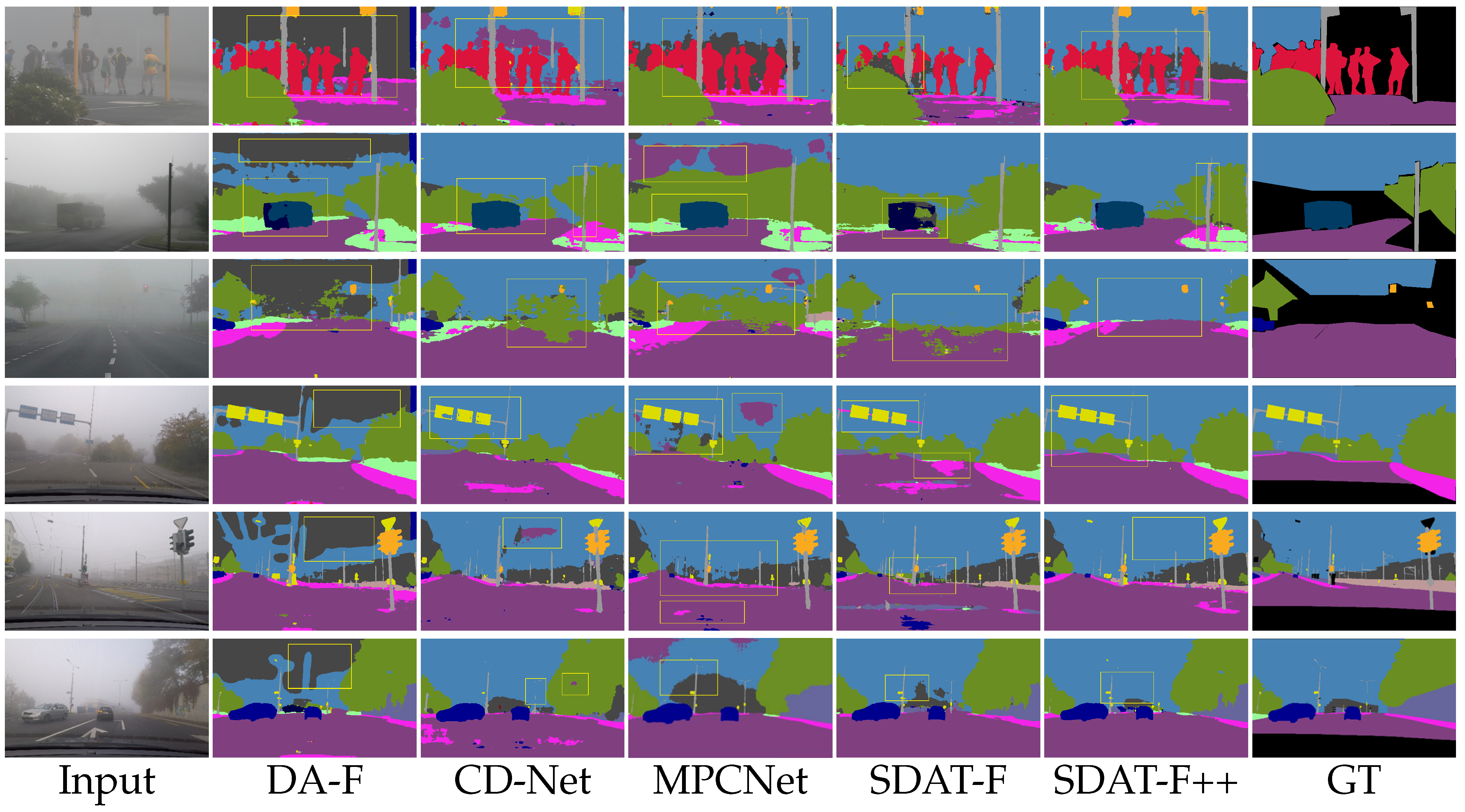
3.4. Performance Comparison

We compared our method to several categories of methods, including:

• Backbones: RefineNet [50], Deeplabv2 [49], MPCNet [4], and SegFormer [39].
• Dehazing methods: MSCNN [53], DCP [54], SGLC [57], DCPDN [52], and non-local [56].
• DA-based methods: LSGAN [17], AdaptSegNet [20], Multi-Task [51], ADVENT [21], CLAN [22], BDL [30], FDA [55], DISE [19], ProDA [24], DACS [23], DAFormer [25], and CuDA-Net [26].
• Synthetic methods: SFSU [11], CMAda [27], and FIFO [38]

The configuration of each type of method was as follows. We trained the backbone methods on the Cityscapes dataset with labels and tested them on the ACDC and Foggy Zurich datasets to evaluate their performance across the domains. We set the source domain for the DA-based methods as clear Cityscapes, representing the s domain in our method. We used the fog images from ACDC and Foggy Zurich (with medium-level fog) as the target domain data. For the intermediate domain m, we combined the ACDC fog reference set (1000 images) with a manual selection of 600 clear images from the Foggy Zurich dataset (light-level fog). For the synthetic methods, the paradigm was to fine-tune the segmentation model pre-trained on clear weather images from Cityscapes. This fine-tuning used synthetic foggy images, such as those from Foggy Cityscapes DBF [11], along with labels corresponding to their clear weather images. We first used the dehazing methods to dehaze the foggy images and then used the corresponding backbone segmentor for predictions.

We compared our method to other outstanding works on the relatively easy ACDC-test [36] and Foggy Zurich-test [27] datasets. Table 1 shows the results, and the results from the ACDC dataset can be found on the https://acdc.vision.ee.ethz.ch/benchmarks#semanticSegmentation (accessed on 11 February 2023). ACDC-fog benchmark website (with our method named “SDAT-Former++”). Our method significantly outperformed the baseline algorithm DAFormer [25], yielding 10.4% and 9.4% higher mIoU values on the two datasets, respectively. Our method also outperformed the recently proposed MPCNet (in RS 2023 [4]) and SGLC (in CVPR23) [57], thus demonstrating the necessity of developing semantic segmentation methods for foggy scenarios. Compared to the original SDAT-Former [1], our method achieved improvements of 3.3% and 3.4%. This indicates that our method is robust without any special operations or removal of fog. Since the ground truths from the ACDC-test dataset were withheld, we used the Foggy Zurich-test [27] and Foggy Driving Dense datasets for qualitative comparison. The upper three rows in Figure 3 show the results on the challenging Foggy Driving Dense dataset [11], and the bottom three rows correspond to Foggy Zurich images output by DAFormer [25] (our baseline), CuDA-Net [26], MPCNet [4], SDAT-Former [1], and SDAT-Former++. Due to DAFormer’s inability to handle style differences in intermediate domains, it failed to handle the sky in foggy conditions. CuDA-Net removed these artifacts but made mistakes in identifying objects occluded by fog (as shown by the yellow box). MPCNet tended to classify fog as buildings or fences. In contrast, our method was highly accurate in segmenting details and handling fog.

Then, we tested our method on the Foggy Driving (FD) [11] and the more challenging Foggy Driving Dense (FDD) [37] datasets. Many methods lost competitiveness or were completely ineffective on these datasets, so only a subset of methods was chosen for comparison. In Table 2, it can be seen that our method achieved improvements of 8.1% and 12.6% in terms of the mIoU over the baseline algorithm DAFormer [25] on FD and FDD, respectively. Our method also outperformed CuDA-Net (with improvements of 1.9% and 3.0%) and FIFO (with improvements of 4.7% and 2.4%). In Figure 3, it can be seen that our method better preserved the segmentation of small objects in the images, for example, the “pole” in the second row, the traffic lights in the third row, and the road signs in the fourth row. This indicates that our method can effectively distinguish small objects while removing the effects of fog, which is crucial for the stability of segmentation.

4. Discussion

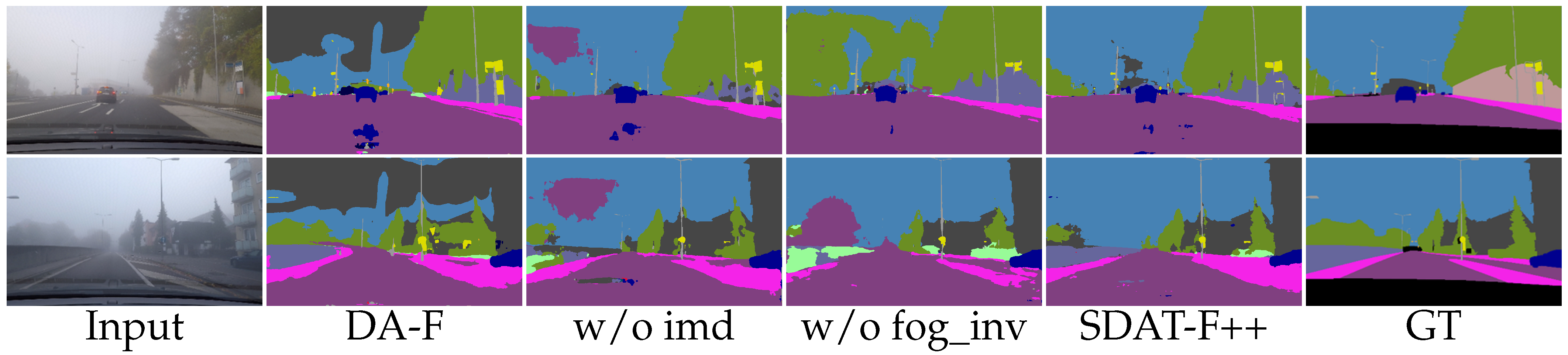
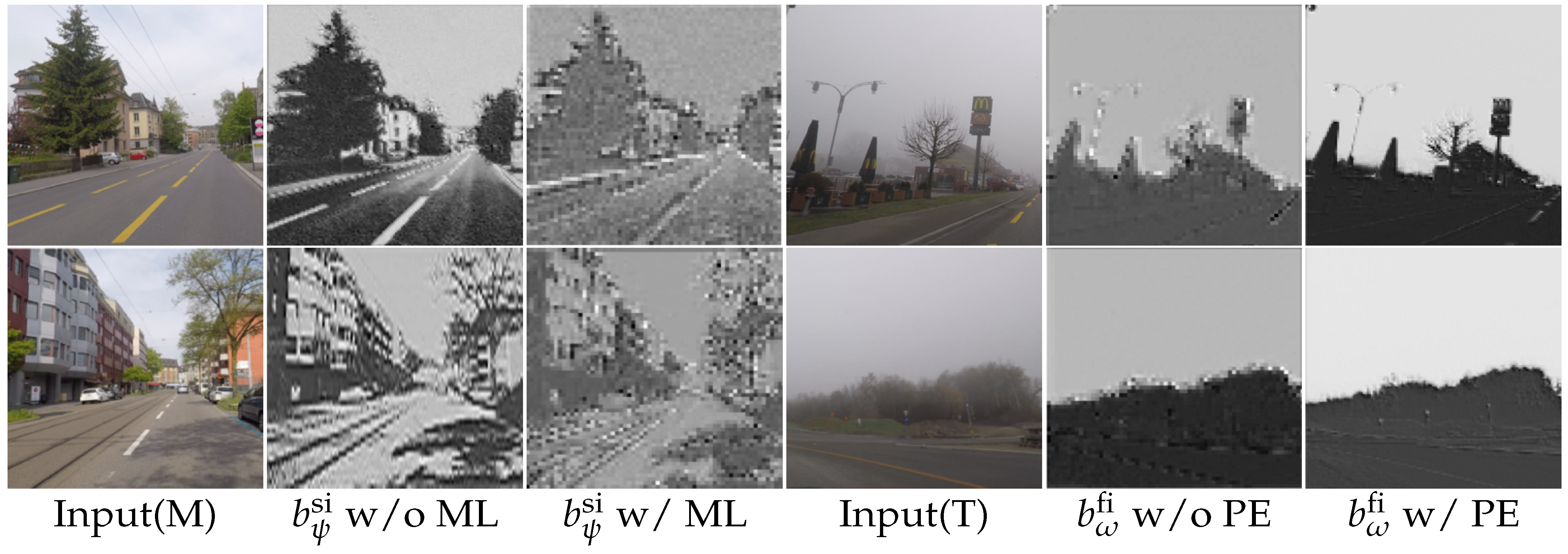
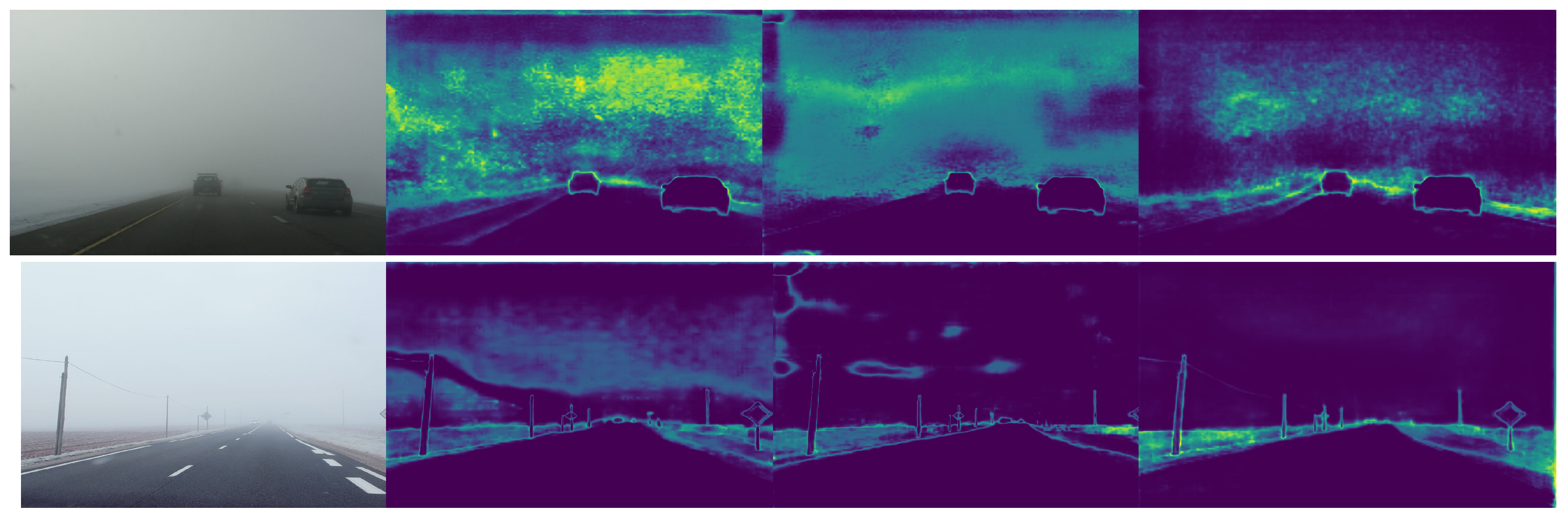
4.1. Effectiveness of Fog-Invariant Feature Learning

In

Table 3. Ablation study. We conducted an ablation study on the ACDC-test dataset, measuring the mIoU (%) across all classes.

Experiment					mIoU	Gain
Initialization	DAFormer				48.92	+0.00
	Cyclical(w/o DW ${}^1$)	imd(ls+da) ${}^2$	fog_inv ${}^3$(w/o PE ${}^4$)		mIoU	Gain
SDAT-F [1]					10.23	−38.69
	✓				49.88	+0.96
		✓			50.52	+1.60
	✓	✓			51.61	+2.69
	✓		✓		53.84	+4.92
	✓	✓	✓		55.98	+7.06
	Cyclical(w/ DW)	imd(masked)	con_learn ${}^5$	fog_inv(w/ PE)	mIoU	Gain
SDAT-F++	✓				50.34	+1.42
		✓			52.63	+3.71
			✓		51.33	+2.41
	✓	✓			56.19	+7.27
	✓		✓	✓	58.42	+9.50
	✓	✓	✓	✓	59.28	+10.36

¹ Indicates dynamic weight allocation. ² Indicates use of LSGAN [17] and DAFormer [25] to obtain pseudo-labels. ³ Note that cyclical training is necessary for fog-invariant learning; we did not experiment with fog-invariant learning alone. ⁴ Indicates positional encoding. ⁵ Consistency learning.

, it can be seen that the non-modified DAFormer, which is also the baseline of the original SDAT-Former, only yielded an mIoU of 48.92% on ACDC. Since we used adversarial training to acquire fog-invariant features, cyclical training was necessary to avoid gradient interference. This shows that the segmentor achieved an mIoU gain of +4.92% after the addition of this component, which was the most significant contribution to the performance improvement.

As depicted in the qualitative results in Figure 4, without fog-invariant learning, the segmentor exhibited prediction drift in foggy conditions, such as misidentifying the sky as vegetation and road, which is consistent with the reports in FIFO [38].

For SDAT-Former++, a 9.50% improvement in the mIoU was achieved after performing fog-invariant feature learning, and the incorporation of positional encoding resulted in a further performance improvement (4.58% higher), indicating that positional encoding effectively enhanced the depiction of fog-related details in images. Figure 5 demonstrates this in two aspects: (1) capturing motion blur and (2) improving the identification of obscured objects within the fog. As shown in the first row, the original SDAT-Former exhibited incomplete segmentation of nearby objects, whereas SDAT-Former++ effectively overcame motion blur, thereby contributing to safer vehicle behavior. In the second row, SDAT-Former failed to detect a tree hidden in the dense fog, whereas the new version with positional encoding accurately captured this obscured element.

4.2. Effectiveness of Style-Invariant Features Learning

In Figure 4, without the help of the intermediate domain, the segmentor misjudged the sky and some ground categories, even with the fog-invariant module. Interestingly, the original DAFormer identified the sky as buildings, but after adding the intermediate domain information, this prediction became vegetation and road. This also illustrates the influence of style information implicitly.

The knowledge from the intermediate domain was mainly used to help the segmentor address the style gap. For SDAT-Former, the segmentor achieved an mIoU gain of +1.60% by learning on the intermediate domain. For SDAT-Former++, this gain was 3.71%. As mentioned before, pseudo-label learning based on style transformations introduces noise. Figure 6 shows some bad pseudo-labels with artifacts and incomplete segmentation of entities. This can inevitably affect training. After SDAT-Former++ adopted mask learning, these problems were avoided.

4.3. Effectiveness of Cyclical Training

The main purpose of cyclical training was to integrate different training paradigms. It did not significantly improve the performance of the segmentor, but its absence could have been fatal. In Table 3, it can be seen that our segmentor obtained an mIoU gain of +0.96% using cyclical training because no changes happened in the sub-modules. After using dynamic weight allocation, the performance improved by +1.42%. However, without cyclical training, our model only achieved an mIoU of 10.2, which means that training failed. In addition, cyclical training was also necessary for fog-invariant feature learning. This method effectively prevents gradient confusion in the temporal dimension and is a promising training strategy for the future.

4.4. What Does SDAT-Former++ Learn?

To further investigate the roles of masked learning and fog-invariant learning, we visualized the feature maps of the style-invariant backbone $b_{\psi }^{\mathrm{si}}$ and the fog-invariant backbone $b_{\omega }^{\mathrm{fi}}$. We averaged the second dimension of the multi-channel tensor, where brighter pixels indicate higher values. In Figure 7, from left to right are the intermediate domain image, the output of $b_{\psi }^{\mathrm{si}}$ without masked learning (SDAT-Former [1]), its target domain image, and the output of $b_{\omega }^{\mathrm{fi}}$ without and with positional encoding. Qualitatively, the model $b_{\psi }^{\mathrm{si}}$ focused more on contextual information and extracted more complete features after using masked learning, which was mostly domain-independent (such as edges and contours). On the other hand, the fog-invariant backbone performed a distinct “binary classification” on objects and fog, with the classification becoming more refined after the use of feature enhancement through positional encoding. Both of these knowledge transfer processes were handed over to the teacher network $h_{\phi }$, demonstrating the robust recognition ability of SDAT-Former++.

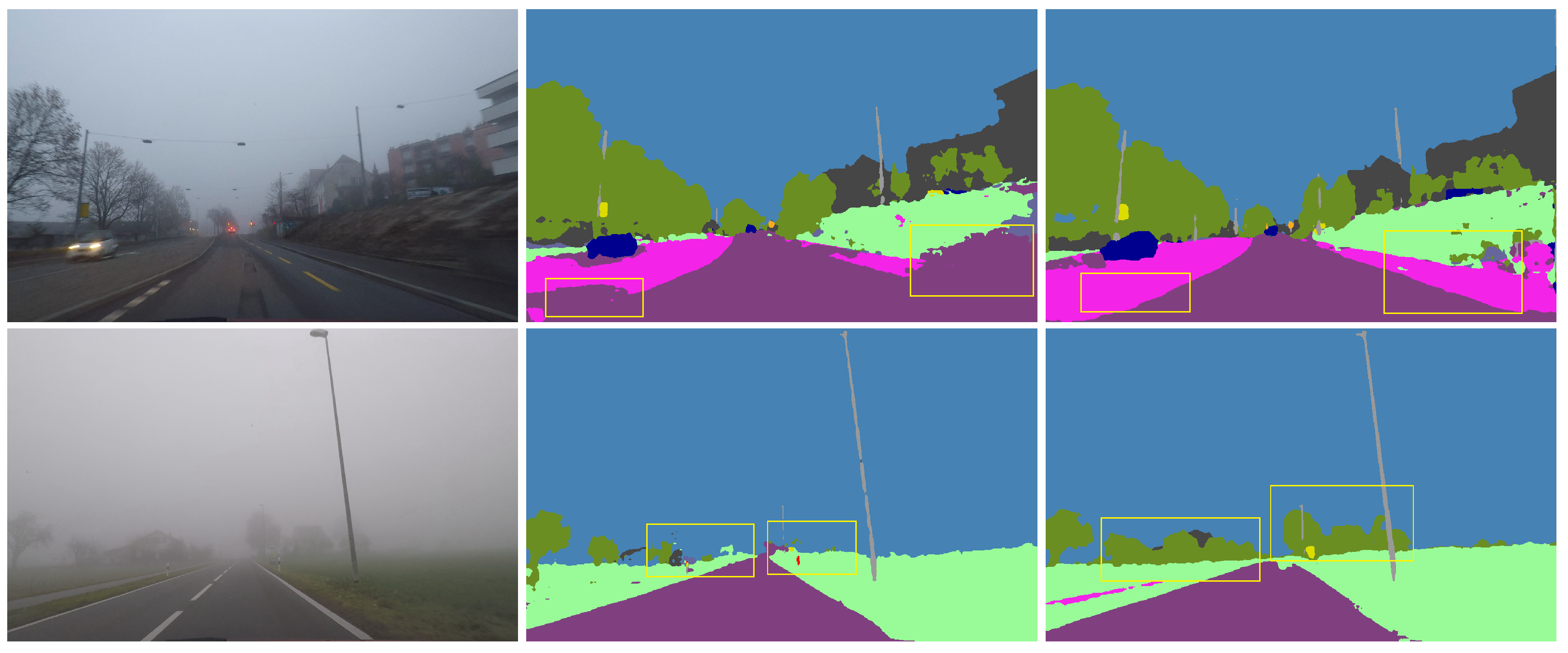
4.5. Sensitivity Analysis/Adaptability to Fog

We did not design additional modules specifically for fog processing, but our method demonstrated excellent anti-fog interference performance, which was analyzed using entropy. The brighter the pixels in the entropy map, the higher the uncertainty, indicating that the model was more likely to make incorrect judgments. Conversely, the model output more certain segmentation results. However, the model also generated high-certainty but incorrect segmentation. Therefore, only the segmentation models that resulted in low entropy predictions and conformed to the distribution of the real-world scenario were truly notable. We performed predictive entropy analysis on the images from the Foggy Driving Dense dataset [37], as shown in Figure 8. The baseline model DAFormer [25] made highly uncertain predictions on fog-obscured pixels, potentially leading to unsafe situations. SDAT-Former alleviated this but still retained uncertainty. In contrast, our model generated lower uncertainty in dense fog conditions while still producing accurate road and sky segmentation results, demonstrating the exceptional reliability of our method.

4.6. Number of Images from the Intermediate Domain

We explored the effect of intermediate domain images with varying quantities from different datasets, which is shown in

Table 4. Discussion about the usage of intermediate domain images. We chose different numbers of clear images from the different datasets, denoted as $\mathcal{M}$. The results are measured by the mIoU (%).

Discussion of Numbers					mIoU
Number of images from intermediate domain	400 ${}^1$	600 ${}^2$	1000 ${}^3$	1600 ${}^4$	ACDC	FZ
	✓				56.19	47.42
		✓			54.17	51.61
			✓		59.28	53.82
				✓	58.34	53.97

¹ Clear reference images from the training set of the ACDC fog dataset. ² Manually selected images from the “light fog” category in the Foggy Zurich dataset. ³ Combination of 400 images from the ACDC dataset and 600 images from the FZ dataset. ⁴ Remaining 600 reference images from the ACDC fog validation/test set.

. Firstly, using an exclusive intermediate domain led to optimal results on the current dataset but did not achieve the same performance on another dataset. For example, using intermediate domain images from the ACDC dataset resulted in a segmentor mIoU of 47.42% on the Foggy Zurich dataset. This was due to the style variations between the datasets. Secondly, in the same dataset, the number of images from the intermediate domain had little influence on the final performance. In other words, the corresponding relationship between the clear domain and the foggy domain does not need to be very strict, indicating the segmentor has adaptability in both fog-invariant feature learning and intermediate domain segmentation learning.

4.7. Generalization to Rainy and Snowy Scenes

We found that SDAT-Former++ could make better predictions for clear images (Figure 9). We used the trained SDAT-Former++ to re-predict the intermediate domain images and obtained surprisingly high-quality pseudo-labels. This indicates that the target domain is also an “extension domain” to the intermediate domain, forcing the model to complete more difficult tasks, potentially improving performance in the current task. Furthermore, we tested our method on the rain and snow validation sets of the ACDC dataset (

Table 5. Generalization to other adverse scenes. We conducted zero-shot testing on the snowy and rainy validation sets of the ACDC dataset.

Generalization on ACDC Validation Subsets		Rain	Snow
Method	SegFormer(no UDA) [39]	40.62	42.03
	DAFormer(baseline) [25]	48.27	49.19
	SDAT-Former [1]	53.99	58.04
	SDAT-Former++	56.83	60.14

and Figure 9), showing improvements compared to DAFormer, indicating the potential of our method in addressing the understanding of different adverse scenes.

4.8. Order of EMA Updating

EMA updating is a temporal ensemble algorithm, signifying that ($a(x+b)\ne ax+b$); thus, different sequences of EMA updating may affect the final parameters of the segmentor. In

Table 6. The order of EMA updating. We designed three different sequences for parameter updating.

Order of EMA Updating				mIoU	Gain
Configuration	Fi ${}^2$→T ${}^3$	S ${}^1$→T	TA ${}^4$→T	ACDC	FZ
	1	2	3	58.14	52.78
	2	1	3	59.24	53.80
	1	3	2	59.17	53.68
	1	2	3	59.28	53.82

¹ “S” represents the student segmentor $f_{\theta }$. ² “Fi” represents the fog-invariant backbone $b_{\omega }^{\mathrm{fi}}$. ³ “T” represents the teacher segmentor $h_{\phi }$. ⁴ “TA” represents the teaching-assistant backbone $b_{\psi }^{\mathrm{si}}$.

, we present the results of an ablation study on the order of EMA updating. The results show that altering the sequence of EMA updating concerning the teacher segmentor had little effect on performance, which can be attributed to cyclical training.

4.9. Memory Consumption Comparison

Our method does not require all modules to work simultaneously. We adopt cyclical training where every four iterations constitute one mini-epoch, and only two–three modules need to be executed in each iteration. Specifically, in the first and second iterations, only the student segmentor $f_{\theta }$ and the fog-related modules ($b_{\omega }^{\mathrm{fi}}$ and $\mathcal{F}$) are involved. The third iteration needs $f_{\theta }$, $b_{\psi }^{\mathrm{si}}$, and $d_r$, whereas the fourth iteration needs $f_{\theta }$ and $h_{\phi }$. The transferring of EMA parameters does not increase memory consumption. Due to the introduction of new loss functions, our method consumes more memory compared to previous methods, but it does not exceed the limit of a Tesla V100 (32 GB). During the testing phase, our method only deploys $f_{\theta }$; thus, the consumption is consistent with the original SegFormer [39]. In this context, our method is more like online knowledge distillation, aiming to train a better student network. We provide a comparison of the memory consumption between our method and DAFormer [25], SegFormer [39], and SDAT-Former [1] during the training and testing phases in

Table 7. Memory consumption comparison. We recorded the memory consumption during training and testing when batch_size =1, with an input size of $512\times 512$ for both the source domain and target domain images, measured in GB.

Memory Consumption Comparison (GB)
	Train				Test
Mini-epoch	Iter 4n	Iter 4n + 1	Iter 4n + 2	Iter 4n + 3
SegFormer [39]	5.7
DAFormer [25]	11.3				5.7
SDAT-Former [1]	5.9	7.7	8.3	11.9
SDAT-Former++	6.4	8.5	9.4	13.3

.

5. Conclusions

We propose a stronger domain-adaptive teacher-guided semantic segmentation method called SDAT-Former++. It improves both style-invariant and fog-invariant feature learning. Specifically, we replace the strategy of generating pseudo-labels using supervised learning with a simple yet effective masked learning strategy. This integrates all training processes into an end-to-end framework, greatly simplifying the training process and improving performance. Furthermore, we enhance the fog-invariant feature learning module by introducing positional encoding, guiding the model to learn more refined fog-related features and scene contours. In the information integration part, we use consistency learning to accelerate model convergence and narrow the gap between the student and teacher segmentors.

Experimental results demonstrate that SDAT-Former++ surpasses the baseline methods on mainstream foggy road scene datasets. It achieves improvements of 3.3%, 4.8%, 1.1%, and 0.4% on the ACDC Fog, Foggy Zurich, Foggy Driving, and Foggy Driving Dense datasets, respectively. Through analysis of the model outputs, we find that both intermediate domain learning and fog-invariant feature learning in SDAT-Former++ have positive effects, alleviating the issue of prediction artifacts in the baseline methods. When facing dense fog, the proposed method exhibits lower uncertainty and demonstrates good safety performance. Visualizing the model’s feature maps also reveals that intermediate domain data primarily focuses on learning domain-style independent features (such as contours and edges), whereas fog-invariant feature learning differentiates between fog and entities in the images. Masked learning enables the model to better capture contextual information rather than specific details, and positional encoding generates better contour information, assisting the main segmentation model in producing better edges. Our method also shows generalization ability to other adverse scenes such as rainy and snowy scenes.

In future studies, we plan to further research the fog factor and attempt to more accurately avoid its influence. We also plan to research the unified segmentor, which is suitable for all adverse conditions.

References

1. Wang, Z.; Zhang, Y.; Yu, Y.; Jiang, Z. SDAT-Former: Foggy Scene Semantic Segmentation Via A Strong Domain Adaptation Teacher. In Proceedings of the 2023 IEEE International Conference on Image Processing (ICIP), Kuala Lumpur, Malaysia, 8–11 October 2023; pp. 1760–1764. [Google Scholar] [CrossRef]
2. Ranft, B.; Stiller, C. The Role of Machine Vision for Intelligent Vehicles. IEEE Trans. Intell. Veh. 2016, 1, 8–19. [Google Scholar] [CrossRef]
3. Dai, Y.; Li, C.; Su, X.; Liu, H.; Li, J. Multi-Scale Depthwise Separable Convolution for Semantic Segmentation in Street–Road Scenes. Remote Sens. 2023, 15, 2649. [Google Scholar] [CrossRef]
4. Liu, Q.; Dong, Y.; Jiang, Z.; Pei, Y.; Zheng, B.; Zheng, L.; Fu, Z. Multi-Pooling Context Network for Image Semantic Segmentation. Remote Sens. 2023, 15, 2800. [Google Scholar] [CrossRef]
5. Šarić, J.; Oršić, M.; Šegvić, S. Panoptic SwiftNet: Pyramidal Fusion for Real-Time Panoptic Segmentation. Remote Sens. 2023, 15, 1968. [Google Scholar] [CrossRef]
6. Lv, K.; Zhang, Y.; Yu, Y.; Zhang, Z.; Li, L. Visual Localization and Target Perception Based on Panoptic Segmentation. Remote Sens. 2022, 14, 3983. [Google Scholar] [CrossRef]
7. Li, X.; Xu, F.; Lyu, X.; Gao, H.; Tong, Y.; Cai, S.; Li, S.; Liu, D. Dual attention deep fusion semantic segmentation networks of large-scale satellite remote-sensing images. Int. J. Remote Sens. 2021, 42, 3583–3610. [Google Scholar] [CrossRef]
8. Li, X.; Xu, F.; Xia, R.; Li, T.; Chen, Z.; Wang, X.; Xu, Z.; Lyu, X. Encoding contextual information by interlacing transformer and convolution for remote sensing imagery semantic segmentation. Remote Sens. 2022, 14, 4065. [Google Scholar] [CrossRef]
9. Li, X.; Xu, F.; Liu, F.; Xia, R.; Tong, Y.; Li, L.; Xu, Z.; Lyu, X. Hybridizing Euclidean and Hyperbolic Similarities for Attentively Refining Representations in Semantic Segmentation of Remote Sensing Images. IEEE Geosci. Remote Sens. Lett. 2022, 19, 1–5. [Google Scholar] [CrossRef]
10. Li, X.; Xu, F.; Liu, F.; Lyu, X.; Tong, Y.; Xu, Z.; Zhou, J. A Synergistical Attention Model for Semantic Segmentation of Remote Sensing Images. IEEE Trans. Geosci. Remote Sens. 2023, 61, 1–16. [Google Scholar] [CrossRef]
11. Sakaridis, C.; Dai, D.; Van Gool, L. Semantic foggy scene understanding with synthetic data. Int. J. Comput. Vis. 2018, 126, 973–992. [Google Scholar] [CrossRef]
12. Narasimhan, S.G.; Nayar, S.K. Contrast restoration of weather degraded images. IEEE Trans. Pattern Anal. Mach. Intell. 2003, 25, 713–724. [Google Scholar] [CrossRef]
13. Michieli, U.; Biasetton, M.; Agresti, G.; Zanuttigh, P. Adversarial Learning and Self-Teaching Techniques for Domain Adaptation in Semantic Segmentation. IEEE Trans. Intell. Veh. 2020, 5, 508–518. [Google Scholar] [CrossRef]
14. Cordts, M.; Omran, M.; Ramos, S.; Rehfeld, T.; Enzweiler, M.; Benenson, R.; Franke, U.; Roth, S.; Schiele, B. The cityscapes dataset for semantic urban scene understanding. In Proceedings of the IEEE conference on Computer Vision and Pattern Recognition, Las Vegas, NV, USA, 27–30 June 2016; pp. 3213–3223. [Google Scholar]
15. Goodfellow, I.; Pouget-Abadie, J.; Mirza, M.; Xu, B.; Warde-Farley, D.; Ozair, S.; Courville, A.; Bengio, Y. Generative adversarial networks. Commun. ACM 2020, 63, 139–144. [Google Scholar] [CrossRef]
16. Lee, D.H. Pseudo-label: The simple and efficient semi-supervised learning method for deep neural networks. In Proceedings of the Workshop on Challenges in Representation Learning, ICML, Atlanta, GA, USA, 16–21 June 2013; Volume 3, p. 896. [Google Scholar]
17. Mao, X.; Li, Q.; Xie, H.; Lau, R.Y.K.; Wang, Z.; Smolley, S.P. Least Squares Generative Adversarial Networks. arXiv 2016, arXiv:1611.04076. [Google Scholar]
18. Hoffman, J.; Tzeng, E.; Park, T.; Zhu, J.Y.; Isola, P.; Saenko, K.; Efros, A.A.; Darrell, T. CyCADA: Cycle-Consistent Adversarial Domain Adaptation. Computer Vision and Pattern Recognition arXiv 2017, arXiv:1711.03213v3. [Google Scholar]
19. Chang, W.L.; Wang, H.P.; Peng, W.H.; Chiu, W.C. All about structure: Adapting structural information across domains for boosting semantic segmentation. In Proceedings of the IEEE/CVF Conference on Computer Vision and Pattern Recognition, Long Beach, CA, USA, 15–20 June 2019; pp. 1900–1909. [Google Scholar]
20. Tsai, Y.H.; Hung, W.C.; Schulter, S.; Sohn, K.; Yang, M.H.; Chandraker, M. Learning to adapt structured output space for semantic segmentation. In Proceedings of the IEEE Conference on Computer Vision and Pattern Recognition, Salt Lake City, UT, USA, 18–23 June 2018; pp. 7472–7481. [Google Scholar]
21. Vu, T.H.; Jain, H.; Bucher, M.; Cord, M.; Pérez, P. Advent: Adversarial entropy minimization for domain adaptation in semantic segmentation. In Proceedings of the IEEE/CVF Conference on Computer Vision and Pattern Recognition, Long Beach, CA, USA, 15–20 June 2019; pp. 2517–2526. [Google Scholar]
22. Zou, Y.; Yu, Z.; Liu, X.; Kumar, B.V.; Wang, J. Confidence Regularized Self-Training. In Proceedings of the IEEE International Conference on Computer Vision (ICCV), Seoul, Republic of Korea, 27 October–2 November 2019. [Google Scholar]
23. Tranheden, W.; Olsson, V.; Pinto, J.; Svensson, L. Dacs: Domain adaptation via cross-domain mixed sampling. In Proceedings of the IEEE/CVF Winter Conference on Applications of Computer Vision, Virtual, 5–9 January 2021; pp. 1379–1389. [Google Scholar]
24. Zhang, P.; Zhang, B.; Zhang, T.; Chen, D.; Wang, Y.; Wen, F. Prototypical pseudo label denoising and target structure learning for domain adaptive semantic segmentation. In Proceedings of the IEEE/CVF Conference on Computer vision and Pattern Recognition, Nashville, TN, USA, 20–25 June 2021; pp. 12414–12424. [Google Scholar]
25. Hoyer, L.; Dai, D.; Van Gool, L. Daformer: Improving network architectures and training strategies for domain-adaptive semantic segmentation. In Proceedings of the IEEE/CVF Conference on Computer Vision and Pattern Recognition, New Orleans, LA, USA, 18–24 June 2022; pp. 9924–9935. [Google Scholar]
26. Ma, X.; Wang, Z.; Zhan, Y.; Zheng, Y.; Wang, Z.; Dai, D.; Lin, C.W. Both style and fog matter: Cumulative domain adaptation for semantic foggy scene understanding. In Proceedings of the IEEE/CVF Conference on Computer Vision and Pattern Recognition, New Orleans, LA, USA, 18–24 June 2022; pp. 18922–18931. [Google Scholar]
27. Dai, D.; Sakaridis, C.; Hecker, S.; Van Gool, L. Curriculum model adaptation with synthetic and real data for semantic foggy scene understanding. Int. J. Comput. Vis. 2020, 128, 1182–1204. [Google Scholar] [CrossRef]
28. Dai, D.; Gool, L.V. Dark Model Adaptation: Semantic Image Segmentation from Daytime to Nighttime. Computer Vision and Pattern Recognition. arXiv 2018, arXiv:1810.02575. [Google Scholar]
29. Bruggemann, D.; Sakaridis, C.; Truong, P.; Gool, L.V. Refign: Align and Refine for Adaptation of Semantic Segmentation to Adverse Conditions. In Proceedings of the IEEE/CVF Winter Conference on Applications of Computer Vision, Waikoloa, HI, USA, 2–7 January 2023; pp. 3174–3184. [Google Scholar]
30. Li, Y.; Yuan, L.; Vasconcelos, N. Bidirectional learning for domain adaptation of semantic segmentation. In Proceedings of the IEEE/CVF Conference on Computer Vision and Pattern Recognition, Long Beach, CA, USA, 16–17 June 2019; pp. 6936–6945. [Google Scholar]
31. Laine, S.; Aila, T. Temporal ensembling for semi-supervised learning. arXiv 2016, arXiv:1610.02242. [Google Scholar]
32. He, K.; Chen, X.; Xie, S.; Li, Y.; Dollár, P.; Girshick, R. Masked autoencoders are scalable vision learners. In Proceedings of the IEEE/CVF Conference on Computer Vision and Pattern Recognition, New Orleans, LA, USA, 18–24 June 2022; pp. 16000–16009. [Google Scholar]
33. Hoyer, L.; Dai, D.; Wang, H.; Van Gool, L. MIC: Masked image consistency for context-enhanced domain adaptation. In Proceedings of the IEEE/CVF Conference on Computer Vision and Pattern Recognition, Vancouver, BC, Canada, 18–22 June 2023; pp. 11721–11732. [Google Scholar]
34. Dosovitskiy, A.; Beyer, L.; Kolesnikov, A.; Weissenborn, D.; Zhai, X.; Unterthiner, T.; Dehghani, M.; Minderer, M.; Heigold, G.; Gelly, S.; et al. An image is worth 16x16 words: Transformers for image recognition at scale. arXiv 2020, arXiv:2010.11929. [Google Scholar]
35. Wang, Z.; Wu, S.; Xie, W.; Chen, M.; Prisacariu, V.A. NeRF–: Neural radiance fields without known camera parameters. arXiv 2021, arXiv:2102.07064. [Google Scholar]
36. Christos, S.; Dengxin, D.; Luc, V.G. ACDC: The adverse conditions dataset with correspondences for semantic driving scene understanding. In Proceedings of the IEEE/CVF International Conference on Computer Vision, Montreal, BC, Canada, 11–17 October 2021; pp. 10765–10775. [Google Scholar]
37. Sakaridis, C.; Dai, D.; Hecker, S.; Van Gool, L. Model adaptation with synthetic and real data for semantic dense foggy scene understanding. In Proceedings of the European Conference on Computer Vision (ECCV), Munich, Germany, 8–14 September 2018; pp. 687–704. [Google Scholar]
38. Lee, S.; Son, T.; Kwak, S. Fifo: Learning fog-invariant features for foggy scene segmentation. In Proceedings of the IEEE/CVF Conference on Computer Vision and Pattern Recognition, New Orleans, LA, USA, 18–24 June 2022; pp. 18911–18921. [Google Scholar]
39. Xie, E.; Wang, W.; Yu, Z.; Anandkumar, A.; Alvarez, J.M.; Luo, P. SegFormer: Simple and efficient design for semantic segmentation with transformers. Adv. Neural Inf. Process. Syst. 2021, 34, 12077–12090. [Google Scholar]
40. Chen, L.C.; Zhu, Y.; Papandreou, G.; Schroff, F.; Adam, H. Encoder-decoder with atrous separable convolution for semantic image segmentation. In Proceedings of the European Conference on Computer Vision (ECCV), Munich, Germany, 8–14 September 2018; pp. 801–818. [Google Scholar]
41. Gong, R.; Wang, Q.; Danelljan, M.; Dai, D.; Van Gool, L. Continuous Pseudo-Label Rectified Domain Adaptive Semantic Segmentation With Implicit Neural Representations. In Proceedings of the IEEE/CVF Conference on Computer Vision and Pattern Recognition, Vancouver, BC, Canada, 18–22 June 2023; pp. 7225–7235. [Google Scholar]
42. French, G.; Laine, S.; Aila, T.; Mackiewicz, M.; Finlayson, G. Semi-supervised semantic segmentation needs strong, varied perturbations. arXiv 2019, arXiv:1906.01916. [Google Scholar]
43. Olsson, V.; Tranheden, W.; Pinto, J.; Svensson, L. Classmix: Segmentation-based data augmentation for semi-supervised learning. In Proceedings of the IEEE/CVF Winter Conference on Applications of Computer Vision, Virtual, 5–9 January 2021; pp. 1369–1378. [Google Scholar]
44. Jin, Y.; Wang, J.; Lin, D. Semi-supervised semantic segmentation via gentle teaching assistant. Adv. Neural Inf. Process. Syst. 2022, 35, 2803–2816. [Google Scholar]
45. Contributors, M. MMSegmentation: Openmmlab Semantic Segmentation Toolbox and Benchmark, 2020. Available online: https://gitee.com/open-mmlab/mmsegmentation (accessed on 9 December 2023).
46. Paszke, A.; Gross, S.; Massa, F.; Lerer, A.; Bradbury, J.; Chanan, G.; Killeen, T.; Lin, Z.; Gimelshein, N.; Antiga, L.; et al. Pytorch: An imperative style, high-performance deep learning library. Adv. Neural Inf. Process. Syst. 2019, 32. [Google Scholar]
47. Deng, J.; Dong, W.; Socher, R.; Li, L.J.; Li, K.; Fei-Fei, L. Imagenet: A large-scale hierarchical image database. In Proceedings of the 2009 IEEE Conference on Computer Vision and Pattern Recognition, Miami, FL, USA, 20–25 June 2009; IEEE: Manhattan, NY, USA, 2009; pp. 248–255. [Google Scholar]
48. Loshchilov, I.; Hutter, F. Decoupled weight decay regularization. arXiv 2017, arXiv:1711.05101. [Google Scholar]
49. Chen, L.C.; Papandreou, G.; Kokkinos, I.; Murphy, K.; Yuille, A.L. Deeplab: Semantic image segmentation with deep convolutional nets, atrous convolution, and fully connected crfs. IEEE Trans. Pattern Anal. Mach. Intell. 2017, 40, 834–848. [Google Scholar] [CrossRef] [PubMed]
50. Lin, G.; Milan, A.; Shen, C.; Reid, I. Refinenet: Multi-path refinement networks for high-resolution semantic segmentation. In Proceedings of the IEEE Conference on Computer Vision and Pattern Recognition, Honolulu, HI, USA, 21–26 July 2017; pp. 1925–1934. [Google Scholar]
51. Kerim, A.; Chamone, F.; Ramos, W.; Marcolino, L.S.; Nascimento, E.R.; Jiang, R. Semantic Segmentation under Adverse Conditions: A Weather and Nighttime-aware Synthetic Data-based Approach. arXiv 2022, arXiv:2210.05626. [Google Scholar]
52. Zhang, H.; Patel, V.M. Densely Connected Pyramid Dehazing Network. arXiv 2018, arXiv:1803.08396. [Google Scholar]
53. Ren, W.; Liu, S.; Zhang, H.; Pan, J.; Cao, X.; Yang, M.H. Single image dehazing via multi-scale convolutional neural networks. In Proceedings of the Computer Vision—ECCV 2016: 14th European Conference, Amsterdam, The Netherlands, 11–14 October 2016; Proceedings, Part II 14. Springer: Berlin/Heidelberg, Germany, 2016; pp. 154–169. [Google Scholar]
54. He, K.; Sun, J.; Tang, X. Single image haze removal using dark channel prior. IEEE Trans. Pattern Anal. Mach. Intell. 2010, 33, 2341–2353. [Google Scholar]
55. Yang, Y.; Soatto, S. Fda: Fourier domain adaptation for semantic segmentation. In Proceedings of the IEEE/CVF Conference on Computer Vision and Pattern Recognition, Seattle, WA, USA, 13–19 June 2020; pp. 4085–4095. [Google Scholar]
56. Berman, D.; Avidan, S. Non-local image dehazing. In Proceedings of the IEEE Conference on Computer Vision and Pattern Recognition, Las Vegas, NV, USA, 27–30 June 2016; pp. 1674–1682. [Google Scholar]
57. Benjdira, B.; Ali, A.M.; Koubaa, A. Streamlined Global and Local Features Combinator (SGLC) for High Resolution Image Dehazing. In Proceedings of the IEEE/CVF Conference on Computer Vision and Pattern Recognition, Vancouver, BC, Canada, 18–22 June 2023; pp. 1854–1863. [Google Scholar]
Figure 1. The main idea of the proposed method. Unlike the original SDAT-Former, we optimize the learning of style information and add feature enhancement for fog-invariant feature learning, greatly reducing the computing consumption and integrating the processing pipeline. We also add consistency learning and dynamic weighting when processing the knowledge transfer.
Remotesensing 15 05704 g001
Figure 2. The overall workflow of our method. (Left) Training flow within a mini-epoch that can be repeated as the base training unit. (Right) The sub-process (AE) includes learning segmentation and style knowledge from the source and intermediate domains (A,C), attempting to train the backbone producing fog-invariant features adversarially (B.1,B.2), transferring all knowledge to the teacher (D), and compelling it to generate better pseudo-labels for supervision (E).
Remotesensing 15 05704 g002
Figure 3. Qualitative comparison with other methods. Since the ground truths from the ACDC-test dataset were withheld and the fog in the images from the Foggy Driving dataset was light, we randomly selected images from the challenging Foggy Driving Dense dataset (top three lines) and Foggy Zurich-test dataset (bottom three lines) with dense fog to compare the performance of our method with that of other methods.
Remotesensing 15 05704 g003
Figure 4. Qualitative results of ablation study. These experiments were conducted on the Foggy Zurich-test dataset. Both points (i.e., intermediate domain style learning (Column 3) and fog-invariant feature learning (Column 4)) yielded significant improvements compared to the baseline.
Remotesensing 15 05704 g004
Figure 5. Qualitative results for the incorporation of positional encoding in fog-invariant learning. From left to right: input image, performance without/with position encoding. Compared to the original method [1], our method can better overcome incomplete segmentation caused by motion blur and effectively identify objects obscured by dense fog.
Remotesensing 15 05704 g005
Figure 6. Qualitative comparison of using masked learning in the intermediate domain. From left to right: Input image, bad prediction by SDAT-Former [1], refined prediction by our method. The original version uses style transfer, which can inevitably lead to artifacts in predictions, whereas SDAT-Former++ does not.
Remotesensing 15 05704 g006
Figure 7. Qualitative feature maps of b ψ si and b ω fi . From left to right: intermediate domain image, output of b ψ si without masked learning (SDAT-Former [1]) and the case with it, target domain image, output of b ω fi without and with positional encoding.
Remotesensing 15 05704 g007
Figure 8. Entropy analysis. From left to right: input images (dense fog), entropy map output by DAFormer [25], entropy map output by SDAT-Former [1], and entropy map output by our method. Our method resulted in lower prediction entropy for the pixels occupied by fog, indicating higher confidence in its predictions.
Remotesensing 15 05704 g008
Figure 9. Qualitative results of generalization on rainy and snowy images. From left to right: input images, predictions of DAFormer [25], predictions of SDAT-Former [1], and predictions of our method. These experiments were conducted on the ACDC rain and snow subsets. We directly used the checkpoint acquired by this paper to test without any extra training. The newly proposed SDAT-Former++ greatly improved segmentation compared to DAFormer and the original SDAT-Former.
Remotesensing 15 05704 g009