

Automated Recognition of Tree Species Composition of Forest Communities Using Sentinel-2 Satellite Data


Abstract
1. Introduction
2. Materials and Methods
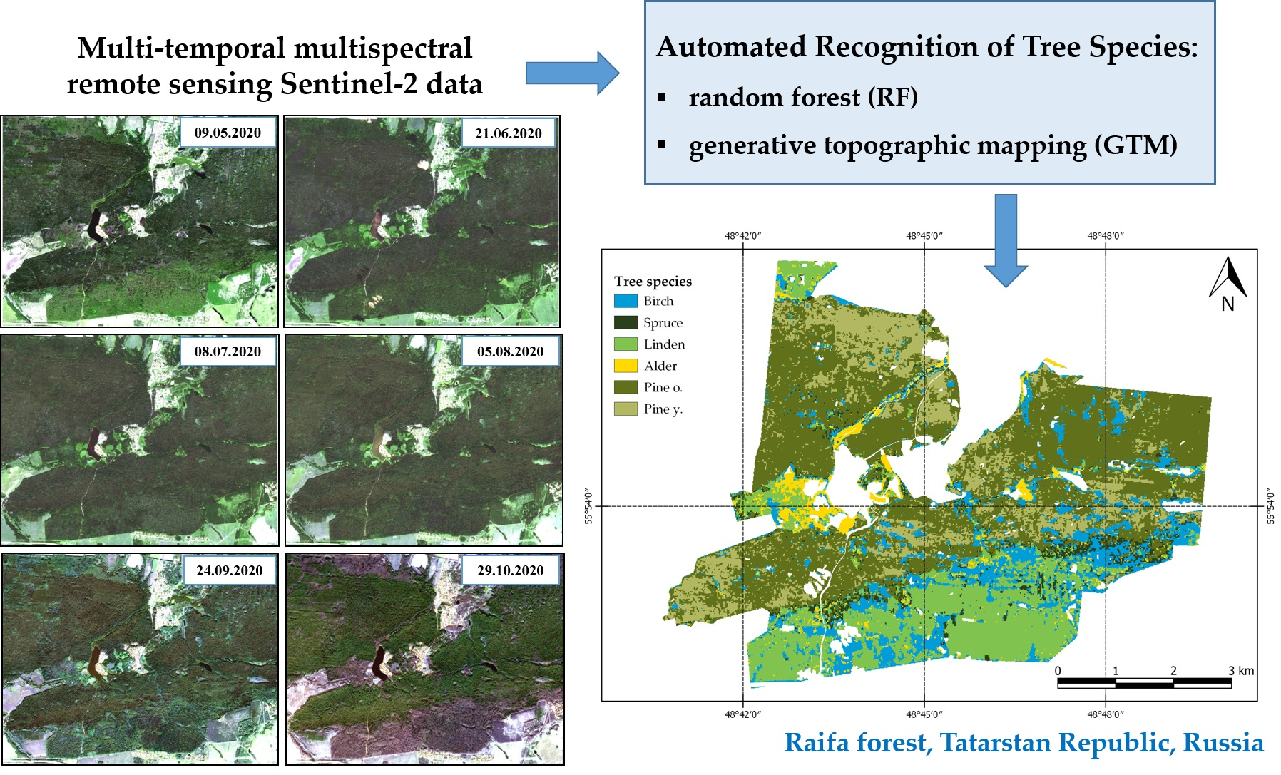
2.1. Study Area
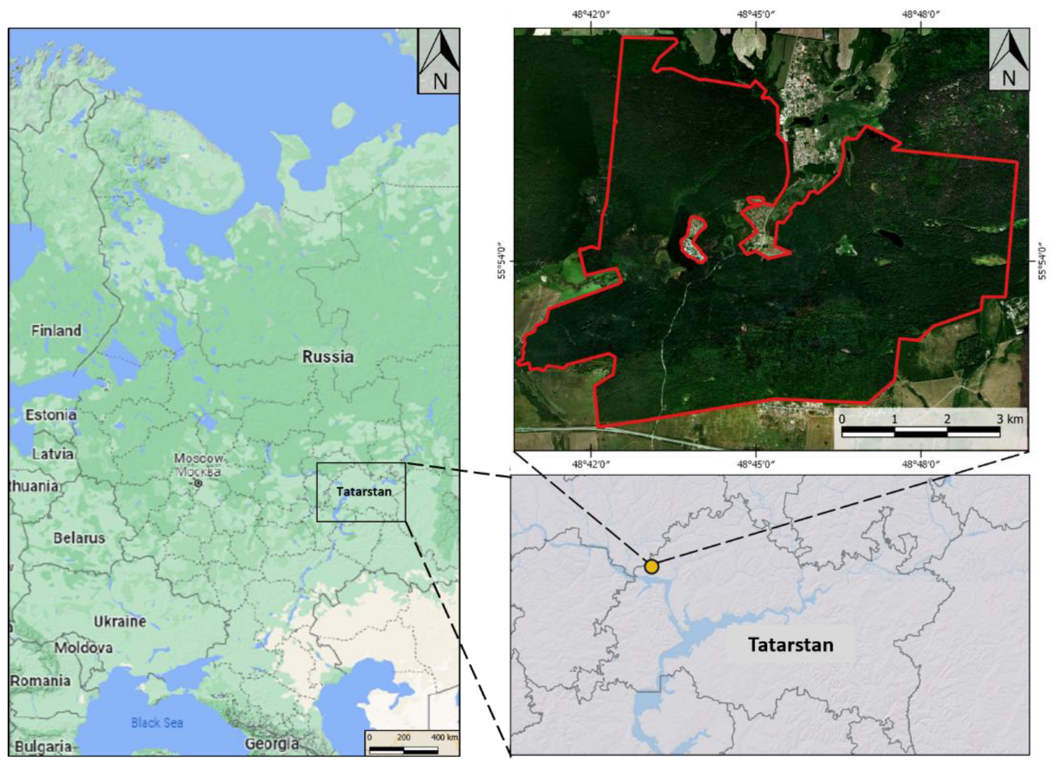
2.2. Ground Data
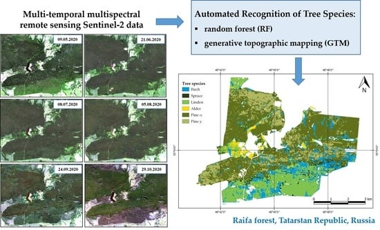
2.3. Remote Sensing Data
2.4. Training Sample
2.5. Spectral Properties Analysis
2.6. Recognition Methods
2.7. Accuracy Assessment
3. Results
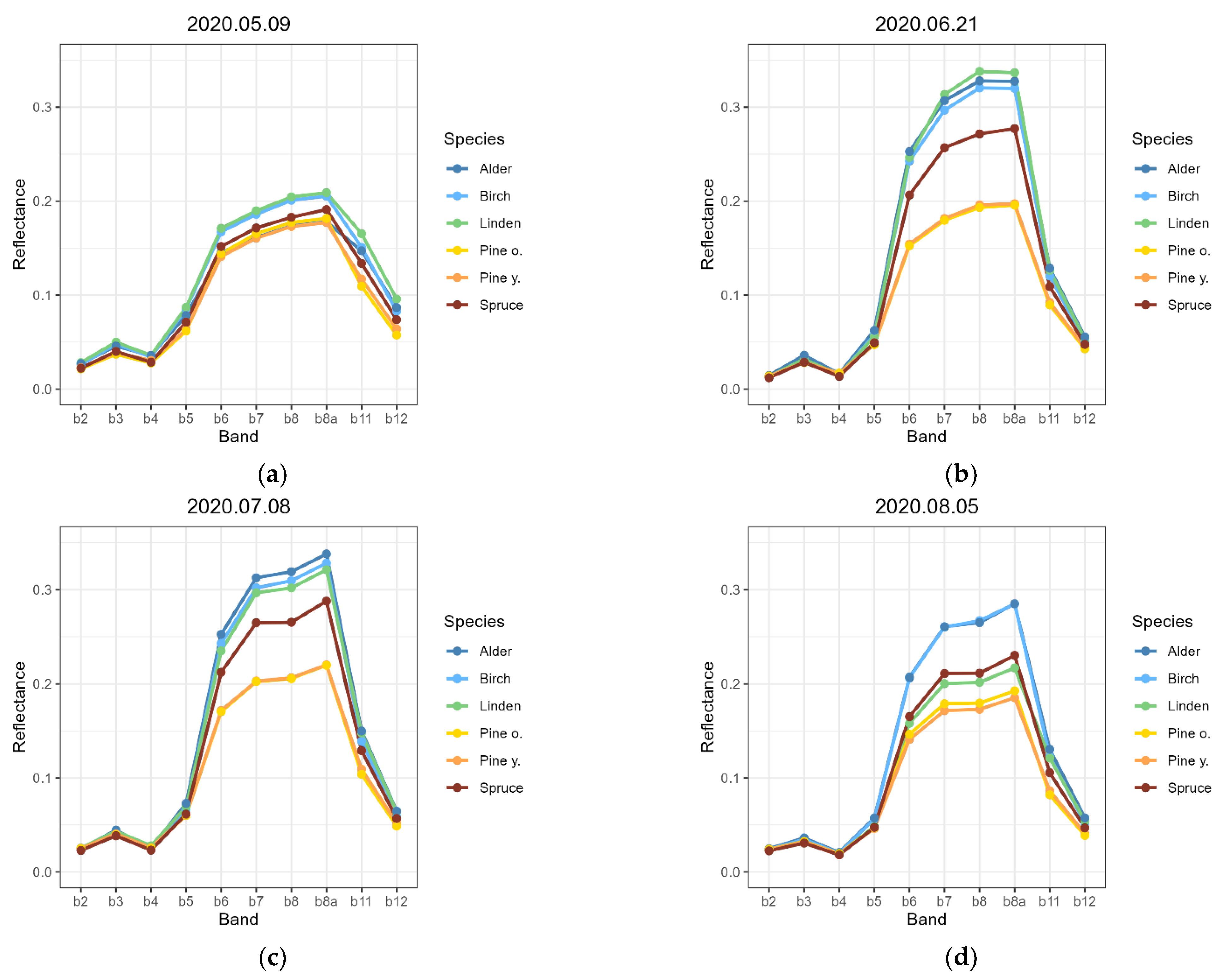
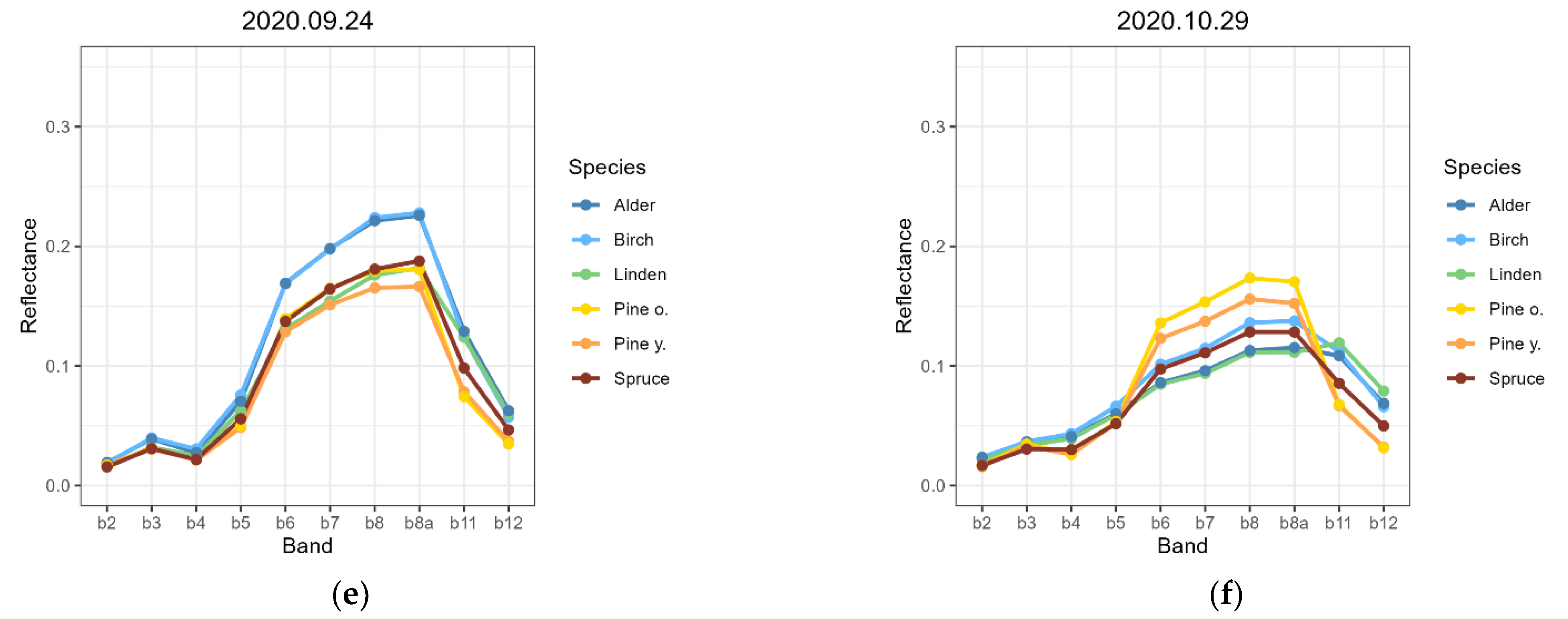
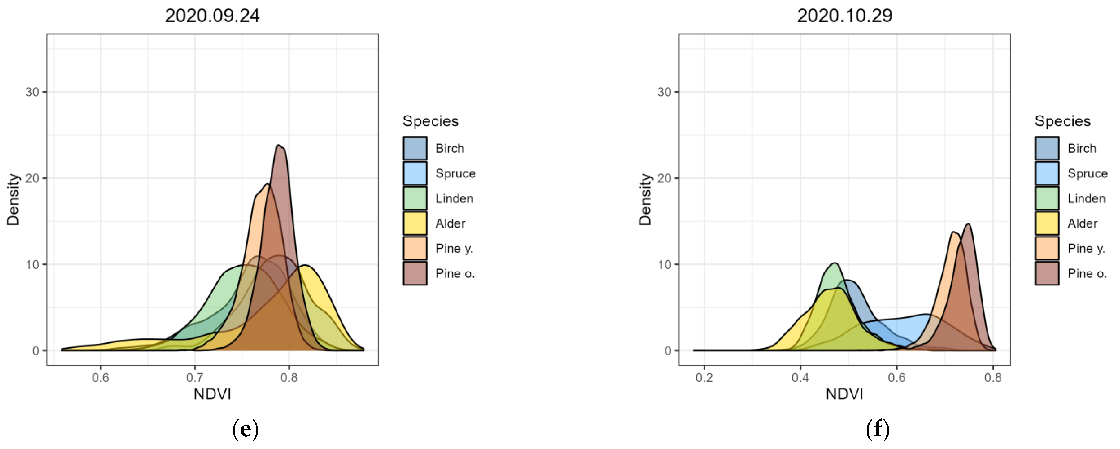
3.1. Spectral Properties of the Studied Tree Species
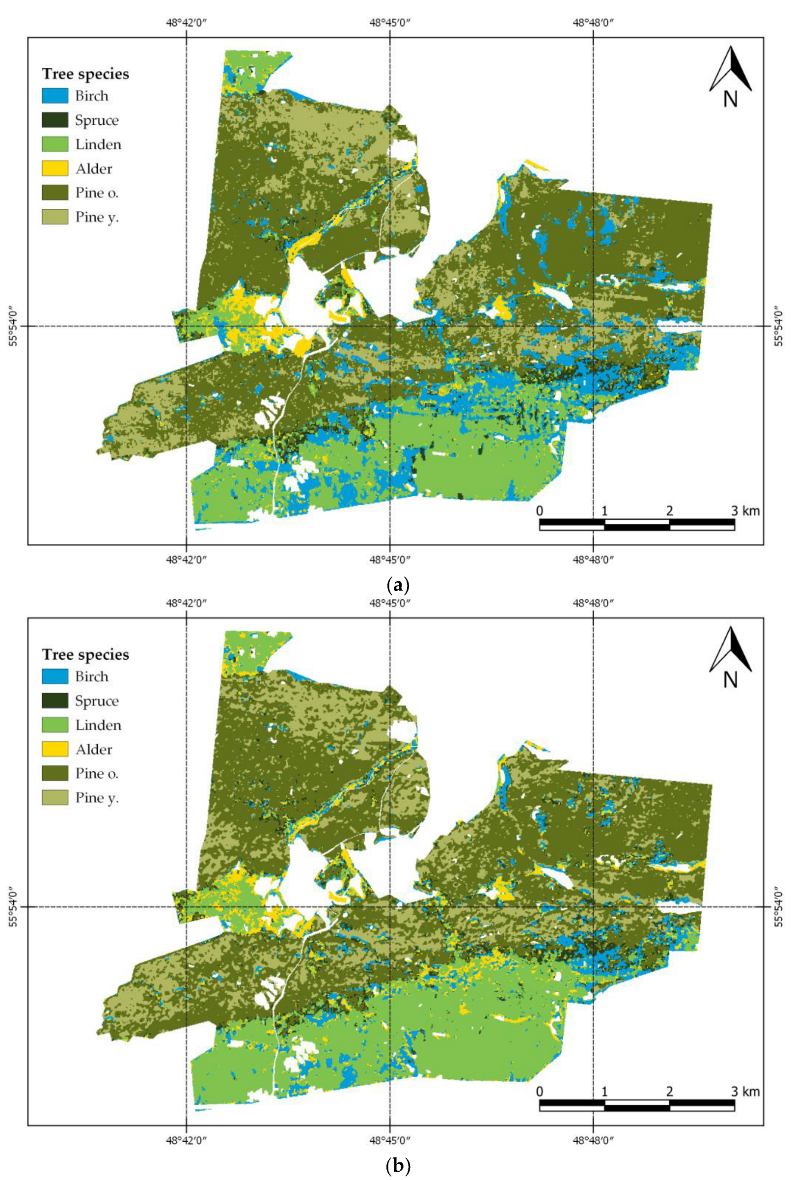
3.2. Automated Recognition of Tree Species
3.3. Recognition Quality Assessment
4. Discussion
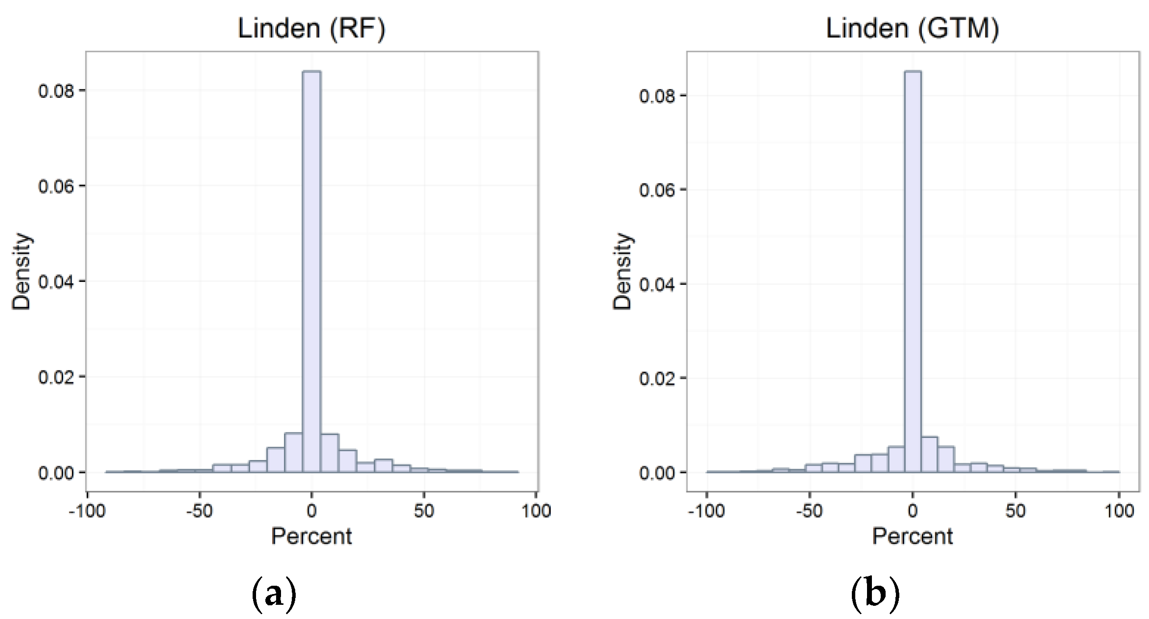
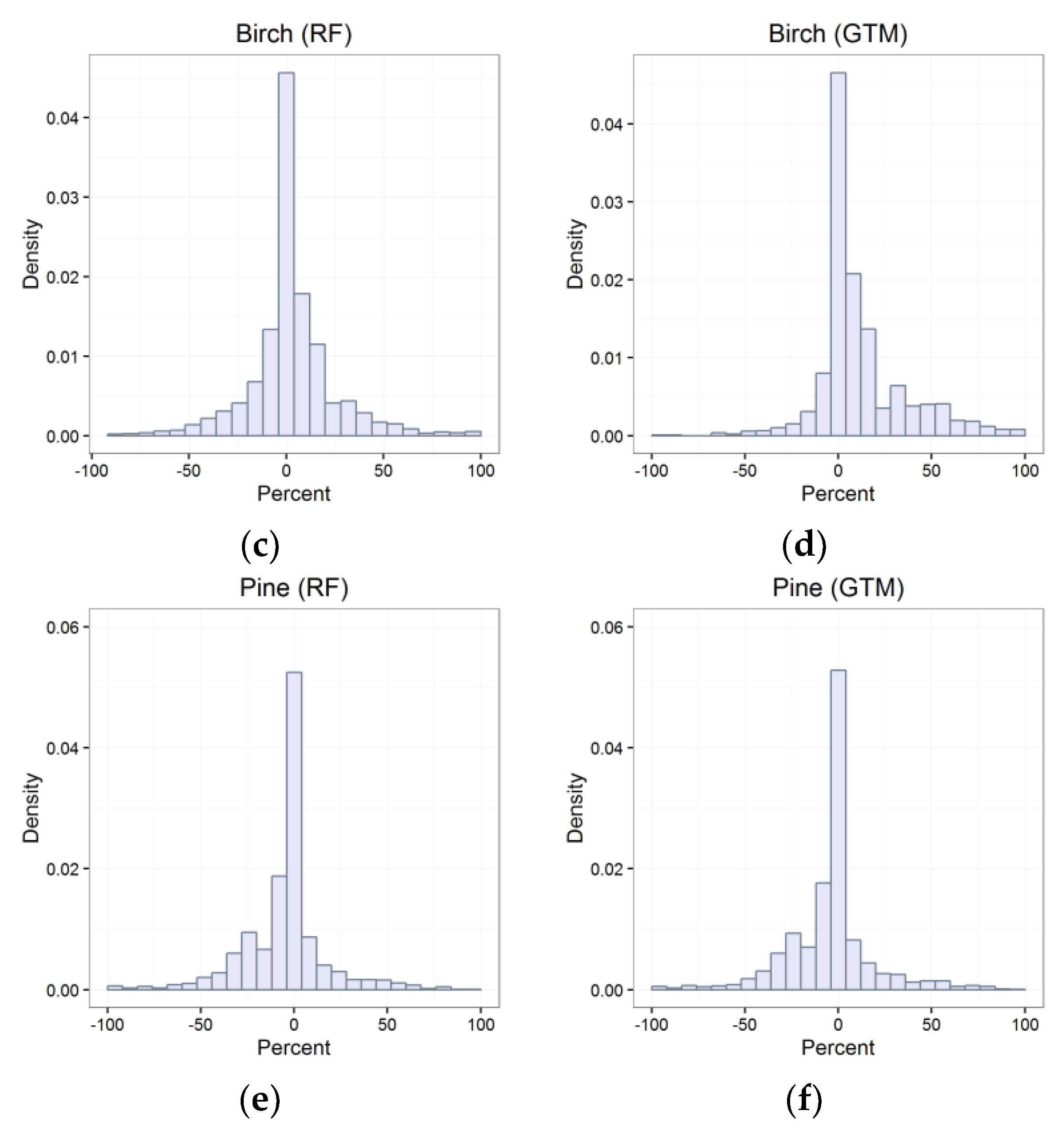
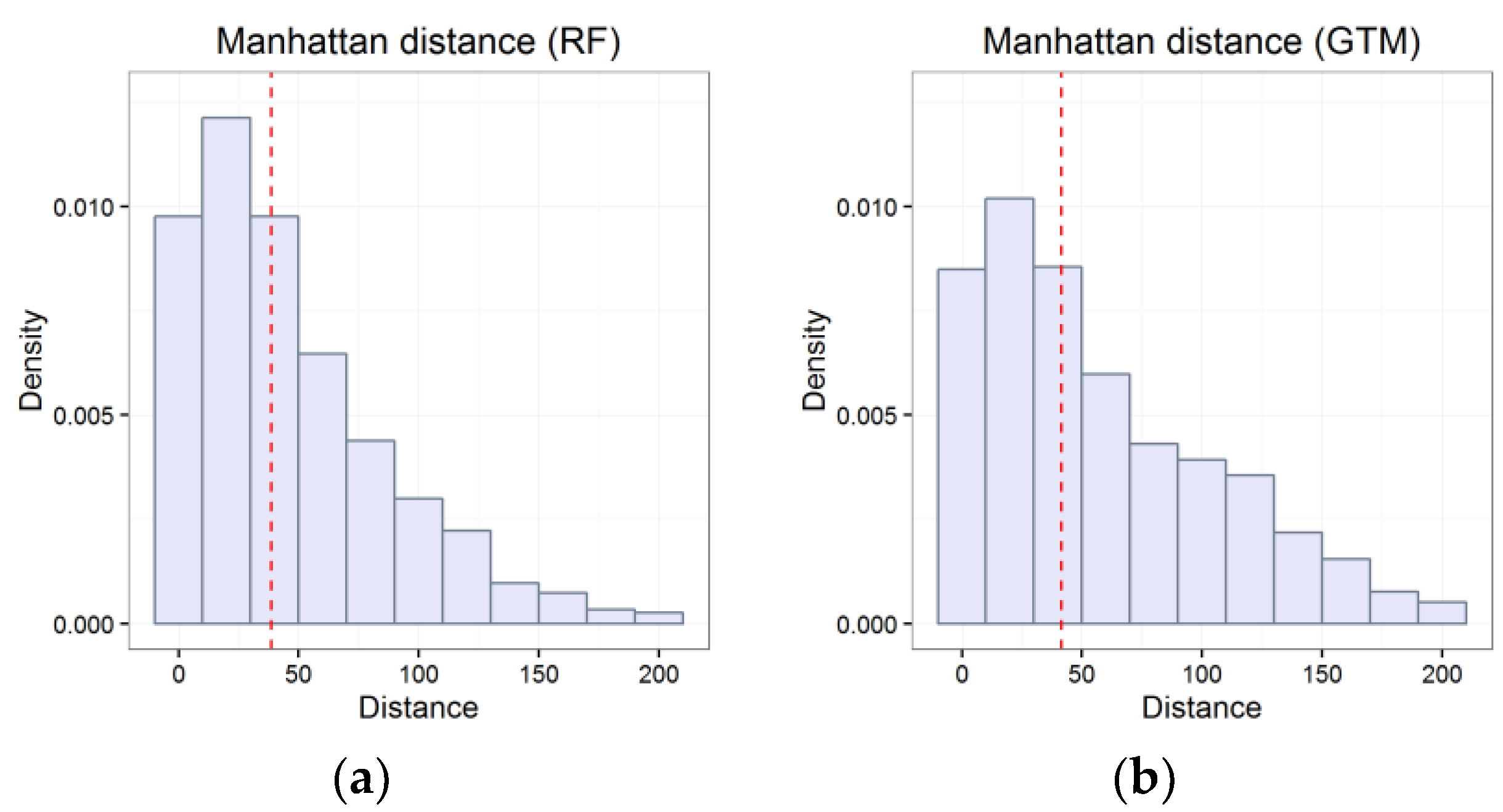
4.1. Validation of Results
4.2. Limiations and Further Study
5. Conclusions
Author Contributions
Funding
Data Availability Statement
Acknowledgments
Conflicts of Interest
References
- Westoby, J.C. Introduction to World Forestry: People and Their Trees; B. Blackwell: Oxford, UK; New York, NY, USA, 1989; ISBN 978-0-631-16133-2. [Google Scholar]
- Global Environmental Change: Research Pathways for the Next Decade; National Research Council (U.S.), Ed.; National Academy Press: Washington, DC, USA, 1999; ISBN 978-0-309-06420-0. [Google Scholar]
- Fassnacht, F.E.; Latifi, H.; Stereńczak, K.; Modzelewska, A.; Lefsky, M.; Waser, L.T.; Straub, C.; Ghosh, A. Review of Studies on Tree Species Classification from Remotely Sensed Data. Remote Sens. Environ. 2016, 186, 64–87. [Google Scholar] [CrossRef]
- Felbermeier, B.; Hahn, A.; Schneider, T. Study on User Requirements for Remote Sensing Applications in Forestry. In Proceedings of the ISPRS TC VII Symposium—100 Years ISPRS, Vienna, Austria, 5–7 July 2010; Volume 38, pp. 210–212. [Google Scholar]
- Xie, Y.; Sha, Z.; Yu, M. Remote Sensing Imagery in Vegetation Mapping: A Review. J. Plant Ecol. 2008, 1, 9–23. [Google Scholar] [CrossRef]
- European Space Agency Sentinel-2 User Handbook: Standard Document 2015. Available online: https://sentinel.esa.int/documents/247904/685211/sentinel-2_user_handbook (accessed on 29 November 2022).
- Bolyn, C.; Michez, A.; Gaucher, P.; Lejeune, P.; Bonnet, S. Forest mapping and species composition using supervised per pixel classification of Sentinel-2 imagery. Biotechnol. Agron. Soc. Environ. 2018, 22, 172–187. [Google Scholar] [CrossRef]
- Grabska, E.; Hostert, P.; Pflugmacher, D.; Ostapowicz, K. Forest Stand Species Mapping Using the Sentinel-2 Time Series. Remote Sens. 2019, 11, 1197. [Google Scholar] [CrossRef]
- Immitzer, M.; Vuolo, F.; Atzberger, C. First Experience with Sentinel-2 Data for Crop and Tree Species Classifications in Central Europe. Remote Sens. 2016, 8, 166. [Google Scholar] [CrossRef]
- Persson, M.; Lindberg, E.; Reese, H. Tree Species Classification with Multi-Temporal Sentinel-2 Data. Remote Sens. 2018, 10, 1794. [Google Scholar] [CrossRef]
- Wessel, M.; Brandmeier, M.; Tiede, D. Evaluation of Different Machine Learning Algorithms for Scalable Classification of Tree Types and Tree Species Based on Sentinel-2 Data. Remote Sens. 2018, 10, 1419. [Google Scholar] [CrossRef]
- Addabbo, P.; Focareta, M.; Marcuccio, S.; Votto, C.; Ullo, S.L. Contribution of Sentinel-2 Data for Applications in Vegetation Monitoring. Acta Imeko 2016, 5, 44. [Google Scholar] [CrossRef]
- Pinto, F.; Rouillard, D.; Sobze, J.-M.; Ter-Mikaelian, M. Validating Tree Species Composition in Forest Resource Inventory for Nipissing Forest, Ontario, Canada. For. Chron. 2007, 83, 247–251. [Google Scholar] [CrossRef]
- Magnussen, S.; Russo, G. Uncertainty in Photo-Interpreted Forest Inventory Variables and Effects on Estimates of Error in Canada’s National Forest Inventory. For. Chron. 2012, 88, 439–447. [Google Scholar] [CrossRef]
- Ballanti, L.; Blesius, L.; Hines, E.; Kruse, B. Tree Species Classification Using Hyperspectral Imagery: A Comparison of Two Classifiers. Remote Sens. 2016, 8, 445. [Google Scholar] [CrossRef]
- Immitzer, M.; Atzberger, C.; Koukal, T. Tree Species Classification with Random Forest Using Very High Spatial Resolution 8-Band WorldView-2 Satellite Data. Remote Sensing 2012, 4, 2661–2693. [Google Scholar] [CrossRef]
- Krahwinkler, P.; Rossmann, J. Tree Species Classification and Input Data Evaluation. Eur. J. Remote Sens. 2013, 46, 535–549. [Google Scholar] [CrossRef]
- Breiman, L. Random Forest. Mach. Learn. 2001, 45, 5–32. [Google Scholar] [CrossRef]
- Mellor, A.; Haywood, A.; Stone, C.; Jones, S. The Performance of Random Forests in an Operational Setting for Large Area Sclerophyll Forest Classification. Remote Sens. 2013, 5, 2838–2856. [Google Scholar] [CrossRef]
- Du, P.; Samat, A.; Waske, B.; Liu, S.; Li, Z. Random Forest and Rotation Forest for Fully Polarized SAR Image Classification Using Polarimetric and Spatial Features. ISPRS J. Photogramm. Remote Sens. 2015, 105, 38–53. [Google Scholar] [CrossRef]
- Rodriguez-Galiano, V.F.; Ghimire, B.; Rogan, J.; Chica-Olmo, M.; Rigol-Sanchez, J.P. An Assessment of the Effectiveness of a Random Forest Classifier for Land-Cover Classification. ISPRS J. Photogramm. Remote Sens. 2012, 67, 93–104. [Google Scholar] [CrossRef]
- Pal, M. Random Forest Classifier for Remote Sensing Classification. Int. J. Remote Sens. 2005, 26, 217–222. [Google Scholar] [CrossRef]
- Körting, T.S.; Garcia Fonseca, L.M.; Câmara, G. GeoDMA—Geographic Data Mining Analyst. Comput. Geosci. 2013, 57, 133–145. [Google Scholar] [CrossRef]
- Belgiu, M.; Drǎguţ, L.; Strobl, J. Quantitative Evaluation of Variations in Rule-Based Classifications of Land Cover in Urban Neighbourhoods Using WorldView-2 Imagery. ISPRS J. Photogramm. Remote Sens. 2014, 87, 205–215. [Google Scholar] [CrossRef]
- Illarionova, S.; Trekin, A.; Ignatiev, V.; Oseledets, I. Tree Species Mapping on Sentinel-2 Satellite Imagery with Weakly Supervised Classification and Object-Wise Sampling. Forests 2021, 12, 1413. [Google Scholar] [CrossRef]
- Ng, W.-T.; Rima, P.; Einzmann, K.; Immitzer, M.; Atzberger, C.; Eckert, S. Assessing the Potential of Sentinel-2 and Pléiades Data for the Detection of Prosopis and Vachellia Spp. in Kenya. Remote Sens. 2017, 9, 74. [Google Scholar] [CrossRef]
- Peerbhay, K.Y.; Mutanga, O.; Ismail, R. Investigating the Capability of Few Strategically Placed Worldview-2 Multispectral Bands to Discriminate Forest Species in KwaZulu-Natal, South Africa. IEEE J. Sel. Top. Appl. Earth Obs. Remote Sens. 2014, 7, 307–316. [Google Scholar] [CrossRef]
- Pu, R.; Liu, D. Segmented Canonical Discriminant Analysis of In Situ Hyperspectral Data for Identifying 13 Urban Tree Species. Int. J. Remote Sens. 2011, 32, 2207–2226. [Google Scholar] [CrossRef]
- Cherepanov, A.S.; Druzhinina, E.G. Spectral Properties of Vegetation and Vegetation Indices. Geomatics 2009, 3, 28–32. [Google Scholar]
- Chandra, A.M.; Ghosh, S.K.; Ghosh, S.K. Remote Sensing and Geographical Information System; Alpha Science International Ltd: Oxford, UK, 2007; ISBN 978-1-84265-278-7. [Google Scholar]
- Dudley, K.L.; Dennison, P.E.; Roth, K.L.; Roberts, D.A.; Coates, A.R. A Multi-Temporal Spectral Library Approach for Mapping Vegetation Species across Spatial and Temporal Phenological Gradients. Remote Sens. Environ. 2015, 167, 121–134. [Google Scholar] [CrossRef]
- Hill, R.A.; Wilson, A.K.; George, M.; Hinsley, S.A. Mapping Tree Species in Temperate Deciduous Woodland Using Time-Series Multi-Spectral Data. Appl. Veg. Sci. 2010, 13, 86–99. [Google Scholar] [CrossRef]
- Cho, M.A.; Mathieu, R.; Asner, G.P.; Naidoo, L.; van Aardt, J.; Ramoelo, A.; Debba, P.; Wessels, K.; Main, R.; Smit, I.P.J.; et al. Mapping Tree Species Composition in South African Savannas Using an Integrated Airborne Spectral and LiDAR System. Remote Sens. Environ. 2012, 125, 214–226. [Google Scholar] [CrossRef]
- Yin, H.; Khamzina, A.; Pflugmacher, D.; Martius, C. Forest Cover Mapping in Post-Soviet Central Asia Using Multi-Resolution Remote Sensing Imagery. Sci. Rep. 2017, 7, 1375. [Google Scholar] [CrossRef]
- Zhu, X.; Liu, D. Accurate Mapping of Forest Types Using Dense Seasonal Landsat Time-Series. ISPRS J. Photogramm. Remote Sens. 2014, 96, 1–11. [Google Scholar] [CrossRef]
- Malcolm, J.R.; Brousseau, B.; Jones, T.; Thomas, S.C. Use of Sentinel-2 Data to Improve Multivariate Tree Species Composition in a Forest Resource Inventory. Remote Sens. 2021, 13, 4297. [Google Scholar] [CrossRef]
- Bakin, O.V.; Rogova, T.V.; Sitnikov, A.P. Vascular Plants of Tatarstan; Izd-vo Kazanskogo universiteta: Kazan, Russia, 2000; ISBN 978-5-7464-0475-6. [Google Scholar]
- Grishin, P.V. Soils of the Raifa forest dacha. Uchenye Zap. Kazan. Univ. 1956, 116, 61–123. [Google Scholar]
- Garanin, V.I.; Gil’mutdinov, K.G.; Skokova, N.N.; Hasanshin, B.D. Reserves of the USSR. Reserves of the European Part of the RSFSR; USSR: Moscow, Russia, 1989; pp. 96–108. [Google Scholar]
- Rogova, T.V.; Mangutova, L.A.; Ljubina, O.E.; Farhutdinova, S.F. Classification of the vegetation cover of the Volga–Kama Reserve on the landscape-ecological basis. In Transactions of Volzhsko-Kamsky National Nature Biosphere Reserve; Idel-Press: Kazan, Russia, 2005; pp. 213–240. [Google Scholar]
- Sentinel 2 MSI—Level 2A Product Definition. 2016. Available online: https://sentinel.esa.int/documents/247904/1848117/Sentinel-2-Level-2A-Product-Definition-Document.pdf (accessed on 29 November 2022).
- Copernicus Open Access Hub. Available online: https://scihub.copernicus.eu/dhus/#/home (accessed on 7 September 2022).
- Genuer, R.; Poggi, J.-M.; Tuleau-Malot, C. VSURF: An R Package for Variable Selection Using Random Forests. R J. 2015, 7, 19. [Google Scholar] [CrossRef]
- The R Project for Statistical Computing. Available online: https://www.r-project.org/ (accessed on 21 March 2021).
- Keitt, T.H.; Bivand, R.; Pebesma, E.; Rowlingson, B. Rgdal: Bindings for the Geospatial Data Abstraction Library. Available online: http://CRAN.R-project.org/package=rgdal (accessed on 8 November 2022).
- Hijmans, R.J. Raster: Geographic Data Analysis and Modeling. R Package Version 2.4-15. Available online: http://CRAN.R-project.org/package=raster (accessed on 8 November 2022).
- Liaw, A.; Wiener, M. Classification and Regression by RandomForest. R News 2002, 2, 18–22. [Google Scholar]
- Bishop, C.M.; Svensén, M.; Williams, C.K.I. GTM: The Generative Topographic Mapping. Neural Comput. 1998, 10, 215–234. [Google Scholar] [CrossRef]
- Kohonen, T. The Self-Organizing Map. Proc. IEEE 1990, 78, 1464–1480. [Google Scholar] [CrossRef]
- Savel’ev, A.A. Modeling of the Spatial Structure of the Vegetation Cover (Geoinformation Approach); Kazanskiĭ Gos. Universitet: Kazan, Russia, 2004; ISBN 978-5-98180-100-6. [Google Scholar]
- Sammon, J.W. A Nonlinear Mapping for Data Structure Analysis. IEEE Trans. Comput. 1969, 100, 401–409. [Google Scholar] [CrossRef]
- SCANEX Group User’s Manual Scanex Image Processor v.4.0 (Rukovodstvo Pol’zovatelja Scanex Image Processor v.4.0). 2013. Available online: https://www.scanex.ru/en/software/image-processing/scanex-image-processor/ (accessed on 29 November 2022).
- Belgiu, M.; Drăguţ, L. Random Forest in Remote Sensing: A Review of Applications and Future Directions. ISPRS J. Photogramm. Remote Sens. 2016, 114, 24–31. [Google Scholar] [CrossRef]
- Lawrence, R.L.; Wood, S.D.; Sheley, R.L. Mapping Invasive Plants Using Hyperspectral Imagery and Breiman Cutler Classifications (RandomForest). Remote Sens. Environ. 2006, 100, 356–362. [Google Scholar] [CrossRef]
- Gislason, P.O.; Benediktsson, J.A.; Sveinsson, J.R. Random Forests for Land Cover Classification. Pattern Recognit. Lett. 2006, 27, 294–300. [Google Scholar] [CrossRef]
- Immitzer, M.; Neuwirth, M.; Böck, S.; Brenner, H.; Vuolo, F.; Atzberger, C. Optimal Input Features for Tree Species Classification in Central Europe Based on Multi-Temporal Sentinel-2 Data. Remote Sens. 2019, 11, 2599. [Google Scholar] [CrossRef]
- Ivanov, M.A.; Mukharamova, S.S.; Yermolaev, O.P.; Essuman-Quainoo, B. Mapping croplands with a long history of crop cul-tivation using time series of MODIS vegetation indices Uchenye Zapiski Kazanskogo Universiteta. Seriya Estestv. Nauki. 2021, 162, 302–313. [Google Scholar] [CrossRef]
- Mukharamova, S.; Saveliev, A.; Ivanov, M.; Gafurov, A.; Yermolaev, O. Estimating the soil erosion cover-management factor at the european part of Russia. ISPRS Int. J. Geo-Inf. 2021, 10, 645. [Google Scholar] [CrossRef]


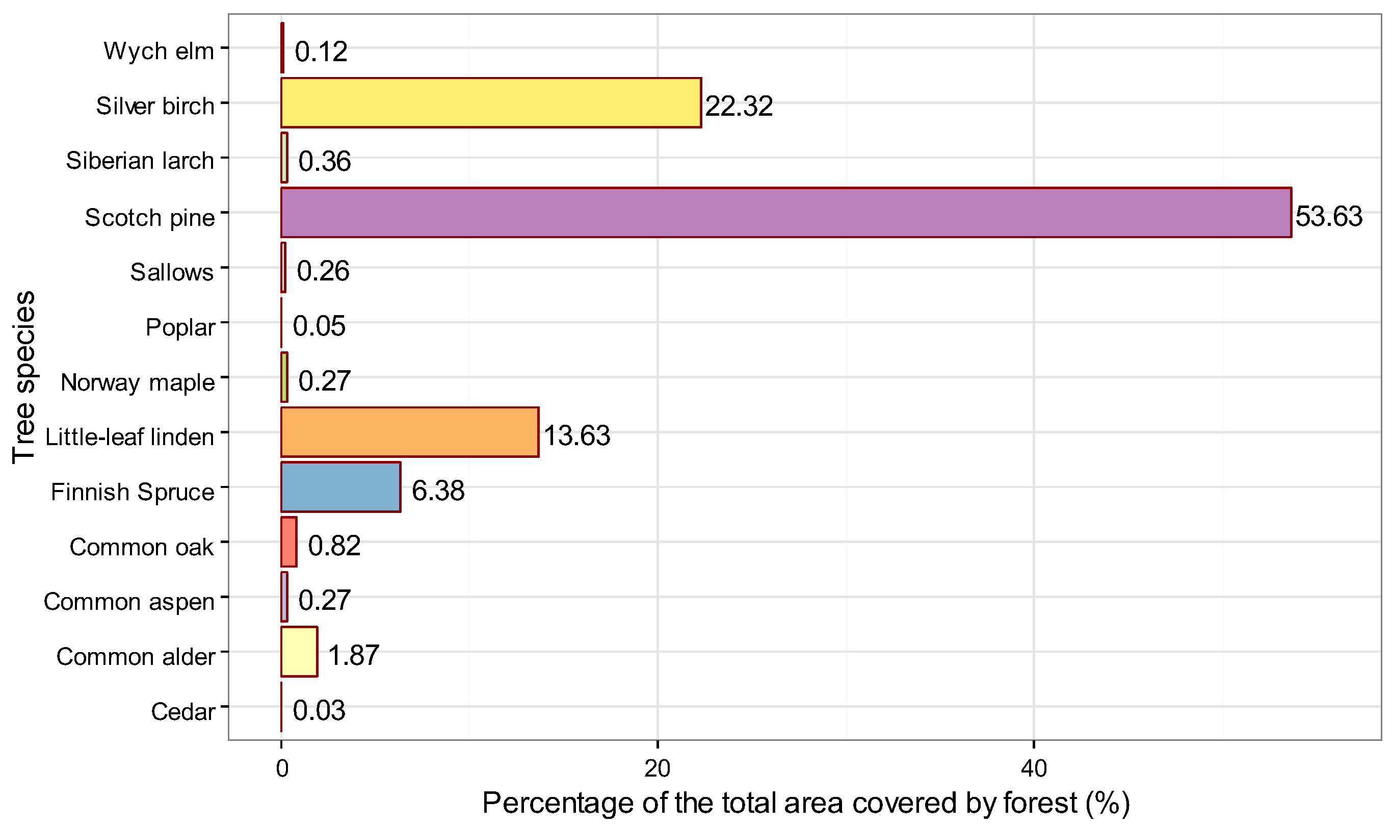
| Tree Species | Number of Stands Where the Species Is Present | Number of Stands with 100% Presence of the Species |
|---|---|---|
| Wych elm (Ulmus glabra Huds.) | 17 | 0 |
| Silver birch (Betula pendula Roth., B. pubescens Ehrh) | 1171 | 69 |
| Siberian larch (Larix sibirica Ledeb.) | 18 | 2 |
| Scotch pine (Pinus sylvestris L.) | 1416 | 375 |
| Sallows (Salix sp.) | 13 | 3 |
| Poplar (Populus sp.) | 5 | 0 |
| Norway maple (Acer platanoides L.) | 33 | 0 |
| Little-leaf linden (Tilia cordata Mill.) | 609 | 8 |
| Finnish spruce (Picea x fennica (Redel) Kom.) | 719 | 1 |
| Common oak (Quercus robur L.) | 74 | 2 |
| Common aspen (Populus tremula L.) | 22 | 1 |
| Common alder (Alnus glutinosa (L.) Gaertn.) | 74 | 4 |
| Cedar (Cedrus sp.) | 3 | 0 |
| File Name | Date | 10 m Bands | 20 m Bands | Cloud Coverage for Study Area | Processing Level |
|---|---|---|---|---|---|
| S2A_MSIL2A_20200509T075611_N0214_R035_T39VUC_20200509T111003 | 2020.05.09 | 2,3,4,8 | 5,6,7,8A,11,12 | 0 | L2A |
| S2A_MSIL2A_20200621T080611_N0214_R078_T39VUC_20200621T112622 | 2020.06.21 | 2,3,4,8 | 5,6,7,8A,11,12 | 0 | L2A |
| S2A_MSIL2A_20200708T075611_N0214_R035_T39VUC_20200708T111246 | 2020.07.08 | 2,3,4,8 | 5,6,7,8A,11,12 | 0 | L2A |
| S2B_MSIL2A_20200805T080609_N0214_R078_T39VUC_20200805T105558 | 2020.08.05 | 2,3,4,8 | 5,6,7,8A,11,12 | 0 | L2A |
| S2B_MSIL2A_20200924T080649_N0214_R078_T39VUC_20200924T102247 | 2020.09.24 | 2,3,4,8 | 5,6,7,8A,11,12 | 0 | L2A |
| S2A_MSIL2A_20201029T081051_N0214_R078_T39VUC_20201029T104651 | 2020.10.29 | 2,3,4,8 | 5,6,7,8A,11,12 | 0 | L2A |
| Tree Species | Short Name | Number of Stands in the Training Sample | Total Area of Stands (ha) in the Training Sample | Number of Stands in the Test Sample | Total Area of Stands (ha) in the Test Sample |
|---|---|---|---|---|---|
| Common alder (Alnus glutinosa (L.) Gaertn.) | alder | 16 | 21 | - | - |
| Finnish spruce (Picea x fennica (Redel) Kom.) | spruce | 11 | 7 | - | - |
| Little-leaf linden (Tilia cordata Mill.) | linden | 17 | 30 | - | - |
| Silver birch (Betula pendula Roth.) | birch | 27 | 26 | 42 | 28 |
| Scotch pine (Pinus sylvestris L.) | pine o. | 24 | 98 | 137 | 316 |
| Old-growth natural forest/stands | |||||
| Scotch pine (Pinus sylvestris L.) | pine y. | 27 | 48 | 116 | 146 |
| Pine plantations on at the felling site | |||||
| Total: | 122 | 230 | 295 | 490 |
| Band | May | June | July | August | September | October |
|---|---|---|---|---|---|---|
| Band 2—Blue | 0.5 | 0.5 | 0.5 | 0.5 | 0.5 | 0.5 |
| Band 3—Green | 0.6 | 0.6 | 0.6 | 0.6 | 0.6 | 0.6 |
| Band 4—Red | 0.5 | 0.5 | 0.5 | 0.5 | 0.6 | 0.8 |
| Band 5— Red-edge I | 0.8 | 0.6 | 0.6 | 0.6 | 1.0 | 0.8 |
| Band 6— Red-edge II | 0.9 | 1.0 | 1.0 | 1.0 | 1.0 | 1.0 |
| Band 7— Red-edge III | 0.9 | 1.0 | 1.0 | 1.0 | 1.0 | 1.0 |
| Band 8—NIR | 0.9 | 1.0 | 1.0 | 1.0 | 1.0 | 1.0 |
| Band 8A—Narrow NIR | 0.9 | 1.0 | 1.0 | 1.0 | 1.0 | 1.0 |
| Band 11—SWIR1 | 0.9 | 0.9 | 0.9 | 0.9 | 0.9 | 1.0 |
| Band 12—SWIR2 | 0.8 | 0.6 | 0.6 | 0.6 | 0.8 | 1.0 |
| NDVI | 0.5 | 0.8 | 1.0 | 1.0 | 0.6 | 0.8 |
| RF/Training Data: | GTM/Training Data: | |||||
|---|---|---|---|---|---|---|
| Tree Species | Recall | Precision | F1-Score | Recall | Precision | F1-Score |
| Alder | 0.977 | 0.988 | 0.983 | 0.665 | 0.563 | 0.610 |
| Spruce | 0.899 | 0.974 | 0.935 | 0.575 | 0.509 | 0.540 |
| Linden | 0.994 | 0.991 | 0.992 | 0.948 | 0.914 | 0.931 |
| Birch | 0.971 | 0.967 | 0.969 | 0.531 | 0.747 | 0.621 |
| pine y. | 0.979 | 0.994 | 0.986 | 0.792 | 0.762 | 0.777 |
| pine o. | 0.998 | 0.988 | 0.993 | 0.891 | 0.895 | 0.893 |
| macro avg | 0.970 | 0.983 | 0.976 | 0.734 | 0.732 | 0.729 |
| accuracy | 0.987 | 0.829 | ||||
| RF/Test Data: | GTM/Test Data: | |||||
| Tree Species | Recall | Precision | F1-score | Recall | Precision | F1-score |
| Birch | 0.694 | 0.606 | 0.647 | 0.546 | 0.600 | 0.572 |
| pine y. | 0.607 | 0.706 | 0.652 | 0.635 | 0.523 | 0.574 |
| pine o. | 0.849 | 0.805 | 0.826 | 0.701 | 0.779 | 0.738 |
| macro avg | 0.717 | 0.706 | 0.709 | 0.628 | 0.634 | 0.628 |
| accuracy | 0.764 | 0.673 | ||||
| Tree Species | Mean of Real Percent | Mean of Model Percent | ME | MAE | RMSE | WAPE | Pearson Correlation Coefficient |
|---|---|---|---|---|---|---|---|
| RF Model | |||||||
| Alder | 1.9 | 5.2 | −3.4 | 4.1 | 10.3 | 2.23 | 0.70 |
| Spruce | 6.3 | 4.5 | 1.8 | 7.0 | 12.6 | 1.10 | 0.39 |
| Linden | 13.6 | 13.1 | 0.5 | 7.1 | 15.2 | 0.52 | 0.83 |
| Birch | 22.2 | 19.4 | 2.8 | 14.3 | 22.7 | 0.64 | 0.68 |
| Pine | 53.4 | 57.8 | −4.4 | 13.8 | 22.9 | 0.26 | 0.86 |
| GTM Model | |||||||
| Alder | 1.9 | 7.1 | −5.3 | 6.6 | 14.9 | 3.56 | 0.45 |
| Spruce | 6.3 | 11.5 | −5.2 | 11.9 | 19.8 | 1.88 | 0.21 |
| Linden | 13.6 | 13.8 | −0.2 | 8.0 | 17.2 | 0.59 | 0.81 |
| Birch | 22.2 | 10.2 | 12.0 | 16.8 | 27.0 | 0.76 | 0.60 |
| Pine | 53.4 | 57.3 | −3.9 | 14.1 | 23.4 | 0.27 | 0.85 |
Disclaimer/Publisher’s Note: The statements, opinions and data contained in all publications are solely those of the individual author(s) and contributor(s) and not of MDPI and/or the editor(s). MDPI and/or the editor(s) disclaim responsibility for any injury to people or property resulting from any ideas, methods, instructions or products referred to in the content. |
© 2023 by the authors. Licensee MDPI, Basel, Switzerland. This article is an open access article distributed under the terms and conditions of the Creative Commons Attribution (CC BY) license (https://creativecommons.org/licenses/by/4.0/).
Share and Cite
Polyakova, A.; Mukharamova, S.; Yermolaev, O.; Shaykhutdinova, G. Automated Recognition of Tree Species Composition of Forest Communities Using Sentinel-2 Satellite Data. Remote Sens. 2023, 15, 329. https://doi.org/10.3390/rs15020329
Polyakova A, Mukharamova S, Yermolaev O, Shaykhutdinova G. Automated Recognition of Tree Species Composition of Forest Communities Using Sentinel-2 Satellite Data. Remote Sensing. 2023; 15(2):329. https://doi.org/10.3390/rs15020329
Chicago/Turabian StylePolyakova, Alika, Svetlana Mukharamova, Oleg Yermolaev, and Galiya Shaykhutdinova. 2023. "Automated Recognition of Tree Species Composition of Forest Communities Using Sentinel-2 Satellite Data" Remote Sensing 15, no. 2: 329. https://doi.org/10.3390/rs15020329
APA StylePolyakova, A., Mukharamova, S., Yermolaev, O., & Shaykhutdinova, G. (2023). Automated Recognition of Tree Species Composition of Forest Communities Using Sentinel-2 Satellite Data. Remote Sensing, 15(2), 329. https://doi.org/10.3390/rs15020329