Scene Classification Based on Heterogeneous Features of Multi-Source Data

Abstract

Remote sensing scene classification is quite important in earth observation and other fields. Previous research has found that most of the existing models are based on deep learning models. However, the classification accuracy of the deep learning model is difficult to break through due to the challenges of difficulty distinguishing the socio-economic attributes of scenes, high interclass similarity, and large intraclass differences. To tackle the challenges, we propose a novel scene classification model that integrates heterogeneous features of multi-source data. Firstly, a multi-granularity feature learning module is designed, which can conduct uniform grid sampling of images to learn multi-granularity features. In this module, in addition to the features of our previous research, we also supplemented the socio-economic semantic features of the scene, and attention-based pooling is introduced to achieve different levels of representation of images. Then, to reduce the dimension of the feature, we adopt the feature-level fusion method. Next, the maxout-based module is designed to fuse the features of different granularity and extract the most distinguishing second-order latent ontology essence features. The weighted adaptive fusion method is used to fuse all the features. Finally, the Lie Group Fisher algorithm is used for scene classification. Extensive experimentation and evaluations show that our proposed model can find better solutions to the above challenges.

1. Introduction

Remote sensing scene classification is the most fundamental research in the field of earth observation, which classifies remote sensing images into different semantic scenes [1]. Scene classification has attracted more and more scholars’ attention and has been widely used in natural hazard detection [2], geospatial object detection [3], and environmental monitoring [4]. Scenes are commonly used to identify accurate urban land-use classification [5]. For example, urban land-use map [6] is drawn based on a high-resolution remote sensing image (HRRSI) scene classification model. Scene classification is also the most challenging research task due to the highly complex socio-economic attributes, geometrical structures, spatial distribution, and various objects inherent in the remote sensing scenes [7].

According to the different levels of features, there are mainly three models [8,9,10,11,12]:

• Traditional approaches design some representative features according to the characteristics of images and the task of classification [13], such as color histograms (CH) [14] and scale-invariant feature transform (SIFT) [15]. The above features are not necessarily independent of one another and some approaches involve two or more features [16].
• This model is designed to accurately capture the complex and changeable features in the scene target object, which is projected into the parameter space or dictionary to learn more effective middle-level features to classify the scene, such as bag-of-visual-words (BoVW) [17]. Later, to solve the problem of high-dimensional feature vector, scholars proposed probabilistic topic model (PTM), such as Latent Dirichlet Allocation model (LDA) [18] and Probabilistic Latent Semantic Analysis (PLSA) [19].
• Classification models based on high-level features: Artificial intelligence and computer vision technologies represented by deep learning (such as convolutional neural network (CNN) [20]) further improve the accuracy of remote sensing image scene classification [8,9,21,22]. In the high spatial remote sensing image scene classification, Xu et al. [9] proposed a novel lightweight and robust Lie Group and CNN joint representation scene classification model, which improved the classification accuracy. Xu et al. [12] proposed a Lie Group spatial attention mechanism to complete high spatial remote sensing image scene classification.

However, the features in the three models are often used interchangeably. Since a certain feature is mainly represented from one aspect, ignoring the feature information from other aspects, to better represent the scene, different features are usually fused, and the feature fusion method has been proven to be effective [23]. Feature fusion is not to add features with the same or similar attributes, but to supplement complementary feature information [8,9]. R. N. Marandi and H. Ghassemian [24] proposed a joint feature representation model. S. Jia. and J. Xian [25] proposed a multitask sparse logistic regression method based on a multi-feature and decision fusion approach for scene classification. Z. Zheng and J. Cao [26] jointly used the low-level features extracted by Ridgelet and the high-level features extracted by CNN to propose the multi-resolution CNN framework. The above models have achieved satisfactory classification results. Theoretically, the more features, the better scenario classification. However, under the constraint of a limited training sample set, too many features will increase the computational space, improve the computational complexity, and easily introduce redundant features. In addition, many scholars have proposed to depict scenes based on multi-source remote sensing data [27,28]. The multi-source remote sensing data in the above studies are mainly from HRRSI, very-high-resolution (VHR) optical images, synthetic aperture radar images, and common standard remote sensing image datasets. However, the above feature fusion methods simply superimpose features without fully considering the relationship and redundancy of features.

The three primary challenges mentioned above are mainly resolved in this study:

1.

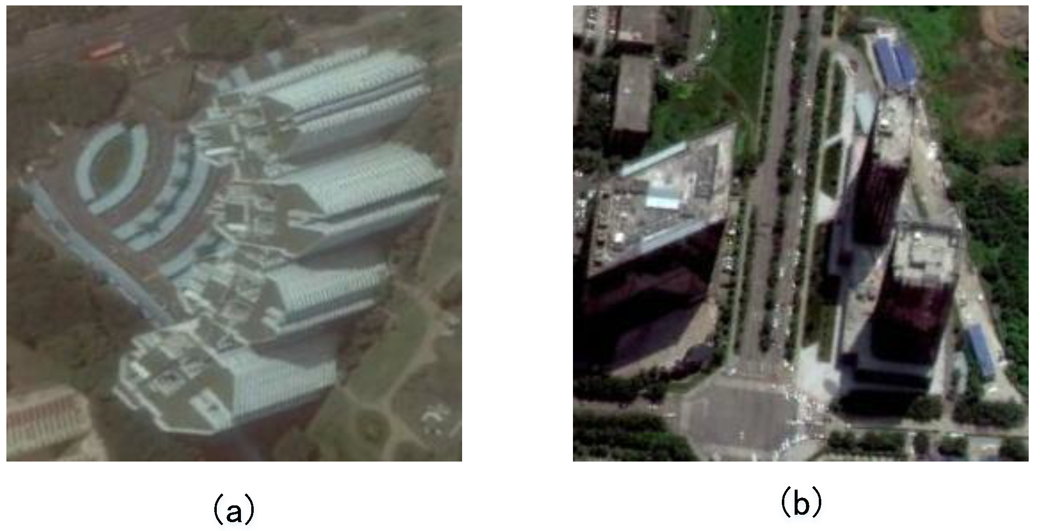
How to distinguish the socio-economic attributes of scenes with the same or similar spatial layouts. The different socio-economic attributes are difficult to express in HRRSI. As shown in Figure 1, the two land parcels in the scenario have several office buildings, one of which are enterprise, while the other is a government agency. It is hard to differentiate the one from the other.

2.

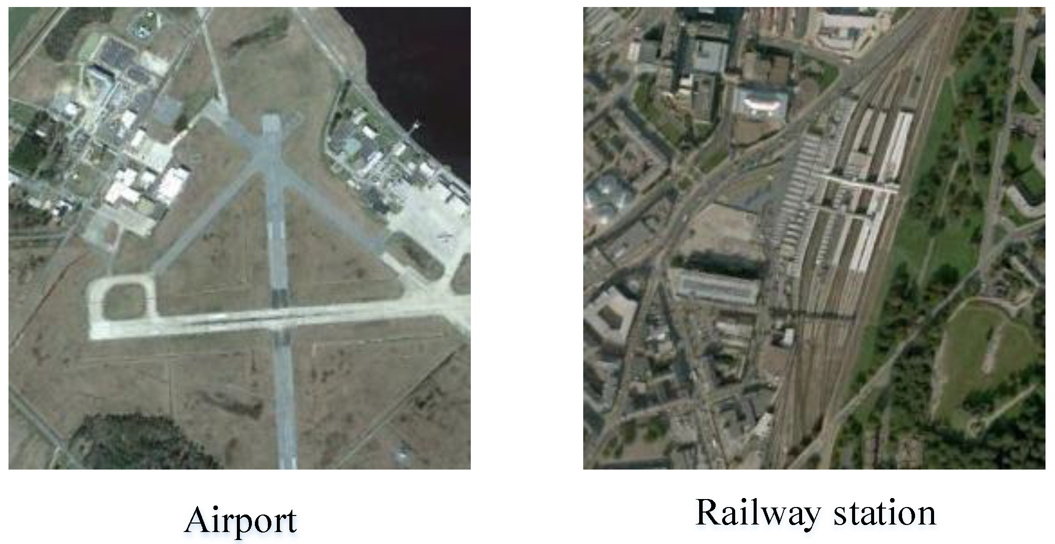
How to solve the visual-semantic differences caused by the matching between the features learned by the model and the corresponding semantic categories. As shown in Figure 2, an airport scenario consists of airplanes and runways, a railway scenario consists of railway stations and railways, and a bridge may belong to freeways. These three categories can be regarded as three layers: the first layer (i.e., transportation), the second layer (i.e., airports, bridges, and railways), and the third layer (i.e., runways) [29]. The second and third layers are easier to classify, while the first layer requires more discriminative features. However, most of the existing models can learn high-level features [30], but they cannot be well integrated with high-level semantics well into category labels [31].

3.

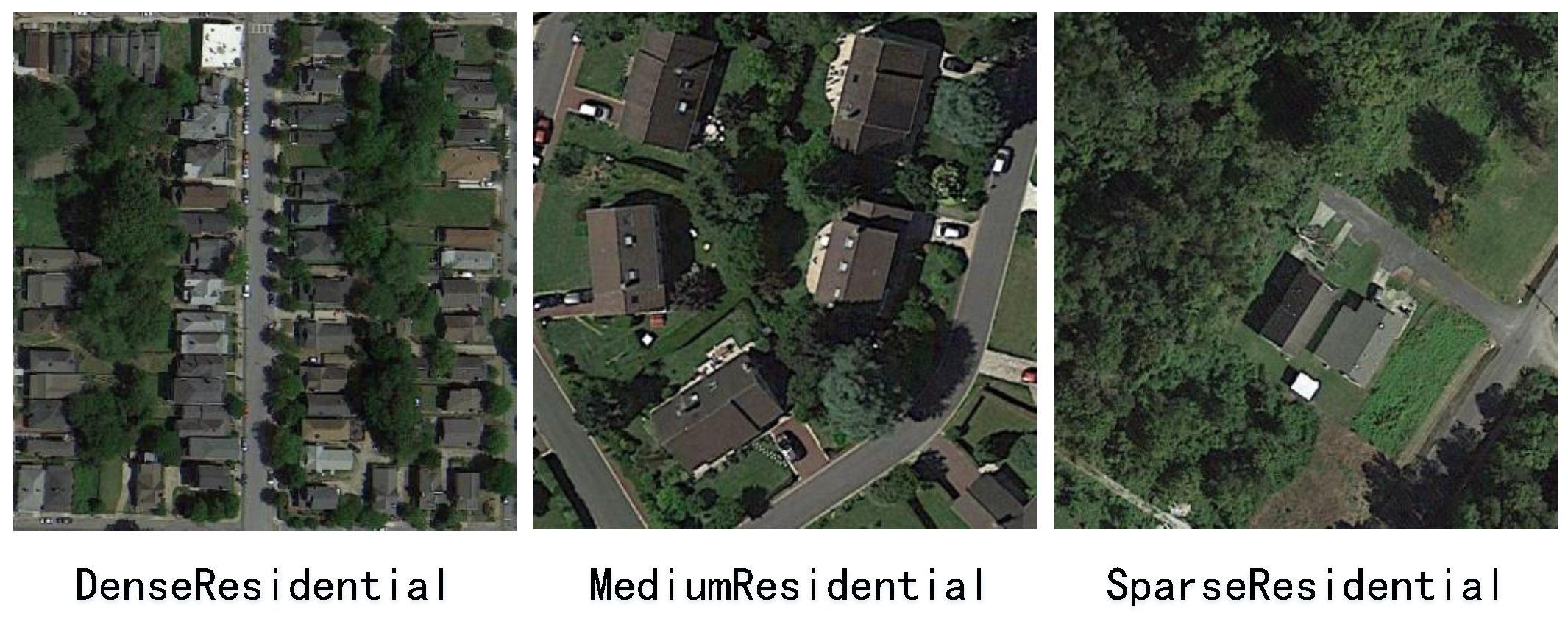
How to resolve low between-class separability (also known as high interclass similarity). As shown in Figure 3, dense residential, medium residential, and sparse residential all contain the same two modalities (houses and trees). These categories have high intraclass similarities. Most of the existing models ignore the diversity between classes and higher intraclass similarity of the scene, most of the existing models are mainly applied to the scene classification dominated by single-modality-dominated scenes, which has limitations when encountering multimodality-dominated scenes.

To tackle the above challenges, we propose a novel scene classification model based on point-line-surface multi-source heterogeneous features. To address the first challenge, the model not only extracted the external physical structure features (i.e., structure and texture) of the scene but also supplements the inner socio-economic semantics to enhance the ability of scene feature representation. To address the second challenge, the image is sampled by a multi-scale grid for multi-grained feature learning, and the trainable pooling layer of an attention mechanism is introduced to highlight the local semantics relevant to the scene category labels and reduce the visual-semantic discrepancies. To address the third challenge, the multi-level supervision strategy is introduced, the weighted adaptive fusion approach is used to fuse the multi-scale sampling granularity and focus on the basic-level or superordinate-level intraclass diversity, and the Lie Group Fisher scene classification algorithm is used to achieve intra-class minimization and inter-classes maximization.

The primary contributions of this study are as follows:

• To solve the problem of scenes with the same or similar spatial layout, but with different socio-economic attributes. We propose a classification model based on heterogeneous characteristics of multi-source data. This model makes full use of the heterogeneous characteristics of multi-source data, including the external physical structure features in previous studies and the internal socio-economic semantic features of the scene, enriching the features of the scene.
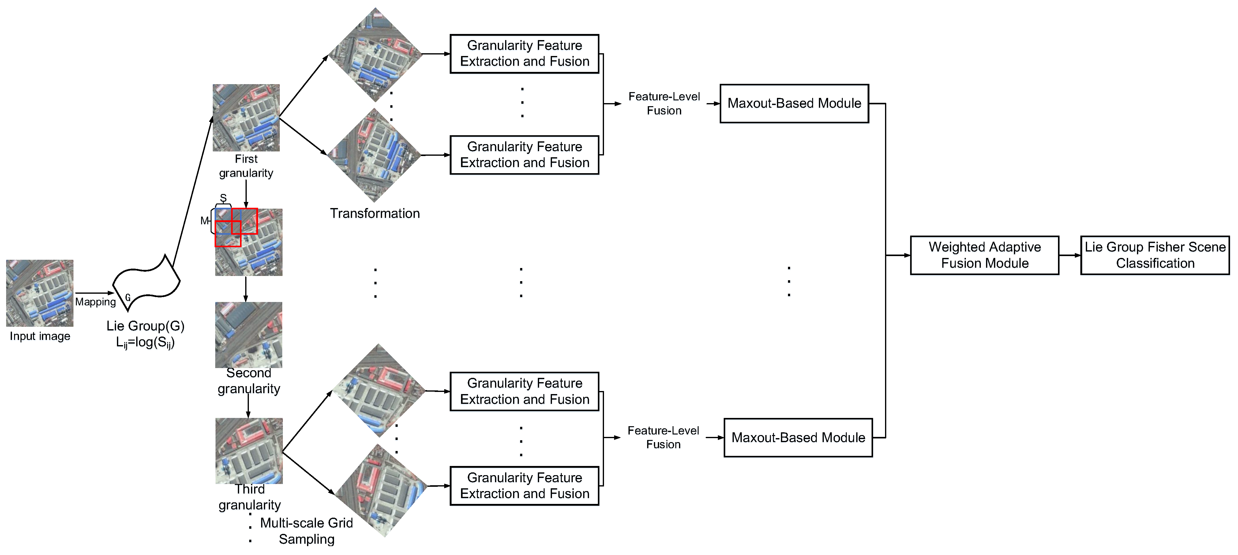
• To resolve the problem of visual-semantic discrepancies, in our proposed model, multi-scale grid sampling is carried out on HRRSI to learn different degrees of multigrained features, and the attention mechanism is introduced. The Lie Group covariance matrix with different granularity is constructed based on the maxout module to extract the second-order features of the latent ontological essence of the HRRSI.
• To resolve the problem of the high interclass similarity, the weighted adaptive fusion module is adopted in our proposed model to fuse the features extracted from different granularity, and a Lie Group Fisher scene classification algorithm is proposed. By calculating the intrinsic mean of the fused Lie Group features of each category, a geodesic is found in the Lie Group manifold space, and the samples are mapped to the geodesic, minimizing intra-class and maximizing inter-class.

2. Materials and Methods

The core idea of our proposed model is hierarchical extraction and learning of multi-granularity and multi-source heterogeneous features, enhancing scene representation ability and reducing visual-semantic discrepancies, fusing multi-granularity features, and introducing attention mechanism to extract latent ontology features. As shown in Figure 4. Specifically: (1) Map the data to the Lie Group manifold space (LGMS) and obtain the Lie Group data; (2) multi-scale grid sampling of Lie Group data samples; (3) a granularity feature extraction and fusion module is designed, which can learn multi-source heterogeneous features with different granularity with the help of multi-source geospatial data and attention mechanism; (4) extract the most distinguishing second-order feature of potential ontology essence in HRRSI, and design a Lie Group regional covariance heterogeneous feature matrix based on max-out multi-source data; (5) a Lie Group Fisher scene classification algorithm is designed for classification.

2.1. Sample Mapping

According to the previous research [8,9,10,11], firstly, we map the samples to the LGMS to obtain the Lie Group samples:

$${\mathbf{L}}_{ij}=log\left(S_{ij}\right)$$

(1)

where $S_{ij}$ represents the $j^{th}$ sample of the $i^{th}$ class in the data set, and ${\mathbf{L}}_{ij}$ represents the $j^{th}$ sample of the $i^{th}$ class in the manifold space of the Lie Group. The following operations are based on the Lie Group data sample ${\mathbf{L}}_{ij}$.

2.2. Multi-Scale Grid Sampling

Previous researchers have shown that uniform grid sampling and image decomposition can improve scene representation [9,33]. For the Lie Group data sample ${\mathbf{L}}_{ij}$, firstly, the entire sample is taken as the first granularity ${\mathbf{g}}_{ij}$. Then, the whole sample ${\mathbf{L}}_{ij}$ is uniformly grid sampled by the patch size M and spacing S. The generated patches were then matched to a sub-region based on the maximum overlap region. Multi-scale sampling was performed for each patch. The center of the initial patch is $(x_0,y_0)$, and the size is $r_0\times r_0$. Subsequent granularity was constructed continuously until the size reaches the maximum of the image. After multi-scale grid sampling, the next granularity ${\mathbf{g}}_{i+1,j+1}$ is obtained. Figure 5 shows the multi-scale grid sampling method. To avoid feature variance, the rotation transformation is performed for each granularity [31].

$${\mathbf{g}}_{ij}^t=\psi \left({\mathbf{g}}_{ij}\right)$$

(2)

where, ${\mathbf{g}}_{ij}^t$ represents the $t^{th}$ transition state of the granularity of the $j^{th}$ sample of the $i^{th}$ category, $\psi (·)$ represents the rotation function.

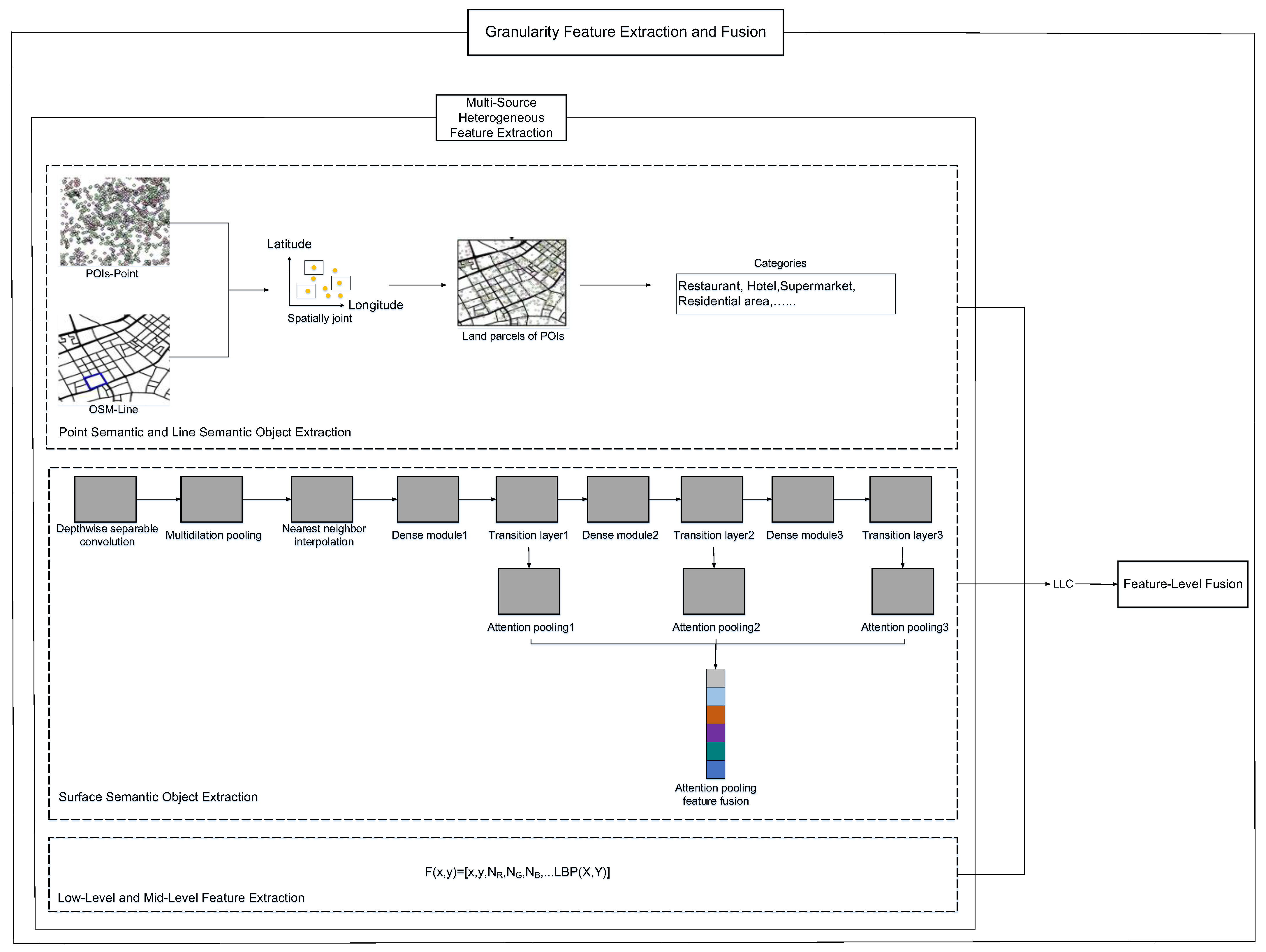
2.3. Granularity Feature Extraction and Fusion

Since we need to extract, learn, and fuse the features of the most distinguished transformed images in scene classification, a granularity feature extraction, and fusion module is designed to learn features, as shown in Figure 6.

2.3.1. Multi-Source Heterogeneous Feature Extraction

To effectively extract the socio-economic semantics features of the scene, inspired by [34], this study makes full use of multi-source geospatial data in diverse formats, such as volunteered geographic information (VGI) data and social media data, to reflect the real situation of the scene from different aspects.

Point Semantic Object Extraction The scene usually contains several points of interest (POI), OpenStreetMap (OSM) boundary lines, and surface (polygon) semantic objects. In general, the objects in the scene can be modeled as points (or pixels), lines, and surfaces (polygonal) [35], which are widely used because they contain information such as category and position [36].

In this section, the semantic features of the main categories are extracted from Amap. POI can effectively represent local detail features and contain socio-economic semantics.

Line Semantic Object Extraction Scholars usually utilized OSM polygon data to represent the ground-truth data [37], and also utilized road network data to represent the boundary of the scene land parcel [38]. To effectively improve the accuracy of geo-referencing and the quality of data, in the design and implementation process of the algorithm, we first reprojected point-line-surface (polygon) data into the WGS_1984_World_Mercator system, and corrected the topology errors of OSM line data, and utilized OSM line data to determine the scene boundary. Then, longitude and latitude are used to spatially associate POIs with the scene.

Surface semantic object extraction In this section, an attention mechanism is used for the extraction of surface semantic objects, in which the pooling layer is used to highlight local semantic information related to scene categories, as shown in Figure 6.

① Convolution Layer Module: To improve the calculation speed and reduce the amount of calculation, we continue the previous approach [9,39] and utilized $3\times 3$ depthwise separable convolution.

② Multidilation Pooling Module: To learn higher-level abstract features and achieve multi-scale feature representation, the previous research approach [9] is adopted in the model, and the multidilation pooling module is utilized. For details, please refer to our previous research [9].

③ The Nearest Neighbor Interpolation Module: Since the features extracted by the above multidilation pooling modules are different in size, to effectively improve the ability of feature representation, we utilized the nearest neighbor interpolation method to upsample the extracted feature maps and convert them into the same size dimensions. Furthermore, to extract deeper convolution features, the feature maps are longitudinally fused, and the pyramid and deep convolution features are extracted.

④ Dense Module: This module contains composition functions and the corresponding connections, as shown in Figure 7, let $l_{i-1}$ and $l_i$ represent the output of the ${i-1}^{th}$ and the $i^{th}$ layer, respectively, $C(·)$ represents the composition function at the $i^{th}$ layer, and the relationship between $l_i$ and $l_{i-1}$ is represented by:

$$l_i=C_i\left(l_{i-1}\right)$$

(3)

$$l_i=C_i\left([l_0,l_1,\cdots ,l_{i-1}]\right)$$

(4)

The composite function is represented by $BN$-$ReLU$-$Conv1$-$BN$-$ReLU$-$Conv3$, where $BN$ represents batch normalization operation, $ReLU$ represents activation function, $Conv1$ represents $1\times 1$ convolutional layer and $Conv3$ represents $3\times 3$ convolutional layer.

⑤ Transition Layer: This layer is mainly composed of a $1\times 1$ average pooling and convolution layer, which is mainly to change the channel number of feature map and down-sampling operation.

⑥ Attention Pooling Module: f represents the feature map from the transitional layer, ${\mathbf{f}}_{ij}$ represent the feature vector of ${\mathbf{f}}_{ij}$ in pixel $(i,j)$, and the attention weight $w_{ij}$ is calculated as follows:

$$\left\{w_{ij}\right\}=softmax\left(ReLU({\mathbf{W}}_1{\mathbf{f}}_{ij}^T+\mathbf{b})\right)$$

(5)

where $softmax$ represents the softmax operation, $ReLU$ represents the activation function, ${\mathbf{W}}_1$ represents the trainable weight parameter matrix, and b represents the bias matrix.

Let ${\mathbf{f}}_{ij}$ represents the gray value at the pixel position $(i,j)$, and S represents the window size of the pooling operation. After using the mean pooling, the gray value ${\mathbf{f}}^{\prime }$ of the corresponding pixel is as follow:

$${\mathbf{f}}^{\prime }=\frac{{\sum }_{m=0,n=0}^S\mathbf{f}(i+m,j+n)}{S\times S}$$

(6)

In contrast, ${\mathbf{f}}^{\prime }$ is obtained by utilizing attention-based pooling:

$$textbf{f}^{\prime }=\frac{{\sum }_{m=0,n=0}^S{w}_{i+m,i+n}\mathbf{f}(i+m,j+n)}{S\times S}$$

(7)

The pooling operation of the attention mechanism can make up for the loss of local feature information caused by the use of weight sharing in the existing CNN model, assign higher weights to the important local features in the image, and also complete the operation of down-sampling the features. The generation process of attention weight is shown in Figure 8.

⑦ Multi-Level Supervision Strategy: The current deep supervision strategies are usually supervised after feature extraction or fusion because it is impossible to directly generate category prediction in shallower features [40]. In our model, a multi-level supervision strategy is used to supervise the training process.

Low-Level and Mid-Level Feature Extraction The core issue of scene classification is to bridge the gap between raw visual features and target semantics through feature representation or coding. Recent studies have demonstrated that the fusion of low-level and mid-level features (such as spatial structure features) can make features more discriminating [41]. To further improve the ability to represent complex scenes, based on the above point-line-surface multi-source heterogeneous feature extraction, we further extracted the low-level and mid-level features of the scene, as shown below:

$$F(x,y)=[x,y,N_R,N_G,N_B,Y,C_b,C_r,\left|\frac{\partial I(x,y)}{\partial x}\right|,\left|\frac{\partial I(x,y)}{\partial y}\right|,\left|\frac{{\partial }^{2}I(x,y)}{\partial x^2}\right|,\left|\frac{{\partial }^{2}I(x,y)}{\partial y^2}\right|,$$

(8)

$$Gabor(x,y),SIFT(x,y){]}^T$$

where the above features include gradient, pixel position, LBP, and other features. The specific meaning of the formula can be referred to in our previous research [9].

Finally, an effective and simple locality-constrained linear coding(LLC) technique is used to address the gap between visual semantics and high-level semantics.

2.3.2. Feature-Level Fusion

Multi-source heterogeneous features have their meanings and properties. To better improve the ability of feature characterization, this section adopted discriminant correlation analysis (DCA) to fuse multi-source heterogeneous features [42].

Assume that the heterogeneous feature dataset $H{f}_1$, its n columns are divided into C classes, $n_i$ represents the corresponding class of $i^{th}$, ${\mathbf{hf}}_{i,j}$ represents the feature vector of the $j^{th}$ sample of the $i^{th}$ class. Firstly, calculate the divergence inter-class:

$$S_{ic}=\sum _{i=1}^C{n}_i({\overline{x}}_i-\overline{x}){({\overline{x}}_i-\overline{x})}^T={\Psi }_{ic}{\Psi }_{ic}^T$$

(9)

where, ${\overline{x}}_i$ represents the intrinsic mean of Lie Group of the $i^{th}$ class, and $\overline{x}$ represents the intrinsic mean in the Lie Group of the whole feature set. The calculation of the intrinsic mean in Lie Group can refer to our previous research [10,11].

Then, the eigenvectors of ${\Psi }_{ic}{\Psi }_{ic}^T$ are calculated. The dimension of $H{f}_1$ can be effectively reduced, and $H{f}_1$ is projected in low-dimensional space:

$$H{f}_1^{\prime }=U_{ic}^{T}H{f}_1$$

(10)

where $U_{ic}$ represents the transformation using $S_{ic}$, and different categories are easier to distinguish in lower-dimensional space. To facilitate understanding, this section takes two heterogeneous features as examples. Given another type of heterogeneous feature data sets $H{f}_2$, the relevant $H{f}_2^{\prime }$ can be obtained by the above method.

Then, $H{f}_1^{\prime }$ and $H{f}_2^{\prime }$ are transformed so that there is a nonzero correlation between them:

$${\breve{Hf}}_1=U_{c{c}_1}^{T}H{f}_1^{\prime }$$

(11)

$${\breve{Hf}}_2=U_{c{c}_2}^{T}H{f}_2^{\prime }$$

(12)

where $U_{c{c}_1}$ and $U_{c{c}_2}$ use $S_{c{c}_1}^{\prime }=H{f}_1^{\prime }{H{f}_2^{\prime }}^T$.

Finally, the transformed feature vectors are obtained by concatenating:

$$F{u}_{s_{1,2}}={\left({\breve{Hf}}_1,{\breve{Hf}}_2\right)}^T$$

(13)

Compared with the raw features, the above fused features have a stronger representational ability, and the dimensions of the fused features are effectively reduced.

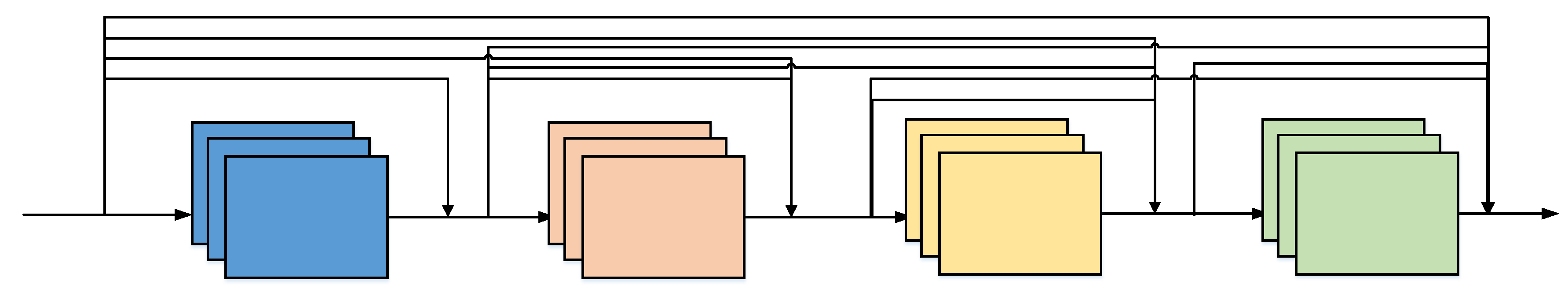
2.4. Maxout-Based Module

To further extract the optimal second-order features and the most discriminating features of ontology essence in the HRRSI, inspired by [43], the maxout-based module is used to extract the above features in this section, and learn the covariance matrices of feature Lie Groups with different granularity corresponding to the features, as shown in Figure 9. The module can solve the problem of intraclass variations in multi-transformations to a certain extent.

In the actual design of the model, before the maxout processing operation, the fused heterogeneous features are first transformed into the feature Lie Group covariance matrices. The traditional deep learning feature is commonly first-order, while the feature Lie Group covariance matrices are second-order, which retains more spatial correlation information under the same granularity. The feature covariance matrix is expressed as:

$${\mathbf{C}}_i^t=\frac{1}{n^2-1}\sum _{k=1}^n\sum _{k=1}^n({\mathbf{z}}_k-\mu ){({\mathbf{z}}_k-\mu )}^T$$

(14)

where $\mu$ represents the intrinsic mean of the regional feature points, other relevant contents can be referred to in our previous research [9].

Inspired by [44], the Gaussian model is constructed by using feature Lie Group covariance matrix:

$${\mathbf{G}}_i^t=\left[\begin{array}{cc}{\mathbf{C}}_i^t+\overline{f}{\overline{f}}^T& \overline{f}\\ {\overline{f}}^T& 1\end{array}\right]$$

(15)

where $\overline{f}={\sum }_{n=1}^N{\mathbf{f}}_n$, the ${\mathbf{G}}_i^t$ matrix obtained is located on the Lie Group manifold space. In previous research, we found that Euclidean space is not closed when negative scalar multiplication is used [8]. In addition, the matrix obtained above is not located in Euclidean space, but in the Lie Group manifold space. As shown in Figure 10, (a) represents the manifold distance, the distance between two data points in the manifold space is located in the manifold space; (b) directly uses the Euclidean distance to calculate the distance between two data points, which is not in the manifold space. The advantage of Lie Group manifold space distance is that it can better and more truly represent the actual distance between two data points, to distinguish different data samples more effectively. Therefore, to better measure distance, we choose the Lie Group manifold space distance instead of Euclidean space distance, and flatten it into a spatial structure by logarithmic operation, as shown below:

$${\check{\mathbf{G}}}_i^t={\mathbf{G}}_i^t+trace\left({\mathbf{G}}_i^t\right){\mathbf{I}}_G$$

(16)

where ${\mathbf{I}}_G$ represents the identity matrix with the same dimension as ${\mathbf{G}}_i^t$.

${\check{\mathbf{G}}}_i^t$ represents the feature of the $i^{th}$ granularity of the $t^{th}$ transformation of the input image, and the optimal second-order feature of ${\check{\mathbf{G}}}_i^t$ is extracted using the following:

$$Os{f}_i^t=f_{Osf}\left({\check{\mathbf{G}}}_i^t\right)$$

(17)

where, $Os{f}_i^t$ represents the optimal second-order feature of ${\check{\mathbf{G}}}_i^t$, $f_{Osf}(·)$ represents the learning process function, and further, adopt the maximum operator operation to select the most distinguishing feature:

$$Os{f}_i^{to}=\underset{t\in T}{\max }Os{f}_i^t$$

(18)

where $to$ represents the most distinguishing feature among all the optimal second-order features of different transformations.

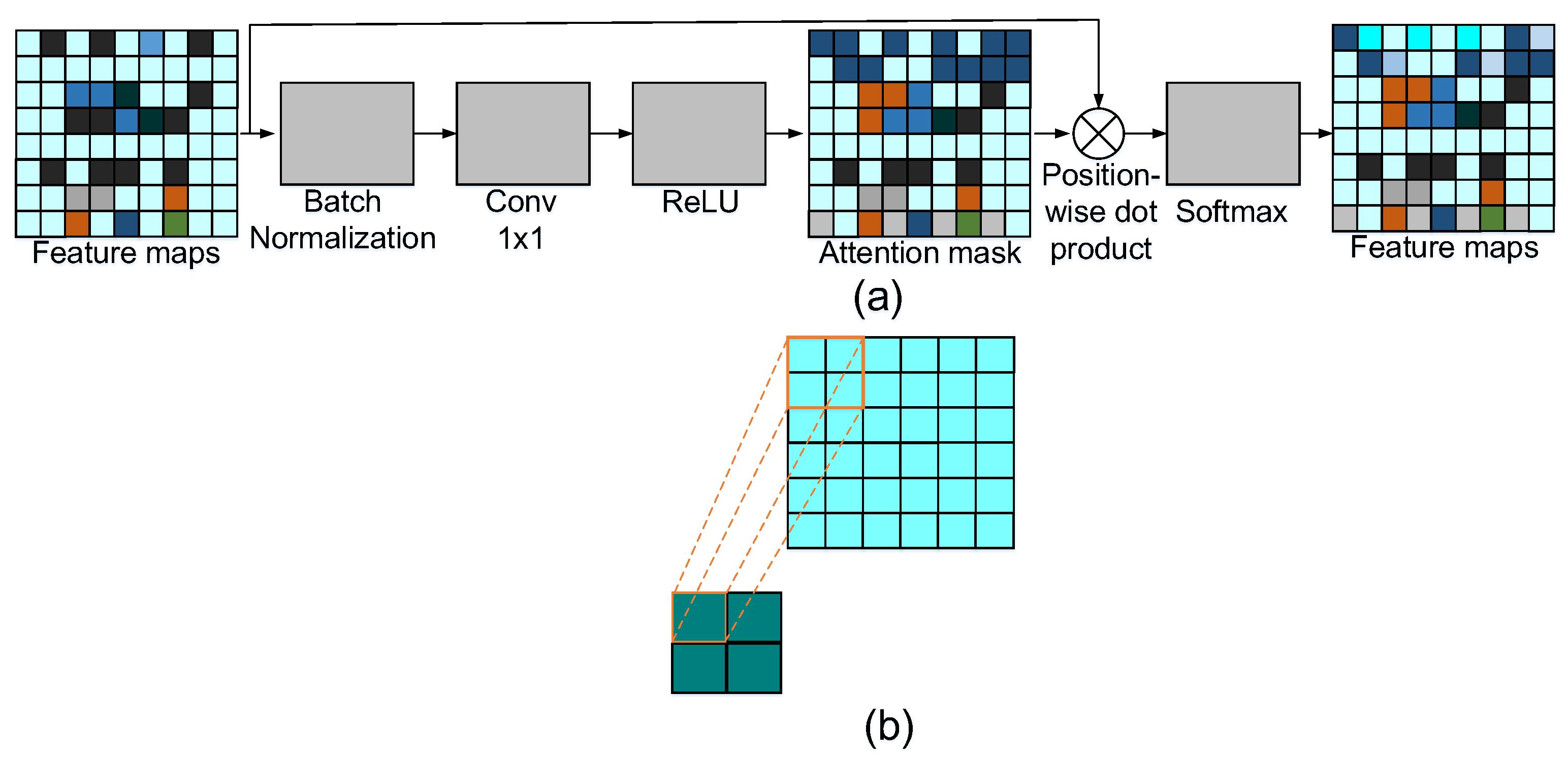
2.5. Weighted Adaptive Fusion Module

Since the image sample data is evenly decomposed into multiple granularities, a weighted adaptive fusion method needs to be designed to fuse the features extracted from all granularities. The inputs of the adaptive weighted fusion framework are the optimal second-order $Os{f}_i$, in the actual model design, the weight is assigned according to $Os{f}_i$, all the optimal second-order features are expressed as a column vector $\mathbf{Osf}={[Os{f}_1,Os{f}_2,\cdots ,Os{f}_n]}^T$, the size of $n\times 1$. Firstly, the normalization operation is carried out, as follow:

$$\overrightarrow{Osf}=\frac{\mathbf{Osf}}{{\sum }_{n=1}^N\mathbf{Osf}}$$

(19)

Its range is $[0,1]$, and the granularity with larger optimal second-order features can obtain larger weights in the vector $\overrightarrow{Osf}$ to describe its importance.

2.6. Lie Group Fisher Scene Classification

The core of the Fisher Linear Discriminant Analysis (FLDA) algorithm is to project raw data onto a hyperplane with lower dimensions to increase the ratio of intra-class divergence to inter-class divergence [45]. However, such algorithms are mainly applied in Euclidean space and have limitations on data samples in non-Euclidean space, and LGMS belongs to non-Euclidean space. Therefore, in this section, we propose the Lie Group Fisher method, as shown in Figure 11, to find a suitable geodesic on the LGMS, and map the sample of Lie Group to the geodesic to maximize the intra-class divergence and inter-class divergence.

3. Results

In this section, we discuss the comprehensive experiments and analyses that were carried out to evaluate the feasibility and applicability of our proposed approach.

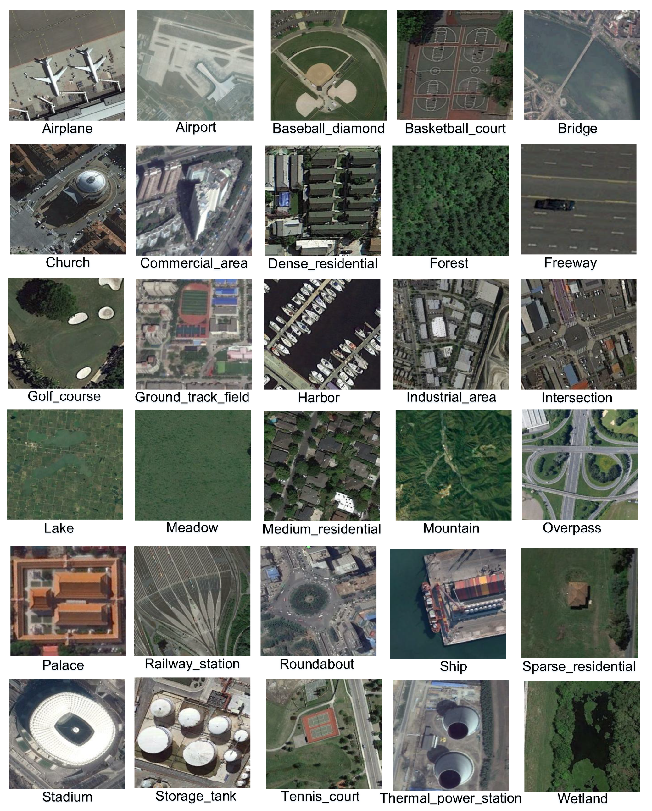
3.1. Experimental Datasets

Since it is impossible to obtain the POI socio-economic semantics and line semantics of OSM data corresponding to UC Merced(UCM) dataset [46], Aerial Images Dataset (AID) [32], and NWPU-RESISC45 dataset [47], to verify the feasibility of our proposed approach, we adopted Google Earth, GF, and other images to make the same or similar scene images with the above three data sets, but there are corresponding POI and OSM data to match them. There are a total of 30 categories, each category has about 60 to 100 images, the spatial resolution of the image is 0.5m to 8m, and the image size is $256\times 256$ pixels to $600\times 600$ pixels. We call this data set the URSIS data set, as shown in Figure 12. Two sets of VGI data were employed in the experiment. The OSM data were obtained on 6 September 2018 (https://www.openstreetmap.org), and the POIs data were obtained from Amap (https://lbs.amap.com/) on 7 October 2018, including longitude, latitude, and category (such as industrial building, hotel).

3.2. Experiment Setup

Since imbalanced data will affect the experiment [48], the samples were set to the same size and quantity in the experiment. Meanwhile, to avoid overfitting, data augmentation techniques are also used to increase the number of data samples. The relevant parameters are set by referring to [49,50], as shown in

Table 1. Experimental environment parameters.

Item	Content
Processor	Inter Core i7-4700 CPU with 2.70 GHz $\times 12$
Memory	64 GB
Operating system	CentOS 7.8 64 bit
Hard disk	1T
GPU	NVIDIA Titan-X $\times 2$
Python	3.7.2
PyTorch	1.4.0
CUDA	10.0
Learning rate	${10}^{-8}$
Momentum	0.9
Weight decay	$5\times {10}^{-4}$
Batch	16
Saturation	1.5
Subdivisions	64

. In this study, overall accuracy (OA), Kappa coefficient, standard deviation (SD), and confusion matrix were selected for evaluation. All experimental evaluations followed the protocol in [32,47]. Ten repeated experiments were conducted to eliminate the contingency of the experiment.

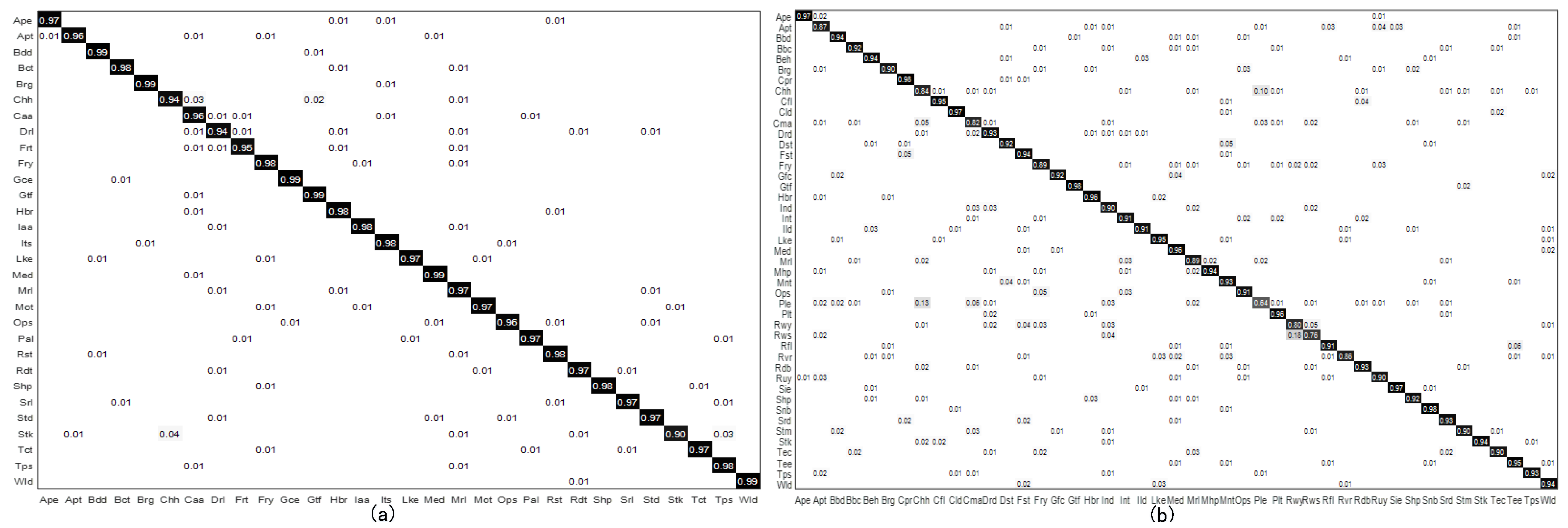
3.3. Experimental Results and Analysis

We selected the fine-tuned AlexNet, GoogLeNet, and other models for comparison, as shown in

Table 2. Overall accuracies(%) of ten kinds of methods and our method under the training ratios of 20% and 50% in URSIS.

Models	Training Ratios
	20%	50%
GIST [47]	$18.63\pm 0.16$	$21.35\pm 0.25$
LBP [47]	$22.37\pm 0.23$	$26.51\pm 0.32$
CH [47]	$29.65\pm 0.15$	$32.87\pm 0.15$
BoVM [47]	$46.95\pm 0.35$	$51.35\pm 0.21$
LLC [47]	$41.66\pm 0.22$	$46.11\pm 0.22$
BoVM+SPM [47]	$35.39\pm 0.17$	$40.16\pm 0.15$
AlexNet [51]	$82.37\pm 0.16$	$85.72\pm 0.54$
GoogLeNet [51]	$78.52\pm 0.16$	$82.13\pm 0.22$
VGG-D [51]	$79.95\pm 0.23$	$83.67\pm 0.12$
MGFN [31]	$93.76\pm 0.22$	$96.32\pm 0.15$
Proposed	$94.86\pm 0.22$	$98.75\pm 0.27$

. Compared with other approaches, the accuracy of the approach based on handcrafted features (i.e., GIST [47], LBP [47], CH [47]) is lower. When the training ratio is 20%, compared with GIST [47] and LBP [47], the accuracy of CH is improved by 11.02% and 7.28%, but it is still lower than 30%. The main reason is that the selection and design of features are based on subjectivity and cannot well represent complex scenes. From the experiment, we found that the accuracy of the handcrafted-based method is low, while the accuracy of the unsupervised feature learning method is high. The deep learning model has great advantages. At the same training ratio (20%), the accuracy of our model is 94.86%, 12.49% higher than AlexNet [51] and 1.1% higher than MGFN [31]. At the same training ratio of 50%, the accuracy of our model is 98.75%, 15.08% higher than VGG-D [51]. Experimental results validate the effectiveness of feature learning in our proposed method.

At the same time, we also selected some of the state-of-the-art representative deep learning models for comparison, as shown in

Table 3. Overall accuracies (%) of twenty-six kinds of methods and our method under the training ratios of 20% and 50% in URSIS.

Models	Training Ratios
	20%	50%
CaffeNet [32]	$86.72\pm 0.45$	$88.91\pm 0.26$
VGG-VD-16 [32]	$85.81\pm 0.25$	$89.36\pm 0.36$
GoogLeNet [32]	$83.27\pm 0.36$	$85.67\pm 0.55$
Fusion by addition [17]	−	$91.79\pm 0.26$
LGRIN [9]	$94.74\pm 0.23$	$97.65\pm 0.25$
TEX-Net-LF [41]	$93.91\pm 0.15$	$95.66\pm 0.17$
DS-SURF-LLC+Mean-Std-LLC+ MO-CLBP-LLC [42]	$94.69\pm 0.22$	$96.57\pm 0.27$
LiG with RBF kernel [11]	$94.32\pm 0.23$	$96.22\pm 0.25$
ADPC-Net [56]	$88.61\pm 0.25$	$92.21\pm 0.26$
VGG19 [57]	$86.83\pm 0.26$	$91.83\pm 0.38$
ResNet50 [57]	$92.44\pm 0.16$	$93.81\pm 0.16$
InceptionV3 [57]	$92.65\pm 0.19$	$94.97\pm 0.22$
DenseNet121 [58]	$92.91\pm 0.25$	$94.65\pm 0.25$
DenseNet169 [58]	$92.39\pm 0.35$	$93.46\pm 0.27$
MobileNet [59]	$87.91\pm 0.16$	$91.23\pm 0.16$
EfficientNet [60]	$87.37\pm 0.16$	$89.41\pm 0.15$
Two-Stream Deep Fusion Framework [61]	$92.42\pm 0.38$	$94.62\pm 0.27$
Fine-tune MobileNet V2 [62]	$94.42\pm 0.25$	$96.11\pm 0.25$
SE-MDPMNet [62]	$93.77\pm 0.16$	$97.23\pm 0.16$
Two-Stage Deep Feature Fusion [63]	−	$93.87\pm 0.35$
Contourlet CNN [55]	−	$96.87\pm 0.42$
LCPP [53]	$91.12\pm 0.35$	$93.35\pm 0.35$
RSNet [30]	$94.62\pm 0.27$	$96.78\pm 0.56$
SPG-GAN [52]	$92.31\pm 0.17$	$94.53\pm 0.38$
TSAN [54]	$89.67\pm 0.23$	$92.16\pm 0.25$
LGDL [8]	$93.97\pm 0.16$	$97.29\pm 0.35$
Proposed	$94.86\pm 0.22$	$98.75\pm 0.27$

. Taking the training ratio of 20% as an example, our proposed model has reached 94.86%, 0.89% higher than LGDL [8], 2.55% higher than SPG-GAN [52], 0.12% higher than LGRIN [9], 3.74% higher than LCPP [53], and 0.24% higher than RSNet [30]. The experimental results show that the classification accuracy has been significantly improved after using the heterogeneous feature of multi-source data, which also shows the importance and necessity of feature learning. The results of the Kappa coefficient are shown in

Table 4. Overall accuracies (%), Kappa coefficient and the standard deviation of twenty-six kinds of methods and our method under the training ratios of 50% in URSIS.

Models	OA (50%)	Kappa (%)	SD
CaffeNet [32]	$88.91$	$86.72$	$0.85$
VGG-VD-16 [32]	$89.36$	$87.24$	$0.82$
GoogLeNet [32]	$85.67$	$83.51$	$0.89$
Fusion by addition [17]	$91.79$	$89.85$	$0.78$
LGRIN [9]	$97.65$	$95.43$	$0.42$
TEX-Net-LF [41]	$95.66$	$94.57$	$0.55$
DS-SURF-LLC+Mean-Std-LLC+MO-CLBP-LLC [42]	$96.57$	$94.39$	$0.47$
LiG with RBF kernel [11]	$96.22$	$95.73$	$0.49$
ADPC-Net [56]	$92.21$	$90.26$	$0.69$
VGG19 [57]	$91.83$	$88.62$	$0.76$
ResNet50 [57]	$93.81$	$92.16$	$0.67$
InceptionV3 [57]	$94.97$	$93.71$	$0.65$
DenseNet121 [58]	$94.56$	$93.83$	$0.66$
DenseNet169 [58]	$93.46$	$92.72$	$0.73$
MobileNet [59]	$91.23$	$89.79$	$0.81$
EfficientNet [60]	$89.41$	$87.53$	$0.82$
Two-Stream Deep Fusion Framework [61]	$94.62$	$93.57$	$0.67$
Fine-tune MobileNet V2 [62]	$96.11$	$94.86$	$0.53$
SE-MDPMNet [62]	$97.23$	$96.15$	$0.46$
Two-Stage Deep Feature Fusion [63]	$93.87$	$92.75$	$0.66$
Contourlet CNN [55]	$96.87$	$95.76$	$0.44$
LCPP [53]	$93.35$	$92.17$	$0.74$
RSNet [30]	$96.78$	$96.43$	$0.46$
SPG-GAN [52]	$94.53$	$93.25$	$0.64$
TSAN [54]	$92.16$	$90.07$	$0.71$
LGDL [8]	$97.29$	$95.56$	$0.49$
Proposed	$98.75$	$97.51$	$0.37$

, and the model we proposed is 97.51%, 7.44% higher than TSAN [54]. The SD of our proposed method is 0.37, 0.07% less than of Contourlet CNN [55], 0.12% of LiG with RBF kernel [11], 0.09% of RSNet [30], and 0.27% of SPG-GAN [52]. From the experimental results, we found that our proposed model has the advantages of fewer parameters and high accuracy. In addition, in the worst case, the time complexity of our model is $O\left(n^2\right)$, and in the best case, the time complexity is $O\left(nlo{g}_{2}n\right)$.

From Figure 13, we can find that for most scenarios, our proposed model can be distinguished and has high accuracy, such as golf_course. However, for some scenes with very similar structures and layouts, the accuracy rate will be relatively low, such as church and storage_tank, mainly because of the small differences in the optimal second-order features between them.

The reasons for the high accuracy of our method are further analyzed, mainly including: (1) The model adopts uniform grid sampling, extracts sufficient granularity features, and utilizes the attention mechanism. The pooling module in this mechanism suppresses irrelevant features, and highlights the local semantic features of the different granularity in the scene, while the dense connection structure in the model effectively retains features of different levels and granularity. (2) Compared with other depth models, our method effectively retains the shallower features (i.e., the low-level features and the middle-level features), and based on previous studies [8,9], it also supplemented the internal semantic characteristics of the scene (i.e., the socio-economic semantic features of the scene), and effectively improving the model’s ability to distinguish between scenarios with the same or similar structure. At the same time, our method also adopts a multi-level supervision strategy, which makes the shallower features directly participate in the supervised training, further enhances the feature representation ability of the scene, and highlights the distinguishing features of the scene. (3) To improve the computational performance of the scene classification model and not reduce the classification accuracy of the model, our model uses the feature-level fusion method. The main role of this method is to remove redundant features in the model, reduce the number of parameters and feature dimensions in the model, improve the computational performance of the model and ensure that the model has a high classification accuracy.

In addition, as shown in

Table 5. Evaluation of size of models.

Models	Acc (%)	Parameters (M)	GMACs(G)	Velocity (Samples/sec)
CaffeNet [32]	88.91	60.97	3.6532	32
GoogLeNet [32]	85.67	7	0.7500	37
VGG-VD-16 [32]	89.36	138.36	7.7500	35
LGRIN [9]	97.65	4.63	0.4933	36
MobileNet V2 [39]	91.23	3.5	0.3451	39
LiG with RBF kernel [11]	96.22	2.07	0.2351	43
ResNet50 [57]	93.81	25.61	1.8555	38
Inception V3 [57]	94.97	45.37	2.4356	21
SE-MDPMNet [62]	97.23	5.17	0.9843	27
Contourlet CNN [55]	96.87	12.6	1.0583	35
RSNet [30]	96.78	2.997	0.2735	47
SPG-GAN [52]	94.53	87.36	2.1322	29
TSAN [54]	92.16	381.67	3.2531	32
LGDL [8]	97.29	2.107	0.4822	35
Proposed	98.75	3.216	0.3602	49

, although we have added some features, the number of model parameters has only increased a little, mainly because we have adopted feature-level fusion, effectively reducing redundant features and reducing feature dimensions. Under various indicators, our proposed model is the most competitive.

Further analysis of the reasons for the experimental results: (1) The pooling module of the attention mechanism in the model highlights the local semantic information, and features of different levels and granularity are fully learned through intensive connection operations; (2) compared with other deep models, the model retains the shallower features and adopts the multi-level supervision strategy, so that the shallow layer can be directly involved in the supervision training, and highlights the more distinguishable features; (3) the feature-level fusion module in the model reduces the dimension of the fused features, but the classification performance is not reduced, which proves that the module is indeed effective.

4. Discussion

4.1. Evaluation of Traditional Upsampling Method and Nearest Neighbor Interpolation Sampling Method

To verify the effectiveness of the nearest neighbor interpolation sampling method, the ablation experiment was carried out and reported on in this section. Specifically, the traditional upsampling method and the nearest neighbor interpolation sampling method were selected for comparative experiment and analysis—see

Table 6. Influence of traditional upsampling method and nearest neighbor interpolation sampling method on classification accuracy.

Models	Training Ratios
	20%	50%
Traditional upsampling	$87.32$	$91.65$
Nearest neighbor interpolation sampling	$94.86$	$98.75$

. We found that the nearest neighbor interpolation sampling method has higher accuracy and verified the effectiveness of this method.

4.2. Evaluation of Granularity Extraction Modules

In the experiment, each granularity has several transformations corresponding to it. We construct a variety of models for different granularities and their corresponding transformations and conduct an experimental evaluation. As shown in Figure 14, the combination of four different granularities achieves the best experimental results, which proves the importance of granularities. In addition, it can be seen from Figure 14 that the number of transformations has an impact on accuracy. With the increase in transformations, the accuracy has been increased to a certain extent.

4.3. Evaluation of Socio-Economic Semantic Features and Shallower Features

To verify the importance of socio-economic semantic features and shallower (low-level, mid-level) features, ablation experiments were carried out in this section. Specifically, four situations of comparative experiments and analysis are carried out: (1) Without these two features (Without SE and SF); (2) using shallower features but without socio-economic semantic features (SF and without SE); (3) using socio-economic semantic features but without shallower features (SE and without SF); (4) the above two features are used (Both SE and SF)—see

Table 7. Influence of socio-economic semantic features and shallower features on classification accuracy.

Models	Training Ratios
	20%	50%
Without SE and SF	$86.63$	$88.79$
SF and without SE	$87.57$	$89.37$
SE and without SF	$87.32$	$89.21$
Both SE and SF	$94.86$	$98.75$

. It can be found from Table 3 that: (1) When the training ratio is 20% and 50%, the accuracy of the method using two features is higher than that of the other methods; (2) the above two features explain the mechanism of model feature learning from the perspective of social economy and Lie Group feature learning and enhance the interpretability and comprehensibility of the model to a certain extent. The above ablation experiments also prove that scene classification is closely related to socio-economic semantics in addition to traditional features.

4.4. Evaluation of Feature-Level Fusion Module

In scene classification, the dimension of features will affect the classification performance and computation time of the model. Commonly, higher feature dimensions take more computation time, so feature dimensionality reduction is used in many models. However, some feature information will be lost after dimensionality reduction, resulting in the degradation of classification performance. Different from most existing methods, a feature-level fusion module is used in this study. This module mainly reduces redundant features, maximizes the pairwise correlations across two heterogeneous features sets, and extracts the most compact and distinguishing features.

To verify the advantages of the feature-level fusion module in our proposed model, we carried out the following experiments and analysis: the features extracted from the model are concatenated and directly sent to the Lie Group Fisher classification algorithm, without feature-level fusion operation—see

Table 8. Evaluation of feature-level fusion module on URSIS.

Metrics	Competing Feature Fusion Technique	Our Feature-Level Fusion Scheme
Dimensionality of the fused feature	16,900	116
Training time for classification(s)	1352.37	16.53
Testing time for classification(s)	72.83	2.36

. The dimension of the method with feature-level fusion is much smaller than that without feature-level fusion. Therefore, the training time and the test time of our model are also much less. Further analysis, although the feature dimension in our method is reduced, the overall accuracy of our method is not reduced, and it is still superior to the method without feature-level fusion, which indicates that our method has not weakened in feature discriminative ability.

5. Conclusions

In this study, we proposed a novel scene classification model that integrates multi-source heterogeneous features, which mainly addresses the challenges of difficult distinction of socio-economic attributes, visual-semantic discrepancy, intra-class differences, and high inter-class similarity. The model includes a granularity feature learning module using uniform grid sampling, which is used to learn different granularity features. There are both external physical structure features and inner socio-economic semantic features, which reduce visual-semantic discrepancies and introduce an attention-pooling mechanism. In addition, the feature-level fusion module effectively reduces the dimension of heterogeneous features. Then, the maxout module is constructed to extract the most distinguishable features from the fusion features to describe the latent ontological essence of the image. Next, a weighted adaptive fusion approach is proposed to fuse different granularity features and emphasize the most distinguishing diversity. Finally, the Lie Group Fisher algorithm is used to classify scenes. The experimental results show that our proposed model can better solve the previous three challenges.

References

1. Ma, L.; Liu, Y.; Zhang, X.; Ye, Y.; Yin, G.; Johnson, B.A. Deep learning in remote sensing applications: A meta-analysis and review. ISPRS J. Photogramm. Remote Sens. 2019, 152, 166–177. [Google Scholar] [CrossRef]
2. Martha, T.R.; Kerle, N.; van Westen, C.J.; Jetten, V.; Kumar, K.V. Segment optimization and data-driven thresholding for knowledge-based landslide detection by object-based image analysis. IEEE Trans. Geosci. Remote Sens. 2011, 49, 4928–4943. [Google Scholar] [CrossRef]
3. Li, K.; Wan, G.; Cheng, G.; Meng, L.; Han, J. Object detection in optical remote sensing images: A survey and a new benchmark. ISPRS J. Photogramm. Remote Sens. 2020, 159, 296–307. [Google Scholar] [CrossRef]
4. Ghazouani, F.; Farah, I.R.; Solaiman, B. A multi-level semantic scene interpretation strategy for change interpretation in remote sensing imagery. IEEE Trans. Geosci. Remote Sens. 2019, 57, 8775–8795. [Google Scholar] [CrossRef]
5. Liu, X.; He, J.; Yao, Y.; Zhang, J.; Liang, H.; Wang, H.; Hong, Y. Classifying urban land use by integrating remote sensing and social media data. Int. J. Geogr. Inf. Sci. 2017, 31, 1675–1696. [Google Scholar] [CrossRef]
6. Zhong, Y.; Su, Y.; Wu, S.; Zheng, Z.; Zhao, J.; Ma, A.; Zhu, Q.; Ye, R.; Li, X.; Pellikka, P.; et al. Open-source data-driven urban land-use mapping integrating point-line-polygon semantic objects: A case study of Chinese cities. Remote Sens. Environ. 2020, 247, 111838. [Google Scholar] [CrossRef]
7. Sun, H.; Li, S.; Zheng, X.; Lu, X. Remote sensing scene classification by gated bidirectional network. IEEE Trans. Geosci. Remote Sens. 2020, 58, 82–96. [Google Scholar] [CrossRef]
8. Xu, C.; Zhu, G.; Shu, J. A Combination of Lie Group Machine Learning and Deep Learning for Remote Sensing Scene Classification Using Multi-Layer Heterogeneous Feature Extraction and Fusion. Remote Sens. 2022, 14, 1445. [Google Scholar] [CrossRef]
9. Xu, C.; Zhu, G.; Shu, J. A Lightweight and Robust Lie Group-Convolutional Neural Networks Joint Representation for Remote Sensing Scene Classification. IEEE Trans. Geosci. Remote Sens. 2022, 60, 1–15. [Google Scholar] [CrossRef]
10. Xu, C.; Zhu, G.; Shu, J. Robust Joint Representation of Intrinsic Mean and Kernel Function of Lie Group for Remote Sensing Scene Classification. IEEE Geosci. Remote Sens. Lett. 2020, 118, 796–800. [Google Scholar] [CrossRef]
11. Xu, C.; Zhu, G.; Shu, J. A Lightweight Intrinsic Mean for Remote Sensing Classification With Lie Group Kernel Function. IEEE Geosci. Remote Sens. Lett. 2020, 18, 1741–1745. [Google Scholar] [CrossRef]
12. Xu, C.; Zhu, G.; Shu, J. Lie Group spatial attention mechanism model for remote sensing scene classification. Int. J. Remote Sens. 2022, 43, 2461–2474. [Google Scholar] [CrossRef]
13. Sheng, G.; Yang, W.; Xu, T.; Sun, H. High-resolution satellite scene classification using a sparse coding based multiple feature combination. Int. J. Remote Sens. 2011, 33, 2395–2412. [Google Scholar] [CrossRef]
14. Swain, M.J.; Ballard, D.H. Color indexing. Int. J. Comput. Vis. 1991, 7, 11–32. [Google Scholar] [CrossRef]
15. Lowe, D.G. Distinctive image features from scale-invariant keypoints. Int. J. Comput. Vis. 2004, 60, 91–110. [Google Scholar] [CrossRef]
16. Avramović, A.; Risojević, V. Block-based semantic classification of high-resolution multispectral aerial images. Signal Image Video Process. 2016, 10, 75–84. [Google Scholar] [CrossRef]
17. Chaib, S.; Liu, H.; Gu, Y.; Yao, H. Deep feature fusion for VHR remote sensing scene classification. IEEE Trans. Geosci. Remote Sens. 2017, 55, 4775–4784. [Google Scholar] [CrossRef]
18. Blei, D.M.; Ng, A.Y.; Jordan, M.I. Latent dirichlet allocation. J. Mach. Learn. Res. 2003, 3, 993–1022. [Google Scholar]
19. Hofmann, T. Unsupervised learning by probabilistic latent semantic analysis. Mach. Learn. 2001, 42, 177–196. [Google Scholar] [CrossRef]
20. Xie, J.; He, N.; Fang, L.; Plaza, A. Scale-free convolutional neural network for remote sensing scene classification. IEEE Trans. Geosci. Remote Sens. 2019, 57, 6916–6928. [Google Scholar] [CrossRef]
21. Peng, F.; Lu, W.; Tan, W.; Qi, K.; Zhang, X.; Zhu, Q. Multi-Output Network Combining GNN and CNN for Remote Sensing Scene Classification. Remote Sens. 2022, 14, 1478. [Google Scholar] [CrossRef]
22. Zhu, Q.; Lei, Y.; Sun, X.; Guan, Q.; Zhong, Y.; Zhang, L.; Li, D. Knowledge-guided land pattern depiction for urban land use mapping: A case study of Chinese cities. Remote Sens. Environ. 2022, 272, 112916. [Google Scholar] [CrossRef]
23. Ji, J.; Zhang., T.; Jiang., L.; Zhong., W.; Xiong., H. Combining multilevel features for remote sensing image scene classification with attention model. IEEE Geosci. Remote Sens. Lett. 2020, 17, 1647–1651. [Google Scholar] [CrossRef]
24. Marandi, R.N.; Ghassemian, H. A new feature fusion method for hyperspectral image classification. Proc. Iran. Conf. Electr. Eng. (ICEE) 2017, 17, 1723–1728. [Google Scholar] [CrossRef]
25. Jia, S.; Xian, J. Multi-feature-based decision fusion framework for hyperspectral imagery classification. In Proceedings of the IGARSS 2018—2018 IEEE International Geoscience and Remote Sensing Symposium, Valencia, Spain, 22–27 July 2018; pp. 5–8. [Google Scholar] [CrossRef]
26. Zheng, Z.; Cao, J. Fusion High-and-Low-Level Features via Ridgelet and Convolutional Neural Networks for Very High-Resolution Remote Sensing Imagery Classification. IEEE Access 2019, 7, 118472–118483. [Google Scholar] [CrossRef]
27. Fang, Y.; Li, P.; Zhang, J.; Ren, P. Cohesion Intensive Hash Code Book Co-construction for Efficiently Localizing Sketch Depicted Scenes. IEEE Trans. Geosci. Remote Sens. 2022, 60, 1–16. [Google Scholar]
28. Sun, Y.; Feng, S.; Ye, Y.; Li, X.; Kang, J.; Huang, Z.; Luo, C. Multisensor Fusion and Explicit Semantic Preserving-Based Deep Hashing for Cross-Modal Remote Sensing Image Retrieval. IEEE Trans. Geosci. Remote Sens. 2022, 60, 1–14. [Google Scholar] [CrossRef]
29. Ungerer, F.; Schmid, H.J. An introduction to cognitive linguistics. J. Chengdu Coll. Educ. 2006, 17, 1245–1253. [Google Scholar] [CrossRef]
30. Wang, J.; Zhong, Y.; Zheng, Z.; Ma, A.; Zhang, L. RSNet: The search for remote sensing deep neural networks in recognition tasks. IEEE Trans. Geosci. Remote Sens. 2020, 59, 2520–2534. [Google Scholar] [CrossRef]
31. Zeng, Z.; Chen, X.; Song, Z. MGFN: A Multi-Granularity Fusion Convolutional Neural Network for Remote Sensing Scene Classification. IEEE Access 2021, 9, 76038–76046. [Google Scholar] [CrossRef]
32. Xia, G.S.; Hu, J.; Hu, F.; Shi, B.; Bai, X.; Zhong, Y.; Zhang, L.; Lu, X. AID: A benchmark data set for performance evaluation of aerial scene classification. IEEE Trans. Geosci. Remote Sens. 2017, 55, 3965–3981. [Google Scholar] [CrossRef]
33. Fei-Fei, L.; Perona, P. A Bayesian hierarchical model for learning natural scene categories. In Proceedings of the 2005 IEEE Computer Society Conference on Computer Vision and Pattern Recognition (CVPR’05), San Diego, CA, USA, 20–25 June 2005; Volume 522, pp. 524–531. [Google Scholar] [CrossRef]
34. Soliman, A.; Soltani, K.; Yin, J.; Padmanabhan, A.; Wang, S. Social sensing of urban land use based on analysis of twitter users’ mobility patterns. PLoS ONE 2017, 14, e0181657. [Google Scholar] [CrossRef] [PubMed] [Green Version]
35. Tang, A.Y.; Adams, T.M.; Lynn Usery, E. A spatial data model design for feature-based geographical information systems. Int. J. Geogr. Inf. Syst. 1996, 10, 643–659. [Google Scholar] [CrossRef]
36. Yao, Y.; Li, X.; Liu, X.; Liu, P.; Liang, Z.; Zhang, J.; Mai, K. Sensing spatial distribution of urban land use by integrating points-of-interest and Google Word2Vec model. Int. J. Geogr. Inf. Sci. 2017, 31, 825–848. [Google Scholar] [CrossRef]
37. Fonte, C.C.; Minghini, M.; Patriarca, J.; Antoniou, V.; See, L.; Skopeliti, A. Generating up-to-date and detailed land use and land cover maps using openstreetmap and GlobeLand30. ISPRS Int. J. Geo-Inform. 2017, 6, 125. [Google Scholar] [CrossRef] [Green Version]
38. Chen, C.; Du, Z.; Zhu, D.; Zhang, C.; Yang, J. Land use classification in construction areas based on volunteered geographic information. In Proceedings of the International Conference on Agro-Geoinformatics, Tianjin, China, 18–20 July 2016; pp. 1–4. [Google Scholar] [CrossRef]
39. Sandler, M.; Howard, A.; Zhu, M.; Zhmoginov, A.; Chen, L.C. Mobilenetv2: Inverted residuals and linear bottlenecks. In Proceedings of the IEEE Conference on Computer Vision and Pattern Recognition, New York, NY, USA, 15–17 June 2018; pp. 4510–4520. [Google Scholar]
40. Li, E.; Xia, J.; Du, P.; Lin, C.; Samat, A. Integrating multilayer features of convolutional neural networks for remote sensing scene classification. IEEE Trans. Geosci. Remote Sens. 2017, 55, 5653–5665. [Google Scholar] [CrossRef]
41. Anwer, R.M.; Khan, F.S.; van de Weijer, J.; Molinier, M.; Laaksonen, J. Binary patterns encoded convolutional neural networks for texture recognition and remote sensing scene classification. ISPRS J. Photogramm. Remote Sens. 2018, 138, 74–85. [Google Scholar] [CrossRef] [Green Version]
42. Wang, X.; Xu, M.; Xiong, X.; Ning, C. Remote Sensing Scene Classification Using Heterogeneous Feature Extraction and Multi-Level Fusion. IEEE Access 2020, 8, 217628–217641. [Google Scholar] [CrossRef]
43. Hu, F.; Xia, G.S.; Wang, Z.; Huang, X.; Zhang, L.; Sun, H. Unsupervised feature learning via spectral clustering of multidimensional patches for remotely sensed scene classification. IEEE J. Sel. Top. Appl. Earth Observ. Remote Sens. 2015, 8, 2015–2030. [Google Scholar] [CrossRef]
44. Du, B.; Xiong, W.; Wu, J.; Zhang, L.; Zhang, L.; Tao, D. Stacked convolutional denoising auto-encoders for feature representation. IEEE Trans. Cybern. 2017, 47, 1017–1027. [Google Scholar] [CrossRef]
45. Baker, A. Matrix Groups: An Introduction to Lie Group Theory; Springer Science & Business Media: Cham, Switzerland, 2012. [Google Scholar]
46. Yang, Y.; Newsam, S. Bag-of-visual-words and spatial extensions for land-use classification. In Proceedings of the 18th SIGSPATIAL International Conference on Advances in Geographic Information Systems, San Jose, CA, USA, 2–5 November 2010; pp. 270–279. [Google Scholar] [CrossRef]
47. Cheng, G.; Han, J.; Lu, X. Remote sensing image scene classification: Benchmark and state of the art. Proc. IEEE 2017, 105, 1865–1883. [Google Scholar] [CrossRef] [Green Version]
48. Hensman, P.; Masko, D. The Impact of Imbalanced Training Data for Convolutional Neural Networks; Degree Project in Computer Science; KTH Royal Institute of Technology: Stockholm, Sweden, 2015. [Google Scholar]
49. Dalal, N.; Triggs, B. Histograms of oriented gradients for human detection. In Proceedings of the 2005 IEEE Computer Society Conference on Computer Vision and Pattern Recognition (CVPR’05), San Diego, CA, USA, 20–25 June 2005; Volume 1, pp. 886–893. [Google Scholar] [CrossRef] [Green Version]
50. LeCun, Y.; Bengio, Y.; Hinton, G. Deep learning. Nature 2015, 521, 436–444. [Google Scholar] [CrossRef]
51. Cheng, G.; Yang, C.; Yao, X.; Guo, L.; Han, J. When deep learning meets metric learning: Remote sensing image scene classification via learning discriminative CNNs. IEEE Trans. Geosci. Remote Sens. 2018, 56, 2811–2821. [Google Scholar] [CrossRef]
52. Ma, A.; Yu, N.; Zheng, Z.; Zhong, Y.; Zhang, L. A Supervised Progressive Growing Generative Adversarial Network for Remote Sensing Image Scene Classification. IEEE Trans. Geosci. Remote Sens. 2022, 60, 1–18. [Google Scholar] [CrossRef]
53. Sun, X.; Zhu, Q.; Qin, Q. A Multi-Level Convolution Pyramid Semantic Fusion Framework for High-Resolution Remote Sensing Image Scene Classification and Annotation. IEEE Access 2021, 9, 18195–18208. [Google Scholar] [CrossRef]
54. Zheng, J.; Wu, W.; Yuan, S.; Zhao, Y.; Li, W.; Zhang, L.; Dong, R.; Fu, H. A Two-Stage Adaptation Network (TSAN) for Remote Sensing Scene Classification in Single-Source-Mixed-Multiple-Target Domain Adaptation (S²M²T DA) Scenarios. IEEE Trans. Geosci. Remote Sens. 2021, 60, 1–13. [Google Scholar] [CrossRef]
55. Liu, M.; Jiao, L.; Liu, X.; Li, L.; Liu, F.; Yang, S. C-CNN: Contourlet convolutional neural networks. IEEE Trans. Neural Netw. Learn. Syst. 2020, 32, 2636–2649. [Google Scholar] [CrossRef] [PubMed]
56. Bi, Q.; Qin, K.; Zhang, H.; Xie, J.; Li, Z.; Xu, K. APDC-Net: Attention pooling-based convolutional network for aerial scene classification. Remote Sens. Lett. 2019, 9, 1603–1607. [Google Scholar] [CrossRef]
57. Li, W.; Wang, Z.; Wang, Y.; Wu, J.; Wang, J.; Jia, Y.; Gui, G. Classification of high spatial resolution remote sensing scenes methodusing transfer learning and deep convolutional neural network. IEEE J. Sel. Top. Appl. Earth Observ. Remote Sens. 2020, 13, 1986–1995. [Google Scholar] [CrossRef]
58. Aral, R.A.; Keskin, Ş.R.; Kaya, M.; Hacıömeroğlu, M. Classification of trashnet dataset based on deep learning models. In Proceedings of the 2018 IEEE International Conference on Big Data (Big Data), Seattle, WA, USA, 10–13 December 2018; pp. 1986–1995. [Google Scholar] [CrossRef]
59. Pan, H.; Pang, Z.; Wang, Y.; Wang, Y.; Chen, L. A New Image Recognition and Classification Method Combining Transfer Learning Algorithm and MobileNet Model for Welding Defects. IEEE Access 2020, 8, 119951–119960. [Google Scholar] [CrossRef]
60. Pour, A.M.; Seyedarabi, H.; Jahromi, S.H.A.; Javadzadeh, A. Automatic Detection and Monitoring of Diabetic Retinopathy using Efficient Convolutional Neural Networks and Contrast Limited Adaptive Histogram Equalization. IEEE Access 2020, 8, 136668–136673. [Google Scholar] [CrossRef]
61. Yu, Y.; Liu, F. A two-stream deep fusion framework for high-resolution aerial scene classification. Comput. Intell. Neurosci. 2018, 2018, 1986–1995. [Google Scholar] [CrossRef] [PubMed] [Green Version]
62. Zhang, B.; Zhang, Y.; Wang, S. A Lightweight and Discriminative Model for Remote Sensing Scene Classification With Multidilation Pooling Module. IEEE J. Sel. Top. Appl. Earth Observ. Remote Sens. 2019, 12, 2636–2653. [Google Scholar] [CrossRef]
63. Liu, Y.; Liu, Y.; Ding, L. Scene classification based on two-stage deep feature fusion. IEEE Geosci. Remote Sens. Lett. 2018, 15, 183–186. [Google Scholar] [CrossRef]
Figure 1. In Figure (a), from left to right, the first building to the third building are enterprises, and the fourth building is a government agency. In Figure (b), from left to right, the first and third buildings are enterprises, and the second building (in the middle) is the government agency.
Remotesensing 15 00325 g001
Figure 2. Airport scenario and railway station scenario.
Remotesensing 15 00325 g002
Figure 3. Different categories of images composed of two modalities (houses and trees) from the AID dataset [32].
Remotesensing 15 00325 g003
Figure 4. General architecture of our network. The main modules involve Lie Group sample mapping, granularity extraction and fusion of different transformation under multi-scale grid sampling, construction of Lie Group covariance matrix corresponding to multi-source heterogeneous features based on maxout module, selecting the most distinguished second-order features, the fusion of these most distinguish second-order features, and utilizing Lie Group Fisher for further classification.
Remotesensing 15 00325 g004
Figure 5. The method of multi-scale grid sampling.
Remotesensing 15 00325 g005
Figure 6. Granularity feature extraction and fusion module. The module includes point semantic object extraction, line semantic object extraction, and surface semantic object extraction. The input of this module is the granularity of multi-scale grid sampling of HRRSI image, and the output is the multi-source heterogeneous feature.
Remotesensing 15 00325 g006
Figure 7. The principle of dense module.
Remotesensing 15 00325 g007
Figure 8. Attention pooling module; (a) the principle of attention weight; (b) the principle of pooling operation.
Remotesensing 15 00325 g008
Figure 9. Maxout-Based module. This module mainly extracts the optimal second-order features and the most discriminating features of ontology essence in HRRSI, including feature covariance matrix, Gaussian model, logarithmic operation, and so on.
Remotesensing 15 00325 g009
Figure 10. Difference of Manifold distance and Euclidean distance.
Remotesensing 15 00325 g010
Figure 11. The principle of searching for geodesic in Lie Group (G) manifold space.
Remotesensing 15 00325 g011
Figure 12. Examples of 30 classes in URSIS dataset.
Remotesensing 15 00325 g012
Figure 13. Confusion matrix, (a) represents our proposed method, (b) represents the LGRIN method.
Remotesensing 15 00325 g013
Figure 14. Accuracy gained by different granularities with different transformations.
Remotesensing 15 00325 g014