A Global-Information-Constrained Deep Learning Network for Digital Elevation Model Super-Resolution

Abstract

High-resolution DEMs can provide accurate geographic information and can be widely used in hydrological analysis, path planning, and urban design. As the main complementary means of producing high-resolution DEMs, the DEM super-resolution (SR) method based on deep learning has reached a bottleneck. The reason for this phenomenon is that the DEM super-resolution method based on deep learning lacks a part of the global information it requires. Specifically, the multilevel aggregation process of deep learning has difficulty sufficiently capturing the low-level features with dependencies, which leads to a lack of global relationships with high-level information. To address this problem, we propose a global-information-constrained deep learning network for DEM SR (GISR). Specifically, our proposed GISR method consists of a global information supplement module and a local feature generation module. The former uses the Kriging method to supplement global information, considering the spatial autocorrelation rule. The latter includes a residual module and the PixelShuffle module, which is used to restore the detailed features of the terrain. Compared with the bicubic, Kriging, SRCNN, SRResNet, and TfaSR methods, the experimental results of our method show a better ability to retain terrain features, and the generation effect is more consistent with the ground truth DEM. Meanwhile, compared with the deep learning method, the RMSE of our results is improved by 20.5% to 68.8%.

1. Introduction

DEMs (digital elevation models) can digitally express specific terrain information and have been widely used in hydrological analysis and modeling [1,2,3], path planning [4], and urban design [5]. In order to obtain the best results in the above applications, it is very important to obtain a high-resolution DEM that can provide more accurate geographic information. However, the cost, time, and computing power of using a detecting instrument (i.e., a laser radar) to produce a DEM increases sharply with the increase in product resolution, which makes it difficult to meet the needs of practical production tasks [6,7]. Hence, it is necessary to study the methods that can supplement the high-resolution DEM data.

Among the existing DEM data supplement methods, the DEM SR (DEM super-resolution) method is an important approach that can be divided into interpolation-based and deep-learning-based methods [6,7]. The former uses the classical interpolation method as the interpolation kernel to improve the resolution of the DEM data, whereas the latter uses massive homogeneous spatial data to train the corresponding DEM and calls for the well-fitted model to achieve DEM super-resolution. Different DEM super-resolution mechanisms make the characteristics of these two methods very distinct. Specifically, the interpolation-based method depends on the degree of agreement between the interpolation kernel and the global distribution of the DEM in the target region, and it will achieve good results when the two are very close [8,9,10]. The method based on deep learning focuses on the expression of local features and achieves good results through the multilevel aggregation of local features [9,11]. However, due to the complexity of real terrain [12], it is difficult for interpolation-based methods to provide interpolation kernels that are similar to the terrain distribution rules, and the results often have greater limitations. On the contrary, the method based on deep learning has a large number of parameters that can capture the terrain distribution law in the training process and thus has greater potential in the DEM SR task [6,9,11,13].

However, the current deep-learning-based DEM SR method mostly pays attention to the extraction of local features and ignores the global information contained in the terrain, which creates a bottleneck for the deep-learning-based DEM SR method [14,15,16]. Specifically, due to DEMs having a regular grid organization similar to images, scholars tend to improve DEM SR performance by migrating to the image SR method but pay little attention to the significant spatial correlation in the DEM [6,7,17]. In fact, spatial autocorrelation [14,18] is a very common source of global information in the terrain (as shown in Figure 1, the global Moran’s I index [12,19] of the target area is 0.999230 and there are significant high–high and low–low distribution patterns between elevation points, which indicates that the target region has significant spatial autocorrelation), but the feature extraction module (e.g., the CNN (convolutional neural network) module [20,21], ResNet (residual network) module [22,23], PixelShuffle module [24], and the deformable convolution module [25,26]) adopted by the existing DEM SR method based on deep learning has difficulty capturing sufficient global information. Hence, the lack of necessary global information limits the performance of the DEM SR based on deep learning.

Essentially, due to the limitation of the size of the convolution kernel, the probability that the low-level features that are remotely interdependent (global information) in the neural network are captured and aggregated into high-level information is very low [27,28,29], which explains the loss of global information in traditional networks such as a CNN. A feasible solution is to use the spatial autocorrelation of the terrain to supplement the global information in the network, which can be mainly thought of in terms of two aspects:

(1)

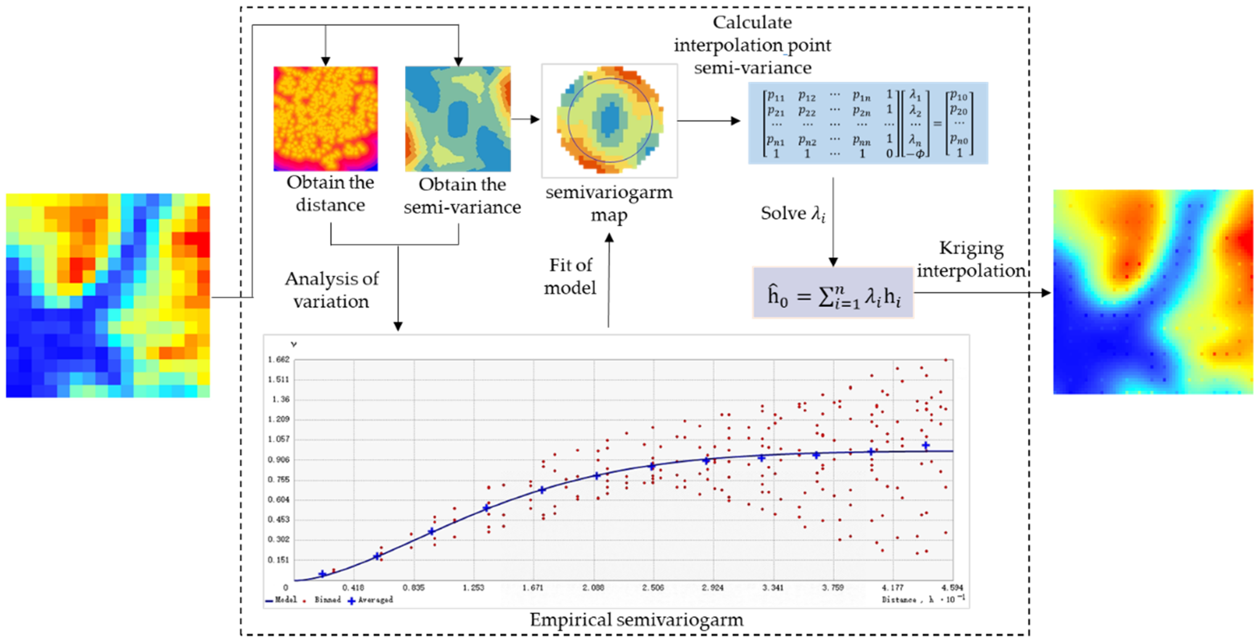
As a supplement method of DEM SR, the constraints provided by spatial autocorrelation can directly provide the DEM SR results with a certain degree of accuracy for the model. For example, the Kriging method [30] is used to find the spatial interpolation kernel that conforms to the target region by calculating the relationship between the spatial distance and the semi-variogram, and its interpolation results are highly accurate.

(2)

The results generated under the spatial autocorrelation rule are involved in the final results of the DEM SR, which is based on constraining the parameter flow direction of the learnable convolution kernel throughout the whole network, which indirectly supplements the global information for the model.

Although existing DEM SR methods have a good learning ability, they remain insufficient for the realistic restoration of terrain features. We argue that the problem arises from the lack of global terrain information, and hence, we propose a global-information-constrained deep learning network for DEM SR (GISR). Our model is designed for the purpose of the extraction and supplementation of global information. Specifically, there are two modules in the proposed GISR. First, a global information supplement module based on the Kriging method adds missing global information, whereas a local feature generation module is proposed for terrain feature extraction and recovery. In addition, a collaborative loss is adopted to supervise the training process and to optimize the parameter learning direction. The main contributions of our paper are summarized as follows:

• We propose a global-information-constrained deep learning network for DEM SR (GISR) that can optimize the DEM SR process toward generating global terrain features and achieving advanced results. Specifically, compared with the traditional bicubic Kriging interpolation method and existing neural network methods (TfaSR [31], SRResNet [32], and SRCNN [33]), the RMSE of our results is improved by 20% to 200%, and the MAE of our results is improved by 20% to 300%.
• We use the Kriging interpolation method, which accounts for spatial autocorrelation, to construct the global information supplement module. The module directly fuses the global information of the interpolation method and indirectly supplements the global information by affecting the loss to generate a DEM more similar to the real terrain distribution.

The rest of this paper is organized as follows: Section 2 is a review of the work related to the SR approach. In Section 3, we detail our proposed approach. In Section 4, the design of the experimental evaluation is described, and the results and analysis are presented. Section 5 is a discussion of the advantages and limitations of the proposed approach. In Section 6, we present our conclusions and discuss future work. The source code and data we have developed to implement our method are shared on Figshare (https://doi.org/10.6084/m9.figshare.21384093, accessed on 30 November 2022).

2. Related Work

2.1. Super-Resolution (SR) Based on Traditional Spatial Interpolation Methods

Spatial interpolation is a traditional SR operation that aims to predict the value at an unobserved location given some sampled data at observed locations [34]. Based on different hypothesis theories, classical spatial interpolation methods include the distance-weighted reciprocal method [35], natural nearest neighbor method [36,37], spline interpolation method [38,39], bicubic method [40,41], and Kriging method [10,30,42]. More specifically, the IDW (inverse distance weighted) interpolation method assumes that each sampling point has a certain local influence ability; the natural nearest neighbor method assumes that the sample points are unevenly distributed, which makes it an average weight algorithm that can be used for DEM SR [31]; spline interpolation [38] assumes that the surface attribute is gradual, and that the interpolation is realized by fitting a surface with minimum curvature that is valid on the terrain [43]. As a common DEM interpolation method [13], the bicubic interpolation method assumes that the change rate of each adjacent point value follows a specific distribution, and the corresponding parameters can be determined by known data; the Kriging method [30] assumes that the distance and direction between sample points reflect a spatial relationship that explains the spatial variation. Kriging includes many methods that can be divided into methods by characterizing the spatial structural features by estimating the semi-variogram cloud (simple Kriging method and ordinary Kriging) and by combining a regression of the dependent variable on auxiliary variables with the simple Kriging of the regression residuals (regression Kriging and general Kriging) [7]. Among the classical terrain interpolation algorithms mentioned above, the Kriging interpolation often performs better than others in situations of large-scale complex terrain interpolation because it can determine the interpolation kernel that is closer to the spatial distribution of the target region by finding an appropriate distance and semi-variogram. However, considering computational complexity and stability in practical applications, the bicubic interpolation method is commonly used for image super-resolution tasks.

2.2. DEM SR Based on Deep Learning Methods

The DEM SR method based on deep learning obtains the convolution kernel parameters closest to the spatial distribution of the target region by training massive homogeneous data, which enables it to complete the DEM SR task. This method’s creation cannot be separated from the development of deep learning technology in the field of computer vision. Specifically, the emergence of CNNs [20,21] helped scholars realize the feasibility of generating high-level semantic information from low-level features through multilevel feature transmission (in a feature extraction and feature recovery manner). However, due to the information loss of the pooling layer [44,45] and the mechanism of the full connection layer [46], the output of the CNN structure at this time is mainly a patch-wise network, which is more useful in scene classification [45,47,48], semantic segmentation [49,50], and object detection [51,52]. However, the introduction of FCNs (fully convolutional networks) [53] changed this situation. FCNs replaced pooling and full connection layers with convolutional layers, reducing the loss of high-level semantic information, and successfully promoting pixel-wise output, which made it possible to use FCNs for SR tasks. Inspired by the above network framework, scholars in the field of image super-resolution have proposed SRCNNs [33] and GANs, which are networks that surpass conventional interpolation methods. Considering the similar organizational structure of DEMs and images, scholars introduced SRCNNs [6], D-SRGANs [17], and CEDGANs [7] based on analogies and achieved better performances than interpolation-based SR methods. Limited by the degradation and vanishing gradients of the deep network, the above methods can only aggregate limited high-level semantic information through the shallow network, and the accuracy bottleneck soon appears. This problem was soon alleviated by ResNet [28] in the field of computer vision. Zhou et al. [16] applied this module and proposed an enhanced double-filter deep residual neural network (EDEM-SR) method that can capture more DEM features by introducing residual structures to deepen the network depth and enhance the ability to capture DEM features. Zhang et al. [12] also verified that the deep [23] network with a ResNet structure could achieve better DEM SR performance. Furthermore, Zhang et al. [36] considered the characteristics of DEM features and introduced a deformable convolution module, which was a breakthrough with regard to the limitation of the convolution kernel morphology and could enhance the ability to capture irregular DEM features; thus, the authors proposed that more DEM features could be retained. In addition, some novel DEM SR methods have also emerged. For example, Demiray et al. [54] created a DEM with an SR that was 16 times higher by improving MobileNetV3; Lin et al. [55] introduced the internally learned ZSSR (zero-shot super-resolution) method to solve the DEM SR task; Zhang et al. [56] proposed the recursive sub-pixel convolutional neural networks (RSPCNs) which have obvious improvements in both accuracy and robustness; and He et al. [57] introduced a Fourier transform as an encoder and acquired a good performance, which can enrich the existing DEM SR task encoder.

3. Methods

To further improve the DEM SR performance, we propose the global-information-constrained deep learning network for DEM super-resolution (GISR). Specifically (see Figure 2), in this method the LR DEM (low-resolution DEM, 16 × 16) is preprocessed. The size of the DEM is expanded to 64 × 64 using systematic sampling [7]. Additionally, the sampling data are changed into input DEM data (64 × 64) through ordinary Kriging interpolation. We used different variogram models (linear, power, gaussian, spherical, and exponential) and selected the best prediction results as samples. The preprocessed DEM is used as input for the local feature generation module, and the 64 × 64 DEM is the output at full size, which can be obtained through ResNet and PixelShuffle. Next, the 16 × 16 low-resolution DEM is used as input for the global information supplement module. Further, the DEMs generated by the global information supplement module and the local feature generation module are combined to obtain the final result. In addition, the collaborative loss is applied to optimize the training director of the model.

3.1. Global Information Supplement Module

The global information supplement module plays a direct (sampling the smooth DEM) and indirect (constraining the corresponding deep learning network parameters) role, and thus, it is important to find an interpolation kernel that is very close to the terrain law. Among the existing interpolation kernel methods, the Kriging interpolation kernel has the best performance. Kriging interpolation [10,30,42] is a classical method based on Tobler’s first law of geography [18,58] (geographical objects or attributes are interrelated in a spatial distribution, usually called spatial autocorrelation), which makes full use of the spatial correlation between the original data of regionalized variables and carries out an unbiased optimal estimation for the values of regionalized variables at noncamping points. To implement the Kriging interpolation method, we need to define the operations.

First, determine the terrain distribution mode in the region. According to the first law of geography, there is a relationship between known points. The ordinary Kriging method assumes that this relationship can be expressed as a function of distance and semi-variance between two pairs of known points, where distance represents spatial proximity, and semi-variance represents a spatial attribute. By drawing scatter plots of all distances $d_{ij}$ and semi-variances $p_{ij}$, the relationships of functions can be fitted, such as linear, quadratic, exponential, and logarithmic relationships. Define the distance formula between the known point i $\left(x_i,y_i\right)$ and the known point j $\left(x_j,y_j\right)$ as follows:

$$d_{ij}=d\left(\left(x_i,y_i\right),\left(x_j,y_j\right)\right)=\sqrt{{(x_i-x_j)}^2+{(y_i-y_j)}^2}$$

(1)

The semi-variance formula is as follows [38]:

$$p_{ij}=\frac{1}{2}E\left[{\left(h_i,h_j\right)}^2\right]={\sigma }^2-Cov\left(h_i,h_j\right)$$

(2)

where $h_i$ is the elevation value of point i $\left(x_i,y_i\right)$, $h_j$ is the elevation value of point j $\left(x_j,y_j\right),cov\left(h_i,h_j\right)$ is the covariance of point i $\left(x_i,y_i\right)$ and point j $\left(x_j,y_j\right)$, ${\sigma }^2$ is variance of point i $\left(x_i,y_i\right)$ and point j $\left(x_j,y_j\right)$.

The basic formula of Kriging interpolation is:

$${\widehat{h}}_0={{\displaystyle \sum }}_{i=1}^n{\lambda }_i{h}_i$$

(3)

where ${\widehat{h}}_0$ is the unbiased estimate of the point $\left(x_0,y_0\right)$; the ${\lambda }_i$ weight coefficient is the estimated value at the point that can be satisfied,${\widehat{h}}_0$; and the true value $h_0$ is the smallest set of optimal coefficients:

$$\underset{{\lambda }_i}{min}Var\left({\widehat{h}}_0-h_0\right)$$

(4)

Under the assumption of homogeneous spatial attributes and the premise of unbiased estimation, the cost function of obtaining the optimization objective is

$$J=Var\left({\widehat{h}}_0-h_0\right)=Var\left({{\displaystyle \sum }}_{i=1}^n{\lambda }_i{h}_i-h_0\right)$$

(5)

It is solved by using Lagrange multiplier method, and the solution method is to construct a new objective function:

$$J+2\varphi \left({\displaystyle \sum }_{i=1}^n{\lambda }_i-1\right)$$

(6)

where $\varphi$ is the Lagrange multiplier. Solving the parameter set $\varphi$ and ${\lambda }_i$ that minimize the cost function can satisfy the requirement that they minimize J under ${{\displaystyle \sum }}_{i=1}^n{\lambda }_i=1$ constraint:

$$\begin{array}{c}2p_{k0}-{{\displaystyle \sum }}_{j=1}^n\left(p_{ki}+p_{jk}\right){\lambda }_j+2\varphi =0;k=1,2,\cdots ,n\\ {{\displaystyle \sum }}_{i=1}^n{\lambda }_i=1\end{array}$$

(7)

After a series of derivations and calculations, the following weight matrix can be obtained:

$$\left[\begin{array}{ccccc}{p}_{11}& p_{12}& \cdots & p_{1n}& 1\\ p_{21}& p_{22}& \cdots & p_{2n}& 1\\ \cdots & \cdots & \cdots & \cdots & \cdots \\ p_{n1}& p_{n2}& \cdots & p_{nn}& 1\\ 1& 1& \cdots & 1& 0\end{array}\right]\left[\begin{array}{c}{\lambda }_1\\ {\lambda }_2\\ \cdots \\ {\lambda }_n\\ -\Phi \end{array}\right]=\left[\begin{array}{c}{p}_{10}\\ p_{20}\\ \cdots \\ p_{n0}\\ 1\end{array}\right]$$

(8)

To solve for the elevation value of unknown points, first, use the fitting function of distance and semi-variance and calculate $p_{i0}$ according to the distance from the interpolation point to all known points, then inverse the above matrix to obtain all the weight coefficients, and finally, bring back the basic formula of Kriging interpolation,${\widehat{ h}}_0={{\displaystyle \sum }}_{i=1}^n{\lambda }_i{h}_i$. Thus, the elevation value of the interpolation point is obtained. The approximate flow of the Kriging interpolation method is shown in Figure 3.

3.2. Local Feature Generation Module

The local feature generation module was designed to retain the terrain details and to reproduce a more realistic geographical distribution pattern. The local feature generation module inputs the 64 × 64 low-resolution DEM generated by the global information supplement module. First, the convolution layer (kernel size = 9, padding = 4, and stride = 1) is used based on the relatively large receptive field (9 × 9). The terrain features are extracted and then activated using the PReLU (parametric rectified linear unit) [53]. Then, the extracted features flow into the residual module. Next, the features pass through a roll-up layer (kernel size = 3, padding = 1, and stride = 1) and a BN (batch normalization layer) [59] again. The features and residual blocks obtained in this step are extracted for stacking, and the stacked features flow into the upper sampling module as input. The upper sampling module consists of four layers, namely, the convolution layer (kernel size = 3, padding = 1, and stride = 1), batch normalization layer (BN), PixelShuffle [24] layer (factor = 2), and PReLU activation layer. The feature size passes through the convolution layer (kernel size = 9, padding = 4, and stride = 2) and the Tanh [60] layer.

Among them, the PReLU [53] layer is selected as the active layer because it can adaptively learn and correct the parameters of linear units and improve accuracy with negligible additional computing costs. Additionally, the PReLU can avoid zero gradients, unlike the LReLU [61]. The experiment shows that, compared with the ReLU [62], the precision of the LReLU is almost not improved. At the same time, PReLU parameters can be learned adaptively, which improves the learnability of the network. The PReLU only adds a small number of parameters, which means that the calculation amount of the network and the risk of overfitting only increase a little, particularly when different channels can use the same parameters. In addition, to further optimize the extracted features, we added a full convolution network to the network to preserve the terrain details extracted from the receptive field and constrain the training director of the model. Next, we will introduce the relevant concepts of the residual feature extraction module and PixelShuffle in detail.

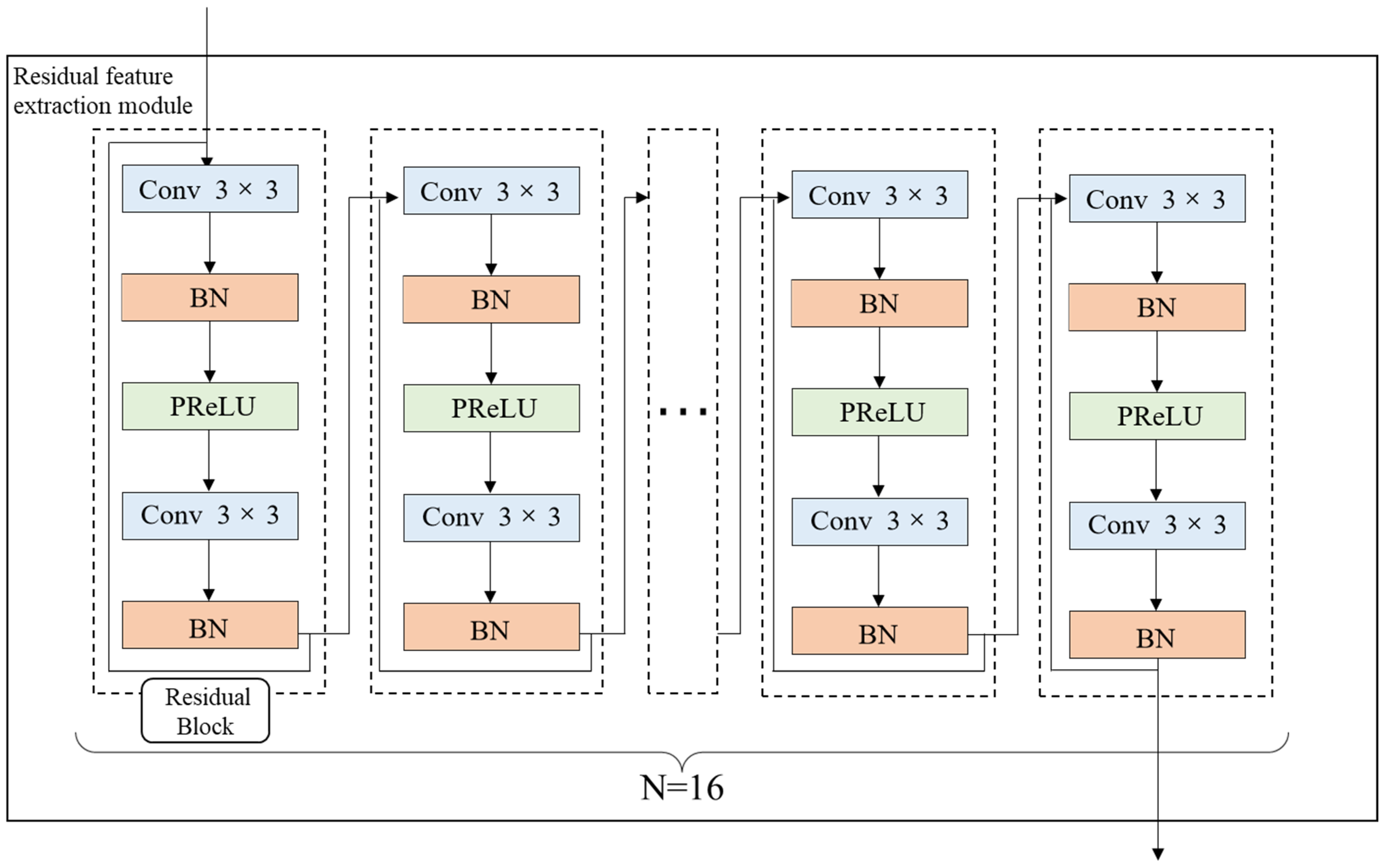
3.2.1. The Concept of the Residual Feature Extraction Module

With the deepening of the deep learning network, the problems of vanishing gradients, exploding gradients, and degradation are gradually emerging. The ingenious design of the ResNet network effectively alleviates these problems and creates the possibility of building a deeper and more complex network [22,23]. ResNet introduces a jump connection structure, which allows some layers of the neural network to skip the connection between neurons on the next layer and the current layer, weakening the strong connection between each layer. Specifically, it saves the parameter characteristics of the current layer before training and transfers these parameters and the data after training the last layer. In this way, some of the features of the previous layer are preserved, and convolution training can also be performed, effectively alleviating the problem of deeper network degradation. The gradient correlation is continuously attenuated with the increase in layers. The jumping of ResNet can effectively reduce the attenuation of this correlation, thus alleviating the problem of vanishing and exploding gradients [63]. In addition, batch normalization controls exploding gradients by standardizing data distribution to prevent vanishing gradients.

The residual feature extraction module is a sixteen-residual-block (n = 16) network module built according to ResNet. Each residual block contains five layers, including two convolution layers (kernel size = 3, padding = 4, and stride = 1), two batch normalization layers (BN), and a linear correction unit (PReLU) activation layer with parameters. Specifically, the convolution layer is used to extract terrain features, and the BN layer is used to reduce the impact of extreme altitude (for example, very large and very small altitude values). It also solves the problem where the deep neural network is more difficult to train and converges more slowly as the network deepens. The activation layer is used to improve the stability and nonlinearity of network performance. Therefore, the proposed residual model can extract useful deep terrain features. The ResNet layer structure is shown in Figure 4.

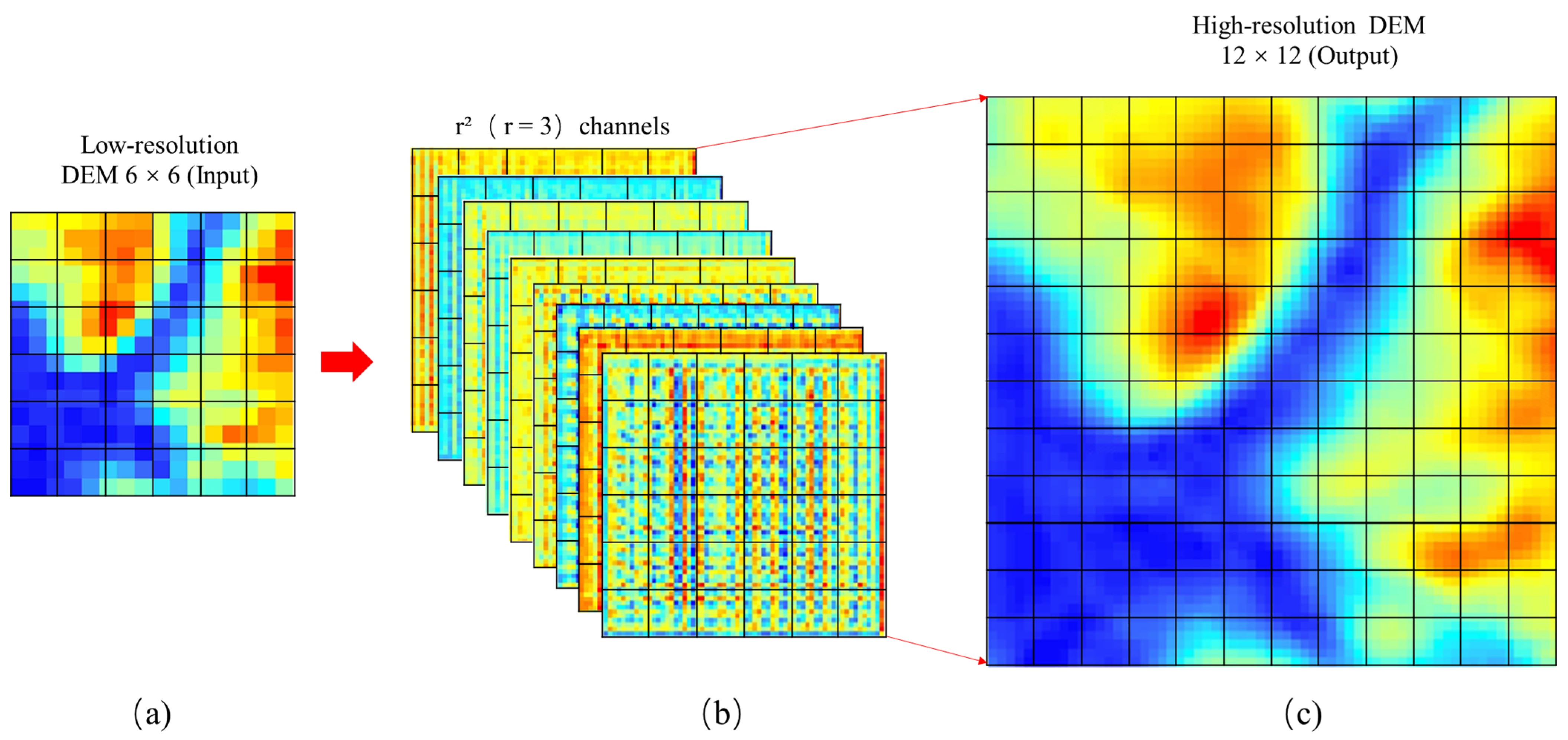
3.2.2. The Concept of PixelShuffle

PixelShuffle [24] (sub-pixel convolutional neural network) is used to obtain high-resolution feature maps from low-resolution feature maps through sub-pixel convolution and multichannel recombination. This paper uses it as a feature up sampling method.

Assume the feature map $F_L$ of a low-resolution DEM has a size of h × w × c. The height and width of the feature map of the reconstructed high-resolution DEM are expanded r times, and the size is h * r × w * r × c. PixelShuffle convolves $F_L$ with a convolution kernel of depth c * r² to obtain a feature map of h × w × c * r². Additionally, it is then reorganized into h * r × w * r × c by PixelShuffle (PS), which is defined as follows:

$$\mathrm{PS}{\left(T\right)}_{x,y,c}=T_{\left[x/r\right], \left[y/r\right],C\ast r\ast mod\left(y,r\right)+C\ast mod\left(x,r\right)+c}$$

(9)

where T is the feature map of the input $r^2$ channels, each original low-resolution pixel is divided into $r^2$ smaller grids, and these grids are filled with the values of the corresponding positions of $r^2$ feature maps according to a certain rule (C and mod comprise the certain rule). The reorganization process is completed by filling the lattice and dividing it by each low-resolution pixel according to the same rules. The process of sampling DEM with PixelShuffle is shown in Figure 5.

3.3. Collaborative Loss

Image SR focuses on the visual perception of the reconstructed image, whereas the DEM pays more attention to the reproduction degree of terrain features and elevation accuracy [32]. Therefore, considering the extraction effect of terrain features and geographical rules, we designed a collaborative loss model. Our loss function can be divided into two parts: the first is the elevation loss, which is used to constrain the global elevation accuracy, and the second is the feature loss, which improves the terrain accuracy and retains the terrain features while accelerating the convergence. We chose L1 loss and RMSE loss to comprise the loss function, and the formulas are as follows:

$$L1\left(y_i,\widehat{y_i}\right)=\frac{1}{N}{{\displaystyle \sum }}_{i=1}^N\left|y_i-\widehat{y_i}\right|$$

(10)

$$RMSE \left(y_i,\widehat{y_i}\right)=\sqrt{\frac{1}{N}{{\displaystyle \sum }}_{i=1}^N{\left(y_i-\widehat{y_i}\right)}^2}$$

(11)

where $y_i$ represents the true elevation value, $\widehat{y_i}$ represents the predicted elevation value, and $N$ represents the number of pixels counted.

3.3.1. Elevation Loss

In work that applies DEM SR, elevation accuracy is very important, which is different from paying attention to the visual effects of general natural images. Therefore, elevation loss is added to improve the accuracy of the global terrain. In practical works, people often use the RMSE to measure DEM accuracy; thus, the RMSE is used here to represent elevation loss. The specific formula is as follows:

$$L_E=RMSE\left(h_i,\widehat{h_i}\right)$$

(12)

where $h_i$ is the original high-resolution DEM, and $\widehat{h_i}$ is a high-resolution DEM generated by the residual module.

3.3.2. Feature Loss

The loss function is an algorithm used to measure the feature gap between real data and generated false data, which constrains the direction of model training. The relevant formulas are as follows:

$$L_{F_v}=L1\left(v_i,\widehat{v_i}\right)$$

(13)

$$L_{F_c}=RMSE\left(I,C\right)$$

(14)

where $v_i$ is the terrain feature extracted from the original high-resolution DEM through the VGG [64] module, $\widehat{v_i}$ is the terrain feature extracted from the high-resolution DEM generated by the residual module through the VGG module, $I$ is the matrix with all values of one, and $C$ is the feature extracted from the high-resolution DEM generated by the residual module through the full convolution module [32].

The loss of topographic features is composed of two parts, namely, $L_{F_v}\mathrm{and}{L}_{F_c}$:

$$L_F=L_{F_v}+\beta L_{F_c}$$

(15)

The loss function directly determines the direction of network optimization and affects the quality of final DEM generation. Therefore, multiple loss function collaborative constraints are designed. The collaborative loss is a combination of elevation accuracy loss and terrain feature loss, as shown below:

$$L_C=\alpha L_E+L_F$$

(16)

Among them, $\alpha$ and $\beta$ are the weight coefficients.

4. Experiments

4.1. Experimental Setup

This section describes the experimental setup, including datasets, parameters, selected comparison methods, and terrain indicators. First, we selected DEMs with complex terrain distribution (seen in Figure 6) to test the generalization of the proposed method. The resolution of the DEMs is 30 m, and the study area size is 7201 × 7201. It can be seen from the figure that the terrain elevation values range from 304 m to 2335 m, which is much larger than the range from 0 to 255 in the image field. The study area has a wide range of slopes, with the highest slope approaching 80 degrees and being mostly concentrated at 0–40 degrees. The area includes complex terrain features, such as ridges, valleys, rivers, cliffs, etc.

The terrain will change over time due to external effects; thus, it is a challenge to simultaneously obtain DEMs with different resolutions in the same area. Considering the experimental setup’s rationality and the experimental data’s availability, we need to conduct down sampling processing on the high-resolution DEM to obtain the corresponding low-resolution DEM. The down sampling factor was designed at 4, which is a commonly used target scale. Since the experimental setting is a 1:1 super-resolution, we need to restore the downsampled DEM to its original size. We used the Kriging method to complete the size restoration. The large DEM was cut into non-overlapping 64 × 64 single-channel small DEMs randomly, and 12,544 DEM fragments were obtained. To avoid overfitting the model, the DEM was uniformly extracted from each region using systematic sampling. The volume ratio of the training set and test set was 8:2, which means that 10,035 DEMs were sampled as training data and 2509 DEMs as test data. To enhance the persuasiveness of the experiment, we selected four different types of areas in the test set for the test demonstration. Specifically, Figure 7contains raw DEM data, elevation statistics, slope statistics, and horizontal and vertical drop distributions. Using the DEM parameter information in Figure 7, we can intuitively find the difference between them: The overall elevation (about 600–1000 m) and elevation range (about 500 m) of R1 and R2 are roughly similar, but the terrain distribution of R1 is slightly flatter than R2 (the R1 slope is concentrated at 0–10 degrees, and R2 at 10–30). The overall elevation of R3 is the smallest (about 100–700 m), the elevation range is close to R1R2 (513 m), and the topographic relief is large. The overall elevation of R4 is close to that of R1R2 (about 600–1000 m), but the elevation difference is the smallest (171 m), and the slope is also concentrated at 0–10 degrees, which is a relatively smooth area.

To shorten the test time, we chose the 64 × 64 small-sized DEM, but this does not mean that our model can only be effective for this size. We used the PyTorch platform to train and test the network and the Adam optimizer (with a batch size of 16) to replace the classical random gradient descent method to update the network weight more effectively [65]. The learning rate for backpropagation was set as 0.0002, and the network was trained with 100 epochs. The weights of loss were set as α = 1 and β = 0.01 to balance out their value scales.

Then, to evaluate our network’s effectiveness, we compared it with several common DEM super-resolution methods, including classical interpolation methods and deep learning network methods. The commonly used classical interpolation methods include nearest neighbor interpolation, bilinear interpolation, bicubic interpolation, cubic B-spline interpolation, etc. The research of Han et al. showed that bicubic interpolation produces the best image effect, and it is usually used as a baseline to evaluate the effect of the SR method; therefore, we chose the bicubic [8], Kriging [42], SRResNet [32], TfaSR [31], and SRCNN [6] methods to test the deep learning network.

This paper evaluates the results of DEM super-resolution based on three indicators: elevation [56], slope [31,66], and SSIM (structure similarity index measure) [67]. The calculation formulas for the slope (Formulas (17)–(19)) and SSIM (Formulas (20)–(22)) are as follows:

$$dx=\frac{\left[\left(e_{i-1,j+1}+2e_{i,j+1}+e_{i+1,j+1}\right)-\left(e_{i-1,j-1}+2e_{i,j-1}+e_{i+1,j-1}\right)\right]}{8\times Cellisize}$$

(17)

$$dy=\frac{\left[\left(e_{i+1,j-1}+2e_{i+1,j}+e_{i+1,j+1}\right)-\left(e_{i-1,j-1}+2e_{i-1,j}+e_{i-1,j+1}\right)\right]}{8\times Cellisize}$$

(18)

$$slop{e}_{ij}=arctan\sqrt{d{x}^2+d{y}^2}$$

(19)

$$SSIM\left(x,y\right)=\frac{2{\mu }_x{\mu }_y+C_1}{{\mu }_x^2+{\mu }_y^2+C_1}·\frac{2{\sigma }_{xy}+C_2}{{\sigma }_x^2+{\sigma }_y^2+C_2}$$

(20)

$$C_1={\left(k_{1}L\right)}^2 k_1=0.01$$

(21)

$$C_2={\left(k_{2}L\right)}^2 k_2=0.03$$

(22)

In Formulas (17)–(19) [31,66], $e_{i,j}$ denotes the elevation of the cell $\left(x_i,y_j\right)$, $Cellisize$ denotes the resolution of the DEM, and $slop{e}_{ij}$ denotes the slope of the DEM. In Formula (20) [67], ${\mu }_x$ and ${\mu }_y$ are the mean of x and y, respectively; ${\sigma }_x$ and ${\sigma }_y$ are the standard deviation of x and y, respectively; ${\sigma }_{xy}$ is the covariance of x and y; and $C_1$ and $C_2$ are fixed parameters used to maintain the stability of Formulas (21) and (22) [67], where L is the maximum value of the pixel (L ≈ 255, due to normalization).

The specific evaluation methods include the mean absolute error (MAE) and the root mean square error (RMSE), and the formulas are as follows [13,68]:

$$MAE=\frac{1}{N}{{\displaystyle \sum }}_{i=1}^N\left|h_i-\widehat{h_i}\right|$$

(23)

$$RMSE=\sqrt{\frac{1}{N}{{\displaystyle \sum }}_{i=1}^N{\left(h_i-\widehat{h_i}\right)}^2}$$

(24)

where N denotes the number of pixels in the test samples, $h_i$ denotes the values in the original high-resolution DEM, and $\widehat{h_i}$ denotes the values in the reconstructed high-resolution DEM.

4.2. Training

This section details the training process. The training details shown in Figure 8 represent the variation in the average global elevation accuracy (RMSE-elevation). The abscissa is the epoch, and the ordinate is the loss value (Km). By observing the curve, we found that:

①

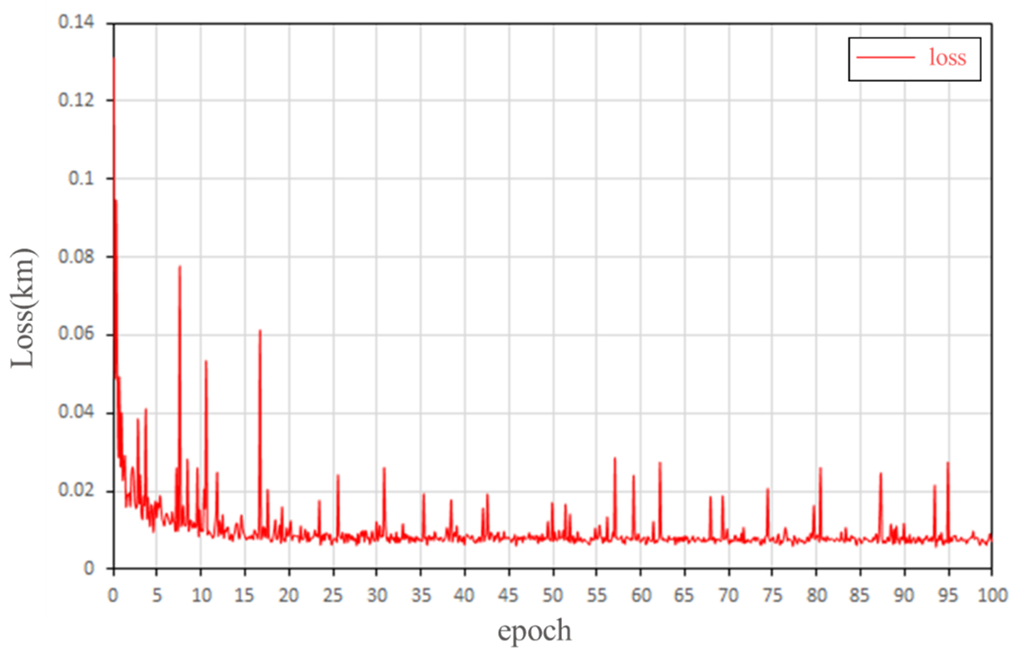
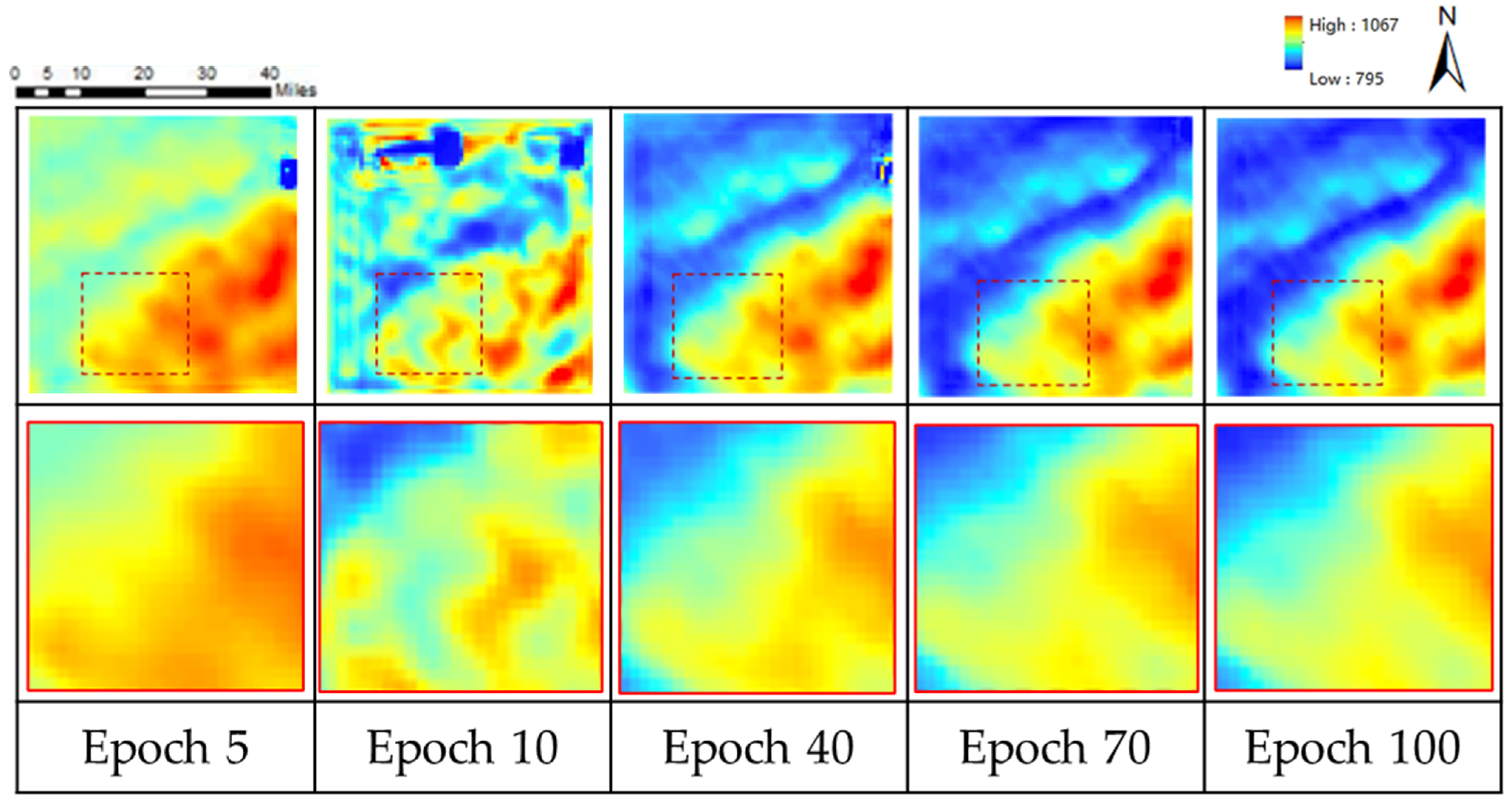
Figure 8 shows a downward trend, which decreases rapidly in the early stage and gradually flattens in the late stage. This phenomenon shows that our model can effectively capture the depth of the spatial terrain characteristics of the samples.

②

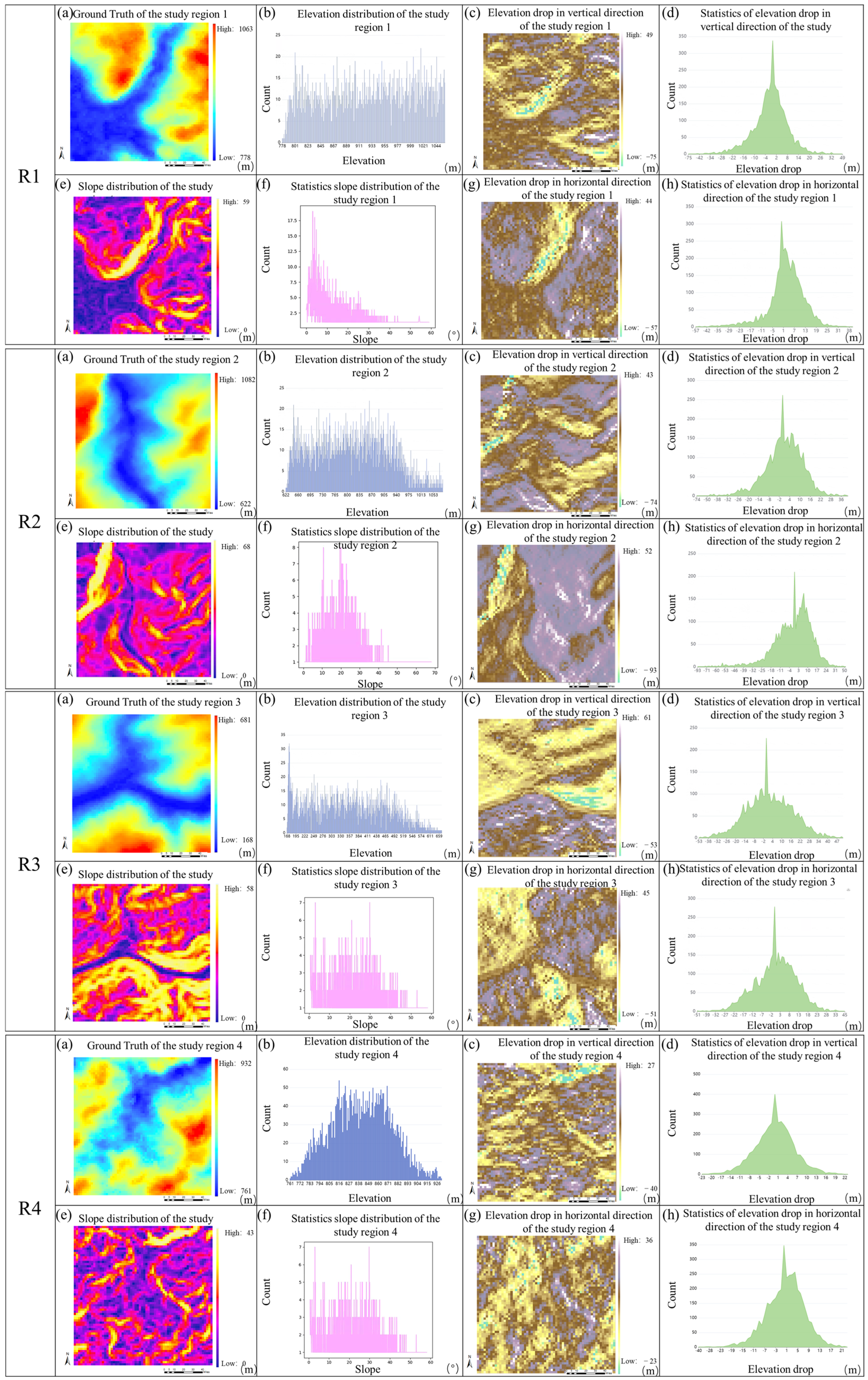
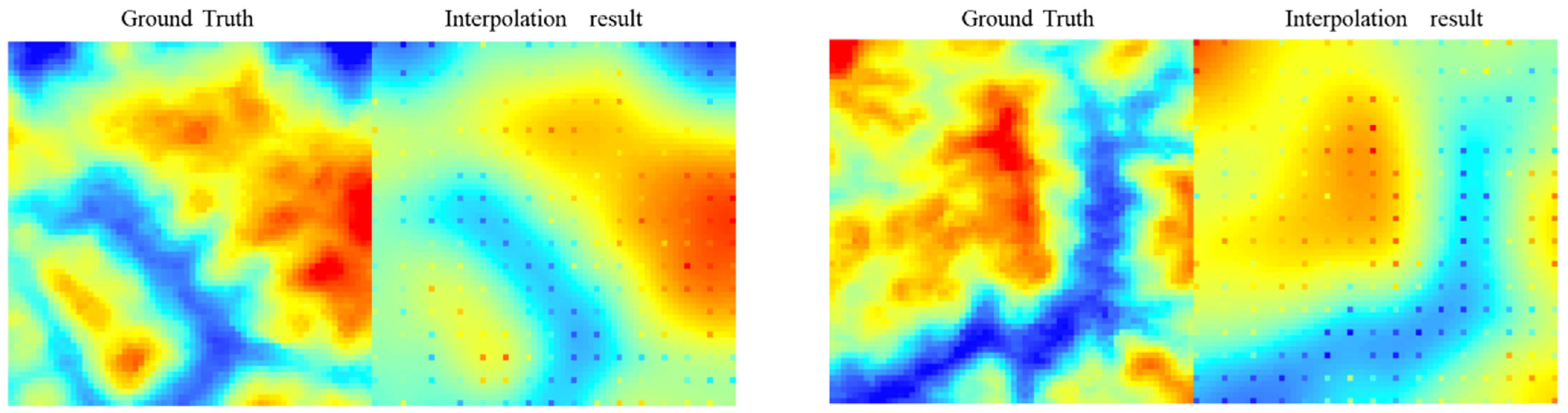
During the whole training process, the loss fluctuates up and down. At the initial stage of training, the initial waveform fluctuates greatly. When the training epoch increases, the performance of the DEM generation tends to be stable, and the fluctuation amplitude becomes smaller. There are two reasons for loss fluctuation: (1) In the training process, the randomly selected samples come from different regions, and their elevation drop and terrain complexity are different, leading to the instability of loss. (2) The preprocessing effect of some regions with too complex terrain is not good (Figure 9), resulting in a large loss value of the generated results, which makes the loss fluctuate. It is proved by experiments that the results of training after removing the problematic samples from the preprocessing are almost the same as those of training with all samples.

Next, Figure 10 shows the effect of the model terrain generation over different training periods. It is observed that that the terrain recovery degree gradually improves during the whole training process. After 5 epochs of training, the overall effect of the DEM was restored, and as the training continues, the generated DEM had more fine details as it reached 10 epochs. After 40 epochs, the model had reproduced most of the topographic features and geographical spatial patterns. By the 70th epoch, the visual effect of the generated DEM was no different from that of the real high-resolution DEM, and the super-resolution task was completed. After that, the effect of training was improved with little effect.

5. Results and Discussions

5.1. Results

In this section, we will use untrained samples as test data to test the effect of our proposed network. For a more objective explanation, we use classical interpolation methods (bicubic interpolation and Kriging interpolation) and deep learning networks (SRResNet and TfaSR) to conduct a comparative experimental analysis with our proposed model. The deep learning networks and our model are trained for 100 epochs to ensure fairness. The overall accuracy, visual effect, and terrain feature retention will be comprehensively compared and explained.

5.1.1. Overall Accuracy

In this section, we evaluate the overall accuracy. We compare the bicubic interpolation, Kriging interpolation, SRResNet, TfaSR, and SRCNN, with our methods in two different test areas to prove the effectiveness of our proposed model. A series of indicators reflect the elevation and slope, and the MAE and RMSE are used to measure the accuracy, whereas the SSIM is used to measure the structural similarity.

It can be seen in

Table 1. The accuracy indicators of different methods.

Region	Method	MAE		RMSE		SSIM
		Elevation	Slope	Elevation	Slope
R1	Bicubic [40]	14.958	6.405	21.120	8.547	0.789
	Kriging [42]	9.870	6.310	13.143	8.163	0.851
	SRResNet [32]	7.493	5.124	10.165	6.684	0.890
	SRCNN [6]	7.560	5.235	9.926	6.971	0.859
	TfaSR [31]	10.730	6.565	13.908	8.665	0.793
	GISR	6.365	4.503	8.236	5.824	0.919
R2	Bicubic	25.064	8.289	35.994	11.374	0.835
	Kriging	11.546	6.562	16.193	8.831	0.913
	SRResNet	8.553	5.235	11.630	6.665	0.927
	SRCNN	9.221	5.644	12.728	7.225	0.945
	TfaSR	12.578	6.773	16.598	8.587	0.905
	GISR	6.232	4.424	8.364	5.581	0.971
R3	Bicubic	22.462	7.148	27.365	9.165	0.847
	Kriging	13.217	7.884	17.526	8.981	0.872
	SRResNet	16.568	6.825	25.054	8.919	0.901
	SRCNN	11.343	6.181	14.379	7.839	0.935
	TfaSR	14.122	7.041	17.449	8.763	0.908
	GISR	7.785	4.628	9.865	5.910	0.956
R4	Bicubic	11.002	5.460	14.577	7.118	0.705
	Kriging	9.276	6.659	12.153	7.885	0.676
	SRResNet	7.146	5.029	9.606	6.439	0.791
	SRCNN	8.151	6.048	10.438	7.684	0.770
	TfaSR	10.840	6.675	14.017	8.551	0.548
	GISR	4.871	3.854	6.316	4.951	0.885

that: (1) In the test regions R1, R2, R3, and R4, the performance of the GISR method proposed in this paper is superior to the compared methods in elevation, slope, and SSIM. (2) In the traditional interpolation method, Kriging’s evaluation indices in this section are better than the bicubic ones. It is easy to understand because the Kriging method considers the global spatial autocorrelation better, whereas the bicubic method only establishes relationships with a few points around the mapping point (see Section 3 for details). Although the net result of SRCNN is simple, it is superior to TfaSR, SRResNet, and other deep learning networks with complex structures in some test regions.

In conclusion, the results show the effectiveness of the proposed GISR method, as it has a good performance in regard to the DEM SR tasks in complex regions.

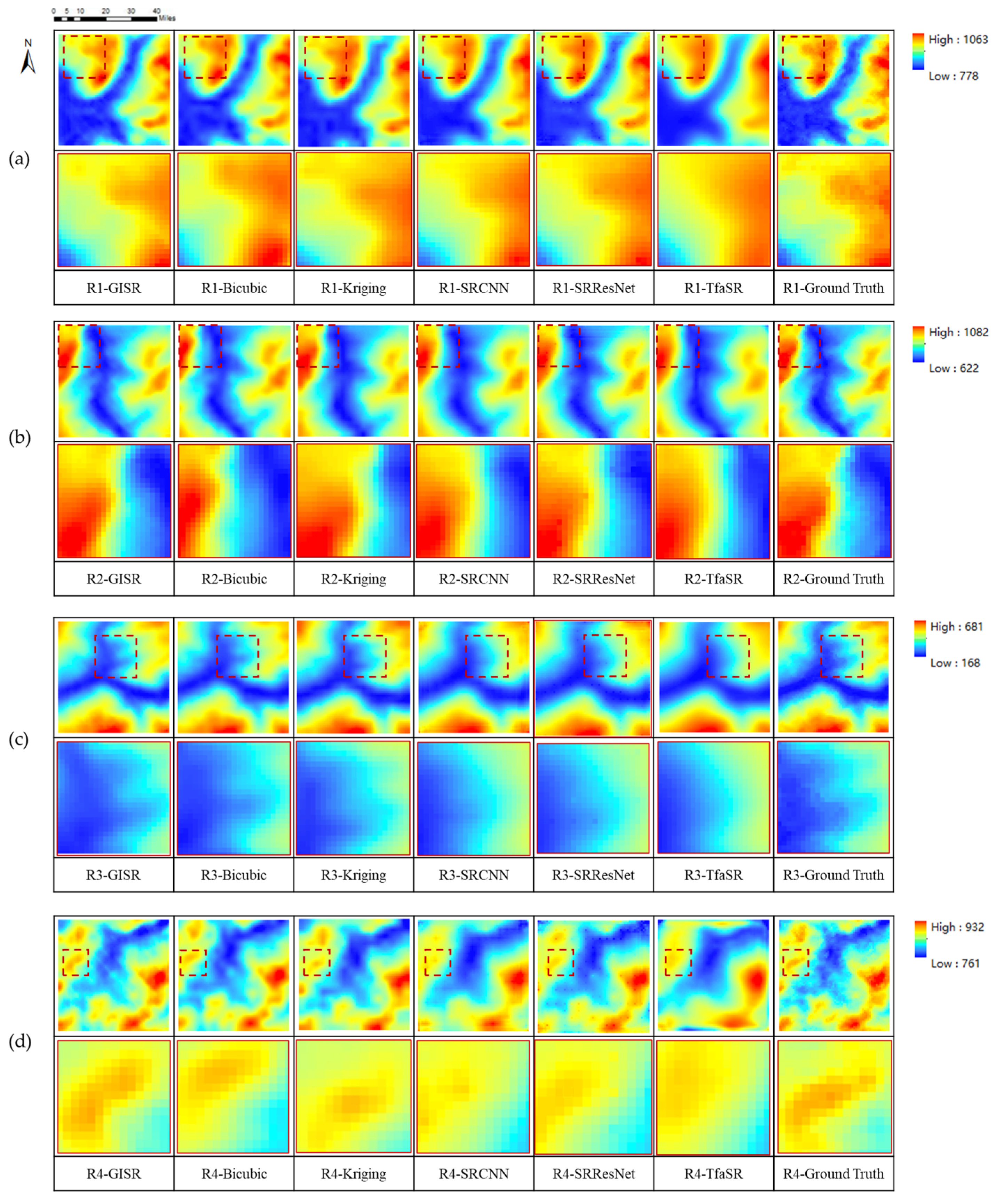
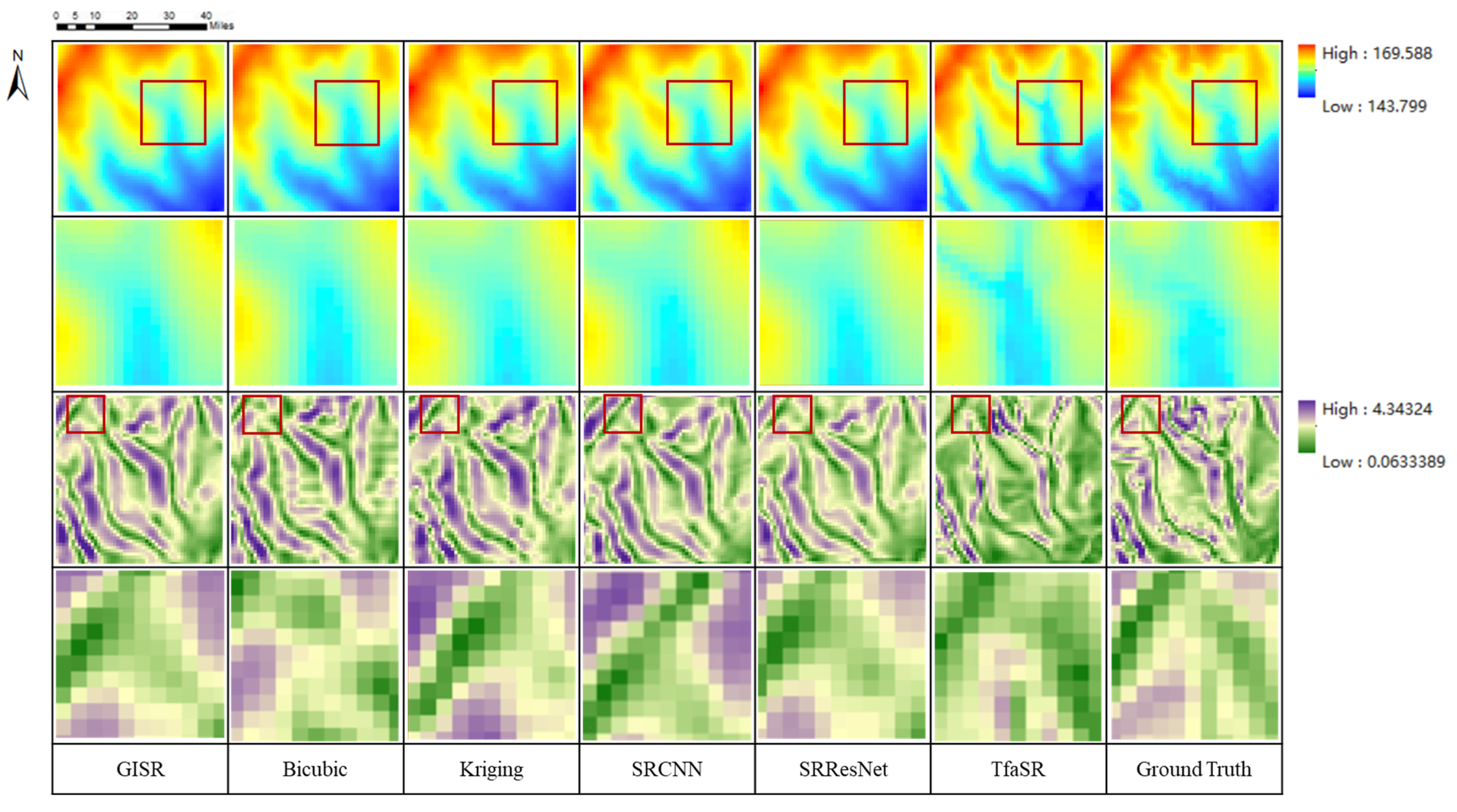
5.1.2. Visual Assessment

From the perspective of quantitative evaluation, GISR is superior to other methods where visual evaluation is required because, in many cases, images with better quantitative indicators have poor visual perception. The high numerical accuracy of a DEM does not mean better quality. A DEM that is too smooth often performs well in numerical accuracy, but the cost of smoothing is the loss of terrain details. Therefore, to evaluate the quality of a DEM, it is necessary to evaluate the degree of detail retention of topographic features.

In Figure 11, it can be seen that the TfaSR results show excessive smoothness that is even worse than that of the traditional bicubic interpolation method, which performs poorly with regard to precision numerical values. The Kriging method, which reflects the global terrain features, presents the phenomena of overall smoothness and the loss of terrain details. However, it is worth noting that there is an abrupt change in elevation between the known sample data points and the surrounding interpolation estimation points, resulting in a discontinuous visual terrain. Similar to the numerical accuracy results, SRCNN and SRResNet perform satisfactorily in detail retention. The experimental results show that our GISR method retains more terrain details in the test regions than other methods and restores the terrain distribution law of the real DEM.

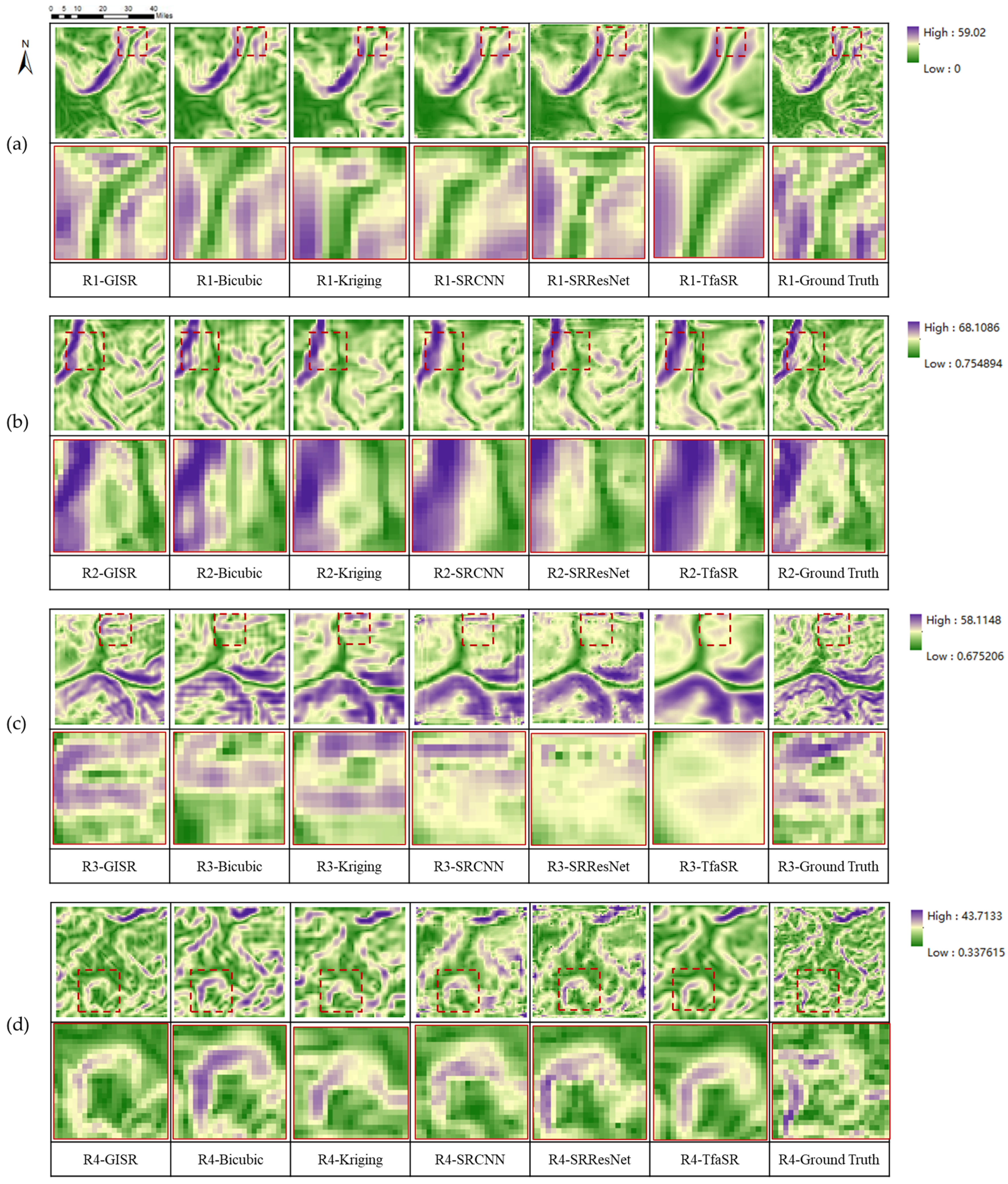
5.1.3. Terrain Parameter Maintenance

The slope is an important indicator when measuring the terrain features. We use the slope to further evaluate the feature retention of the generated DEM. The comparison with the slope of the real terrain shows the ability of different methods to maintain the terrain features.

In Figure 12, the restoration of terrain features by different methods is shown. The window frame phenomenon appears on the edge of SRCNN and SRResNet. The over-smoothing of terrain features with TfaSR is particularly evident in the slope. The abrupt change between the Kriging data point and the interpolation point shows that the data point is similar to the noise point in the slope. The experimental results show that in the test area, our method retains more details of the terrain features (slope) than other methods and is closer to the terrain distribution of the real DEM.

5.2. Discussion

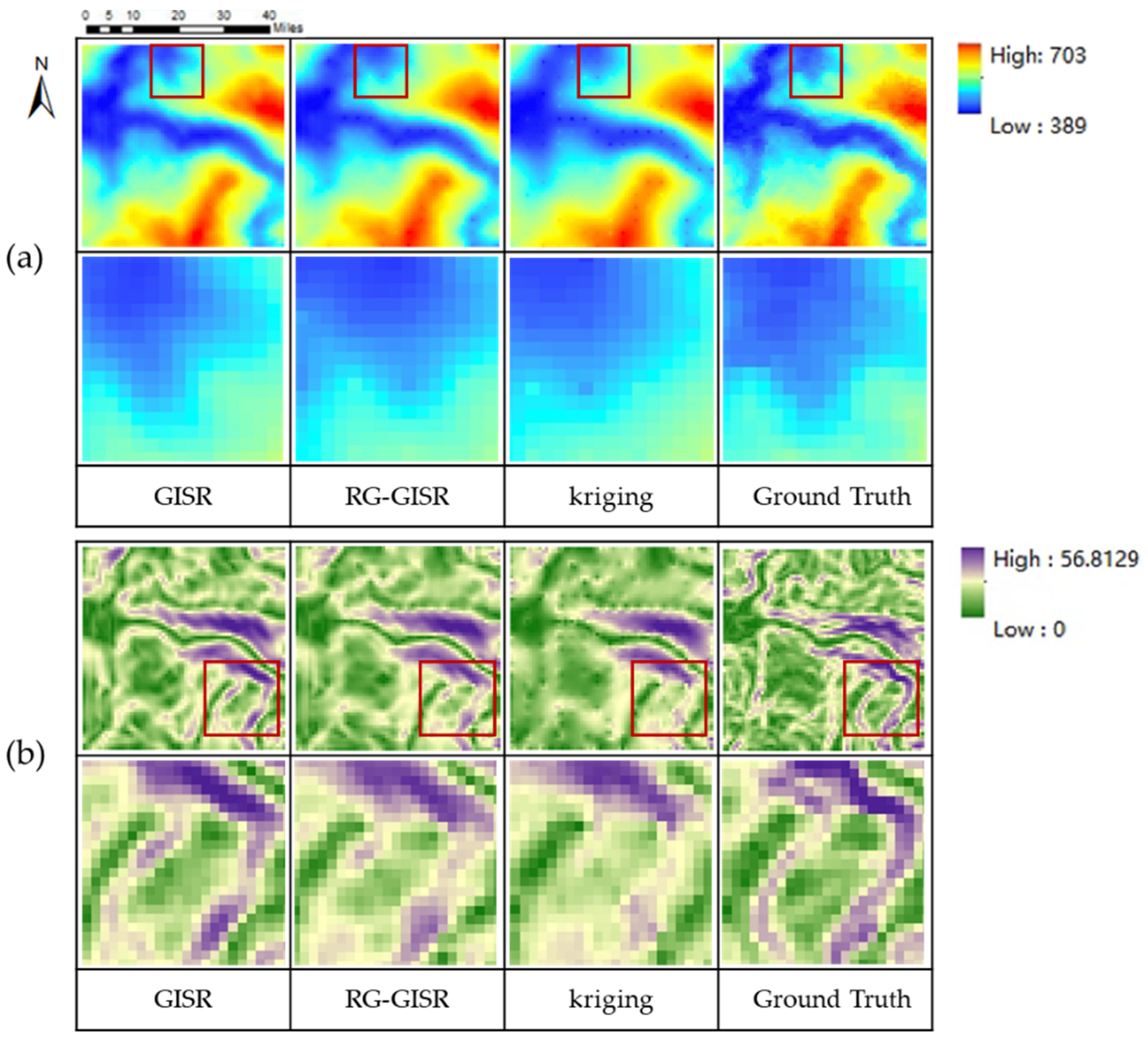
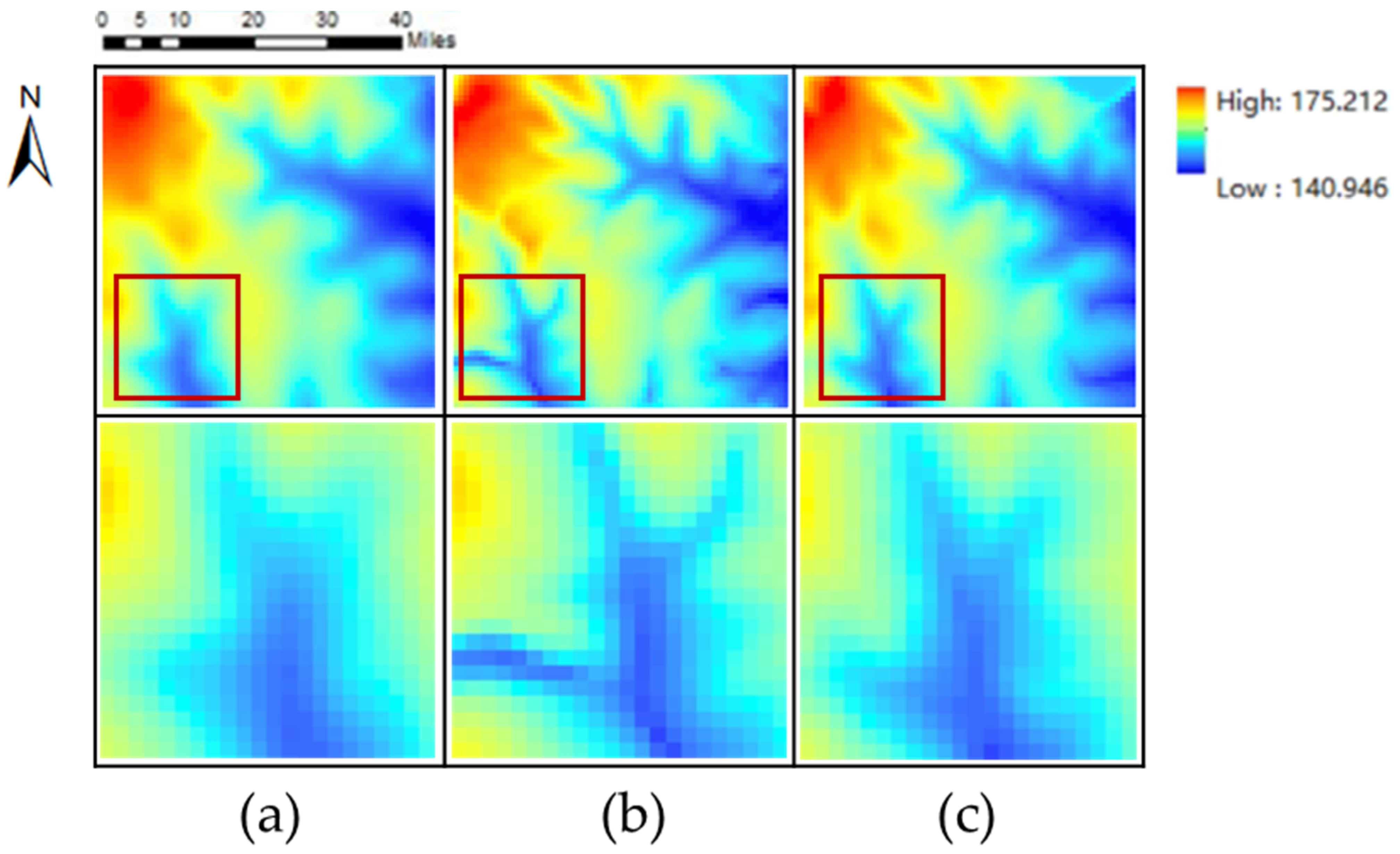
5.2.1. The Impact of the Global Information Supplement Module

Since the nature of terrain evolution is affected by long-term geological processes such as erosion and landslides, it has spatial autocorrelation. The Kriging interpolation algorithm takes spatial autocorrelation into account. We used this feature to design a global information supplement module to supplement certain transmission loss information and global information while taking spatial autocorrelation into account. In this section, we discuss the effectiveness of the global information supplement module.

It can be seen from

Table 2. The accuracy indicators of ablation experiments to remove different modules (GISR is a method in this paper, RG-GISR means removing the global information supplement module, Kriging as control method).

		GISR	RG-GISR	Kriging
MAE	Elevation	6.250	8.432	7.521
	Slope	4.845	5.010	5.873
RMSE	Elevation	8.178	10.387	10.121
	Slope	6.148	6.411	7.550

that the elevation accuracy of our GISR method (including the global information supplement module) is higher than that of the experimental group without this module and is also higher than that of the Kriging interpolation method. This shows that the overall network architecture we designed is reasonable, and the addition of the global information supplement module improved the elevation accuracy of the DEM. In addition, the analysis of the Kriging interpolation elevation accuracy shows that the results are not as good as our GISR method’s results. This may be due to the fact that the Kriging method takes spatial autocorrelation into account to give the DEM global features, but it lacks detailed terrain features and cannot restore the terrain undulation of the real DEM. The slope and elevation accuracy follow the same rule, which will not be repeated here. When the global information supplement module is removed, the slope direction accuracy is the highest. The RMSE is more sensitive to extreme values, and the MAE tends to describe the average state. The emphasis of the two is different, and therefore, the problems reflected are also different.

It can be seen from Figure 13 that our GISR method (including the global information supplement module) is more similar to the real terrain in terms of DEM and slope. The experimental group without this module will have incorrect feature information, and some features will not be recovered. As with the control group, the Kriging method’s overall terrain distribution still shows excessive smoothness and lacks details. To summarize, the global information supplement module effectively supplements the global information lost in the transmission process and also shows the rationality of our GISR design method.

In addition, in order to further explore the role of the global information supplement module in modeling long-distance geographic features (i.e., drainage lines), we further compared the GISR method and the GISR method (RG-GISR) that removes the global information supplement module in modeling drainage lines. The specific results are shown in Figure 14. By analyzing Figure 13, we can find that after removing the global information, RG-GISR overemphasizes local features (generating additional significant topographic features). On the contrary, GISR can constrain the generated results by modeling the drainage line through the global information module so that the generated geographic features are closer to the ground truth in the contour. In a word, more accurate modeling of long-distance geographic features is an important role of the global information module.

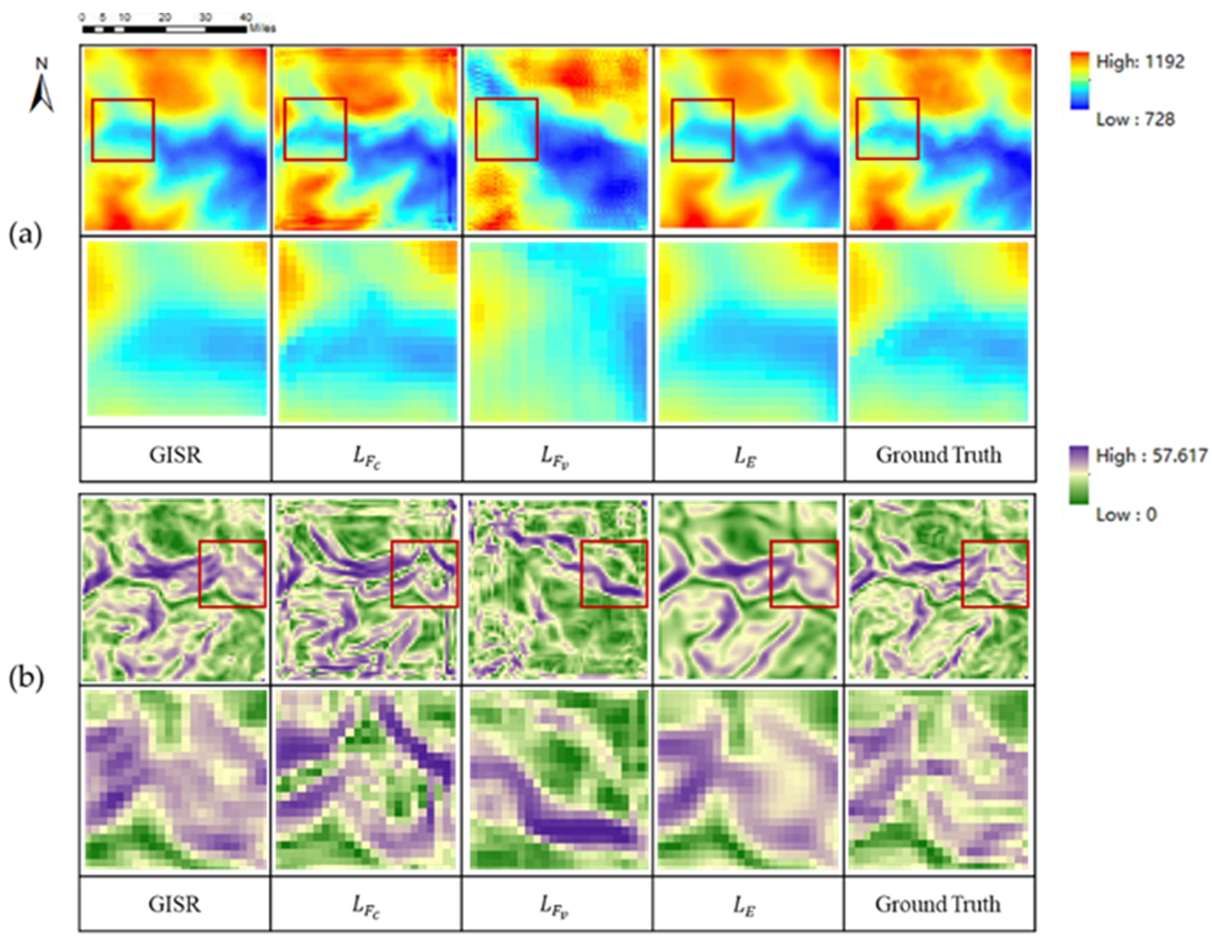
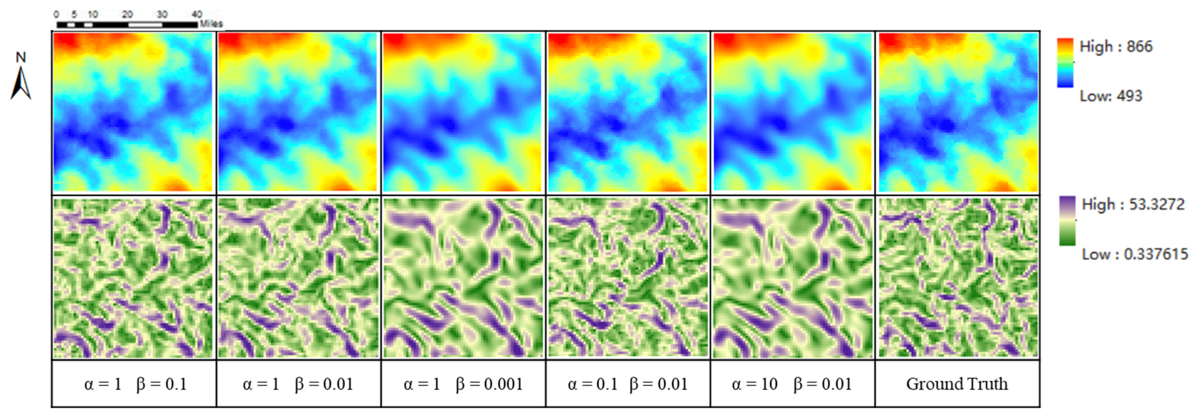
5.2.2. Effectiveness of the Collaborative Loss

The loss function is an algorithm used to measure the difference between the real data and the generated false data, which constrains the direction of model training. Therefore, we will discuss the role of the collaborative loss model. The collaborative loss in this paper is composed of elevation loss, $L_E,$ and feature loss, $L_{F_v} and L_{F_c}$. The effects of only $L_E$, $L_{F_c}$, $L_{F_v}$, and the original model were tested.

Table 3. The accuracy indicators of different loss schemes.

	Loss Scheme			MAE		RMSE		SSIM
	${\mathit{L}}_{\mathit{E}}$	${\mathit{L}}_{{\mathit{F}}_{\mathit{v}}}$	${\mathit{L}}_{{\mathit{F}}_{\mathit{c}}}$	Elevation	Slope	Elevation	Slope
Ⅰ	√	×	×	4.735	3.826	6.352	4.853	0.914
Ⅱ	×	√	×	33.594	11.345	40.298	14.180	0.826
Ⅲ	×	×	√	51.082	10.936	62.618	13.686	0.582
Ⅳ	√	√	√	6.922	4.303	8.990	5.484	0.951

shows the DEM SR results under different loss schemes. Through the analysis of Table 3, we can find that: (1) the evaluation and slope indicators of $L_E$ loss alone perform best, while the evaluation and slope indicators of $L_{F_v} and L_{F_c}$ loss alone perform very poorly, which indicates the importance of elevation loss; and (2) the SSIM indicator performance of the three loss schemes when they are applied cooperatively is better than that of the scheme using SSIM loss alone, which indicates that elevation loss and feature loss are two constraint directions with great difference. In order to further explore the visualization effects of different loss schemes, we further display the visualization results of different loss schemes in Figure 15.

By analyzing Figure 15, we found that (1) the DEM SR results of elevation loss applied alone are very smooth, lacking many DEM local features, and that the SSIM is lower than the SSIM of collaborative loss. This shows that it is difficult to achieve DEM SR tasks with only elevation loss. (2) The DEM SR results of feature loss alone will produce many significant pseudo-features, which are far from the ground truth results. This indicates that the DEM SR task cannot be achieved by a single special loss. (3) The collaborative application of elevation loss and feature loss can build DEM SR results that are closer to visual cognition, which shows that the collaborative loss scheme can play the role of feature loss, and this combination is the best loss scheme at present.

To better analyze the impact of different loss function weight schemes, we further tested the performance of parameters α and β in different orders of magnitude. Specifically, the values of α and β are adjusted to make the impact of $L_E$ and $L_F$ clear, and the results are listed in

Table 4. Results of our method (GISR) with different parameter settings (baseline: α =1 and β = 0.01).

α	β	MAE		RMSE		SSIM
		Elevation	Slope	Elevation	Slope
1	0.1	6.729	6.060	8.446	7.712	0.904
1	0.01	5.702	5.797	7.333	7.302	0.934
1	0.001	4.926	5.059	6.438	6.441	0.913
0.1	0.01	7.437	6.030	9.069	7.549	0.903
1	0.01	5.702	5.797	7.333	7.302	0.934
10	0.01	5.240	5.050	6.789	6.413	0.914

. First, it can be observed that a less value of β can obtain a better result. Furthermore, a larger value of α can obtain a better performance. It is observed that when the ratio of α and β is in the same order of magnitude, the effect of loss on the model is approximately similar. Moreover, after making the impact of $L_E$ and $L_F$ clear, users can choose different types of parameter settings by considering their specific terrain product demands.

By analyzing Table 4 and Figure 16, we found that different weight combination schemes of α and β will produce different results. Specifically, when the value of α is kept unchanged, the higher the value of β, the better the elevation and slope of the corresponding result; when the value of β is kept unchanged, the higher the value of α, the worse the elevation and slope of the corresponding result. However, the SSIM does not conform to this change rule that reaches the maximum at α = 1 and β = 0.01. Therefore, in a practical application, we recommend that the corresponding relationship between α and β is about 100 times, which can make the evaluation indicators and visual results more balanced. Therefore, in Section 5.1, we used the parameters α = 1 and β = 0.01, to make the model perform better.

5.2.3. The Application of Other Dataset

In order to evaluate the adaptability of our GISR method to different datasets, we selected the datasets provided by TfaSR [31] (the elevation value of this data set ranges from 0.5 m to 3741 m, and the elevation value of the data set in Section 4.1 ranges from 304 m to 2335 m) for verification. Since the TfaSR method provides a trained model, we directly use its open model for testing, and the training parameters of the remaining methods are all those mentioned in Section 4.1. The specific results are as follows.

Table 5. Comparisons among different methods on the TfaSR dataset.

Method	MAE		RMSE		SSIM
	Elevation	Slope	Elevation	Slope
Bicubic [46]	11.108	0.468	14.679	0.635	0.8268
Kriging [49]	4.552	0.350	5.932	0.478	0.9480
SRResNet [37]	4.731	0.349	7.799	0.495	0.9344
SRCNN [38]	6.194	0.350	7.873	0.477	0.9399
TfaSR [36]	9.070	0.535	11.758	0.758	0.8956
GISR	4.372	0.315	5.866	0.439	0.9561

and Figure 17 show the results of different methods on the dataset disclosed by TfaSR. By analyzing Table 5 and Figure 17, we can draw the following conclusions: (1) The GISR method we proposed has the best quantitative indicators, followed by the Kriging method, SRResNet, SRCNN, TfaSR, and bicubic. (2) In terms of visual cognition, our GISR can roughly restore the complex ground truth DEM; the results generated by bicubic and Kriging are very smooth, and many local details are lost; SRResNet and SRCNN have incorrect recovery of some details; the result of the TfaSR method is very special. The DEM generated by the TfaSR method has more pseudo-features. Although it produces more seemingly real features, it makes the result more deviated from the ground truth. To sum up, the GISR method proposed in this paper is well qualified for the dataset disclosed by TfaSR, which fully demonstrates that the GISR method has strong data adaptability.

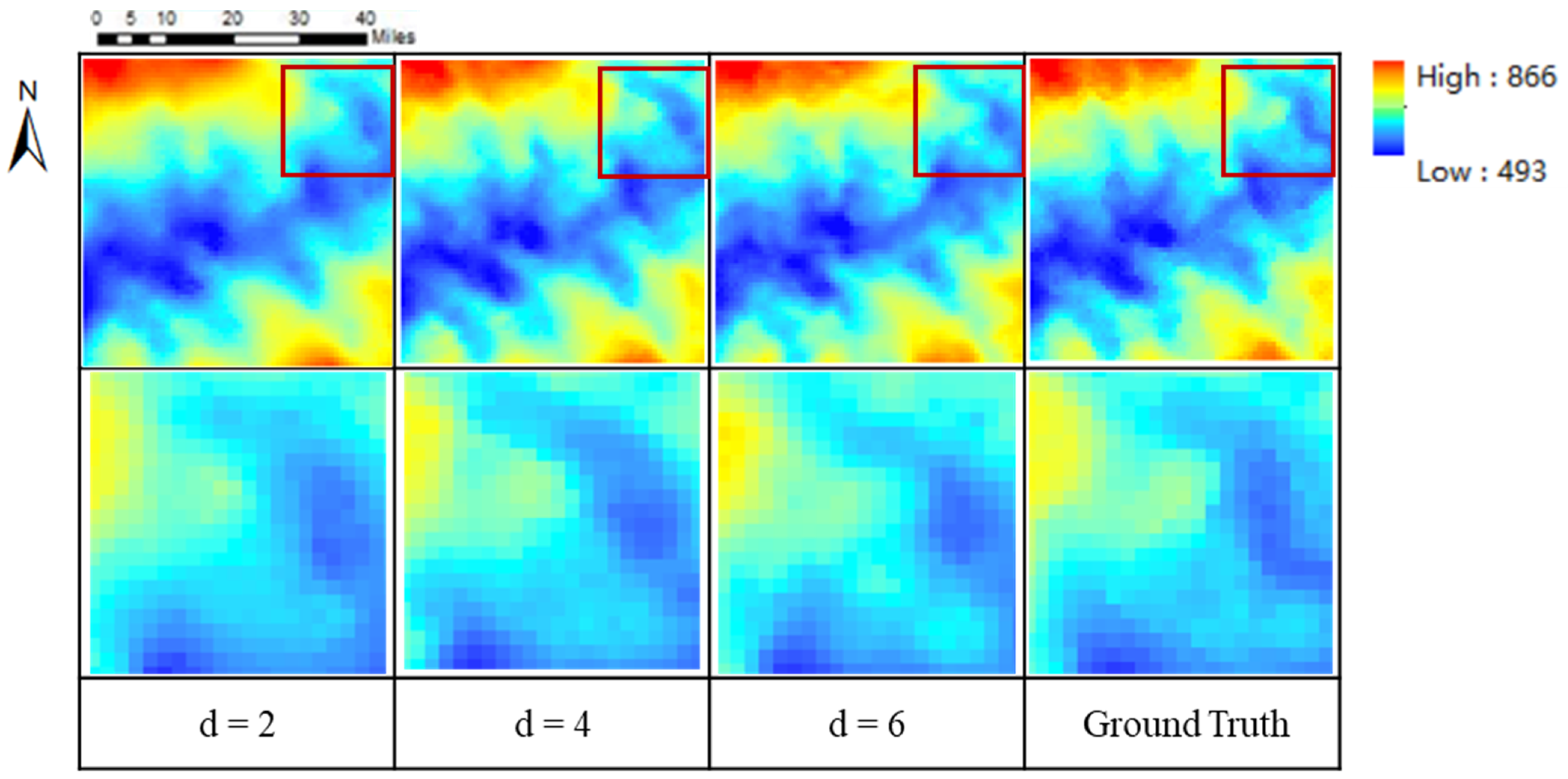
5.2.4. The Impact of the Different Down Sampling Factors

In this section, the effectiveness of our method based on the different down sampling factors d of training data is investigated. The experimental settings are the same as the experiment in Section 4.1 except for the down sampling factor d.

As shown in

Table 6. The results of DEM reconstructed with the down sampling factor d of two, four, and six.

Scale	Elevation		SSIM
	MAE	RMSE
2	4.434	5.701	0.935
4	5.702	7.333	0.913
6	7.147	8.976	0.874

and Figure 18, when d is two, the DEM reconstructed from the model is closest to the original DEM. This is because with the increase of d, the low-resolution pixel data becomes less, and more limited information is obtained. When d is six, more local features will be lost, and only the basic terrain feature contour can be reconstructed. This is because the down sampling factor is too large, and fewer known features bring great challenges to DEM reconstruction. To sum up, our GISR method can reconstruct DEMs that are very close to the ground truth under conditions that use different down sampling factors, which fully demonstrates that the GISR method can be widely used for DEM SR tasks with different down sampling factors.

5.2.5. Limitations

In the proposed GISR method, the global information supplement module is used to supplement certain transmission loss information and global information by considering spatial autocorrelation to reproduce a more realistic geographical distribution pattern. The Kriging interpolation method accounts for spatial autocorrelation, which can provide global terrain information; thus, we designed our modules based on it. In this way, the interpolation effect of the Kriging method directly affects the effectiveness of the GISR method. For some regions with complex terrain, the Kriging method will fail to interpolate; therefore, the quality of the DEM generated by our method will be greatly reduced. In our follow-up work, we will try to introduce the idea of a transformer [27] into the DEM SR process to achieve the acquisition of global information from the underlying network architecture.

6. Conclusions

This paper proposes a global-information-constrained depth learning network for digital elevation model super-resolution (GISR). The global information supplement module, which can reflect spatial autocorrelation, is designed based on the Kriging method in order to supplement some transmission loss information and global information through the consideration of spatial autocorrelation. In the test area with different terrain complexities, GISR performs well in regard to elevation accuracy and terrain maintenance compared with other classical interpolation methods (bicubic interpolation and Kriging interpolation) and deep learning networks (SRResNet, TfaSR, and SRCNN). The DEM generated by this method is closer to the real terrain, and compared with the deep learning method, the RMSE of our results is improved by 20.5% to 68.8%. The GISR method can be widely used for DEM SR tasks with different down sampling factors and has strong data adaptability.

The results show that the proposed global information supplement module based on terrain spatial autocorrelation can be embedded into other terrain generation tasks. Ultimately, our work reveals the feasibility of studying terrain models from the perspective of network transmission and information supplementation, which, to some extent, enhances the interpretability of the DEM super-resolution network and provides a new idea for completing high-precision DEM generation tasks.

References

1. Passalacqua, P.; Tarolli, P.; Foufoula-Georgiou, E. Testing space-scale methodologies for automatic geomorphic feature extraction from lidar in a complex mountainous landscape. Water Resour. Res. 2010, 46. [Google Scholar] [CrossRef] [Green Version]
2. Kenward, T.; Lettenmaier, D.P.; Wood, E.F.; Fielding, E. Effects of digital elevation model accuracy on hydrologic predictions. Remote Sens. Environ. 2000, 74, 432–444. [Google Scholar] [CrossRef]
3. Huang, C.; Chen, Y.; Wu, J. DEM-based modification of pixel-swapping algorithm for enhancing floodplain inundation mapping. Int. J. Remote Sens. 2014, 35, 365–381. [Google Scholar] [CrossRef]
4. Kellndorfer, J.; Walker, W.; Pierce, L.; Dobson, C.; Fites, J.A.; Hunsaker, C.; Vona, J.; Clutter, M. Vegetation height estimation from shuttle radar topography mission and national elevation datasets. Remote Sens. Environ. 2004, 93, 339–358. [Google Scholar] [CrossRef]
5. Chen, D.; Zhong, Y.; Zheng, Z.; Ma, A.; Lu, X. Urban road mapping based on an end-to-end road vectorization mapping network framework. ISPRS J. Photogramm. Remote Sens. 2021, 178, 345–365. [Google Scholar] [CrossRef]
6. Chen, Z.; Wang, X.; Xu, Z. Convolutional Neural Network Based Dem Super Resolution. Int. Arch. Photogramm. Remote Sens. Spat. Inf. Sci. 2016, 41, 247–250. [Google Scholar] [CrossRef] [Green Version]
7. Zhu, D.; Cheng, X.; Zhang, F.; Yao, X.; Gao, Y.; Liu, Y. Spatial interpolation using conditional generative adversarial neural networks. Int. J. Geogr. Inf. Sci. 2020, 34, 735–758. [Google Scholar] [CrossRef]
8. Han, D. Comparison of commonly used image interpolation methods. In Proceedings of the Conference of the 2nd International Conference on Computer Science and Electronics Engineering (ICCSEE 2013), Paris, France, 22–23 March 2013; pp. 1556–1559. [Google Scholar]
9. Zhang, Y.; Yu, W. Comparison of DEM Super-Resolution Methods Based on Interpolation and Neural Networks. Sensors 2022, 22, 745. [Google Scholar] [CrossRef]
10. Li, J.; Heap, A.D. A review of comparative studies of spatial interpolation methods in environmental sciences: Performance and impact factors. Ecol. Inform. 2011, 6, 228–241. [Google Scholar] [CrossRef]
11. LeCun, Y.; Bengio, Y.; Hinton, G. Deep learning. Nature 2015, 521, 436–444. [Google Scholar] [CrossRef]
12. Musakwa, W.; Van Niekerk, A. Monitoring urban sprawl and sustainable urban development using the Moran Index: A case study of Stellenbosch, South Africa. Int. J. Appl. Geospat. Res. (IJAGR) 2014, 5, 1–20. [Google Scholar] [CrossRef] [Green Version]
13. Zhou, A.; Chen, Y.; Wilson, J.P.; Su, H.; Xiong, Z.; Cheng, Q. An Enhanced Double-Filter Deep Residual Neural Network for Generating Super Resolution DEMs. Remote Sens. 2021, 13, 3089. [Google Scholar] [CrossRef]
14. Knudsen, E.I. Fundamental components of attention. Annu. Rev. Neurosci. 2007, 30, 57–78. [Google Scholar] [CrossRef]
15. Shaw, P.; Uszkoreit, J.; Vaswani, A. Self-attention with relative position representations. arXiv 2018, arXiv:1803.02155. [Google Scholar]
16. Pashler, H.; Johnston, J.C.; Ruthruff, E. Attention and performance. Annu. Rev. Psychol. 2001, 52, 629. [Google Scholar] [CrossRef] [Green Version]
17. Demiray, B.Z.; Sit, M.; Demir, I. D-SRGAN: DEM super-resolution with generative adversarial networks. SN Comput. Sci. 2021, 2, 48. [Google Scholar] [CrossRef]
18. Getis, A. Spatial autocorrelation. In Handbook of Applied Spatial Analysis; Springer: Berlin/Heidelberg, Germany, 2010; pp. 255–278. [Google Scholar]
19. Chen, T.-J.; Chuang, K.-S.; Wu, J.; Chen, S.C.; Hwang, M.; Jan, M.-L. A novel image quality index using Moran I statistics. Phys. Med. Biol. 2003, 48, N131. [Google Scholar] [CrossRef]
20. Kattenborn, T.; Leitloff, J.; Schiefer, F.; Hinz, S. Review on Convolutional Neural Networks (CNN) in vegetation remote sensing. ISPRS J. Photogramm. Remote Sens. 2021, 173, 24–49. [Google Scholar] [CrossRef]
21. Alzubaidi, L.; Zhang, J.; Humaidi, A.J.; Al-Dujaili, A.; Duan, Y.; Al-Shamma, O.; Santamaría, J.; Fadhel, M.A.; Al-Amidie, M.; Farhan, L. Review of deep learning: Concepts, CNN architectures, challenges, applications, future directions. J. Big Data 2021, 8, 53. [Google Scholar] [CrossRef]
22. Targ, S.; Almeida, D.; Lyman, K. Resnet in resnet: Generalizing residual architectures. arXiv 2016, arXiv:1603.08029. [Google Scholar]
23. He, K.; Zhang, X.; Ren, S.; Sun, J. Deep residual learning for image recognition. In Proceedings of the IEEE Conference on Computer Vision and Pattern Recognition, Seattle, WA, USA, 17–19 June 2016; pp. 770–778. [Google Scholar]
24. Shi, W.; Caballero, J.; Huszár, F.; Totz, J.; Aitken, A.P.; Bishop, R.; Rueckert, D.; Wang, Z. Real-time single image and video super-resolution using an efficient sub-pixel convolutional neural network. In Proceedings of the IEEE Conference on Computer Vision and Pattern Recognition, Seattle, WA, USA, 17–19 June 2016; pp. 1874–1883. [Google Scholar]
25. Dai, J.; Qi, H.; Xiong, Y.; Li, Y.; Zhang, G.; Hu, H.; Wei, Y. Deformable convolutional networks. In Proceedings of the IEEE International Conference on Computer Vision, Seoul, Republic of Korea, 20–23 June 2017; pp. 764–773. [Google Scholar]
26. Thomas, H.; Qi, C.R.; Deschaud, J.-E.; Marcotegui, B.; Goulette, F.; Guibas, L.J. Kpconv: Flexible and deformable convolution for point clouds. In Proceedings of the IEEE/CVF International Conference on Computer Vision, Montreal, BC, Canada, 17 October 2019; pp. 6411–6420. [Google Scholar]
27. Han, K.; Xiao, A.; Wu, E.; Guo, J.; Xu, C.; Wang, Y. Transformer in transformer. Adv. Neural Inf. Process. Syst. 2021, 34, 15908–15919. [Google Scholar]
28. Parmar, N.; Vaswani, A.; Uszkoreit, J.; Kaiser, L.; Shazeer, N.; Ku, A.; Tran, D. Image transformer. In Proceedings of the International Conference on Machine Learning, Baltimore, MD, USA, 17–23 July 2018; pp. 4055–4064. [Google Scholar]
29. Vaswani, A.; Shazeer, N.; Parmar, N.; Uszkoreit, J.; Jones, L.; Gomez, A.N.; Kaiser, Ł.; Polosukhin, I. Attention is all you need. In Proceedings of the Annual Conference on Neural Information Processing Systems, Long Beach, CA, USA, 4–9 December 2017; 30. [Google Scholar]
30. Cressie, N. The origins of kriging. Math. Geol. 1990, 22, 239–252. [Google Scholar] [CrossRef]
31. Zhang, Y.; Yu, W.; Zhu, D. Terrain feature-aware deep learning network for digital elevation model superresolution. ISPRS J. Photogramm. Remote Sens. 2022, 189, 143–162. [Google Scholar] [CrossRef]
32. Ledig, C.; Theis, L.; Huszár, F.; Caballero, J.; Cunningham, A.; Acosta, A.; Aitken, A.; Tejani, A.; Totz, J.; Wang, Z. Photo-realistic single image super-resolution using a generative adversarial network. In Proceedings of the IEEE Conference on Computer Vision and Pattern Recognition, Seattle, WA, USA, 18–22 June 2017; pp. 4681–4690. [Google Scholar]
33. Dong, C.; Loy, C.C.; He, K.; Tang, X. Image super-resolution using deep convolutional networks. IEEE Trans. Pattern Anal. Mach. Intell. 2015, 38, 295–307. [Google Scholar] [CrossRef] [PubMed] [Green Version]
34. Atkinson, P.M.; Lloyd, C.D. Geostatistics and spatial interpolation. In The SAGE Handbook of Spatial Analysis; SAGE: Newcastle upon Tyne, UK, 2009; pp. 159–181. [Google Scholar]
35. Shepard, D. A two-dimensional interpolation function for irregularly-spaced data. In Proceedings of the 1968 23rd ACM National Conference, New York, NY, USA, 27–29 August 1968; pp. 517–524. [Google Scholar]
36. Taunk, K.; De, S.; Verma, S.; Swetapadma, A. A brief review of nearest neighbor algorithm for learning and classification. In Proceedings of the 2019 International Conference on Intelligent Computing and Control Systems (ICCS), Madurai, India, 15–17 May 2019; pp. 1255–1260. [Google Scholar]
37. Bhatia, N. Survey of nearest neighbor techniques. arXiv 2010, arXiv:1007.0085. [Google Scholar]
38. McKinley, S.; Levine, M. Cubic spline interpolation. Coll. Redw. 1998, 45, 1049–1060. [Google Scholar]
39. Wahba, G. Spline interpolation and smoothing on the sphere. SIAM J. Sci. Stat. Comput. 1981, 2, 5–16. [Google Scholar] [CrossRef]
40. Gao, S.; Gruev, V. Bilinear and bicubic interpolation methods for division of focal plane polarimeters. Opt. Express 2011, 19, 26161–26173. [Google Scholar] [CrossRef]
41. De Boor, C. Bicubic spline interpolation. J. Math. Phys. 1962, 41, 212–218. [Google Scholar] [CrossRef]
42. Wackernagel, H. Ordinary kriging. In Multivariate Geostatistics; Springer: Berlin/Heidelberg, Germany, 2003; pp. 79–88. [Google Scholar]
43. Hutchinson, M.; Gessler, P. Splines—More than just a smooth interpolator. Geoderma 1994, 62, 45–67. [Google Scholar] [CrossRef]
44. Sun, M.; Song, Z.; Jiang, X.; Pan, J.; Pang, Y. Learning pooling for convolutional neural network. Neurocomputing 2017, 224, 96–104. [Google Scholar] [CrossRef]
45. Yu, D.; Wang, H.; Chen, P.; Wei, Z. Mixed pooling for convolutional neural networks. In Proceedings of the International Conference on Rough Sets and Knowledge Yechnology, Shanghai, China, 24–26 October 2014; pp. 364–375. [Google Scholar]
46. Tang, J.; Xia, H.; Zhang, J.; Qiao, J.; Yu, W. Deep forest regression based on cross-layer full connection. Neural Comput. Appl. 2021, 33, 9307–9328. [Google Scholar] [CrossRef]
47. Boutell, M.R.; Luo, J.; Shen, X.; Brown, C.M. Learning multi-label scene classification. Pattern Recognit. 2004, 37, 1757–1771. [Google Scholar] [CrossRef] [Green Version]
48. Cheng, G.; Han, J.; Lu, X. Remote sensing image scene classification: Benchmark and state of the art. Proc. IEEE 2017, 105, 1865–1883. [Google Scholar] [CrossRef] [Green Version]
49. Noh, H.; Hong, S.; Han, B. Learning deconvolution network for semantic segmentation. In Proceedings of the IEEE International Conference on Computer Vision, Beijing, China, 17–21 October 2015; pp. 1520–1528. [Google Scholar]
50. Zhao, Z.-Q.; Zheng, P.; Xu, S.-t.; Wu, X. Object detection with deep learning: A review. IEEE Trans. Neural Netw. Learn. Syst. 2019, 30, 3212–3232. [Google Scholar] [CrossRef]
51. Zou, Z.; Shi, Z.; Guo, Y.; Ye, J. Object detection in 20 years: A survey. arXiv 2019, arXiv:1905.05055. [Google Scholar]
52. Long, J.; Shelhamer, E.; Darrell, T. Fully convolutional networks for semantic segmentation. In Proceedings of the IEEE Conference on Computer Vision and Pattern Recognition, Seattle, WA, USA, 19 June 2015; pp. 3431–3440. [Google Scholar]
53. He, K.; Zhang, X.; Ren, S.; Sun, J. Delving deep into rectifiers: Surpassing human-level performance on imagenet classification. In Proceedings of the IEEE International Conference on Computer Vision, Beijing, China, 17–21 October 2015; pp. 1026–1034. [Google Scholar]
54. Demiray, B.Z.; Sit, M.; Demir, I. DEM Super-Resolution with EfficientNetV2. arXiv 2021, arXiv:2109.09661. [Google Scholar]
55. Lin, X.; Zhang, Q.; Wang, H.; Yao, C.; Chen, C.; Cheng, L.; Li, Z. A DEM Super-Resolution Reconstruction Network Combining Internal and External Learning. Remote Sens. 2022, 14, 2181. [Google Scholar] [CrossRef]
56. Zhang, R.; Bian, S.; Li, H. RSPCN: Super-Resolution of Digital Elevation Model Based on Recursive Sub-Pixel Convolutional Neural Networks. ISPRS Int. J. Geo-Inf. 2021, 10, 501. [Google Scholar] [CrossRef]
57. He, P.; Cheng, Y.; Qi, M.; Cao, Z.; Zhang, H.; Ma, S.; Yao, S.; Wang, Q. Super-Resolution of Digital Elevation Model with Local Implicit Function Representation. In Proceedings of the 2022 International Conference on Machine Learning and Intelligent Systems Engineering (MLISE), Seoul, Korea, 8–11 November 2022; pp. 111–116. [Google Scholar]
58. Koenig, W.D. Spatial autocorrelation of ecological phenomena. Trends Ecol. Evol. 1999, 14, 22–26. [Google Scholar] [CrossRef] [PubMed]
59. Ioffe, S.; Szegedy, C. Batch normalization: Accelerating deep network training by reducing internal covariate shift. In Proceedings of the International Conference on Machine Learning, Baltimore, MD, USA, 17–23 July 2015; pp. 448–456. [Google Scholar]
60. Fan, E. Extended tanh-function method and its applications to nonlinear equations. Phys. Lett. A 2000, 277, 212–218. [Google Scholar] [CrossRef]
61. Maas, A.L.; Hannun, A.Y.; Ng, A.Y. Rectifier nonlinearities improve neural network acoustic models. In Proceedings of the 30th International Conference on Machine Learning 2013, Atlanta, GA, USA, 16–21 June 2013; p. 3. [Google Scholar]
62. Nair, V.; Hinton, G.E. Rectified linear units improve restricted boltzmann machines. In Proceedings of the International Conference on Machine Learning, Haifa, Israel, 21–24 June 2010. [Google Scholar]
63. Glorot, X.; Bengio, Y. Understanding the difficulty of training deep feedforward neural networks. In Proceedings of the Thirteenth International Conference on Artificial Intelligence and Statistics, 2010, Sardinia, Italy, 13–15 May 2010; pp. 249–256. [Google Scholar]
64. Simonyan, K.; Zisserman, A. Very deep convolutional networks for large-scale image recognition. arXiv 2014, arXiv:1409.1556. [Google Scholar]
65. Kingma, D.P.; Ba, J. Adam: A method for stochastic optimization. arXiv 2014, arXiv:1412.6980. [Google Scholar]
66. Bolstad, P.V.; Stowe, T. An evaluation of DEM accuracy: Elevation, slope, and aspect. Photogramm. Eng. Remote Sens. 1994, 60, 1327–1332. [Google Scholar]
67. Wang, S.; Rehman, A.; Wang, Z.; Ma, S.; Gao, W. SSIM-motivated rate-distortion optimization for video coding. IEEE Trans. Circuits Syst. Video Technol. 2011, 22, 516–529. [Google Scholar] [CrossRef] [Green Version]
68. Chai, T.; Draxler, R.R. Root mean square error (RMSE) or mean absolute error (MAE)?–Arguments against avoiding RMSE in the literature. Geosci. Model Dev. 2014, 7, 1247–1250. [Google Scholar] [CrossRef]
Figure 1. The elevation values of the terrain have spatial correlation: (a) is the remote sensing images of the region, (b) is the DEM of the region, and (c) is the LISA (local indicators of spatial association) map.
Remotesensing 15 00305 g001
Figure 2. Overview of the proposed global-information-constrained deep learning network for generating super-resolution DEMs (GISR).
Remotesensing 15 00305 g002
Figure 3. Process steps of Kriging interpolation (the left input is low-resolution DEM, and the right output is interpolated high-resolution DEM).
Remotesensing 15 00305 g003
Figure 4. The details of residual feature extraction module (Conv 3 × 3 is convolution layer with kernel size = 3).
Remotesensing 15 00305 g004
Figure 5. The process of sampling DEM with PixelShuffle: (a) is the input 6 × 6 low-resolution DEM, (b) is the r 2 feature maps extracted from subgraph, and (c) is the 12 × 12 high-resolution result after up sampling.
Remotesensing 15 00305 g005
Figure 6. Study area and its elevation and slope parameters: (a) is the DEM of the study area, (b) is the elevation distribution of the study area, and (c) is the slope distribution of the study area.
Remotesensing 15 00305 g006
Figure 7. Detailed DEM parameters for each of the four test regions: (a) is the DEM of the study region, (b) is the elevation distribution of the study region, (c) is the elevation drop in the vertical direction of the study region, (d) is the statistics of elevation drop in the vertical direction of the study region, (e) is the slope distribution of the study region, (f) is the statistics slope distribution of the study region, (g) is the elevation drop in the horizontal direction of the study region, and (h) is the statistics of elevation drop in the horizontal direction of the study region. The horizontal direction is the elevation difference between the left and right adjacent pixels, and the vertical direction is the elevation difference between the up and down adjacent pixels.
Remotesensing 15 00305 g007
Figure 8. Training details of the GISR method.
Remotesensing 15 00305 g008
Figure 9. Unsatisfactory interpolation sample.
Remotesensing 15 00305 g009
Figure 10. The performance of the proposed GISR during the training process using DEM data (The contents of the solid wireframe are the enlarged details of the dotted wireframe).
Remotesensing 15 00305 g010
Figure 11. The DEM SR results of different methods in four test regions: (ad) are the test regions R1, R2, R3, and R4, respectively (The contents of the solid wireframe are the enlarged details of the dotted wireframe).
Remotesensing 15 00305 g011
Figure 12. The DEM SR slope results for four different methods: (ad) are the test regions R1, R2, R3, and R4, respectively (The contents of the solid wireframe are the enlarged details of the dotted wireframe).
Remotesensing 15 00305 g012
Figure 13. Visualization results of the role of different modules: (a) is the DEM SR result, and (b) is the DEM SR slope (RG-GISR means the global information supplement module was removed; The details in the red box are in the next row).
Remotesensing 15 00305 g013
Figure 14. Global information supplement: (a) is the DEM has global information supplement, (b) is the DEM has not global information, and (c) is the ground truth (The details in the red box are in the next row).
Remotesensing 15 00305 g014
Figure 15. Results of different loss schemes: (a) is the DEM SR result, and (b) is the DEM SR slope(The details in the red box are in the next row).
Remotesensing 15 00305 g015
Figure 16. DEM and slope of our method (GISR) with different parameter settings.
Remotesensing 15 00305 g016
Figure 17. Results of different DEM SR methods on TfaSR dataset (The details in the red box are in the next row).
Remotesensing 15 00305 g017
Figure 18. DEM SR results for different down sampling factors (The details in the red box are in the next row).
Remotesensing 15 00305 g018