Low-Rank Constrained Attention-Enhanced Multiple Spatial–Spectral Feature Fusion for Small Sample Hyperspectral Image Classification

Abstract

Hyperspectral images contain rich features in both spectral and spatial domains, which bring opportunities for accurate recognition of similar materials and promote various fine-grained remote sensing applications. Although deep learning models have been extensively investigated in the field of hyperspectral image classification (HSIC) tasks, classification performance is still limited under small sample conditions, and this has been a longstanding problem. The features extracted by complex network structures with large model size are redundant to some extent and prone to overfitting. This paper proposes a low-rank constrained attention-enhanced multiple feature fusion network (LAMFN). Firstly, factor analysis is used to extract very few components that can describe the original data using covariance information to perform spectral feature preprocessing. Then, a lightweight attention-enhanced 3D convolution module is used for deep feature extraction, and the position-sensitive information is supplemented using a 2D coordinate attention. The above widely varying spatial–spectral feature groups are fused through a simple composite residual structure. Finally, low-rank second-order pooling is adopted to enhance the convolutional feature selectivity and achieve classification. Extensive experiments were conducted on four representative hyperspectral datasets with different spatial–spectral characteristics, namely Indian Pines (IP), Pavia Center (PC), Houston (HU), and WHU-HongHu (WHU). The contrast methods include several advanced models proposed recently, including residual CNNs, attention-based CNNs, and transformer-based models. Using only five samples per class for training, LAMFN achieved overall accuracies of 78.15%, 97.18%, 81.35%, and 87.93% on the above datasets, which has an improvement of 0.82%, 1.12%, 1.67%, and 0.89% compared to the second-best model. The running time of LAMFN is moderate. For example, the training time of LAMFN on the WHU dataset was 29.1 s, and the contrast models ranged from 3.0 s to 341.4 s. In addition, ablation experiments and comparisons with some advanced semi-supervised learning methods further validated the effectiveness of the proposed model designs.

1. Introduction

Hyperspectral images (HSI) exhibit rich features in the 2D spatial context domain and the 1D spectral reflectance domain, which support accurate recognition of objects with similar colors and textures. With the rapid development of portable sensors and unmanned aerial vehicle (UAV) remote sensing platforms, the acquired hyperspectral images show remarkable characteristics of high spatial resolution, which further promote precision agriculture, environmental monitoring, forestry, and other fields [1,2,3]. Therefore, hyperspectral image classification (HSIC) is the cornerstone of many fine-grained remote sensing applications and has received continued attention. However, the fine-grained classification of HSI still needs to be improved due to inherent data complexity and small sample dilemma.

HSIC research spans several decades, and some consensus has been developed on the difficulties of accurate classification. First, feature extraction and representation are the core steps since hyperspectral data share high dimensionality and high nonlinearity [4]. Prior to the dense usage of deep learning methods, HSIC research focused on well-designed features and machine learning classifiers. Secondly, the artificial fusion of multi-types of features effectively improves classification accuracy. Introducing spatial contextual information for an individual pixel can enhance the richness of spatial–spectral features and boost classification accuracy [5,6]. Finally, hyperspectral data annotation is time-consuming and laborious, thus HSIC encounters the significant small sample dilemma [7]. In addition, to cope with high data redundancy, dimensionality reduction (DR) methods have raised considerable concern and become popular feature extraction methods and pre-processing steps [8]. Principal component analysis (PCA) and its variants, such as kernel principal component analysis (KPCA), are such traditional DR methods that can filter data redundancy in the spectral domain [9]. Recently, novel spatial–spectral DR methods have been paid considerable attention [10,11]. Focusing on the specific high dimensional data structure, manifold learning-based methods are also investigated to evolve spatial correlation in the DR process [12]. Shi et al. proposed spatial–spectral multiple manifold discriminant analysis (SSMMDA) for DR in HSIC tasks, and the multi-manifold structure of HSI data has been elaborately considered [13]. The above consensus, namely multi-feature fusion, spatial–spectral joint feature extraction, and various DR methods, are seen as crucial prior knowledge for HSIC tasks. Due to sufficient experimental verification or a solid theoretical basis, the above multiple prior knowledge plays an essential role in the HSIC tasks, which will always be a research hotspot.

Deep learning methods are extensively investigated for HSIC due to their ability to extract abstract and robust features in a data-driven manner, which can obtain better classification performance than traditional methods [14]. CNN is one of the mainstream methods for HSIC due to its inherent applicability to 3D data structures. Continuous, in-depth and extensive research on CNN-based hyperspectral classification has been performed, in which 2D-CNN and 3D-CNN are commonly used models for HSIC [15,16,17,18,19]. In particular, 2D-CNN focuses on learning spatial features, while 3D-CNN has a good pertinency for hyperspectral data cube [20]. Roy et al. proposed a hybrid convolutional network (HybridSN) by fusing 3D-CNN and 2D-CNN, which effectively combines the advantages of both types of networks [21]. Building on 3D-CNN and 3D-2D-CNN, residual learning and dense connections have been investigated to optimize the network structure and boost the feature robustness [22,23]. Song et al. proposed cross-layer feature aggregation in a 2D residual network and verified the effectiveness of composite residual structure for hyperspectral classification [24]. Feng et al. proposed R-HybridSN, which uses residual connections to fuse different scales and different types of features and introduces depth-separable convolutions to significantly reduce the number of parameters [25]. Although deep 3D-CNNs can learn robust features with sufficient training data, they still suffer from overfitting problems in small sample conditions. Meanwhile, feature redundancy and limited perceptual fields are inherent limitations of 3D-CNN models in real-world small sample HSIC tasks.

To address the inherent limitations of deep CNN models, the visual attention mechanism was introduced for convolutional feature refinement. Visual attention is a network resource allocation mechanism that allows the network to focus more on features that are useful for classification through adaptive weight assignment [26]. Attention-based models, as a rising network paradigm, have developed gradually deeper integration with CNN models and received much attention in HSIC [27]. Mou et al. introduced spectral attention to hyperspectral data before feeding them into the CNN model. Band-wise adaptive calibration has been performed to improve classification accuracy and model interpretability [28]. Zhu et al. applied spectral–spatial attention to both raw hyperspectral data and residual modules in the network, which expanded the form of the convolution-attention fusion pattern and improved the robustness of spatial–spectral features [29]. Zhang et al. proposed the attention-dense hybrid convolutional network (AD-HybridSN), which introduces channel attention after each 3D convolution layer and spatial attention after each 2D convolution layer to achieve layer-wise spatial–spectral feature refinement [30]. Dong et al. designed cooperative spectral–spatial attention based on parallel learning of spatial weights and spectral weights and enhanced the feature expression ability of attention modules with dense connections [31]. To sum up, the integration of attention modules with CNN models has experienced three stages, namely simple embedding, stage-wise fusion, and layer-wise fusion. In addition, attention modules can also be directly used for spatial–spectral feature extraction [32,33].

Unlike convolution-attention fusion models, Transformer is a representative pure attention paradigm that learns global features by stacking self-attention modules. Vision transformer (VIT) has achieved comparable results with advanced CNN in various image processing tasks [34]. Recently, transformer-based models have been primarily explored in HSIC tacks, with a focus on specific data organization and feature fusion patterns. Hong et al. proposed spectral-former based on VIT. The group-wise embedding was adopted to strengthen the neighborhood spectral feature learning, and the cross-layer adaptive fusion module was used to enhance the feature interaction level [35]. Sun et al. proposed SSFTT by integrating 3D convolution, 2D convolution, and self-attention modules, in which the features extracted from the convolution layer were used as the prior knowledge for the self-attention layers [36]. Xue et al. introduced spatial partition restore (SPR) in local transformer to ensure pixel constraints, which strengthened local spatial dependency [37]. Although transformer-based models can obtain comparable results with advanced CNN models using sufficient training samples, they usually take longer time to fit the data. Meanwhile, transformer-based models pay more attention to global feature learning, which often leads to a large parameter number and overfitting in the small sample classification tasks. The transformer-based models may be further improved by drawing on some of the properties of CNNs.

The CNN models are seen as multi-layer local feature learning frameworks, and they are also benefiting from global feature learning ideas, such as large kernels and graph learning. First, the inherent limitations have been enhanced with redesigned models featuring large convolutional kernels and elegant structures, such as ConvNeXt and RepLKNet [38,39]. Second, graph CNN (GCN) has been proposed to combine graph learning with CNN to learn long-range features. Recently, Zhu et al. proposed a multi-scale short- and long-range graph convolutional network (MSLGCN) for HSIC. Multi-scale spatial embeddings and global spectral features are deeply explored by an elegant multi-stage structure [40]. Third, holistic image representation can be better learned by collecting second-order statistics of convolutional features. Feng et al. extracted spatial–spectral features using factor analysis and a cascade feature fusion architecture with parallel convolutional kernels of different sizes. Second-order pooling and L2 normalization are utilized to exploit the higher-order statistics of features extracted by CNN models [41]. In addition, the underlying convolution operation is being revisited and improved. Roy et al. designed a generalized gradient-centered 3D convolution, improving the feature learning power for HSI from the gradient level [42].

Unsupervised feature learning methods have a good reputation as they are impressive solutions to small sample HSIC tasks. The core idea of unsupervised learning is to construct additional supervised signals and evolve unlabeled data in the training process [43]. Zhu et al. proposed a self-supervised contrastive efficient asymmetric dilated network (SC-EADNet) and performed contrastive learning with the help of random crop augmentation [44]. Liu et al. proposed multi-view unsupervised contrastive learning framework using different PCA-reduced band intervals as contrastive sample pairs [45]. Facing cross-domain small sample HSIC tasks, Liu et al. proposed deep few-shot learning (DFSL) [46]. The deep residual network is used to learn a metric space in pre-collected datasets, and then a very small number of samples (five for each class) from the target domain are used for feature extraction and classification separately. Gao et al. proposed an end-to-end deep relation network-based few-shot classification (RN-FSC) framework, which can be seen as an improved version of DFSL [47]. Recently, an unsupervised metric learning framework with multi-view constraints was proposed and further promoted cross-domain HSIC tasks [48]. Most of the above methods are pioneering works that have normalized the hyperspectral un-supervised learning paradigm to some extent. However, there are still some shortcomings. For example, unsupervised learning with only several bands does not excavate the spectral features well in DFSL and RN-FSC. In addition, there is a lack of research on the applicability of model structure and unsupervised learning.

Facing the difficulties in fine-grained small sample hyperspectral classification, a framework based on low-rank constrained attention-enhanced multiple spatial–spectral feature fusion was designed in this paper. The aim of our research is to simplify the existing complex models, find out useful features with low redundancy, and make the best use of the extracted spatial–spectral embeddings. The proposed framework and main contributions are summarized as follows:

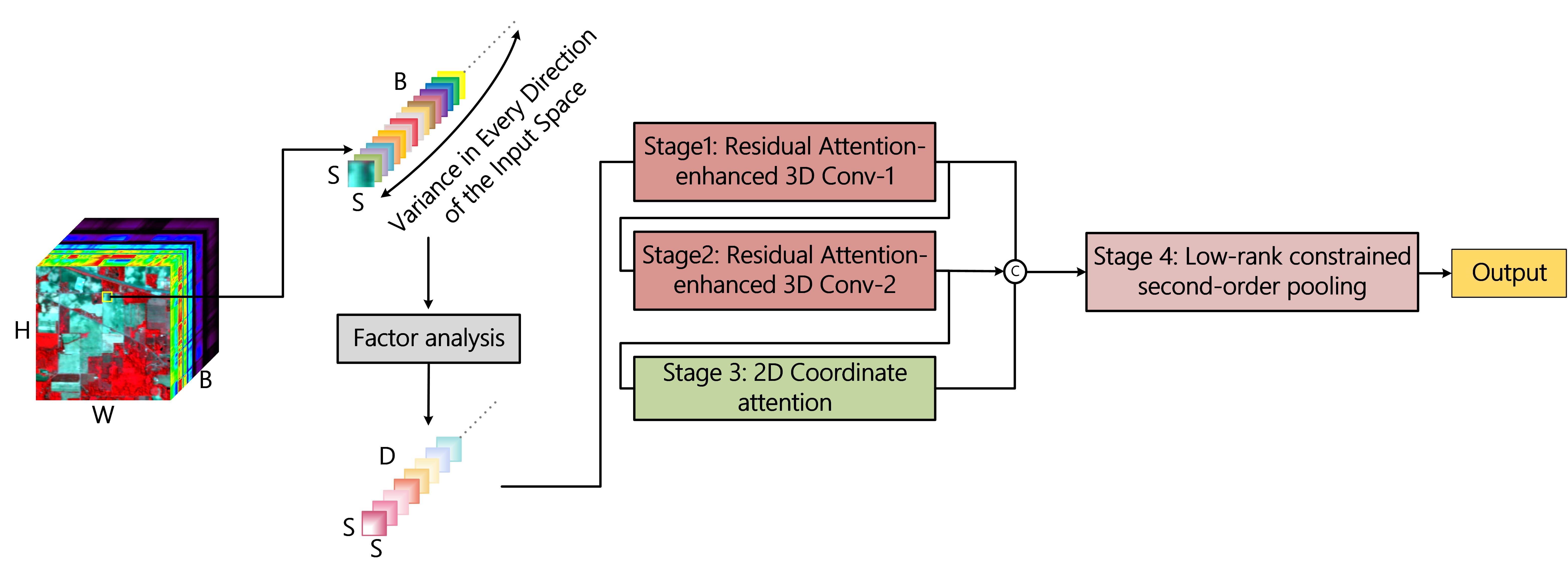
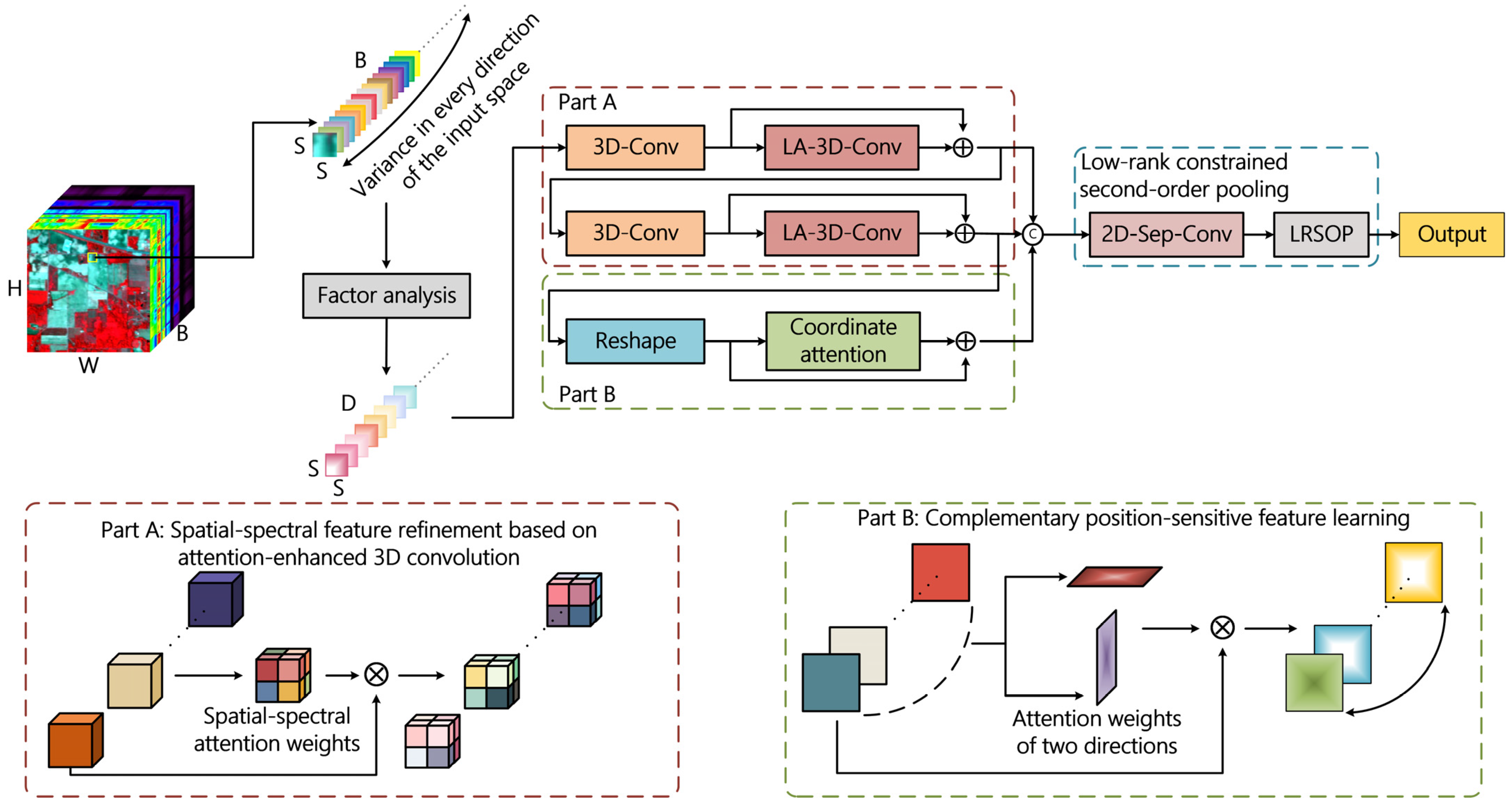
• To fit the small sample dilemma, a few components that can model the hyperspectral data are first extracted using factor analysis to reduce data redundancy. One single vanilla 3D convolutional layer is utilized to primarily investigate spatial–spectral features, and the features are then further refined based on an attention-like manner.
• Complementary position-sensitive and channel correlation information are provided by coordinate attention. The multi-level features extracted by 3D convolution and 2D attention are then unified and aggregated by a simple and effective composite residual structure. Finally, a compact vector of second-order statistics is learned for each class using low-rank second-order pooling to achieve classification.
• Extensive experiments have been performed using four representative hyperspectral datasets with varying spatial–spectral characteristics. Using only five samples of each class for training, the LAMFN outperforms several recently released well-designed models with smaller parameter size and shorter running time.

2. Related Research

2.1. Mixed CNN Model

2D convolution is a commonly used feature extraction operator for RGB images. Assuming that the input feature dimension is $H\times W\times B$ and the padding strategy is used, the output dimension of $p$ 2D convolution kernels will be $H\times W\times p$. Obviously, the features extracted by each 2D convolution kernel can be regarded as a weighted average of the $B$ channel features [15]. This manner leads to spectral feature loss and can only highlight the contributions of different bands using multiple convolution kernels. In contrast, 3D convolution extends explicit feature extraction to the spectral domain in HSIC tasks. The $p$ 3D convolutional kernel will output $H\times W\times B\times p$ feature maps, and each 3D kernel convolves the input data from three directions [20]. However, when using an equal number of kernels, the required computational resources by 3D convolution are much larger than that of 2D convolution. The complexity increase is particularly noticeable when large kernel sizes are adopted, such as $7\times 7\times 7$.

The single-type CNN models can be improved by using a combination of 3D convolution and 2D convolution to form a mixed CNN model [25,30,41]. The basic structure of a mixed convolutional network can be divided into four basic building blocks, namely, 3D convolution, reshape, 2D convolution, and fully connected layers [21]. The 3D convolutional layer learns the spatial–spectral features, and the output dimension is $H\times W\times B\times C$, where $C$ is the number of 3D kernels. It should be noted that spectral features will be preserved and integrated during the 3D convolution process. The reshape operation reorganizes the four-dimensional tensor into a three-dimensional tensor with dimensions $H\times W\times BC$, which greatly enhances the spectral feature discriminability. The 2D convolution further learns spatial features, and a fully connected layer is utilized for classification.

Although the mixed CNN model is a new feature extraction paradigm, its basic structure has some shortcomings. First, this basic structure is shallow, and the classification accuracy significantly degrades when simply increasing the number of CNN layers [18]. Second, the contribution of multi-type convolutional features to the final classification has not been fully considered. Third, the reshape operation leads to excessive channel number and feature redundancy. The above problems will be fully considered and investigated in this paper, and the corresponding solutions will be described in Section 3.

2.2. Attention Mechanism

The attention mechanism is a method designed to adaptively refine the learned features by various backbone networks in a data-driven manner and is now widely used in many remote sensing image processing tasks [27]. The basic form of the attention mechanism can be represented by Equation (1):

$$Attention\left(x\right)=f\left(g\left(x\right),x\right)$$

(1)

where $x$ denotes the input features; $g()$ is a function that calculates the weights based on the input features $x$; and $f()$ represents a function that uses the weights to refine the input features. According to the processed dimension, attention methods can be broadly classified as spatial attention, channel attention, and spatial-channel mixed attention [26]. Hyperspectral features extracted by 3D-CNN contain rich spatial and spectral information, so multiple attention mechanisms can theoretically be used to calibrate which features are more valuable for classification.

Feature adaptive selection is commonly performed by attention methods such as squeeze-and-excitation attention (SE) and convolutional block attention module (CBAM). SE is a pioneer channel attention method, and the proposed pooling-fully connected paradigm is widely used and further improved to efficiently learn feature channel weights [49]. Squeeze-and-excitation attention can be calculated using Equations (2) and (3):

$$g\left(x\right)=F{C}_e\left(F{C}_s\left(GA{P}_{spa}\left(x\right)\right)\right)$$

(2)

$$SE\left(x\right)=g\left(x\right)x$$

(3)

where $F{C}_e$ and $F{C}_s$ denote the fully connected layers used to compress and restore the channel-wise features, respectively; $GA{P}_{spa}$ represents the global average pooling, which is performed on the spatial domain. CBAM extends the SE with spatial attention, learning spatial weights using a $7\times 7$ convolution and using sequential two attentions to achieve feature refinement [50]. SE and CBAM, as classical attention methods, regulate the basic attentional form to some extent. Many improved attention methods since then can be seen as variants or combinations of SE and CBAM.

Since the receptive field of a single convolutional layer is limited, attention mechanisms can compensate for the lack of spatial–spectral features by learning global features of a particular dimension through fully connected layers. In addition, attention and convolution are often fused with residual structures for end-to-end training [51]. In our proposed model, the attention-enhanced spatial–spectral features will be extracted in a lightweight manner. And the complementary position-aware information will be considered and evolved in the mixed CNN model.

3. Methods

3.1. Network Structure

The hyperspectral classification framework, LAMFN, proposed in this paper is shown in Figure 1. First, factor analysis is performed to conduct feature transformation and extract a small number of components that can describe the hyperspectral data in terms of feature covariance. Second, the joint spatial–spectral features are extracted using two 3D convolutional layers. Meanwhile, the features are refined in a lightweight attention-enhanced manner (denoted as LA-3D-Conv in Figure 1). Third, the position-sensitive and direction-aware information are learned using a 2D coordinate attention module. Then, a multi-stage feature fusion strategy is adopted through a composite residual structure. One 2D depth separable convolution layer (2D-Sep-Conv) is adopted to integrate the multi-stage fusion features. Finally, a compact class vector is learned for each class using low-rank second-order pooling for final classification.

The classification process of the proposed framework consists of three parts: data pre-processing, spatial–spectral feature learning, and convolutional feature post-processing. The effective fusion of multi-type features with sufficient variance and low redundancy is the key to the proposed LAMFN. The vanilla 3D convolution layers are used to build a 4D spatial–spectral feature space. The LA-3D-Conv modules are designed to further integrate the learned features and improve the receptive field. The 3D spatial–spectral features with a large number of channels can be obtained by reshape operation. The 2D coordinate attention is used to investigate the unconsidered latent in 3D convolution, namely position-aware information and cross-channel correlation. Based on the effective fusion of multi-type features, the 2D-Sep-Conv and LRSOP can learn a holistic image representation.

The parameter settings for each module in LAMFN are shown in

Table 1. The implementation details of LAMFN.

	Module	Output Shape	Kernel Size	Filters or Other Parameter
Input		(15, 15, 16, 1)
Stage 1: Spatial–spectral feature learning	3D-Conv-BN-Relu	(15, 15, 16, 16)	(3, 3, 3)	16
	LA-3D-Conv	(15, 15, 16, 16)	(7, 7, 1) × 2 (1, 1, 1) × 1	16 × 2 1
	Residual structure and BN layer	(15, 15, 16, 16)
Stage 2: Spatial–spectral feature learning	3D-Conv-BN-Relu	(15, 15, 16, 16)	(3, 3, 3)	16
	LA-3D-Conv	(15, 15, 16, 16)	(7, 7, 1) × 2 (1, 1, 1) × 1	16 × 2 1
	Residual structure and BN layer	(15, 15, 16, 16)
Stage 3: Complementary position information embedding	Reshape	(15, 15, 256)
	Coordinate attention	(15, 15, 256)	(1, 1) × 3	64, 256, 256
	Residual structure and BN layer	(15, 15, 256)
Multi-stage fusion	Concatenation (Stage 1 and Stage2 also reshaped)	(15, 15, 768)
Stage 4: Low-rank constrained classification based on second-order features	Sep-Conv-BN-Relu	(15, 15, 64)	(3, 3)	64
	Reshape	(225, 64)
	Second-order pooling	(64, 64)
	L2 normalization	(64, 64)
	Low-rank constrained classification layer	Number of classes		rank = 16
Parameter number: 157,826 (takes IP dataset as an example)

, and the parameter number takes the Indian Pines (IP) dataset as an example, which will be introduced in Section 4.1: Experimental Datasets. The patch size, the number of bands, kernel sizes, and other related hyperparameters are set referring to our previous research in the literature [22,27,35]. Tedious hyperparameter tunning is not considered in this paper. The details of each module will be described in the following chapters.

3.2. Hyperspectral Data Pre-Processing Based on Factor Analysis

Hyperspectral images have a 3D cube structure and share strong correlations in both spatial and spectral domains. Hughes phenomenon occurred between the feature dimension, the number of samples, and the classification accuracy in HSIC tasks. In other words, under a certain sample size, the classification accuracy will first increase and then decrease as the feature dimension increases. The above prior knowledge within hyperspectral data structure provides the feasibility and necessity for dimension reduction (DR). In addition, recently acquired hyperspectral images exhibit high spatial resolution and further enhance the texture details, which presents both opportunities and challenges for HSIC tasks. The literature [41] has validated the effectiveness of factor analysis (FA) as a DR method using some classical hyperspectral datasets. In this paper, FA will be adopted on more hyperspectral datasets with high spatial resolution to further validate its heterogeneous noise modeling capability. Detailed analysis using different components will also be included.

FA is closely related to PCA in terms of the calculation process. The underlying difference is that PCA focuses on the total variance of the variables, while FA focuses on the error covariance [52]. Due to the specific data structure of HSI, using FA as a dimensionality reduction method is verified helpful in improving inter-class selectivity [41]. Suppose the hyperspectral image data is represented as $X={\left(x_1,x_2,\dots ,x_n\right)}^T$. Then, a latent variable model can be used to express the hyperspectral data mathematically:

$$X=WH+\mu +\epsilon$$

(4)

where $H={\left(h_1,h_2,\dots ,h_n\right)}^T$ is the random hidden variables and called the factors of $X$; $W$ represents the coefficient matrix to be estimated, and was known as the factor loading matrix; $\mu ={\left({\mu }_1,{\mu }_2,\dots {\mu }_n\right)}^T$ is an offset vector that satisfies $E\left(x_i\right)={\mu }_i$; $\epsilon ={\left({\epsilon }_1,{\epsilon }_2,\dots ,{\epsilon }_n\right)}^T$ is the noise item, which is usually assumed to obey the normal distribution. Suppose the error variance is expressed as $D\left(\epsilon \right)=diag\left({\sigma }_1^2,{\sigma }_2^2,\dots ,{\sigma }_n^2\right)\stackrel{def}{\to }\psi$. If the variance of each component is equal, i.e., $\psi ={\sigma }^{2}I$ ($I$ is the unit matrix), then the hypothesis will lead to the probabilistic PCA model [53]; if the variance of each component is not equal, the hypothesis will lead to the FA model. In summary, FA takes into account the feature variance of the input data, which can effectively deal with heterogenous noise and help to improve inter-class differentiability. It is believed that the heterogeneous noise modeling capability of FA can improve the classification accuracy of HSI with high spatial resolution in complex scenarios.

In order to make full use of the joint spatial–spectral features, the spectral vectors within a specific range neighborhood of the pixel to be classified are extracted to form an image patch. For each pixel, its neighborhood spectral vector will be extracted to form an image patch of which dimension is $S\times S\times D$, where $S$ is the window size. $S$ and $D$ are set to 15 and 16 in this paper as a compromise between classification accuracy and complexity.

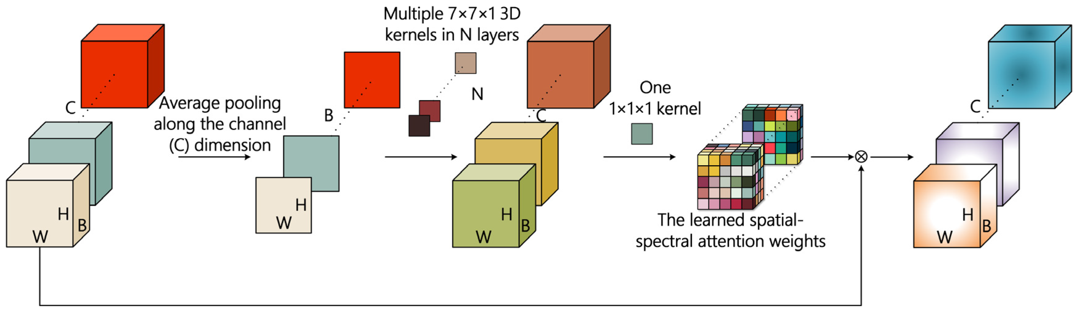
3.3. Light-Weight Attention-Enhanced Spatial–Spectral Feature Learning

There are two drawbacks to 3D convolution. On the one hand, the commonly used convolution kernel size, such as $3\times 3\times 3$, has a limited field of perception. On the other hand, the four-dimensional tensor extracted by 3D convolution demands high computational resources. To further refine the features extracted by 3D convolution, the lightweight attention-enhanced 3D convolution (LA-3D-Conv) structure is proposed.

Let the hyperspectral image dimension be $H\times W\times B$, where $H$ and $W$ are spatial dimensions, and $B$ is the spectral dimension. First, a vanilla 3D convolution layer is adopted to primarily investigate the joint spatial–spectral features and build 4D spatial–spectral feature space, $F_{3D}$, with dimension $H\times W\times B\times C$. It should be noted that the 4D feature space is essential since the spectral dimension is preserved, which is the main difference between 3D convolution and 2D convolution. To achieve lightweight feature refinement, the average pooling is performed along the channel dimension, and the pooled feature dimension is $H\times W\times B\times 1$. The spatial features are refined using two convolutional layers with kernels size $7\times 7\times 1$, and spectral features are further integrated. Zero padding is adopted to keep the feature dimension constant, and ReLU is served as the activation function. The feature map dimension is adjusted to $H\times W\times B\times 1$ using one convolutional layer with kernel size $1\times 1\times 1$, and the sigmoid function is adopted to map the learned features to (0, 1) as weights. The final refined features will be obtained by broadcast multiplication between $F_{3D}$ and spatial–spectral feature weight. The above operation can be expressed by the following equation:

$$Attention\left(F_{3D}\right)=f_{111}\left(f_{771}{}^2\left(GA{P}_C\left(F_{3D}\right)\right)\right)$$

(5)

$$F_{refined}=F_{3D}⨂Attention\left(F_{3D}\right)$$

(6)

where $F_{refined}$ represents the final refined features; $⨂$ represents tensor multiplication with a broadcast mechanism. The complete LA-3D-Conv structure is shown in Figure 2. To make the network training smooth, a residual structure is adopted to fuse the original features and the features refined by LA-3D-Conv, which is shown in Figure 1. In addition, a batch normalization layer is added after the residual structure to improve the feature robustness.

Our proposed lightweight attention-enhanced 3D convolution will facilitate spatial–spectral feature learning in two aspects. First, the dimensionality of the 3D convolutional feature map is reduced from $H\times W\times B\times C$ to $H\times W\times B\times 1$ so that channel-wise redundancy has been filtered. Second, global spatial features are enhanced, and spectral features are further integrated during attention weight generation.

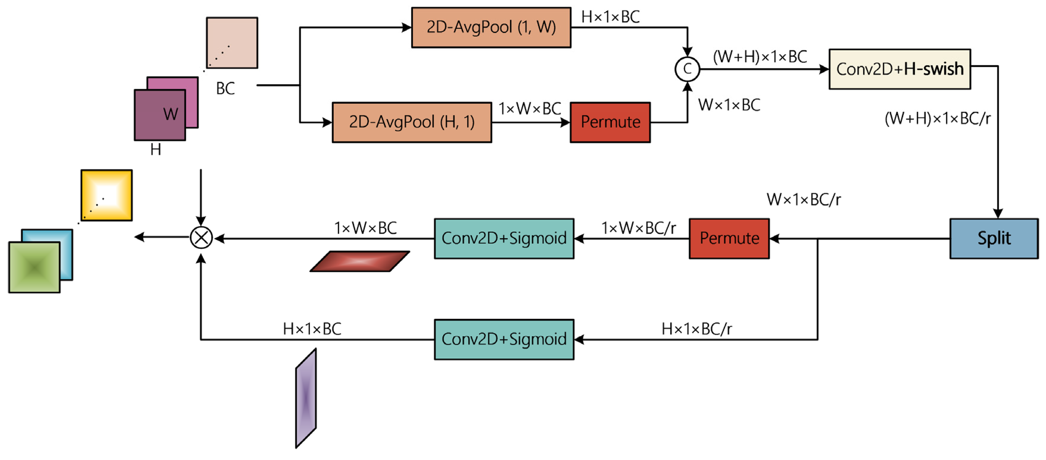
3.4. Spatial Feature Refinement Based on Coordinate Attention

The 4D spatial–spectral features extracted by 3D convolution in a mixed CNN model are reshaped into 3D tensors and contain feature groups with large differences, which cannot be effectively explored by vanilla 2D convolution. Aiming at the above problems, a spatial feature refinement unit based on coordinate attention (CA) is adopted. The original coordinate attention is proposed in the literature [54] and is aimed to enhance mobile network design by supplying direction-aware and position-sensitive attention maps. In this paper, we apply CA to obtain long-range dependencies across the restructured channel dimension and positional information, which are difficult to capture by 3D convolution with limited kernel size. It should be noted that BN is not adopted within CA in this paper. The coordinate attention schematic is shown in Figure 3.

The 3D convolution extracts features of dimension $H\times W\times BC$ after reshaping. In order to introduce coordinate information, the feature map is pooled in both X-direction and Y-direction with two pooling kernels of $\left(1, W\right)$ and $\left(H, 1\right)$, respectively. The pooling layers yield features of dimensions $H\times 1\times BC$ and $1\times W\times BC$. To further learn the channel importance, the two sets of features are aligned and connected to obtain a fused feature of dimension $\left(W+H\right)\times 1\times \left(BC\right)$. The channel dimension is then reduced, and the position information is embedded. The process of feature concatenation and dimensionality reduction is shown in Equation (7):

$$f_{dr}=act(F_{1\times 1}([e^w,e^h]))$$

(7)

where $f_{dr}$ represents the dimension reduced features, and the channel dimension is reduced to $\left(BC\right)/k$; $F_{1\times 1}$ represents the $1\times 1$ convolution; $act()$ represents the non-linear activation function, and H-Swish is adopted according to the literature [55]. It should be noted that the feature interaction in different directions is achieved since each spatial feature map of dimension $\left(W+H\right)\times 1$ shares convolution weights. Before the channel dimension is recovered, $f_{dr}$ is separated into $f^w$ and $f^h$ along the spatial dimension, with dimensions $W\times 1\times \left(BC\right)/r$ and $H\times 1\times \left(BC\right)/r$, respectively. The dimension of $f^w$ is adjusted to $1\times W\times \left(BC\right)/r$, keeping the same order as the initial pooling dimension. The $f^w$ and $f^h$ were then restored to their initial dimensions using two $1\times 1$ convolution layers, and the feature values were mapped to (0, 1) using the sigmoid activation function as the attention weights. The above calculation process is shown in the following equation:

$$g^w=s\left(F_w\left(f^w\right)\right)$$

(8)

$$g^h=s\left(F_h\left(f^h\right)\right)$$

(9)

where $g^w$ and $g^h$ are the X- and Y-direction attention weights with dimensions $1\times W\times \left(BC\right)$ and $H\times 1\times \left(BC\right)$, respectively; $s()$ is the sigmoid function. The refined spatial–spectral features are obtained by tensor multiplication of $g^w$, $g^h$, and the input features.

Through coordinate attention, the global dependencies of spectral-channel features can be fully explored, and the position-sensitive information is embedded, which facilitates the network to find the spatial locations and valuable band intervals that are important for HSIC.

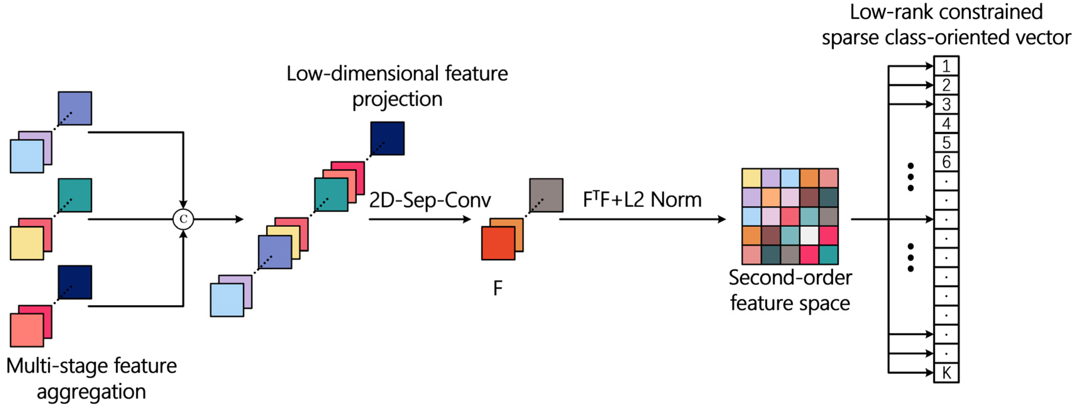
3.5. Low-Rank Constrained Second-Order Pooling for Final Classification

Compared to the commonly used fully connected (FC) layer or global pooling, second-order pooling can provide global image representation by computing the inner product of all given feature pairs. As for diverse spatial–spectral feature groups extracted by LA-3D-Conv and coordinate attention, all pairwise interactions among the multi-stage features can be considered. However, this second-order manner produces a high-dimension feature vector, which brings large parameter numbers and increases computational resources. In fact, it is found that in a high-dimensional feature space built by CNN models, less than 5% of the total features are informative [56].

Inspired by the literature [57,58], this paper introduces a simple low-rank constraint on the spatial–spectral features. A compact low-dimension vector will be learned for each category based on the second-order features. The adopted low-rank constraint method can be seen as a simplification of the method in the literature [58], and the diagram is shown in Figure 4.

Suppose the dimension of the multi-stage spatial–spectral features, which is denoted as $F_{mul}$, is $S_h\times S_w\times M$. First, a depth separable convolutional layer is adopted for low-dimension feature projection. Depth separable convolution is divided into depth-wise convolution and point-wise convolution. Depth-wise convolution can learn the unique spatial features of each channel without any interaction between channels. Point-wise convolution acts as a learnable nonlinear position-wise feature embedding tool. Let the embedded feature dimension be $S_h\times S_w\times C$, which is represented by $F_{ss}$. By computing the inner product of each spatial location feature vector of $F_{ss}$, which is denoted as $x_i\in R^C\left(1\le i\le S_h\times S_w\right)$, and its transposed vector, the second-order feature representation, $F_{sop}$, with dimension $C\times C$ can be obtained. The above calculation process can be expressed succinctly in matrix form as follows:

$$F_{sop}=F_{ss}^T{F}_{ss}$$

(10)

To enhance the feature robustness, L2 normalization is adopted after the second-order feature calculation.

The commonly used parameterization of the multiclass output layer with softmax activation function is known as $Y=softmax\left(F_O{W}_O+b_O\right)$, where $F_O$ represents the extracted high-level features; $W_O$ and $b_O$ are the corresponding weight and bias of the output layer. Second-order pooling describes inter-channel correlation in detail and inevitably introduces redundant channels. Therefore, a low-rank constraint is introduced to learn a compact low-dimensional vector for each class. Let the parameters to be learned for each class based on second-order features be the weights $W$ and biases $b$, where $W\in R^{C\times C}$ and corresponds to the dimensions of $F_{sop}$. Suppose $W^{*}$ is the optimal parameter matrix. The literature [57] has proved that $W^{*}$ is a symmetric matrix, and the eigen-decomposition of $W^{*}$ can be expressed in the following formula:

$$W^{*}=\Psi \Sigma {\Psi }^T={\Psi }_{+}{\Sigma }_{+}{\Psi }_{+}^T-{\Psi }_{-}\left|{\Sigma }_{-}\right|{\Psi }_{-}^T$$

(11)

where ${\Sigma }_{+}$ and ${\Sigma }_{-}$ are diagonal matrices containing positive and negative eigenvalues, respectively; ${\Psi }_{+}$ and ${\Psi }_{-}$ are the corresponding eigenvectors. Denote $U_{+}={\Psi }_{+}{\Sigma }_{+}^{\frac{1}{2}}$ and $U_{-}={\Psi }_{-}{\left|{\Sigma }_{-}\right|}^{\frac{1}{2}}$, and then the above decomposition can be written as follows:

$$W^{*}=U_{+}{U}_{+}^T-U_{-}{U}_{-}^T$$

(12)

Equation (12) indicates that $W^{*}$ may have a low-rank decomposition. Suppose the matrix rank of $W^{*}$ is $r$ and satisfies $rank\left(W\right)=r\ll C$, i.e., $U_{+}\in R^{C\times r/2}$, $U_{-}\in R^{C\times r/2}$, then $W^{*}$ can be approximated by two low-rank matrices. In this case, only $U_{+}$ and $U_{-}$ need to be parameterized and serve as the weights in the output layer, not the original weight matrix $W$.

HSIC tasks are fine-grained classification problems, thus $N$ classes need to learn $N$ sets of weights $W$ and biases $b$. The low-rank weight parameter matrix of the $i$th class can be obtained from Equation (12) as $W_i=u_{+}{}_i{u}_{+}{}_i^T-u_{-}{}_i{u}_{-}{}_i^T$, where $W_i\in R^{C\times C}$. The probability value of each class can be calculated by the following formula:

$$P=softmax\left(\mathrm{vec}\left(F_{sop}\right)\mathrm{vec}\left(W\right)+b\right)$$

(13)

where $P=\left[p_1,p_2,\dots ,p_N\right]$ is the probability of each category; $W$ = $\left[W_1,W_2,\dots ,W_N\right]$ is the sparse low-rank weight parameter matrix list computed through $W_i=u_{+}{}_i{u}_{+}{}_i^T-u_{-}{}_i{u}_{-}{}_i^T$; $b=\left[b_1,b_2,\dots ,b_N\right]$; $vec()$ represents vectorization operations. The classification result is obtained by Equation (13), and the parameter number will be $CrN$. Since $r\ll C$, the parameter number and the computation burden can be remarkably reduced. Considering the balance of model size and classification accuracy, $r$ is set to 16 in the proposed LAMFN.

4. Experimental Results and Analysis

4.1. Experimental Datasets

To verify the effectiveness and generalization of the proposed method for different types of HSI datasets, four challenging hyperspectral datasets with various spatial and spectral resolutions were used for classification experiments. The experimental datasets include classical and widely adopted Indian Pines (IP), Pavia Center (PC), Houston (HU), and the latest released WHU-HongHu (WHU) dataset with high spatial resolution. The detailed information of the experimental datasets is shown in

Table 2. Detailed information of the experimental datasets.

	IP	PC	Houston	WHU
Spectral Range (μm)	0.4–2.5	0.43–0.86	0.38–1.05	0.4–1.0
Number of Bands	200	102	144	270
Data Size	145 × 145	1096 × 715	349 × 1905	940 × 475
Spatial Resolution (m)	20	1.3	2.5	0.043
Number of Classes	16	9	15	22
Number of Labeled Data	10,249	148,152	15,029	386,693
Number of Training Data	80	45	75	110

, and the brief introduction is as follows:

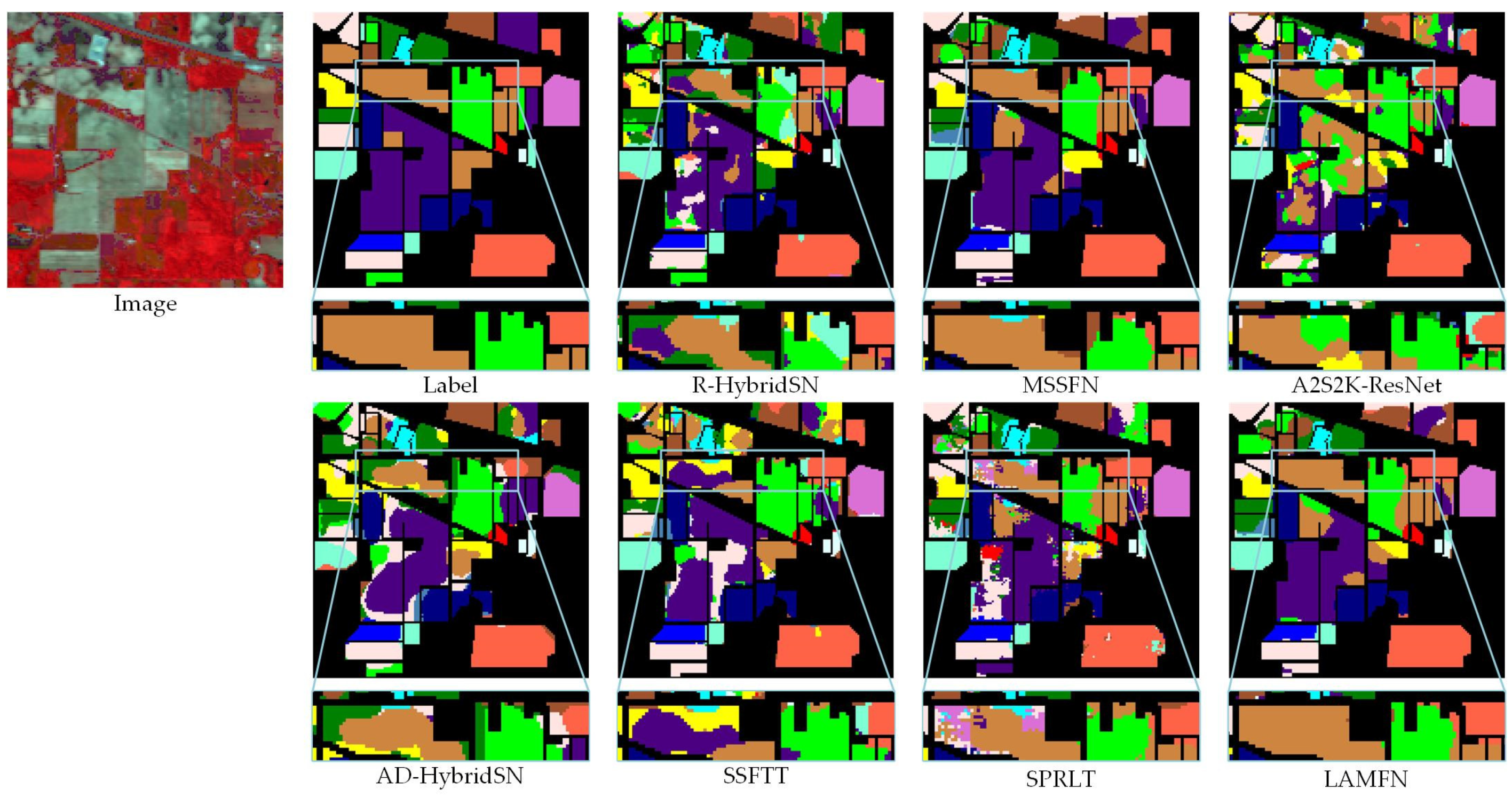
• IP is a classical dataset that is widely used to evaluate HSIC algorithms. Since its spatial resolution is low and many mixed pixels exist, the IP dataset can test the effectiveness of the algorithm in extracting robust features. The remaining three datasets have large image sizes and high spatial resolution.
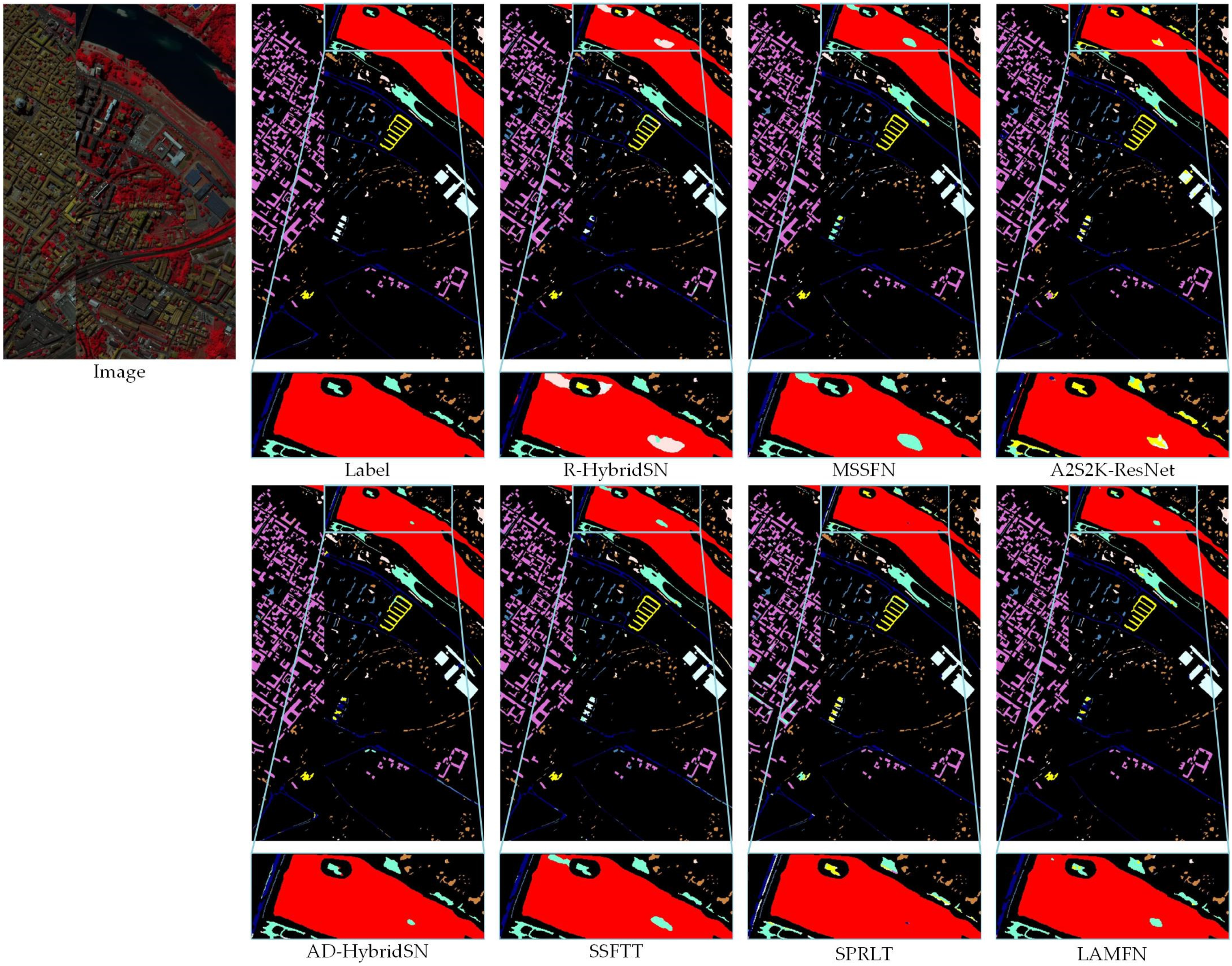
• PC has an original size of $1096\times 1096$. However, some areas have no information and they have been discarded. The processed PC dataset still has a large image size, which is $1096\times 715$. This scene contains many objects with similar textures and colors that often appear in urban areas.
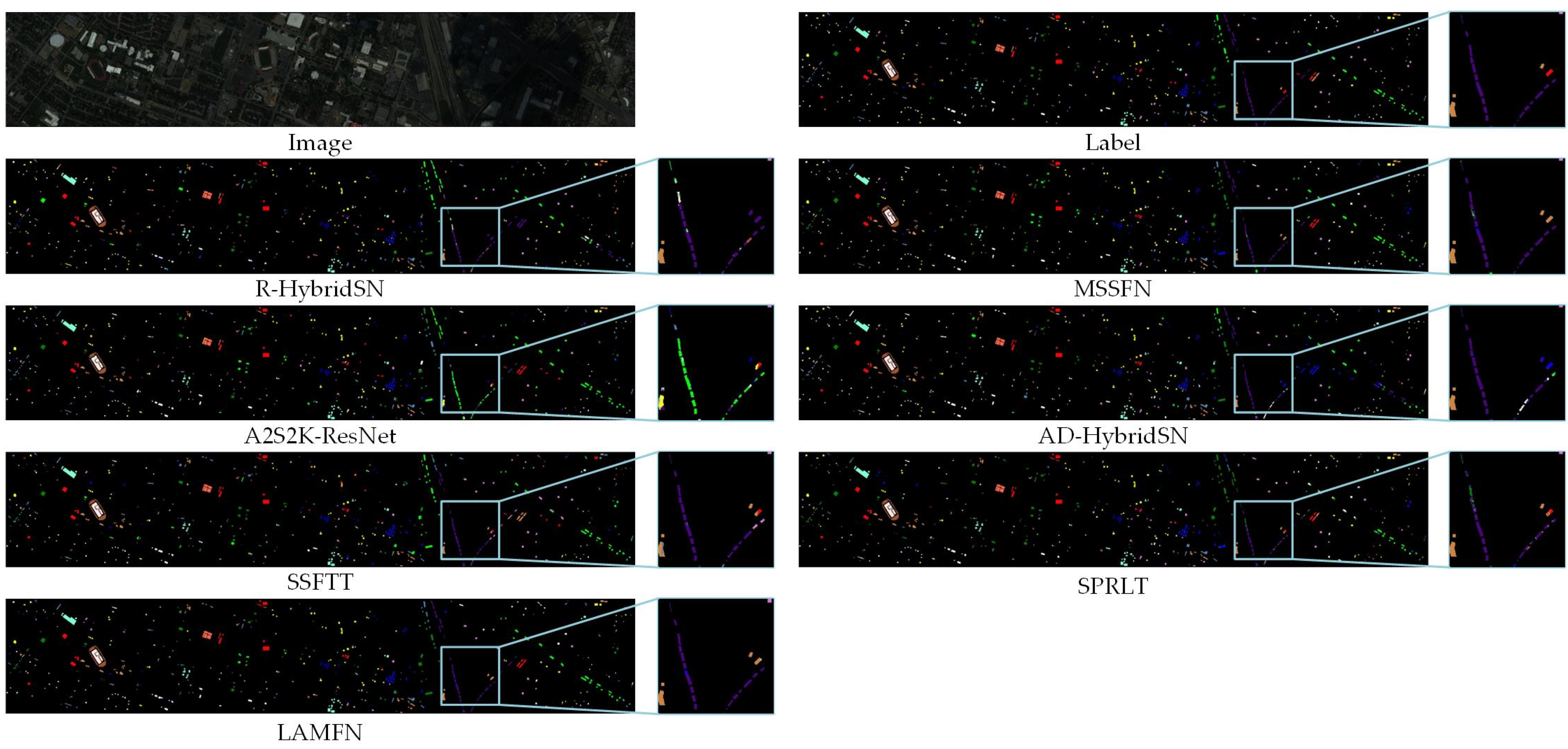
• The HU dataset was originally released during the 2013 Data Fusion Contest by the Image Analysis and Data Fusion Technical Committee of the IEEE Geoscience and Remote Sensing Society, so it is also named “2013_IEEE_GRSS_DF_Contest”. This dataset is challenging due to its large image size and sparse distribution of available samples.
• The WHU dataset is a recently released hyperspectral dataset collected by unmanned aerial vehicles (UAVs) with extremely high spatial resolution [59]. The ground objects include 22 plant species with similar colors and textures, which greatly challenges the classification algorithm.

To sum up, the experimental datasets are mainly hyperspectral datasets with high spatial resolution. The ground objects include artificial objects in urban areas and various crops and plants in rural areas. In the following experiments, only five samples of each class were randomly selected for model training. The generalization of the proposed model for small sample HSIC tasks will be fully validated in different hyperspectral scenes.

4.2. Contrast Models

In order to assess the effectiveness of the proposed model, several advanced deep learning models published in recent years were used as contrast models, including R-HybridSN [25], MSSFN [41], A2S2K-ResNet [60], AD-HybridSN [30], SSFTT [36], and SPRLT [37]. The above contrast models can be broadly classified into three categories and will be briefly described as follows:

• R-HybridSN and MSSFN are both residual CNN models, which are focused on small sample HSIC tasks. R-HybridSN adopts residual learning and depth separable convolution to refine the feature learning process. MSSFN further improves the classification accuracy using cascaded feature fusion patterns and second-order pooling.
• A2S2K-ResNet and AD-HybridSN are two convolution-attention fusion models. AD-HybridSN is a mixed CNN model. Attention modules are inserted after each convolutional layer to achieve spatial–spectral feature refinement. A2S2K-ResNet adopted selective kernel attention in the first layer and efficient channel feature attention in the successive layers.
• SSFTT and SPRLT are two very recently proposed transformer-based HSIC models. SPRLT adopts a spatial partition restore (SPR) module that is designed to split the input patch into several overlapping continuous sub-patches as sequential. SSFTT use 3D convolution and 2D convolution to build prior spatial–spectral feature space for subsequent transformer block. Both of them improve the applicability of transformer block in HSIC tasks by designing a novel feature organization approach.

4.3. Experimental Setup

The experimental hardware environment is computer equipped with an Intel i9-11900K CPU, an RTX 3090 GPU, and the RAM is 128G. The main experimental environment is Python 3.7, Tensorflow 2.8, and Pytorch 1.8. The model in this paper is based on Keras, which is a high-level deep learning framework running on top of Tensorflow.

LAMFN adopts Adam as the optimizer. The learning rate is set to 0.001, and the number of training epochs is set to 100. It should be noted that we found that LAMFN can obtain better results in the four datasets by monitoring training loss instead of training accuracy. In addition, almost the same experimental results can be obtained by directly testing the model obtained in the last epoch.

As for the contrast models, the patch size, dimension reduction setting, number of bands, optimizer, and learning rate are set according to the original papers. The training and testing process of SSFTT, SPRLT, and A2S2K-ResNet is completed on Pytorch deep learning framework. In our experiments, we used some open-source codes to process experimental data, train and test the contrast models, and the codes can be found at https://github.com/zgr6010/HSI_SSFTT and https://github.com/ZhaohuiXue/SPRLT-Net (accessed on 1 October 2022).

To ensure that the models can be well trained, the training epochs of A2S2K-ResNet and SPRLT are set to 200, and the training epochs of other contrast models are set to 100. The experimental datasets were randomly divided into a training set and a testing set using the same random seed in all experiments to guarantee a fair comparison. To be specific, we use Numpy library to divide training and testing samples randomly, and the seed number was set to 0. In all the experiments, five samples of each class are selected to train the model.

4.4. Comparison with the Contrast Models

In order to verify the effectiveness of the proposed method, classification experiments are performed using the IP, PC, HU, and WHU datasets. The contrast methods cover the advanced models proposed in recent years. The experiments were run continuously ten times, and the average values were taken as the experimental result. The accuracy of each class, OA, AA, and kappa, which are commonly used in hyperspectral classification, are used to measure the classification performance. The standard deviation of the last three statistics was given after ± to measure the accuracy fluctuation degree.

Table 3. Classification results (%) of different models in IP dataset.

No.	Residual CNN		Attention-Based CNN		Transformer Models		Proposed
	R- HybridSN	MSSFN	A2S2K- ResNet	AD- HybridSN	SSFTT	SPRLT	LAMFN
1	96.10	99.76	96.34	98.05	98.29	96.83	98.78
2	50.39	69.28	40.77	54.34	49.09	59.72	64.40
3	48.62	67.14	48.17	69.02	56.28	60.40	66.02
4	80.43	93.45	81.42	82.24	90.39	93.06	90.95
5	75.25	82.43	69.27	76.46	75.67	81.80	83.37
6	92.87	96.47	88.84	94.44	92.76	95.90	96.72
7	100.00	100.00	99.13	100.00	100.00	100.00	99.57
8	96.00	98.20	86.17	95.52	95.50	92.09	99.70
9	100.00	99.33	99.33	100.00	100.00	98.67	100.00
10	63.42	69.60	56.85	55.18	72.03	68.79	74.01
11	55.03	63.98	45.03	47.78	57.29	54.36	67.36
12	53.74	67.11	52.13	47.79	49.88	66.89	80.43
13	99.65	99.55	97.90	99.25	98.50	99.35	98.55
14	81.13	95.02	84.69	84.65	84.38	89.32	93.01
15	76.30	92.41	79.97	79.48	82.26	92.34	86.90
16	98.64	98.86	96.93	96.82	90.91	99.32	98.30
Kappa	62.32 ± 2.53	74.58 ± 3.21	57.05 ± 6.73	62.62 ± 2.85	64.86 ± 3.64	68.70 ± 2.49	75.41 ± 3.44
OA	66.34 ± 2.42	77.33 ± 2.89	61.35 ± 6.28	66.40 ± 2.79	68.68 ± 3.46	71.95 ± 2.37	78.15 ± 3.14
AA	79.22 ± 1.44	87.04 ± 1.59	76.43 ± 5.32	80.06 ± 1.92	80.83 ± 1.93	84.30 ± 1.13	87.38 ± 1.55

,

Table 4. Classification results of different models in PC dataset.

No.	Residual CNN		Attention-Based CNN		Transformer Models		Proposed
	R- HybridSN	MSSFN	A2S2K- ResNet	AD- HybridSN	SSFTT	SPRLT	LAMFN
1	98.00	99.40	99.14	99.52	98.37	99.16	99.60
2	79.98	84.07	84.66	84.61	81.79	84.58	84.73
3	87.49	81.90	96.05	87.06	88.28	83.06	88.96
4	86.09	98.61	93.13	97.93	95.81	72.31	95.24
5	80.53	82.87	88.70	84.80	88.93	85.93	90.47
6	86.43	91.71	96.06	93.88	83.48	87.62	98.41
7	90.03	91.08	83.36	91.08	91.09	87.93	89.72
8	94.52	98.38	96.77	96.79	98.64	95.71	98.78
9	77.07	86.12	98.03	88.44	92.01	91.89	91.59
Kappa	90.69 ± 2.55	94.44 ± 1.82	94.49 ± 1.71	94.42 ± 1.28	93.68 ± 1.64	92.40 ± 2.78	96.01 ± 0.84
OA	93.34 ± 1.91	96.06 ± 1.30	96.09 ± 1.23	96.04 ± 0.92	95.51 ± 1.17	94.59 ± 2.03	97.18 ± 0.60
AA	86.68 ± 1.07	90.46 ± 2.85	92.88 ± 1.47	91.57 ± 1.45	90.93 ± 2.12	87.58 ± 3.64	93.05 ± 1.12

,

Table 5. Classification results of different models in HU dataset.

No.	Residual CNN		Attention-Based CNN		Transformer Models		Proposed
	R- HybridSN	MSSFN	A2S2K- ResNet	AD- HybridSN	SSFTT	SPRLT	LAMFN
1	72.05	84.91	82.10	77.44	76.37	86.93	86.89
2	78.49	84.45	78.59	81.68	81.00	80.32	83.96
3	91.45	98.03	88.15	97.12	98.24	99.54	98.37
4	79.48	88.35	90.66	81.44	81.32	86.19	90.40
5	89.30	92.78	79.89	96.98	98.01	99.69	98.48
6	88.38	85.09	77.03	88.38	88.22	93.47	86.97
7	41.76	70.89	62.91	67.17	66.80	56.35	71.10
8	52.46	52.97	45.81	49.50	42.99	58.07	54.87
9	47.89	69.03	59.37	61.11	50.22	37.67	67.64
10	58.36	76.38	41.87	63.53	62.12	62.52	73.40
11	57.83	73.72	47.46	70.67	74.19	64.67	84.37
12	68.45	74.90	45.82	71.95	65.13	57.56	73.08
13	87.78	82.50	90.91	94.70	90.60	67.89	92.72
14	100.00	100.00	97.07	99.93	99.76	100.00	100.00
15	99.05	96.41	92.41	99.88	98.09	99.53	96.05
Kappa	67.18 ± 1.90	78.04 ± 2.19	65.47 ± 3.94	74.50 ± 2.95	72.20 ± 2.46	70.97 ± 2.09	79.84 ± 2.82
OA	69.56 ± 1.77	79.68 ± 2.03	68.01 ± 3.63	76.35 ± 2.75	74.26 ± 2.29	73.11 ± 1.95	81.35 ± 2.61
AA	74.18 ± 1.49	82.03 ± 1.69	72.00 ± 3.77	80.10 ± 2.31	78.20 ± 1.90	76.69 ± 1.71	83.89 ± 2.17

and

Table 6. Classification results of different models in WHU dataset.

No.	Residual CNN		Attention-Based CNN		Transformer Models		Proposed
	R- HybridSN	MSSFN	A2S2K- ResNet	AD- HybridSN	SSFTT	SPRLT	LAMFN
1	83.77	75.44	73.07	80.63	82.23	81.02	85.62
2	57.62	75.88	68.98	80.79	71.03	67.99	73.99
3	75.19	81.19	81.64	75.22	83.52	77.88	83.27
4	86.41	94.92	69.54	91.49	84.56	79.06	95.71
5	60.50	93.54	68.35	86.23	78.71	74.74	92.79
6	90.24	93.03	86.38	89.97	89.12	78.05	93.61
7	51.49	66.98	40.20	63.94	46.70	42.38	68.29
8	60.11	62.97	37.14	66.06	58.84	28.80	56.19
9	93.01	92.89	90.29	92.75	90.60	92.36	94.21
10	42.60	83.75	65.16	66.84	47.48	52.29	80.02
11	57.00	73.57	46.42	59.18	43.88	26.08	74.74
12	44.28	74.67	60.33	52.24	49.06	52.68	73.47
13	43.62	57.55	52.50	52.48	49.24	44.83	62.05
14	77.41	83.49	71.25	88.72	65.27	60.21	86.35
15	96.04	99.71	91.35	95.88	98.77	86.61	98.01
16	84.32	95.58	82.85	86.34	89.98	76.09	95.13
17	86.42	90.99	77.52	77.88	83.36	69.19	89.62
18	91.74	97.83	87.08	95.80	89.78	58.14	95.87
19	82.70	92.61	78.80	87.64	73.48	47.68	85.53
20	80.82	95.99	77.49	88.50	59.88	79.99	93.66
21	75.28	97.43	78.16	89.52	83.08	67.69	97.30
22	76.49	94.62	86.33	86.78	85.59	87.03	94.14
Kappa	71.88 ± 2.62	83.84 ± 2.12	64.27 ± 4.13	78.47 ± 2.69	71.16 ± 3.98	64.05 ± 5.56	84.90 ± 1.82
OA	77.06 ± 2.23	87.04 ± 1.79	69.71 ± 3.98	82.61 ± 2.26	76.38 ± 3.68	70.07 ± 5.17	87.93 ± 1.49
AA	72.59 ± 2.28	85.21 ± 1.29	71.40 ± 2.74	79.77 ± 2.71	72.92 ± 1.44	65.03 ± 3.59	84.98 ± 1.31

show the experimental results of IP, PC, HU, and WHU datasets, respectively.

By analyzing the quantitative experimental results from Table 3, Table 4, Table 5 and Table 6, the following findings can be drawn:

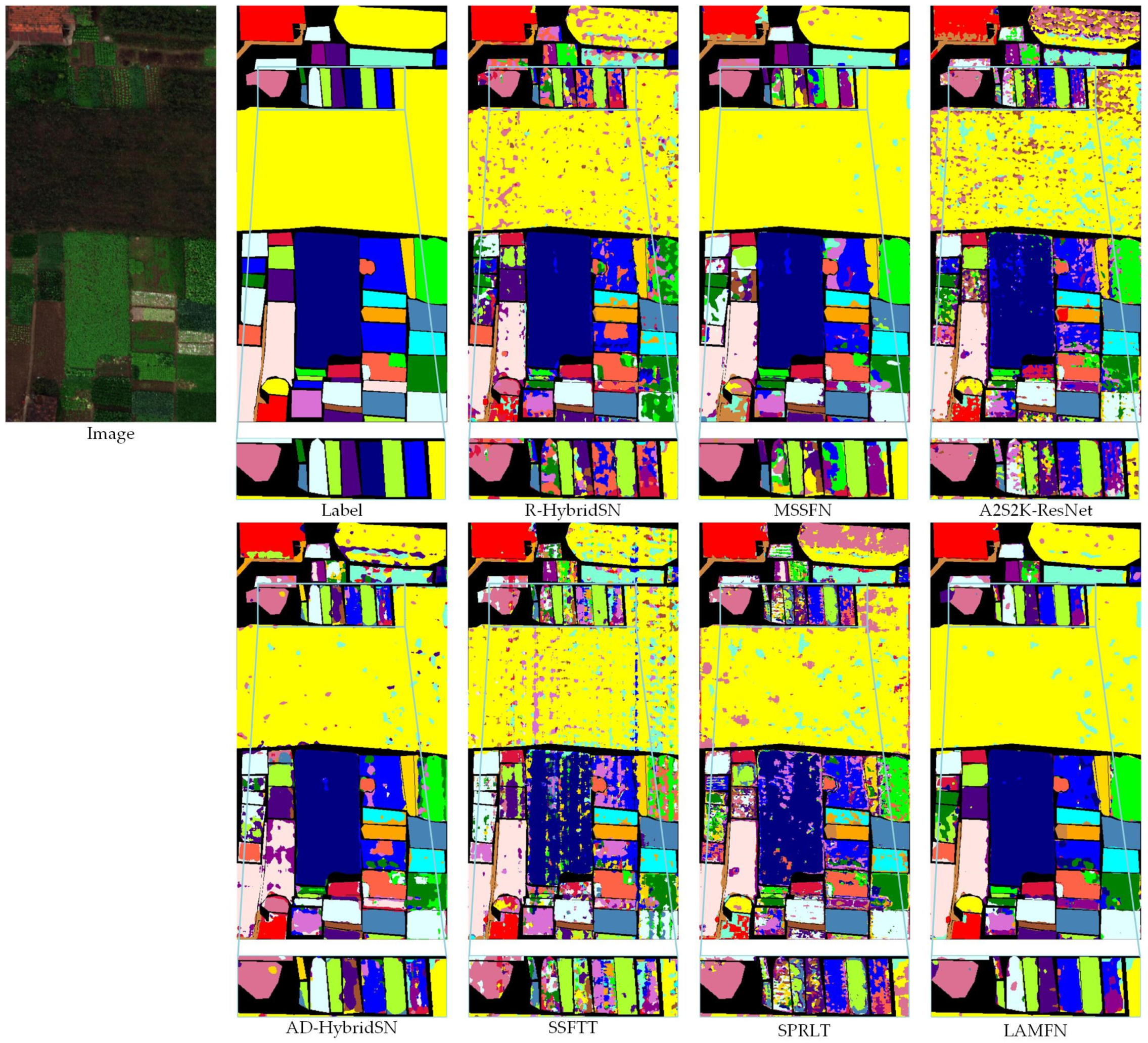
• Various methods show distinct generalization properties for different datasets. For example, the experimental results of R-HybridSN and SPRLT with larger model sizes are not ideal for the four datasets, which indicates the over-fitting phenomenon is prominent. On the contrary, MSSFN and SSFTT performed relatively better. It is believed that the parameter number is the superficial reason, while the real reason is the difference in feature extraction ability and parameter redundancy caused by the model structure.
• Two transformer-based models, SSFTT and SPRLT, can achieve comparable results with other models in PC and WHU, but the results in IP and HU are not ideal. Since patch-based structures are adopted, the global feature learning ability of the self-attention module is limited to a large extent. Therefore, the VIT-based approaches may consider continued improvements in data organization.
• Quantitative experimental results demonstrate the effectiveness of LAMFN. In the four datasets, the proposed method achieved the highest OA and kappa. Compared with the second-best model, MSSFN, the OA of LAMFN has improved by 0.82%, 1.12%, 1.67%, and 0.89% in IP, PC, HU, and WHU datasets, respectively. The AA value of LAMFN was slightly lower than MSSFN in the WHU dataset.
• Although the LAMFN achieved the best OA value in four datasets, it achieved the lowest standard deviation in only two datasets, namely PC and WHU. The stability of the LAMFN for some datasets needs to be further improved.

Figure 5, Figure 6, Figure 7 and Figure 8 show the predicted maps for all models, which can be seen as a visual reference to model performance assessment. The areas obtained by LAMFN with less noise have been highlighted to show the effectiveness of our proposed model. Overall, the proposed LAMFN has fewer misclassifications and omissions and generalizes well to different datasets with only five samples per class.

4.5. Running Time Analysis

In this paper, the algorithm complexity has been paid considerable concern at the beginning of the model design.

Table 7. Running related parameters of the LAMFN and the contrast models.

Model	R- HybridSN	MSSFN	A2S2K- ResNet	AD- HybridSN	SSFTT	SPRLT	LAMFN
Input size	15 × 15 × 16	15 × 15 × 16	9 × 9 × 200	15 × 15 × 16	13 × 13 × 30	9 × 9 × 200	15 × 15 × 16
Parameter	719,112	159,012	373,184	366,662	148,488	839,728	157,826
Training Time (s)	16.6	24.8	341.4	20.0	3.0	239.3	29.1
Testing Time (s)	49.2	60.7	116.0	76.5	16.9	184.0	103.9

lists the input data size, parameter number (takes IP dataset as an example), training time, and testing time of LAMFN and all the contrast models. The WHU dataset with the largest data size is selected for running time display.

The model in this paper has good lightweight characteristics. First, the proposed model is comparable to MSSFN and SSFTT in terms of parameter number, while its accuracy exceeds those two models. This phenomenon indicates that our model can learn more robust HSI features with lower parameter redundancy. In terms of running time, the shorter running time indicates that fewer computational resources are required. The running time of A2S2K-ResNet is significantly longer than the other models since many 3D convolutional layers arranged in complex structures are used to extract features directly from hyperspectral images. The proposed model has moderate running time compared to the contrast models.

5. Discussion

5.1. Model Design Analysis of LAMFN

The overall effectiveness of the proposed method is verified in Section 4.4: Comparison with the Contrast Models. In order to further evaluate the detailed designs in LAMFN for small sample HSIC tasks, ablation experiments were conducted to test the improvement of FA, LA-3D-Conv, CA, and low-rank SOP on each dataset.

For FA, PCA was used for contrast experiments, and the other settings remained the same. For SSF, two-layer 3D convolution with residual structure was used to build a contrast model. The number of convolution kernels is consistent with the method in this paper, and the size of convolution kernels is set as $3\times 3\times 3$. For CA, blank control was performed, which means CA will be removed from LAMFN. For LRSOP, global average pooling (GAP) and original second-order pooling (SOP) will be used for comparison. Other experimental settings are consistent with the experiments in Section 4.4: Comparison with the Contrast Models, and the OA results are shown in

Table 8. OA results (%) of ablation model experiments.

Model	Description	IP	PC	Houston	WHU
LAMFN	proposed	78.15	97.18	81.35	87.93
C1	Replacing FA with PCA	74.74	97.27	81.14	84.36
C2	Replacing LA-3D-Conv with residual $3\times 3\times 3$ 3D-Conv	77.07	96.98	80.23	87.02
C3	Without CA	77.06	97.05	80.94	86.96
C4	Replacing LRSOP with GAP	77.39	95.66	79.01	87.67
C5	Replacing LRSOP with SOP	77.35	96.99	80.87	86.56

.

The effectiveness of FA has been verified through the comparison between the results of LAMFN and C1. In order to further explore the influence of the number of bands on PCA and FA, a more detailed comparative experiment was conducted, with the number of bands ranging from 12 to 28. The experimental results are shown in

Table 9. OA results (%) of different band number using FA and PCA.

Band	IP		PC		Houston		WHU
	FA	PCA	FA	PCA	FA	PCA	FA	PCA
12	77.70	72.62	97.18	97.27	81.18	80.31	87.27	84.08
16	78.15	74.74	97.18	97.27	81.35	81.14	87.93	84.36
20	77.63	71.87	96.86	97.24	81.77	80.89	86.80	83.80
24	78.07	73.00	97.07	96.83	80.59	81.16	87.06	84.16
28	77.41	72.47	96.94	96.56	80.49	79.87	86.73	86.14

. In addition, there is a big difference between FA and PCA in terms of dimensionality reduction time. Taking the WHU dataset as an example,

Table 10. Running time (second) of PCA and FA with different number of bands in WHU dataset.

	12	16	20	24	28
PCA	3.0	3.0	3.7	5.0	4.0
FA	34.8	31.0	49.0	64.8	63.9

shows the running time of PCA and FA with different number of bands.

By analyzing the experimental results in Table 9 and Table 10, three conclusions can be drawn as follows:

• When the number of bands is 16, FA achieves the overall best accuracy (measured in average) in the four datasets. By increasing the number of bands, only the accuracy in the IP data set continues to improve, while the accuracy of the other datasets tends to decrease. Compared with PCA, the FA dimension reduction method achieves the optimal factor number earlier.
• FA significantly outperforms the PCA method when the number of bands is 16. In both IP and WHU datasets, FA has an absolute advantage. However, FA achieves slightly lower accuracy in the PC dataset than using PCA. As the number of bands increases, the accuracy obtained by PCA improves significantly in IP and to a lesser extent in other datasets. Overall, there is a large gap between PCA and FA methods.
• PCA significantly outperforms FA in terms of resolving time. When the band number is 16, the resolving time of FA is 28.0 s slower than that of PCA. When the number of bands is taken as 24, the gap increases to 59.8 s. The slowdown is due to the fact that the FA takes into account the covariance of all input pixels. The extended solution time when the number of bands is taken as 16 is acceptable, given the resulting accuracy improvement.

Through the above analysis, the effectiveness and applicability of FA in hyperspectral small sample classification is further validated. On the one hand, the data covariance can effectively utilize the sample information and improve classification accuracy. On the other hand, for the trade-offs of resolving time, classification accuracy, and memory occupation, FA is sufficient to keep a small number of factors in the classification task.

The results in Table 8 completely verified all the refined designs for small sample HSIC tasks. The comparison between LAMFN, C2, and C3 demonstrates the improvements of lightweight SPS and CA modules. The comparison between LAMFN, C4, and C5 verified the improvement of low-rank second-order pooling compared to first-order pooling and direct second-order pooling. It should be noted that the LRSOP and SOP share one limitation compared to the GAP. When adopted for feature extraction, the dimension of the feature vector extracted by GAP will be much smaller than that of SOP or LRSOP since the explicit second-order feature calculation would square the channel number. Therefore, when being used for unsupervised feature extraction, such as in contrastive learning tasks, the number of channels needs to be further reduced. And this can be flexibly achieved by changing the kernel number of the 2D-Sep-Conv layer.

The motivation of LAMFN is to minimize the repetition of various features and reduce network redundancy. Multi-feature fusion is a widely adopted network design principle, but one of the key points may be ignored, namely, feature redundancy caused by the repetition of feature types. The concise feature extraction module with considerable variance is of great help to improve the classification accuracy. Based on this idea, LA-3D-Conv is designed to extract spatial–spectral features in a lightweight attention-based manner. CA is used to supplement positional information and cross-channel features ignored by 3D convolution. Then, different types of features are aggregated in a composite residual structure. In terms of feature utilization, LRSOP introduces low-rank constraints to reduce the number of parameters in the output layer while maintaining the selectivity advantage of the second-order features on different feature channels.

5.2. Comparison with Advanced Semi-Supervised Methods

In order to further verify and position the superiority of the proposed method, we compared LAMFN with some advanced semi-supervised methods proposed in recent years. Methods used for comparison include DFSL [46], DMVL [45], UM2L [48], and SC-EADNet [44]. The above methods include unsupervised feature learning and supervised fine-tunning, and they are briefly described below.

• The DFSL is a cross-domain meta-learning method. Firstly, the model is pre-trained in the source domain dataset to obtain the metric space. Then, the well-trained model extracts robust features, and the final classification can be achieved by a simple linear classifier using very few samples.
• The DMVL is a contrastive learning method. The two successive spectral vectors within each pixel are used for generating positive and negative samples for contrastive pretraining.
• The UM2L is an end-to-end cross-domain meta-learning method. The pretraining phase was performed in an unsupervised manner with multi-view constrained contrast learning.
• SC-EADNet combines contrastive learning with well-designed multiscale residual depth-separable convolutional networks.

The comparison results are shown in Table 9 (blank indicates that the dataset is not included in the above papers). For all the models, five samples from each class were selected to supervise the model training or fine-tuning process to ensure a fair comparison.

The comparison results in

Table 11. Comparison results with several advanced semi-supervised methods.

Model	IP	PC	Houston
LAMFN	78.15	97.18	81.35
DFSL	63.11	94.90	69.29
DMVL	78.01		78.55
UM2L	72.09	94.27
SC-EADNet	82.69		80.89

show that, as a supervised learning method, the classification performance of LAMFN has exceeded several advanced semi-supervised algorithms, such as DFSL, DMVL, and UM2L. Since simple residual backbones, such as ResNet-50 and its variants, are used to conduct semi-supervised learning in the above three frameworks, the good performance of LAMFN should be attributed to the superiority of the proposed model structure. The OA of SC-EADNet is better than our method in the IP dataset and lower in the HU dataset, which also shows that the well-designed network can better learn spatial–spectral features in unsupervised manners. However, which kind of combination of model structure and semi-supervised strategy contributes more to semi-supervised hyperspectral classification has no prior knowledge and needs further study.

6. Conclusions

To boost the classification performance for small sample HSIC tasks, the LAMFN classification framework was derived from dimension reduction, spatial–spectral feature extraction, and convolution feature post-processing. The effective fusion of multi-type features with sufficient variance and low redundancy is the core idea of the proposed LAMFN. Firstly, FA is used to reduce the dimensionality of hyperspectral data, and the spectral features are pre-learned from the perspective of data covariance. The attention-enhanced feature learning unit, LA-3D-Conv, is used to further refine the hyperspectral features. The LA-3D-Conv can effectively map the dimensionally reduced hyperspectral data to the four-dimensional feature space and highlight the valuable spatial–spectral feature intervals for classification in a lightweight manner. Then, coordinate attention is used to extract direction-sensitive and channel-aware information from the reshaped 3D features. A composite residual structure is used to aggregate the features learned by different stages. Finally, the classification is realized by using second-order pooling with low-rank constraints to learn compact class vectors for each class.

Extensive classification and module ablation experiments are carried out using four hyperspectral datasets with large differences, namely, IP, PC, HU, and WHU. In the experiments, the proposed method achieves the highest classification accuracy, and the running time is moderate, which verifies the effectiveness of the proposed method. In addition, we will try to combine the method in this paper with the idea of contrastive learning to enhance the method’s applicability in more scenarios. Due to the highly modular network design principle, we hope our model can promote the small sample hyperspectral classification research and also benefit other types of remote sensing image processing tasks.

References

1. Bouguettaya, A.; Zarzour, H.; Kechida, A.; Taberkit, A.M. Deep learning techniques to classify agricultural crops through UAV imagery: A review. Neural Comput. Appl. 2022, 34, 9511–9536. [Google Scholar] [CrossRef] [PubMed]
2. Wambugu, N.; Chen, Y.; Xiao, Z.; Tan, K.; Wei, M.; Liu, X.; Li, J. Hyperspectral image classification on insufficient-sample and feature learning using deep neural networks: A review. Int. J. Appl. Earth Obs. Geoinf. 2021, 105, 102603. [Google Scholar] [CrossRef]
3. Vali, A.; Comai, S.; Matteucci, M. Deep Learning for Land Use and Land Cover Classification Based on Hyperspectral and Multispectral Earth Observation Data: A Review. Remote Sens. 2020, 12, 2495. [Google Scholar] [CrossRef]
4. Rasti, B.; Hong, D.; Hang, R.; Ghamisi, P.; Kang, X.; Chanussot, J.; Benediktsson, J.A. Feature Extraction for Hyperspectral Imagery: The Evolution from Shallow to Deep: Overview and Toolbox. IEEE Geosci. Remote Sens. Mag. 2020, 8, 60–88. [Google Scholar] [CrossRef]
5. Ghamisi, P.; Maggiori, E.; Li, S.; Souza, R.; Tarablaka, Y.; Moser, G.; Giorgi, A.D.; Fang, L.; Chen, Y.; Chi, M.; et al. New Frontiers in Spectral–Spatial Hyperspectral Image Classification: The Latest Advances Based on Mathematical Morphology, Markov Random Fields, Segmentation, Sparse Representation, and Deep Learning. IEEE Geosci. Remote Sens. Mag. 2018, 6, 10–43. [Google Scholar] [CrossRef]
6. Li, X.; Liu, B.; Zhang, K.; Chen, H.; Cao, W.; Liu, W.; Tao, D. Multi-view learning for hyperspectral image classification: An overview. Neurocomputing 2022, 500, 499–517. [Google Scholar] [CrossRef]
7. Jia, S.; Jiang, S.; Lin, Z.; Li, N.; Xu, M.; Yu, S. A survey: Deep learning for hyperspectral image classification with few labeled samples. Neurocomputing 2021, 448, 179–204. [Google Scholar] [CrossRef]
8. Ahmad, M.; Shabbir, S.; Raza, R.A.; Mazzara, M.; Distefano, S.; Khan, A.M. Artifacts of different dimension reduction methods on hybrid CNN feature hierarchy for Hyperspectral Image Classification. Optik 2021, 246, 167757. [Google Scholar] [CrossRef]
9. Mohan, A.; Venkatesan, M. HybridCNN based hyperspectral image classification using multiscale spatiospectral features. Infrared Phys. Technol. 2020, 108, 103326. [Google Scholar] [CrossRef]
10. Luo, F.L.; Du, B.; Zhang, L.P.; Zhang, L.F.; Tao, D.C. Feature Learning Using Spatial-Spectral Hypergraph Discriminant Analysis for Hyperspectral Image. IEEE Trans. Cybern. 2019, 49, 2406–2419. [Google Scholar] [CrossRef]
11. Fu, H.; Sun, G.; Ren, J.; Zhang, A.; Jia, X. Fusion of PCA and Segmented-PCA Domain Multiscale 2-D-SSA for Effective Spectral-Spatial Feature Extraction and Data Classification in Hyperspectral Imagery. IEEE Trans. Geosci. Remote Sens. 2022, 60, 5500214. [Google Scholar] [CrossRef]
12. Huang, H.; Shi, G.Y.; He, H.B.; Duan, Y.L.; Luo, F.L. Dimensionality Reduction of Hyperspectral Imagery Based on Spatial-spectral Manifold Learning. IEEE Trans. Cybern. 2020, 50, 2604–2616. [Google Scholar] [CrossRef] [PubMed] [Green Version]
13. Shi, G.; Huang, H.; Liu, J.; Li, Z.; Wang, L. Spatial-Spectral Multiple Manifold Discriminant Analysis for Dimensionality Reduction of Hyperspectral Imagery. Remote Sens. 2019, 11, 2414. [Google Scholar] [CrossRef] [Green Version]
14. Ahmad, M.; Shabbir, S.; Roy, S.K.; Hong, D.; Wu, X.; Yao, J.; Khan, A.M.; Mazzara, M.; Distefano, S.; Chanussot, J. Hyperspectral Image Classification—Traditional to Deep Models: A Survey for Future Prospects. IEEE J. Sel. Top. Appl. Earth Obs. Remote Sens. 2022, 15, 968–999. [Google Scholar] [CrossRef]
15. Makantasis, K.; Karantzalos, K.; Doulamis, A.; Doulamis, N. Deep supervised learning for hyperspectral data classification through convolutional neural networks. In Proceedings of the 2015 IEEE International Geoscience and Remote Sensing Symposium (IGARSS), Milan, Italy, 26–31 July 2015; pp. 4959–4962. [Google Scholar]
16. Zhong, Z.; Li, J.; Luo, Z.; Chapman, M. Spectral–Spatial Residual Network for Hyperspectral Image Classification: A 3-D Deep Learning Framework. IEEE Trans. Geosci. Remote Sens. 2018, 56, 847–858. [Google Scholar] [CrossRef]
17. Li, Z.; Wang, T.; Li, W.; Du, Q.; Wang, C.; Liu, C.; Shi, X. Deep Multilayer Fusion Dense Network for Hyperspectral Image Classification. IEEE J. Sel. Top. Appl. Earth Obs. Remote Sens. 2020, 13, 1258–1270. [Google Scholar] [CrossRef]
18. Roy, S.K.; Chatterjee, S.; Bhattacharyya, S.; Chaudhuri, B.B.; Platoš, J. Lightweight Spectral–Spatial Squeeze-and-Excitation Residual Bag-of-Features Learning for Hyperspectral Classification. IEEE Trans. Geosci. Remote Sens. 2020, 58, 5277–5290. [Google Scholar] [CrossRef]
19. Liu, B.; Yu, A.; Gao, K.; Wang, Y.; Yu, X.; Zhang, P. Multiscale nested U-Net for small sample classification of hyperspectral images. J Appl. Remote Sens. 2022, 16, 016506. [Google Scholar] [CrossRef]
20. Chen, Y.; Jiang, H.; Li, C.; Jia, X.; Ghamisi, P. Deep Feature Extraction and Classification of Hyperspectral Images Based on Convolutional Neural Networks. IEEE Trans. Geosci. Remote Sens. 2016, 54, 6232–6251. [Google Scholar] [CrossRef] [Green Version]
21. Roy, S.K.; Krishna, G.; Dubey, S.R.; Chaudhuri, B.B. HybridSN: Exploring 3-D–2-D CNN Feature Hierarchy for Hyperspectral Image Classification. IEEE Geosci. Remote Sens. Lett. 2020, 17, 277–281. [Google Scholar] [CrossRef]
22. Lee, H.; Kwon, H. Going Deeper with Contextual CNN for Hyperspectral Image Classification. IEEE Trans. Image Process. 2017, 26, 4843–4855. [Google Scholar] [CrossRef] [Green Version]
23. Wang, W.; Dou, S.; Jiang, Z.; Sun, L. A Fast Dense Spectral–Spatial Convolution Network Framework for Hyperspectral Images Classification. Remote Sens. 2018, 10, 1068. [Google Scholar] [CrossRef] [Green Version]
24. Song, W.; Li, S.; Fang, L.; Lu, T. Hyperspectral Image Classification with Deep Feature Fusion Network. IEEE Trans. Geosci. Remote Sens. 2018, 56, 3173–3184. [Google Scholar] [CrossRef]
25. Feng, F.; Wang, S.; Wang, C.; Zhang, J. Learning Deep Hierarchical Spatial-Spectral Features for Hyperspectral Image Classification Based on Residual 3D-2D CNN. Sensors 2019, 19, 5276. [Google Scholar] [CrossRef] [PubMed] [Green Version]
26. Guo, M.-H.; Xu, T.-X.; Liu, J.-J.; Liu, Z.-N.; Jiang, P.-T.; Mu, T.-J.; Zhang, S.-H.; Martin, R.R.; Cheng, M.-M.; Hu, S.-M. Attention mechanisms in computer vision: A survey. Comput. Vis. Media 2022, 8, 331–368. [Google Scholar] [CrossRef]
27. Ghaffarian, S.; Valente, J.; van der Voort, M.; Tekinerdogan, B. Effect of Attention Mechanism in Deep Learning-Based Remote Sensing Image Processing: A Systematic Literature Review. Remote Sens. 2021, 13, 2965. [Google Scholar] [CrossRef]
28. Mou, L.; Zhu, X.X. Learning to Pay Attention on Spectral Domain: A Spectral Attention Module-Based Convolutional Network for Hyperspectral Image Classification. IEEE Trans. Geosci. Remote Sens. 2020, 58, 110–122. [Google Scholar] [CrossRef]
29. Zhu, M.; Jiao, L.; Liu, F.; Yang, S.; Wang, J. Residual Spectral–Spatial Attention Network for Hyperspectral Image Classification. IEEE Trans. Geosci. Remote Sens. 2021, 59, 449–462. [Google Scholar] [CrossRef]
30. Zhang, J.; Wei, F.; Feng, F.; Wang, C. Spatial-Spectral Feature Refinement for Hyperspectral Image Classification Based on Attention-Dense 3D-2D-CNN. Sensors 2020, 20, 5191. [Google Scholar] [CrossRef]
31. Dong, Z.; Cai, Y.; Cai, Z.; Liu, X.; Yang, Z.; Zhuge, M. Cooperative Spectral–Spatial Attention Dense Network for Hyperspectral Image Classification. IEEE Geosci. Remote Sens. Lett. 2021, 18, 866–870. [Google Scholar] [CrossRef]
32. Xue, Z.; Zhang, M.; Liu, Y.; Du, P. Attention-Based Second-Order Pooling Network for Hyperspectral Image Classification. IEEE Trans. Geosci. Remote Sens. 2021, 59, 9600–9615. [Google Scholar] [CrossRef]
33. Cheng, S.; Wang, L.; Du, A. Asymmetric coordinate attention spectral-spatial feature fusion network for hyperspectral image classification. Sci. Rep. 2021, 11, 17408. [Google Scholar] [CrossRef] [PubMed]
34. Dosovitskiy, A.; Beyer, L.; Kolesnikov, A.; Weissenborn, D.; Zhai, X.; Unterthiner, T.; Dehghani, M.; Minderer, M.; Heigold, G.; Gelly, S.; et al. An Image is Worth 16 × 16 Words: Transformers for Image Recognition at Scale. In Proceedings of the International Conference on Learning Representations, Vienna, Austria, 4 May 2021. [Google Scholar]
35. Hong, D.; Han, Z.; Yao, J.; Gao, L.; Zhang, B.; Plaza, A.; Chanussot, J. SpectralFormer: Rethinking Hyperspectral Image Classification with Transformers. IEEE Trans. Geosci. Remote Sens. 2021, 60, 5518615. [Google Scholar] [CrossRef]
36. Sun, L.; Zhao, G.; Zheng, Y.; Wu, Z. Spectral–Spatial Feature Tokenization Transformer for Hyperspectral Image Classification. IEEE Trans. Geosci. Remote Sens. 2022, 60, 5522214. [Google Scholar] [CrossRef]
37. Xue, Z.; Xu, Q.; Zhang, M. Local Transformer with Spatial Partition Restore for Hyperspectral Image Classification. IEEE J. Sel. Top. Appl. Earth Obs. Remote Sens. 2022, 15, 4307–4325. [Google Scholar] [CrossRef]
38. Liu, Z.; Mao, H.; Wu, C.-Y.; Feichtenhofer, C.; Darrell, T.; Xie, S. A ConvNet for the 2020s. In Proceedings of the 2022 IEEE/CVF Conference on Computer Vision and Pattern Recognition (CVPR), New Orleans, LA, USA, 18–24 June 2022. [Google Scholar]
39. Ding, X.; Zhang, X.; Zhou, Y.; Han, J.; Ding, G.; Sun, J. Scaling Up Your Kernels to 31 × 31: Revisiting Large Kernel Design in CNNs. In Proceedings of the 2022 IEEE/CVF Conference on Computer Vision and Pattern Recognition (CVPR), New Orleans, LA, USA, 18–24 June 2022. [Google Scholar]
40. Zhu, W.; Zhao, C.; Feng, S.; Qin, B. Multiscale short and long range graph convolutional network for hyperspectral image classification. IEEE Trans. Geosci. Remote Sens. 2022, 60, 5535815. [Google Scholar] [CrossRef]
41. Feng, F.; Zhang, Y.; Zhang, J.; Liu, B. Small Sample Hyperspectral Image Classification Based on Cascade Fusion of Mixed Spatial-Spectral Features and Second-Order Pooling. Remote Sens. 2022, 14, 505. [Google Scholar] [CrossRef]
42. Roy, S.K.; Kar, P.; Hong, D.; Wu, X.; Plaza, A.; Chanussot, J. Revisiting Deep Hyperspectral Feature Extraction Networks via Gradient Centralized Convolution. IEEE Trans. Geosci. Remote Sens. 2022, 60, 5516619. [Google Scholar] [CrossRef]
43. Mou, L.; Ghamisi, P.; Zhu, X.X. Unsupervised Spectral–Spatial Feature Learning via Deep Residual Conv–Deconv Network for Hyperspectral Image Classification. IEEE Trans. Geosci. Remote Sens. 2018, 56, 391–406. [Google Scholar] [CrossRef] [Green Version]
44. Zhu, M.; Fan, J.; Yang, Q.; Chen, T. SC-EADNet: A Self-Supervised Contrastive Efficient Asymmetric Dilated Network for Hyperspectral Image Classification. IEEE Trans. Geosci. Remote Sens. 2022, 60, 5519517. [Google Scholar] [CrossRef]
45. Liu, B.; Yu, A.; Yu, X.; Wang, R.; Gao, K.; Guo, W. Deep Multiview Learning for Hyperspectral Image Classification. IEEE Trans. Geosci. Remote Sens. 2021, 59, 7758–7772. [Google Scholar] [CrossRef]
46. Liu, B.; Yu, X.; Yu, A.; Zhang, P.; Wan, G.; Wang, R. Deep Few-Shot Learning for Hyperspectral Image Classification. IEEE Trans. Geosci. Remote Sens. 2019, 57, 2290–2304. [Google Scholar] [CrossRef]
47. Gao, K.; Liu, B.; Yu, X.; Qin, J.; Zhang, P.; Tan, X. Deep Relation Network for Hyperspectral Image Few-Shot Classification. Remote Sens. 2020, 12, 923. [Google Scholar] [CrossRef] [Green Version]
48. Gao, K.; Liu, B.; Yu, X.; Yu, A. Unsupervised Meta Learning with Multiview Constraints for Hyperspectral Image Small Sample Set Classification. IEEE Trans. Image Process. 2022, 31, 3449–3462. [Google Scholar] [CrossRef]
49. Hu, J.; Shen, L.; Albanie, S.; Sun, G.; Wu, E. Squeeze-and-Excitation Networks. IEEE Trans. Pattern Anal. Mach. Intell. 2020, 42, 2011–2023. [Google Scholar] [CrossRef] [Green Version]
50. Woo, S.; Park, J.; Lee, J.Y.; Kweon, I.S. Cbam: Convolutional block attention module. In Proceedings of the European Conference on Computer Vision (ECCV), Munich, Germany, 8–14 September 2018; pp. 3–19. [Google Scholar]
51. Wang, F.; Jiang, M.; Qian, C.; Yang, S.; Li, C.; Zhang, H.; Wang, X.; Tang, X. Residual Attention Network for Image Classification. In Proceedings of the 2017 IEEE Conference on Computer Vision and Pattern Recognition (CVPR), Honolulu, HI, USA, 21–26 July 2017; pp. 6450–6458. [Google Scholar]
52. Li, N.; Zhao, H.; Jia, G. Dimensional reduction method based on factor analysis model for hyperspectral data. J. Image Graph. 2011, 16, 2030–2035. [Google Scholar]
53. Bishop, C.M.; Nasrabadi, N.M. Pattern Recognition and Machine Learning; Springer: New York, NY, USA, 2006. [Google Scholar]
54. Hou, Q.; Zhou, D.; Feng, J. Coordinate Attention for Efficient Mobile Network Design. In Proceedings of the 2021 IEEE/CVF Conference on Computer Vision and Pattern Recognition (CVPR), Nashville, TN, USA, 20–25 June 2021; pp. 13708–13717. [Google Scholar]
55. Howard, A.; Sandler, M.; Chu, G.; Chen, L.-C.; Chen, B.; Tan, M.; Wang, W.; Zhu, Y.; Pang, R.; Vasudevan, V.; et al. Searching for MobileNetV3. In Proceedings of the 2019 IEEE/CVF International Conference on Computer Vision (ICCV), Seoul, Republic of Korea, 27 October–2 November 2019. [Google Scholar]
56. Gao, Z.; Wu, Y.; Zhang, X.; Dai, J.; Jia, Y.; Harandi, M. Revisiting Bilinear Pooling: A Coding Perspective. In Proceedings of the AAAI 2020—34th AAAI Conference on Artificial Intelligence, New York, NY, USA, 7–12 February 2020; AAAI Press: Palo Alto, CA, USA, 2020; Volume 34, pp. 3954–3961. [Google Scholar]
57. Kong, S.; Fowlkes, C. Low-Rank Bilinear Pooling for Fine-Grained Classification. In Proceedings of the 2017 IEEE Conference on Computer Vision and Pattern Recognition (CVPR), Honolulu, HI, USA, 21–26 July 2017; pp. 7025–7034. [Google Scholar]
58. Xue, Z.; Zhang, M. Multiview Low-Rank Hybrid Dilated Network for SAR Target Recognition Using Limited Training Samples. IEEE Access 2020, 8, 227847–227856. [Google Scholar] [CrossRef]
59. Zhong, Y.; Hu, X.; Luo, C.; Wang, X.; Zhao, J.; Zhang, L. WHU-Hi: UAV-borne hyperspectral with high spatial resolution (H2) benchmark datasets and classifier for precise crop identification based on deep convolutional neural network with CRF. Remote Sens. Environ. 2020, 250, 112012. [Google Scholar] [CrossRef]
60. Roy, S.K.; Manna, S.; Song, T.; Bruzzone, L. Attention-Based Adaptive Spectral–Spatial Kernel ResNet for Hyperspectral Image Classification. IEEE Trans. Geosci. Remote Sens. 2021, 59, 7831–7843. [Google Scholar] [CrossRef]
Figure 1. Hyperspectral classification diagram based on LAMFN.
Remotesensing 15 00304 g001
Figure 2. Schematic diagram of LA-3D-Conv structure.
Remotesensing 15 00304 g002
Figure 3. Schematic diagram of spatial–spectral feature refinement based on coordinate attention.
Remotesensing 15 00304 g003
Figure 4. Schematic diagram of low-rank constrained classification based on second-order pooling.
Remotesensing 15 00304 g004
Figure 5. Classification maps of all models for IP dataset.
Remotesensing 15 00304 g005
Figure 6. Classification maps of all models for PC dataset.
Remotesensing 15 00304 g006
Figure 7. Classification maps of all models for HU dataset.
Remotesensing 15 00304 g007
Figure 8. Classification maps of all models for WHU dataset.
Remotesensing 15 00304 g008