Analysis of Land Use/Cover Changes and Driving Forces in a Typical Subtropical Region of South Africa

Abstract

Land use/cover change (LULCC) is an integral part of global environmental change and is influenced by both natural and socioeconomic factors. This study aims to comprehensively analyze land use and land cover (LULC) in Kwazulu-Natal and Mpumalanga provinces in eastern South Africa from 1995 to 2020 and to identify the driving force behind LULCC. Utilizing Landsat series satellite imagery as a data source and based on the Google Earth Engine (GEE) platform and eCognition software 9.0, two different classification methods, pixel-based classification and object-oriented classification, were adopted to gather LULC data every five years. The spatiotemporal characteristics of the data were then analyzed. Using an optimal parameter-based geodetector (OPGD), this study explored the driving factors of LULCC in this region. The results show the following: (1) Of the two classification methods examined, the object-oriented classification had higher accuracy, with an overall accuracy of 80–90%. The pixel-based classification had lower accuracy, with an overall accuracy of 62.33–72.14%. (2) From 1995 to 2020, the area of farmland in the study area showed a fluctuating increase, while the areas of forest and grassland declined annually. The area of constructed land increased annually, whereas the areas of water and unused land fluctuated over time. (3) Socioeconomic factors generally had greater explanatory power than natural factors, with population growth and economic development being the main drivers of LULCC in the region. This study provides a reliable scientific basis for the formulation of sustainable land resource development strategies in the area, as well as for the management and implementation of urban and rural planning, ecological protection, and environmental governance by relevant departments.

1. Introduction

Land is a vital resource that underlies both natural processes and human activities. It is the stage upon which complex natural processes occur and human civilization develops, leading to transformations in landforms [1,2]. However, the relationship between land and human activities is not always harmonious. This tension is particularly evident in Kwazulu-Natal and Mpumalanga provinces in the eastern part of South Africa. This region, characterized by advantageous climate conditions and a long coastline, presents favorable conditions for human habitation and socioeconomic development, thus facing notably prominent human-land conflicts. In Kwazulu-Natal, where small-scale agriculture dominates, the growing supply and demand for crops such as sugarcane, tea, and pineapple has led to a large amount of natural land being converted into farmland. Additionally, uncontrolled deforestation has resulted in a decrease in forest area and quality. Persistent and unsustainable changes in land not only exacerbate soil erosion and habitat destruction but also diminish the capacity for carbon sequestration both aboveground and underground [3]. Mpumalanga is home to one of Africa’s largest wildlife reserves, Kruger National Park. The thriving tourism industry and the expansion of human settlements have led to a transition in 36% of the local biosphere reserves, posing a huge threat to the ecosystem [4].

Given the pressing nature of human-land conflicts in this region, it is imperative to understand the dynamics of land use and land cover (LULC). LULC refers to the attributes of land resulting from both human activities and natural processes. The rate and scale of land use/cover change (LULCC) caused by human factors generally exceed those induced by natural actions [5,6]. LULCC profoundly impacts global climate patterns, water cycles, carbon cycles, radiation balance, etc., by changing elements of physical geography, such as surface reflectance, carbon storage capacity, and soil physicochemical properties, thereby further affecting the stability of global ecosystems [7,8,9]. Numerous studies have proven that LULCC is one of the main driving factors of global warming, causing approximately 1.37 billion tons of carbon emissions annually, accounting for nearly 12% of total global carbon emissions. In addition, due to carbon emissions, the global average temperature has increased by approximately 1 °C in the past 100 years, with urban areas experiencing a higher increase than this average [10]. Therefore, studying the spatiotemporal variation in regional LULCC and revealing the critical driving factors will be crucial for promoting global environmental change research.

LULC data, primarily obtained from remote sensing images, are fundamental for analyzing regional LULCC. The classification methods of LULC data based on remote sensing images mainly include pixel-based and object-oriented mechanisms. Both methods can be performed through supervised learning and possess their own strengths and weaknesses in terms of classification performance and efficiency [11,12,13]. With the introduction and improvement of classifiers with high computational efficiency, strong generalization ability, and diverse adaptation scenarios, comparative research on classification methods has significantly increased. Moreover, the precision and quantity of produced LULC data gradually meet the needs of practical applications [14,15,16]. While technological advancements in classification methods have been instrumental in improving the quality of LULC data, understanding the underlying factors driving these changes remains more important.

Driving force analysis is a method that can be used for exploring the intrinsic mechanisms and influencing factors of various phenomena, including but not limited to LULCC. It offers insights into the dynamic processes and regularities that govern LULCC. Geodetector occupies an important position in the field of driving force analysis. Its basic theory is built on the assumption that the spatial distribution of independent variables and dependent variables with a correlation displays similarity [17,18,19]. Compared with other traditional driving force analysis methods, geodetectors can not only avoid the problem of multicollinearity of influencing factors but also detect the interaction between two influencing factors [20,21]. However, when many studies apply the geodetector method, they often rely on professional knowledge, existing experience, or a single data grouping method to discretize the independent variables rather than choosing the optimal grouping scheme based on the data features of the independent variables. Therefore, the explanatory power of the driving factors is generally low, and it is difficult to accurately detect the spatial relationship between the dependent variable and the influencing factors. In 2020, Song et al. proposed an optimal parameter-based geodetector (OPGD) model that could design an optimal discretization scheme based on the data features of each independent variable and then input them into the geodetector model for analysis [22]. This model is grounded in a statistical perspective, providing a more accurate discretization method for independent variables, making it easier to express the relationship between the spatial distribution of independent variables, and dependent variables and effectively promoting the driving force analysis of LULCC toward a precise and quantitative perspective.

To address the increasingly prominent LULCC and human-land conflicts in Kwazulu-Natal and Mpumalanga provinces, it is necessary to produce accurate and reliable LULC data to analyze the key causes of changes. Due to the spatial heterogeneity between different regions of the Earth’s surface, different regions produce varying results for diverse classification schemes [23]. This study used three main classification methods to classify the LULC of the study area. The LULC produced by the most effective method was taken as the basic data, and the OPGD model was used to analyze the driving factors of LULCC in the region. This study compared various LULC classification algorithms, which facilitated the extraction of the most accurate LULC data in the study area. The OPGD model accurately identifies the driving factors of LULCC in this area based on the produced LULC data, providing a detailed and reliable scientific basis for relevant departments to develop land planning, environmental governance, and ecological protection.

2. Study Area and Data

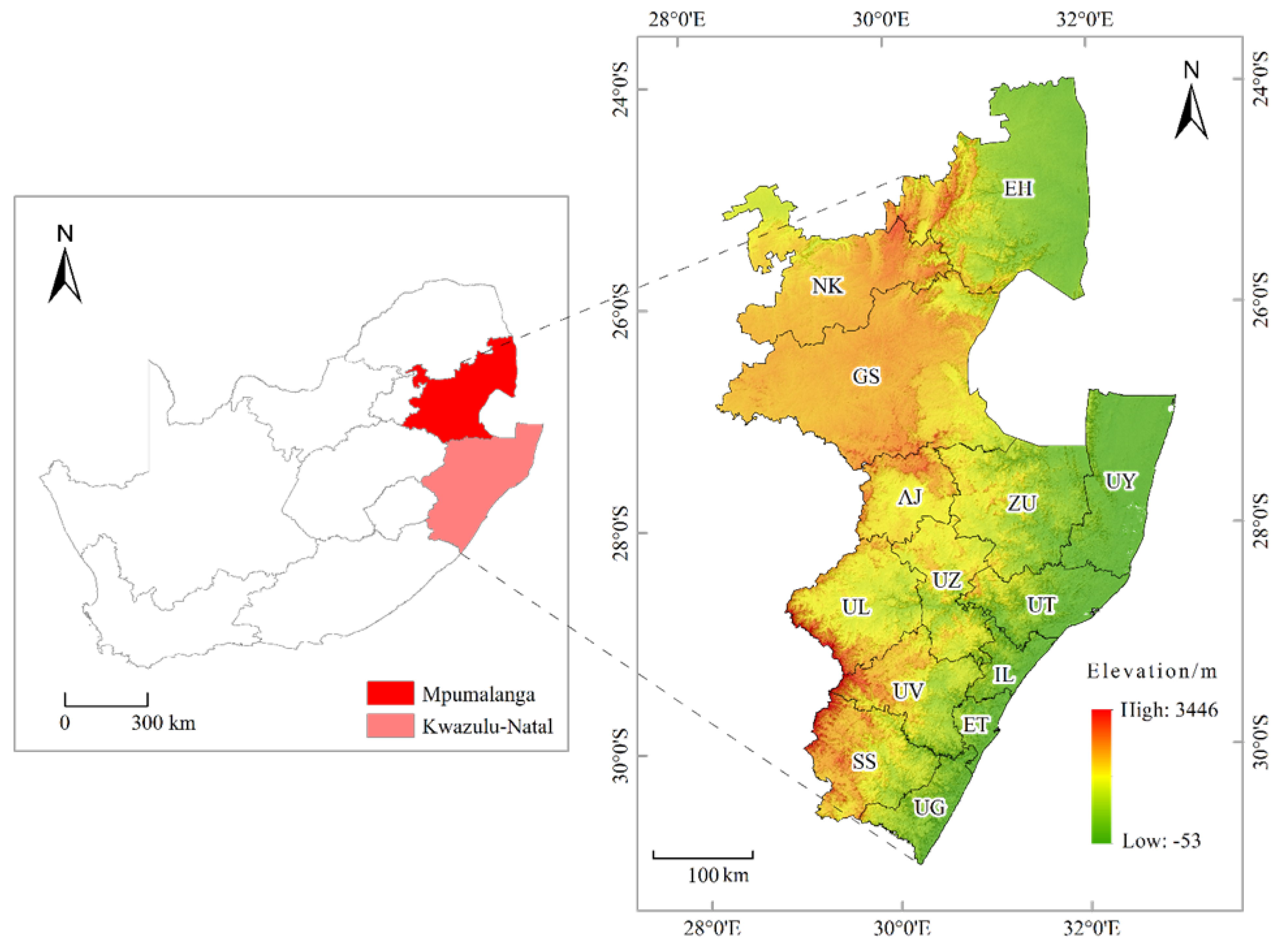
2.1. Study Area

Mpumalanga and KwaZulu-Natal are located in the eastern part of South Africa and hold crucial positions in the overall development of the Republic of South Africa. The total area of the study area is 166,570 km², comprising 14 municipalities and 69 local municipalities. The geographical range is from 24.00°S to 31.08°S and 28.24°E to 32.89°E, with altitudes varying between 0 and 3495 m. The terrain is highly undulating and complex, as illustrated in Figure 1. The region features a diverse climate, with Mpumalanga Province primarily experiencing a tropical grassland climate and KwaZulu-Natal Province predominantly characterized by a temperate marine climate. The annual average temperature in the study area is between 16 and 23 °C, and the precipitation decreases from east to west and from the coast to the interior, ranging between 510 and 1270 mm. The population is primarily comprised of South African black people, with respective population numbers of 13,127,268 in Mpumalanga and 11,278,513 in Kwazulu-Natal. Economically, agriculture, forestry, mining, and tourism are the dominant sectors, with corn, wheat, sugarcane, and fruit as the main crops. Despite the region’s abundant natural resources and favorable ecological environment, activities such as excessive urban expansion, deforestation, land reclamation, coal mining, and the development of tourist areas have led to severe environmental pollution issues. Ecosystems and biodiversity are under significant threat.

2.2. Data Sources

The research data included remote sensing imagery data, topographic data, precipitation data, land surface temperature data, population density data processed through spatial visualization, nighttime light data, and vector data of administrative boundaries at all levels in South Africa (

Table 1. Specific parameters of the research data.

Type	Name	Resolution (m)	Data Source	Notes
Basic data	Administrative boundary	Vector data	https://gadm.org/data.html (accessed on 16 July 2023)
Image data	Landsat5 TM	30	LANDSAT/LT05/C02/T1_L2	1995–2010
	Landsat8 OLI	30	LANDSAT/LC08/C02/T1_L2	2015–2020
Topographic data	NASA-SRTM	30	USGS/SRTMGL1_003
Precipitation data	CHIRPS	5566	UCSB-CHG/CHIRPS/DAILY
LST data	MOD21A1D	1000	MODIS/061/MOD21A1D	2000–2020
Population density data	GPWv411	927.67	CIESIN/GPWv411/GPW_Population_Density
Nighttime light data	DMSP-OLS	927.67	NOAA/DMSP-OLS/CALIBRATED_LIGHTS_V4	1995–2010
	VIIRS	463.83	NOAA/VIIRS/DNB/MONTHLY_V1/VCMSLCFG	2015–2020

Notes: Apart from the basic data, the sources of other data are represented by their data collection ID in GEE, which can be retrieved and acquired from the Earth Engine Data Catalog. The LST data for 1995 were generated by the SMW in conjunction with Landsat 5 imagery.

). Aside from the vector data of South African administrative boundaries, the raster data were obtained on the Google Earth Engine (GEE) platform and were processed in conjunction with GEE and other software such as ArcGIS 10.8 and ENVI 5.6, with all raster data resampled to 30 m. In addition, the temporal range of the MOD21A1D dataset, which provides land surface temperature (LST) information, lacked data for the year 1995, so the LST data for this year were obtained using the statistical mono-window (SMW) algorithm.

3. Methods

3.1. LULC Classification System and Sampling Scheme

(1)

LULC classification system: Regional LULC can be divided based on various classification systems, depending on the application objectives. For example, the International Geosphere-Biosphere Programme (IGBP) system is particularly comprehensive, offering 17 primary classes that range from various types of forests and shrublands to urban and constructed lands [24]. This system is widely recognized for its utility in remote sensing applications and has been adopted in numerous global and regional studies. Studies centered on agriculture may find the Food and Agriculture Organization (FAO) system more fitting [25]. However, it is crucial to recognize that specific research objectives might require different LULC classification systems. For instance, Ge and colleagues divided land use types into farmland, forest, grassland, garden land, residential and industrial land, transportation land, water, and others in their study [26]. Ju divided the LULC into 31 classes when studying the portrayal of the national land use spatial pattern [27]. Given the objectives and the actual situation of the study area, farmland, forest, grassland, water, constructed land, and unused land were adopted as six primary classes for the classification system in this study.

(2)

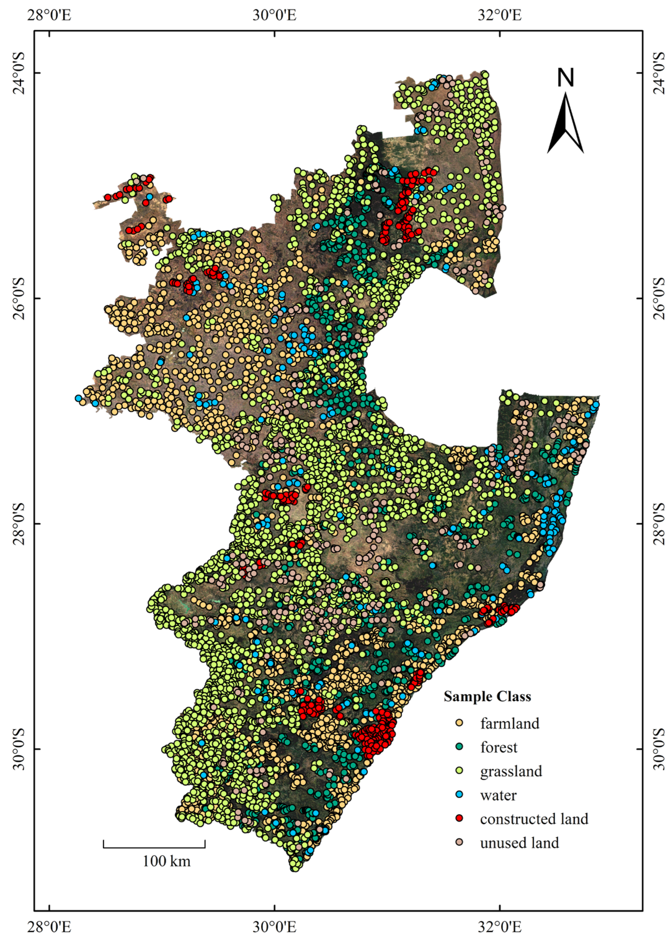
Sampling scheme: In this study, a proportional stratified random sampling method was employed to select training and testing samples for different LULC classes based on their respective area ratio to the total area of the study area [28]. The sampling process was conducted through the visual interpretation of high-resolution imagery available on the GEE platform. A total of 7000 samples were collected across the study area, as illustrated in

Table 2. The land use classification system adopted in this study.

LULC Class	Training Sample	Testing Sample
Farmland	1500	600
Forest	700	280
Grassland	2000	800
Water	200	80
Constructed land	300	120
Unused land	300	120

. The distribution of samples varies depending on the research year under consideration. The distribution map of samples collected for 2020 is shown in Figure 2. It is noteworthy that the samples were collected from individual pixels, thereby ensuring a high level of representativeness for each LULC class. The random division of samples into training and testing sets followed a fixed ratio of 5000 to 2000. Specifically, within each class, the division between training and testing sets maintained a fixed ratio of 5:2.

In the case of object-oriented classification, the sampling process was implemented after the image segmentation phase, utilizing eCognition Developer 9.0 as the software platform. Unlike the pixel-based approach, the sampling unit was the object generated from the segmentation process. A total of 7000 samples were collected independently and were randomly divided into 5000 training samples and 2000 testing samples. The same proportional stratified random sampling method as in the pixel-based approach was adopted, preserving the existing area ratio for different LULC classes. The random division between training and testing sets adhered to the established 5:2 ratio within each class. This maintained methodological consistency across both pixel-based and object-oriented approaches.

3.2. Feature Combination

In the process of remote sensing image classification, choosing an appropriate combination of features can help to maximize the differentiation of various LULC classes, thereby effectively improving classification accuracy [29,30,31]. In this study, the visible, near-infrared, and shortwave infrared bands of Landsat imagery (B1–B5 and B7 bands for L5, B2–B7 bands for L8) were used as spectral features. Four spectral index features, namely the normalized difference vegetation index (NDVI), modified normalized difference water index (MNDWI), normalized difference built-up index (NDBI), and bare soil index (BSI), were generated based on the imagery of each year. By importing NASA-SRTM data, elevation and slope were generated as topographic features. All the features above form the feature combination used for pixel-based classification. The formulas for four spectral indices are as follows:

$$NDVI=\frac{(NIR-RED)}{(NIR+RED)}$$

(1)

$$MNDWI=\frac{(GREEN-MIR)}{(GREEN+MIR)}$$

(2)

$$NDBI=\frac{(SWIR-NIR)}{(SWIR+NIR)}$$

(3)

$$BSI=\frac{(MIR+RED)-(NIR+BLUE)}{(MIR+RED)+(NIR+BLUE)}$$

(4)

where BLUE refers to the blue band, GREEN refers to the green band, RED refers to the red band, NIR refers to the near infrared band, MIR refers to the middle infrared band, and SWIR refers to the short-wave infrared band.

In the object-oriented classification process, in addition to the aforementioned feature combination, texture features generated by the gray-level cooccurrence matrix (GLCM) were added [29]. A GLCM can identify the spatial relationships of pixels in the image, thus calculating the texture features of the objects. Through the GEE platform, the GLCM generates the eight most typical texture features: energy (angular second moment), contrast, correlation, entropy, variance, inverse difference moment, sum average, and dissimilarity.

To reduce the dimensionality of eight texture features, principal component analysis (PCA) was employed. This analysis was conducted using ENVI 5.6 software, which utilizes an orthogonal rotation method for component extraction. Prior to PCA, all original features were subjected to standardization, and the correlation matrix was used for the following analysis. The eigenvalues of the first and second principal components were found to be 4.43 and 1.50, respectively. When considered against the aggregate eigenvalue sum of 6.509, these two components account for over 90% of the total variance, thus serving as an effective representation of the texture information. The component matrix is shown in

Table 3. Component matrix generated from PCA.

Feature	Eig. 1	Eig. 2
Energy	0.396	−0.415
Contrast	−0.396	−0.397
Correlation	−0.154	−0.062
Entropy	−0.409	0.386
Variance	−0.389	−0.425
Inverse difference moment	0.392	−0.365
Sum average	0.049	0.366
Dissimilarity	−0.433	−0.265

, elucidating how each original variable contributes to these principal components [32].

Among all the texture features, energy, contrast, entropy, variance, inverse difference moment, sum average, and dissimilarity primarily contribute to the first and second principal components according to their loadings.

Additionally, the size and shape of the segmented objects were calculated as geometric features to be added to the feature combination for object-oriented classification. The features required for pixel-based classification and object-oriented classification are shown in

Table 4. Features required for pixel-based and object-oriented classification.

Features	Pixel-Based Classification	Object-Oriented Classification
Spectral feature	Landsat8 B2–B7 for 2015 and 2020, Landsat5 B1–B5 and B7 for 1995–2010
Spectral index feature	NDVI, MNDWI, NDBI, BSI
Topographical feature	Elevation, slope
Texture feature	-	Two principal components of features generated from GLCM
Geometrical feature	-	Size, shape

.

3.3. Random Forest Classifier

Random forest classification is an ensemble learning algorithm that performs classification by constructing multiple decision trees. This algorithm randomly draws several subsets from the original training dataset without replacement, with each subset used to build an independent decision tree. Each sample to be classified is input into each decision tree, the prediction results are collected and statistically analyzed, and the class that appears the most times is chosen as the classification output [33]. The random forest classification algorithm has good generalization ability and stability, can effectively handle high-dimensional data, and has strong robustness against noise and outliers, so it is widely used in the field of LULC classification. In addition, the random forest classification algorithm has fast training speed and high accuracy, outperforming many other classification methods. In practical applications, it is important to choose the appropriate size of the subset and the number of decision trees, as these hyperparameters will significantly affect the performance and generalization ability of the model. To optimize the classification process, cross-validation can be used for tuning hyperparameters [34].

3.4. Classification Stage

3.4.1. Pixel-Based Classification

Pixel-based classification operates directly on individual pixels of remote sensing images. In this study, pixel-based classification was executed on the GEE platform. A total of 5000 out of 7000 pixels were selected as training samples through proportional stratified random sampling. The feature set employed for classification encompassed spectral features, spectral index features, and topographic features, focusing on pixel-level information. The random forest classifier was utilized to perform classification, yielding the pixel-based classification outcome.

3.4.2. Object-Oriented Classification

Object-oriented classification uses image segmentation technology to group all pixels in remote sensing images into completely covered and compactly connected objects based on spectral/spatial similarity. In this study, object-oriented classification was performed on eCognition Developer 9.0. A multiscale segmentation method was adopted, assigning equal weight to each feature in the feature combination with a scale setting of 150, and both shape and compactness were set to 0.5 [35]. 5000 out of 7000 total object samples were divided as training samples by proportional stratified random sampling, and a feature combination that included spectral features, topographic features, spectral index features, texture features, and geometric features was used as the basis for classification. The classification was completed using the random forest classifier, resulting in the object-oriented classification outcome [36].

3.5. Optimal Parameter-Based Geodetector

The OPGD model is an improvement of the traditional geographic detector model, comprising five major modules: parameter optimization, factor detection, interaction detection, risk detection, and ecological detection [22]. Traditional studies often yield poor analytical outcomes due to the reliance on experience to group independent variables or the use of a single discretization method across different independent variables. The parameter optimization module addresses this problem by quantitatively evaluating each independent variable, achieving the optimal detection effect on the degree to which each driving factor affects the spatial distribution of the dependent variable. The parameter optimization module can utilize various data grouping methods based on the characteristics of the data (this paper selected four grouping methods: natural breaks method, quantile method, equal distance interval method, and geometric interval method) and set various breakpoint numbers to discretize the independent variables. Moreover, it calculates the q-value for each combination of the grouping method and the breakpoint number. The combination with the highest q-value is selected as the optimal data discretization scheme.

Based on the optimal grouping scheme obtained from the parameter optimization module, the factor detection and interaction detection modules in the OPGD were used to analyze the driving forces of LULCC in the study area. The calculation formula for the factor detection module is as follows:

$$q=1-{\displaystyle \sum _{h=1}^L\frac{N_h{\sigma }_h^2}{N{\sigma }^2}}=1-\frac{SSW}{SST}$$

(5)

$$SSW={\displaystyle \sum _{h=1}^L{N}_h{\sigma }_h^2}$$

(6)

$$SST=N{\sigma }^2$$

(7)

where SSW is the sum of the variances of the dependent variables within the groups corresponding to the discretized independent variables, and SST is the total variance of the dependent variables within the entire area. L is the number of groups for the independent variables, h is the index of the group number, $N_h$ is the number of units of the dependent variables in the h-th group, and N is the number of units of the dependent variables in the entire area. Correspondingly, ${\sigma }_h$ is the variance of the dependent variables in the h-th group, and σ is the variance of the dependent variables in the entire area. q represents that the spatial distribution of the independent variables can explain 100 × q% of the spatial distribution of the dependent variables, and the range of the q-value is [0, 1]. q = 1 indicates that the variance of the dependent variables within the group is 0, which means the distribution of the dependent variables completely matches the distribution of this independent variable, and this independent variable can completely explain the spatial distribution of the dependent variables; in contrast, q = 0 indicates that this independent variable offers no explanation for the spatial distribution of the dependent variables.

3.6. Selection of Dependent Variables and Driving Factors

In the process of driving force analysis, the comprehensive index of land use intensity was selected as the dependent variable for analysis. This index serves as a robust indicator of LULCC, effectively linking LULCC to diverse driving factors that contribute to its dynamics. Considering the natural and socioeconomic characteristics of the study area, as well as the accessibility and comprehensiveness of data coverage over time, the human impact index (HII), population density, total population, nighttime light intensity, elevation, slope, terrain roughness, annual precipitation, surface temperature, and vegetation index were selected as driving factors. The expression of the comprehensive index of land use intensity is as follows:

$$L=100\times {\displaystyle \sum _{i=1}^n{A}_i\times C_i}$$

(8)

where L is the comprehensive index of land use intensity in a specific area, A is the grading index of the degree of land use for the i-th class, C is the ratio of the area of the i-th class of LULC to the total area of the region, and n is the number of LULC classes. In this study, LULC was divided into six classes. Drawing on past research results, the grading indices for farmland, forest, grassland, water, constructed land, and unused land were 3, 2, 2, 2, 4, and 1, respectively [37].

The expression of the HII is as follows:

$$HII={\displaystyle \sum _{i=1}^N\frac{A_i{P}_i}{TA}}$$

(9)

where HII is the human impact index; A is the area of the i-th class of land use; TA is the total area of the region; P is the intensity coefficient of human impact represented by the i-th class of land use; and N is the number of LULC classes. In line with previous research, the coefficients of impact intensity were obtained by averaging the values from the Lohani checklist method, the Leopold matrix method, and the Delphi method. The impact intensity coefficients for farmland, forest, grassland, water, constructed land, and unused land were 0.59, 0.13, 0.10, 0.14, 0.94, and 0.06, respectively [38]. This averaging approach aimed to capture the complementary strengths and mitigate the individual limitations of each method, thus offering a comprehensive and reliable assessment of impact intensities across different land classes.

4. Experimental Results

4.1. Accuracy Assessment

As shown in

Table 5. Accuracy verification of classification results for each year in the study area.

Year	Pixel-Based		Object-Oriented
	OA (%)	KAPPA	OA (%)	KAPPA
1990	62.33%	0.5480	81.67%	0.7800
1995	63.90%	0.5669	85.95%	0.8314
2000	65.52%	0.5863	87.05%	0.8446
2005	68.10%	0.6171	89.33%	0.8720
2010	67.38%	0.6086	89.05%	0.8686
2015	68.68%	0.6242	88.34%	0.8601
2020	72.14%	0.6657	90.57%	0.8869

, among the classification results, the object-oriented classification yielded the best results, with an overall accuracy ranging between 81.67% and 90.57% and a kappa coefficient between 0.7800 and 0.8869. However, the results generated from pixel-based classification were much lower, with an overall accuracy between 62.33% and 72.14% and a kappa coefficient between 0.5480 and 0.6657. Therefore, we decided to employ the object-oriented classification algorithm to extract the LULC data of the study area from 1995 to 2020, followed by post-classification processing, temporal consistency checks, and logical consistency checks. Expert validation and ground-truth validation were applied to rectify any inconsistencies and inaccuracies in the classification, eventually generating the regional LULC dataset (Figure 3).

4.2. LULCC Analysis

According to the multiyear LULC spatial distribution maps of the study area (Figure 3), the temporal change graph of the area proportion of each LULC from 1995 to 2020 could be calculated (Figure 4). According to Figure 3, farmlands were mainly distributed in the southeastern coastal areas and the central-northern plateau regions; grasslands were located primarily in Kruger National Park in the northeast; forests extended north–south along the main mountain ranges within the region; and water, constructed lands, and unused lands were scattered throughout the entire study area. Since 1995, the proportion of farmland has shown a fluctuating upward trend, rising from 28.67% in 1995 to 30.65% in 2000, then declining to 29.45% in 2005, subsequently increasing gradually and reaching a peak in 2015 at 31.40% of the total area before falling to 30.95% in 2020. This trend might be related to proactive measures taken by the local government in agricultural policy, food security, and productivity enhancement. The proportion of forest decreased from 15.08% in 1995 to 13.50% in 2020. This decline could be attributed to unsustainable exploitation of forest resources, illegal logging, and related activities. Despite the local government’s efforts in forest conservation, significant challenges persist in implementation. Similarly, the proportion of grassland showed a downward trend, dropping from 49.80% in 1995 to 43.21% in 2020. This decline could be associated with the expansion of agricultural land, accelerated urbanization, and infrastructure development. The proportion of water bodies fluctuated over the 25-year period, peaking at 1.09% in 2000 and reaching a low of 0.73% in 2005. This variation might be linked to intensified efforts by the local government in water resource management as well as the influence of natural factors such as annual fluctuation and climate change. The proportion of constructed land consistently increased throughout the study period, growing from 2.88% in 1995 to 6.08% in 2020, with a growth rate of 111.1%. This reflects the rapid socio-economic and urbanization developments in the study area. The accelerated growth rate in constructed land indicates increased investment in infrastructure and commercial activities, which in turn have attracted a larger population to the region. Additionally, this trend aligns with the government’s strategic focus on urban planning, aimed at fostering economic prosperity and improving the quality of life for residents. The proportion of unused land fluctuated during the study period, dropping from 2.82% in 1995 to 2.19% in 2000, then gradually rising to 5.97% in 2015 and declining to 5.31% in 2020. This fluctuation might result from adjustments in land resource policies as well as the impact of natural disasters [39].

4.3. Driving Force Analysis

4.3.1. Parameter Optimization

The best discretization schemes for the ten driving factors, derived from the built-in Geographical Detector Model (GDM) function in OPGD, are presented in

Table 6. Optimal discretization method and optimal number of categories of the selected variables.

Independent Variable	1995		2000		2005		2010		2015		2020
	Method	BK	Method	BK	Method	BK	Method	BK	Method	BK	Method	BK
HII	natural	11	natural	12	natural	12	natural	11	geometric	10	geometric	12
PD	quantile	11	quantile	9	quantile	11	quantile	12	quantile	11	quantile	11
POP	quantile	11	natural	8	quantile	11	quantile	9	natural	8	quantile	10
NIG	quantile	8	quantile	9	natural	9	quantile	12	quantile	12	quantile	12
ELE	equal	12	equal	12	equal	12	equal	12	equal	12	equal	12
SLO	natural	11	natural	11	natural	11	natural	11	natural	11	natural	11
REL	natural	12	natural	12	natural	12	natural	12	natural	12	natural	12
PRE	quantile	10	natural	12	quantile	12	quantile	12	natural	12	geometric	12
LST	quantile	10	natural	12	natural	11	quantile	9	quantile	12	quantile	12
NDVI	equal	10	natural	10	natural	11	natural	12	quantile	11	quantile	10

Notes: (1) The column labeled “BK” stands for the number of breakpoints. (2) HII stands for human impact index; PD stands for population density; POP stands for total population; NIG stands for nighttime light intensity; ELE stands for elevation; SLO stands for slope; REL stands for terrain roughness; PRE stands for annual precipitation; LST stands for surface temperature; and NDVI stands for normalized difference vegetation index. (3) Natural stands for natural breaks method; quantile stands for quantile method; equal stands for equal distance interval method; geometric stands for geometric interval method.

. Among these factors, elevation, slope, and terrain roughness were three static driving factors that described topographic features that were not affected by temporal changes. Moreover, the optimal grouping methods and breakpoint numbers varied for different independent variables and even for the same variable across different years, underscoring the spatiotemporal variations of these variables. By employing the optimal discretizing method, each independent variable can be assured of having a high q-value, emphasizing their potential significance. This method also ensures significant differences between each group, precisely indicating the extent of influence each independent variable has on the spatiotemporal differentiation of the dependent variable.

4.3.2. Factor Detection

By selecting the optimal discretization scheme for each year and using the GDM function for factor detection and interaction detection, we obtained the degree of influence on the annual comprehensive index of land use intensity by socioeconomic factors, including the human impact index (HII), population density (PD), total population (POP), and nighttime light intensity (NIG), as well as natural factors, including the elevation (ELE), slope (SLO), terrain roughness (REL), annual precipitation (PRE), surface temperature (LST), and vegetation index (NDVI) (

Table 7. Factor detection results of the land use intensity index in the study area from 1995 to 2020.

Factors	1995		2000		2005		2010		2015		2020
	q-Value	p-Value	q-Value	p-Value	q-Value	p-Value	q-Value	p-Value	q-Value	p-Value	q-Value	p-Value
HII	0.971	7.41 × 10−10	0.977	5.55 × 10−10	0.976	3.41 × 10−10	0.974	9.94 × 10−10	0.964	6.29 × 10−10	0.970	3.52 × 10−10
PD	0.317	1.74 × 10−10	0.518	9.85 × 10−10	0.672	7.91 × 10−10	0.614	5.11 × 10−10	0.650	2.57 × 10−10	0.657	3.15 × 10−10
POP	0.166	2.61 × 10−10	0.214	3.94 × 10−10	0.232	3.78 × 10−10	0.185	4.34 × 10−10	0.160	3.77 × 10−10	0.141	2.75 × 10−9
NIG	0.374	6.46 × 10−10	0.527	5.93 × 10−10	0.665	3.14 × 10−10	0.630	9.27 × 10−10	0.687	8.31 × 10−10	0.688	5.91 × 10−10
ELE	0.135	7.79 × 10−11	0.095	9.57 × 10−10	0.127	2.15 × 10−10	0.107	2.62 × 10−10	0.111	3.91 × 10−8	0.089	6.82 × 10−10
SLO	0.039	4.42 × 10−7	0.086	4.74 × 10−10	0.111	3.24 × 10−10	0.154	6.48 × 10−10	0.178	6.75 × 10−10	0.158	5.61 × 10−10
REL	0.059	2.67 × 10−6	0.107	6.27 × 10−10	0.135	1.73 × 10−10	0.172	3.15 × 10−10	0.202	4.32 × 10−10	0.177	3.81 × 10−10
PRE	0.049	4.18 × 10−2	0.053	1.04 × 10−10	0.041	2.41 × 10−2	0.034	6.05 × 10−1	0.095	3.35 × 10−5	0.110	7.32 × 10−10
LST	0.053	2.06 × 10−6	0.099	1.19 × 10−5	0.133	7.63 × 10−10	0.064	3.48 × 10−5	0.071	4.26 × 10−1	0.140	3.75 × 10−10
NDVI	0.124	5.85 × 10−6	0.193	8.88 × 10−10	0.115	9.68 × 10−10	0.160	9.28 × 10−10	0.109	4.50 × 10−10	0.197	4.88 × 10−10

).

As seen in Table 7, the explanatory power of socioeconomic factors was generally higher than that of natural factors. The explanatory power of the human impact index was the highest, with a stable q-value of approximately 0.97 between 1995 and 2020, indicating that human activities, including increased urbanization, agricultural expansion, and industrial development, played a decisive role in LULCC. The explanatory power of population density and nighttime light intensity was relatively high, with the q-value of population density peaking in 2005 at 0.672 and the q-value of nighttime light intensity peaking in 2020 at 0.688. High explanatory power signifies the substantial impact of these two driving factors on LULCC. Nighttime light intensity serves as a compelling proxy for economic activity, urbanization, and technological advancement. It is directly correlated with the level of industrialization and the proliferation of services that operate during nighttime hours [40]. On the other hand, high population density often necessitates more intensive land use, whether for housing, transportation, or public services. The explanatory power of the total population was relatively weak, with the highest q-value occurring in 2005, at 0.232. The relatively low explanatory power of the total population suggests that it is not merely the number of people that matters, but how they are distributed and what activities they are engaged in.

The explanatory power of natural factors for LULCC in this region was relatively low, with the highest explanatory power not exceeding 0.202 during the study period. This indicates that the impact of natural factors on the degree of land use was not as significant as that of human activities. Among these factors, the explanatory power of topographic factors was greater than that of climate factors, with the average explanatory power of topographic factors and climate factors during the study period being 0.125 and 0.102, respectively. Among the topographic factors, the explanatory power of terrain roughness was higher than that of elevation and slope except in 1995, with the highest q-value being 0.202 in 2015. The explanatory power of elevation and slope alternately led during the study period, with the highest q-value of elevation occurring in 1995 at 0.135 and the highest q-value of slope occurring in 2015 at 0.178. It indicates that topographical factors play a pivotal role in determining the feasibility of various land use types, thus affecting LULCC. For instance, elevation serves as a constraint for agricultural activities, as higher altitudes may not be conducive to certain crops. Similarly, slope restricts the range and viability of construction projects, as it requires more sophisticated engineering solutions for steeper terrains. Terrain roughness, on the other hand, might influence both agriculture and development, as uneven landscapes may necessitate specialized land management practices [41]. Among the three factors representing climate and vegetation, the explanatory power of the vegetation index was generally higher, with the highest q-value being 0.197 in 2020. This could be due to the role of vegetation variation in soil stabilization and water retention, which are critical for both natural ecosystems and human activities. The highest q-values for annual precipitation and surface temperature both occurred in 2020, at 0.110 and 0.140, respectively. Although annual precipitation and surface temperature are often considered key indicators of climate and its impact on LULCC, the response speed of features to climate condition changes is usually not significant in a short period of time. Therefore, the explanatory power of annual precipitation and surface temperature was relatively low.

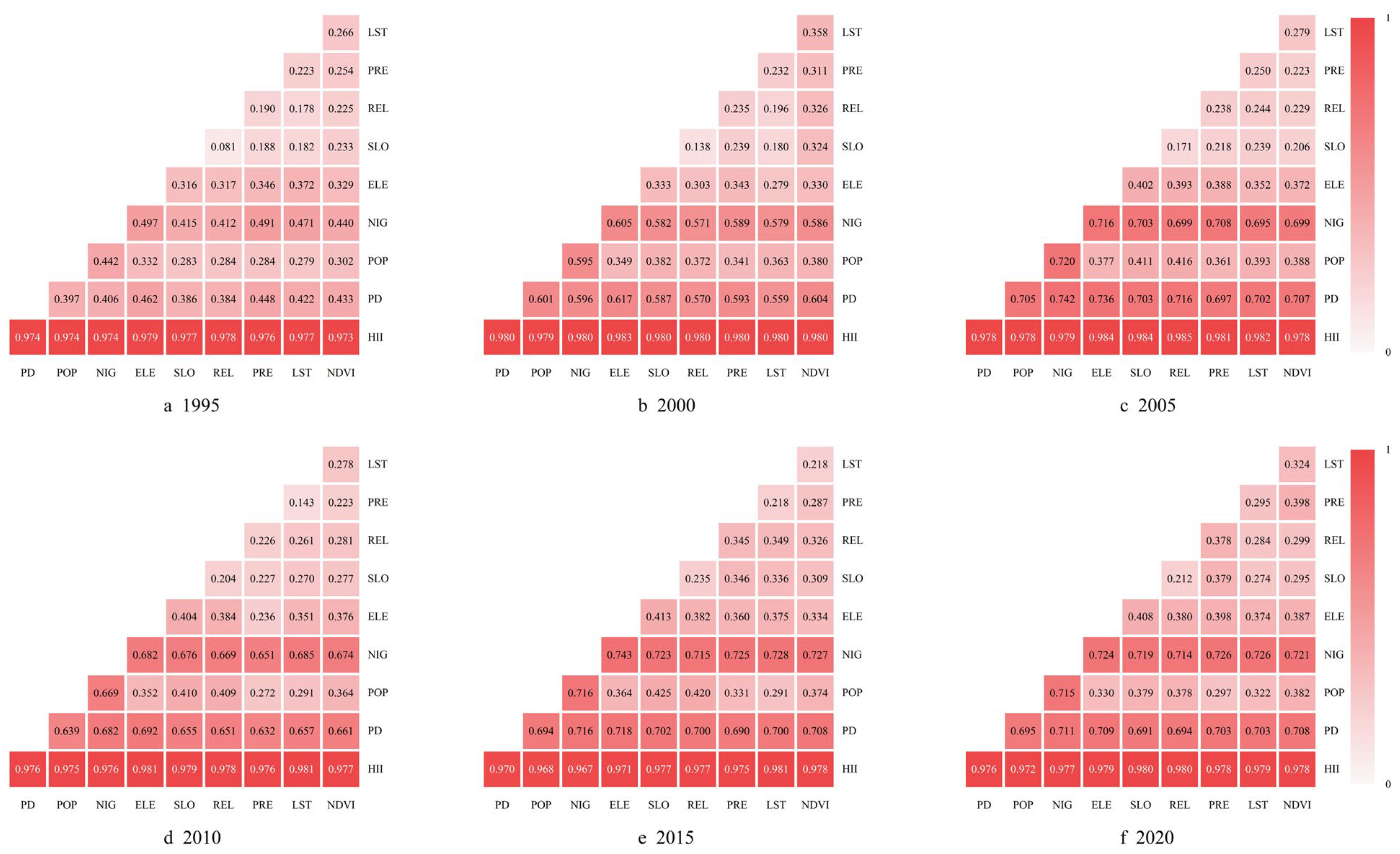
4.3.3. Interaction Detection

The interactions between the 10 driving factors are shown in Figure 5. During the study period, the q-values of the HII and any other driving factor remained between 0.968 and 0.985 after interaction, demonstrating extremely high explanatory power. Each selected driving factor showed a dual-factor enhancement effect when coupled with the HII. Apart from the HII, the interaction of nighttime light intensity and population density with other factors showed enhanced effects. Among them, the coupling of nighttime light intensity with other factors yielded higher q-values. The coupling relationships of these two driving factors with others showed dual-factor enhancement and nonlinear enhancement, and the specific coupling situations varied according to different years and conditions. Notably, in 2015, the interaction between nighttime light intensity and elevation showed the strongest explanatory power, reaching 0.743, suggesting that as elevation rises, urbanization tends to decrease, thereby influencing LULCC in ways particularly relevant to human interference. In other years, the interaction between the two was relatively strong, showing dual-factor enhancement effects. This result indicates that socioeconomic development at various altitudes was the main driving factor influencing the spatial differentiation of land use intensity in each year. The coupling of the remaining driving factors involved dual-factor enhancement or nonlinear enhancement relationships, with the factors interdependent and without any mutual inhibition. The weakest interaction combinations were slope and terrain roughness in 1995, 2000, 2005, and 2020, while in 2010 and 2015, the weakest interaction was between annual precipitation and surface temperature. These results indicated that when natural factors were coupled, the intensity of their influence on LULCC was lower than that of the influence exerted by the coupling of natural and socioeconomic factors and the coupling among socioeconomic factors. This might be due to the more direct and immediate impact that socioeconomic activities often have on LULCC compared to the generally slower changes induced by natural factors.

5. Discussion

5.1. Comparison of Accuracy Difference of Classification Methods

This study applied two distinct classification methods to classify the LULC of the study area and created a spatial distribution map of the LULC every five years from 1995 to 2020. However, the accuracy of pixel-based classification did not meet the threshold required for the following research. In contrast, the object-oriented classification added texture features and geometric features on the basis of spectral features, spectral index features, and topographic features, which jointly trained the classifier. This enabled the integration of a richer set of information in the feature space of the sample data, significantly improving the classification effect, and the overall accuracy was maintained above 80%. Although numerous studies have indicated that object-oriented classification exhibits clear advantages when processing high-resolution imagery, with the ability to effectively remove salt-and-pepper noise and better identify ambiguous land cover types and transition boundaries, this study found that object-oriented classification also contributed to high-precision classification results when handling Landsat series satellite imagery with a spatial resolution of 30 m [42,43,44]. It could achieve a good balance between overrefinement and overgeneralization, which aligns with the research findings of Tassi et al. [16]. Additionally, according to the classification results and visual interpretation verification, the primary LULC class in Kruger National Park, located in the northeastern part of the study area, was grassland. However, research by Liu et al. indicated that Kruger National Park has been largely occupied by constructed land, suggesting that there is a certain bias in the LULC data derived from relying on a single classification method [45]. In practical research, to circumvent issues with insufficient classification accuracy from a single method, multiple classification methods can be employed and compared, with the highest accuracy scheme selected, to obtain more precise LULC classification data. This strategy not only enhances the reliability of LULC classification data but also ensures the accuracy and effectiveness of following driving force studies. Moreover, adopting various classification methods for comparison and optimization helps to reveal the strengths and weaknesses of different methods under various geographic environments and parameter settings, providing useful references for future studies.

5.2. Primary Driving Factors of LULCC

The analysis results of LULCC driving forces suggest that socioeconomic activities often have a greater impact on LULC than natural processes do. This result is consistent with the research conclusions of Wang et al. and Long et al., who emphasized that socioeconomic factors played a more crucial role in LULCC. Among the socioeconomic factors, nighttime light intensity can reflect the strength and distribution of regional GDP to a certain degree. Economically developed regions tend to have a high degree of urbanization and population aggregation, contributing to high land use intensity. From 1995 to 2020, the population in the study area increased from 11,217,732 to 24,405,781. The population surge led to rapid expansion of construction and residential land, thereby accelerating changes in the LULC distribution pattern. The influence of natural factors was relatively low, with topographic factors having a greater impact than climatic factors. To a certain extent, the variations in the terrain restrict or promote the progress of human activities and regulate the distribution of water, heat, and plants. Elevation affects atmospheric pressure, temperature, relative humidity, and the vertical distribution of vegetation, while slope determines the stability and difficulty of development. Therefore, topographic indicators have an impact on LULCC that cannot be ignored. The natural conditions like climate patterns, topography, and resource endowment in KwaZulu-Natal and Mpumalanga Provinces restrict the exercise of human subjective initiative, while human activities, in turn, change the appearance, characteristics, functions, and quality of the local natural environment. LULCC is one of the important manifestations of the interaction between nature and humans. In the long term, natural factors have a greater impact on the degree of land use; however, in the short term, socioeconomic activities within human settlements bring more significant changes to and influences on land use.

Policy factors within socioeconomic factors also have a significant impact on LULCC. After the abolition of apartheid in 1994, South Africa implemented a series of urbanization reform policies to promote urban development, reduce poverty and inequality, improve quality of life, and protect the ecological environment. These policies covered diverse aspects, such as urban renewal and regeneration, urban-rural integration, urban governance, and urban participation. Due to these policies, the proportion of the urban population in the region increased from 62.1% in 2010 to 66.3% in 2019, leading to a rapid expansion of constructed land. South Africa’s urbanization reform policies have significantly impacted LULCC, revealing many pressing issues that need to be resolved, including: ① urban expansion under policy guidance has led to the reduction of agricultural land, loss of rural population, and a decline in agricultural production capacity; ② an inadequate land management system has led to unclear land ownership, frequent land disputes, and severe wastage of land resources; and ③ haphazard land use planning has exacerbated environmental problems such as soil erosion, water pollution, and biodiversity loss.

Furthermore, with the implementation of the National Environmental Management Act in 1998, South Africa began enforcing biodiversity protection policies aimed at preserving its unique and rich biological resources. Measures such as establishing nature reserves, formulating ecosystem management plans, and promoting the concept of sustainable development to minimize damage to the ecological environment. KwaZulu-Natal and Mpumalanga provinces, among the richest in South Africa in terms of biodiversity and natural landscapes, have established various reserves, such as Kruger National Park, Bladen Nature Reserve, and St. Lucia Wetland Park. This policy effectively lowered the degree of land use within these nature reserves, reduced the intensity of human disturbance and development, and maintained stability in forest and grassland cover, thereby enhancing the integrity and stability of the regional ecosystem.

5.3. Prospect and Limitation

The results of the present study significantly impact policy formulation, development planning, and environmental conservation. Building upon the insights gained from this study, forthcoming research will delve deeper into monitoring the evolving trends of LULC and the underlying mechanisms of LULCC. A particularly promising direction for future inquiry is the scenario simulation of LULC dynamics. Such computational models will not only enhance our understanding of the principal driving forces but also provide critical data for informed decision-making, offering scientific guidance for further sustainable land management.

This study still has the following shortcomings: ① When generating the GLCM, the weighting scheme possesses some subjectivity, and this process needs to be refined in future research. ② When analyzing the factors affecting land use intensity, some factors, such as road network density, road area, and distance from roads, are missing. These missing transportation factors may have a certain impact on the results. Future research will obtain more data to analyze the spatiotemporal characteristics and driving factors of LULCC in the study area more comprehensively.

6. Conclusions

This study compared the accuracy of LULC extraction from pixel-based and object-oriented classification methods, selected the optimal classification method to support further LULCC driving force analysis, and drew the following conclusions: ① For the Landsat series of satellite images, the object-oriented classification outperformed the pixel-based approach. The overall accuracy of LULC data from 1995 to 2020 was more than 80%, and the kappa coefficient was more than 78%, which met the requirements of the following research. ② From 1995 to 2020, the area of farmland in the study area fluctuated and increased, while the areas of forest and grassland gradually decreased. The area of constructed land significantly grew, and the areas of water and unused land fluctuated. ③ Socioeconomic factors had a greater impact on LULCC than natural factors. Socioeconomic factors, mainly population growth, economic development, and urban expansion, dramatically increased the demand for farmland and constructed land, accelerating the transition of various land classes toward constructed land and farmland, thereby directly or indirectly affecting regional LULCC. Natural factors primarily lead to LULCC by affecting soil quality, hydrological conditions, vegetation distribution, etc. Due to the longer time scale and larger spatial scale of the influence of natural factors and their interference and regulation by human activities, their impact on LULCC is relatively subtle and slow. ④ This study identified the reasons for LULCC qualitatively and quantitatively, providing a scientific basis for the land planning and management departments in KwaZulu-Natal and Mpumalanga provinces to protect the local ecological environment, comprehensively plan future urbanization processes, and accurately promote sustainable development strategies.

References

1. Abraham, A.; Kundapura, S. Spatio-temporal Dynamics of Land Use Land Cover Changes and Future Prediction Using Geospatial Techniques. J. Indian Soc. Remote Sens. 2022, 50, 2175–2191. [Google Scholar] [CrossRef]
2. Wang, X.; Bao, Y. Study on the Methods of Land Use Dynamic Change Research. Prog. Geogr. 1999, 1, 83–89. [Google Scholar]
3. Hitayezu, P.; Wale, E.; Ortmann, G.F. Assessing Agricultural Land-use Change in the Midlands Region of KwaZulu-Natal, South Africa: Application of Mixed Multinomial Logit. Environ. Dev. Sustain. 2016, 18, 985–1003. [Google Scholar] [CrossRef]
4. Coetzer, K.; Erasmus, B.; Witkowski, E.; Bachoo, K.A. Land-cover Change in the Kruger to Canyons Biosphere Reserve (1993–2006): A First Step towards Creating a Conservation Plan for the Subregion. South Afr. J. Sci. 2010, 106, 1–10. Available online: https://hdl.handle.net/10520/EJC97059 (accessed on 1 October 2023). [CrossRef]
5. Chen, Y.; Yang, P. Recent Progresses of International Study on Land Use and Land Cover Change (LUCC). Econ. Geogr. 2001, 21, 95–100. [Google Scholar]
6. Houghton, R.A. The Worldwide Extent of Land-Use Change. BioScience 1994, 44, 305–313. [Google Scholar] [CrossRef]
7. Haack, B.; Mahabir, R.; Kerkering, J. Remote Sensing-derived National Land Cover Land Use Maps: A Comparison for Malawi. Geocarto Int. 2015, 30, 270–292. [Google Scholar] [CrossRef]
8. Lin, Q.; Eladawy, A.; Sha, J.; Li, X.; Wang, J.; Kurbanov, E.; Thomas, A. Remotely Sensed Ecological Protection Redline and Security Pattern Construction: A Comparative Analysis of Pingtan (China) and Durban (South Africa). Remote Sens. 2021, 13, 2865. [Google Scholar] [CrossRef]
9. Tian, L.; Tao, Y.; Fu, W.; Li, T.; Ren, F.; Li, M. Dynamic Simulation of Land Use/Cover Change and Assessment of Forest Ecosystem Carbon Storage under Climate Change Scenarios in Guangdong Province, China. Remote Sens. 2022, 14, 2330. [Google Scholar] [CrossRef]
10. Fang, J.; Zhu, J.; Wang, S.; Yue, C.; Shen, H. Global Warming, Human-induced Carbon Emissions, and Their Uncertainties. Sci. China Earth Sci. 2011, 54, 1458–1468. [Google Scholar] [CrossRef]
11. Maxwell, A.E.; Warner, T.A.; Fang, F. Implementation of Machine-learning Classification in Remote Sensing: An Applied Review. Int. J. Remote Sens. 2018, 39, 2784–2817. [Google Scholar] [CrossRef]
12. Myint, S.W.; Gober, P.; Brazel, A.; Clarke, S.G.; Weng, Q. Per-pixel vs. Object-based Classification of Urban Land Cover Extraction Using High Spatial Resolution Imagery. Remote Sens. Environ. 2011, 115, 1145–1161. [Google Scholar] [CrossRef]
13. Phan, T.N.; Kuch, V.; Lehnert, L.W. Land Cover Classification Using Google Earth Engine and Random Forest Classifier—The Role of Image Composition. Remote Sens. 2020, 12, 2411. [Google Scholar] [CrossRef]
14. Yan, Y.; Dong, X.; Li, Y. The Comparative Study of Remote Sensing Image Supervised Classification Methods Based on ENVI. Beijing Surv. Mapp. 2011, 3, 14–16. [Google Scholar] [CrossRef]
15. Zhao, C.; Qian, L. Comparative Study of Supervised and Unsupervised Classification in Remote Sensing Image. J. Henan Univ. Nat. Sci. 2004, 34, 90–93. [Google Scholar] [CrossRef]
16. Tassi, A.; Gigante, D.; Modica, G.; Martino, L.; Vizzari, M. Pixel- vs. Object-Based Landsat 8 Data Classification in Google Earth Engine Using Random Forest: The Case Study of Maiella National Park. Remote Sens. 2021, 13, 2299. [Google Scholar] [CrossRef]
17. Wang, J.; Xu, C. Geodetector: Principle and prospective. Acta Geogr. Sin. 2017, 72, 116–134. [Google Scholar]
18. Wang, Z.; Jiang, Y.; Zhang, Y.; Duan, S.; Liu, J.; Zeng, Z.; Zeng, S. Spatial Distribution and Driving Factors of Karst Rocky Desertification Based on GIS and Geodetectors. Acta Geogr. Sin. 2019, 74, 1025–1039. [Google Scholar]
19. Wang, C.; Zhang, J.; Li, H. Spatio-temporal Evolution and Driving Forces of Land Use Patterns in Chongqing City Supported by Multiple Methods. Bull. Soil Water Conserv. 2023, 43, 104–116. [Google Scholar] [CrossRef]
20. Shrestha, N. Detecting Multicollinearity in Regression Analysis. Am. J. Appl. Math. Stat. 2020, 8, 39–42. [Google Scholar] [CrossRef]
21. Zhao, R.; Zhan, L.; Yao, M.; Yang, L. A Geographically Weighted Regression Model Augmented by Geodetector Analysis and Principal Component Analysis for the Spatial Distribution of PM2.5. Sustain. Cities Soc. 2020, 56, 102106. [Google Scholar] [CrossRef]
22. Song, Y.; Wang, J.; Ge, Y.; Xu, C. An Optimal Parameters-based Geographical Detector Model Enhances Geographic Characteristics of Explanatory Variables for Spatial Heterogeneity Analysis: Cases with Different Types of Spatial Data. GIScience Remote Sens. 2020, 57, 593–610. [Google Scholar] [CrossRef]
23. Hu, Q.; Wu, W.; Xia, T.; Yu, Q.; Yang, P.; Li, Z.; Song, Q. Exploring the Use of Google Earth Imagery and Object-Based Methods in Land Use/Cover Mapping. Remote Sens. 2013, 5, 6026–6042. [Google Scholar] [CrossRef]
24. Loveland, T.R.; Reed, B.C.; Brown, J.F.; Ohlen, D.O.; Zhu, Z.; Yang, L.; Merchant, J.W. Development of a global land cover characteristics database and IGBP DISCover from 1 km AVHRR data. Int. J. Remote Sens. 2010, 21, 1303–1330. [Google Scholar] [CrossRef]
25. Gong, P.; Wang, J.; Yu, L.; Zhao, Y.; Zhao, Y.; Liang, L.; Niu, Z.; Huang, X.; Fu, H.; Liu, S.; et al. Finer resolution observation and monitoring of global land cover: First mapping results with Landsat TM and ETM+ data. Int. J. Remote Sens. 2012, 34, 2607–2654. [Google Scholar] [CrossRef]
26. Ge, Q.; Zhao, M.; Zheng, J. Land Use Change in China during 20th Century. Acta Geogr. Sin. 2000, 6, 698–706. [Google Scholar]
27. Ju, H. Method on Describing the Spatial Pattern of Land Use and Its Application in China; University of Chinese Academy of Science: Beijing, China, 2018. [Google Scholar]
28. Shetty, S.; Gupta, P.K.; Belgiu, M.; Srivastav, S.K. Assessing the Effect of Training Sampling Design on the Performance of Machine Learning Classifiers for Land Cover Mapping Using Multi-Temporal Remote Sensing Data and Google Earth Engine. Remote Sens. 2021, 13, 1433. [Google Scholar] [CrossRef]
29. Tassi, A.; Vizzari, M. Object-Oriented LULC Classification in Google Earth Engine Combining SNIC, GLCM, and Machine Learning Algorithms. Remote Sens. 2020, 12, 3776. [Google Scholar] [CrossRef]
30. Lu, D.; Weng, Q. A Survey of Image Classification Methods and Techniques for Improving Classification Performance. Int. J. Remote Sens. 2007, 28, 823–870. [Google Scholar] [CrossRef]
31. Kumar, U.; Dasgupta, A.; Mukhopadhyay, C.; Ramachandra, T.V. Examining the Effect of Ancillary and Derived Geographical Data on Improvement of Per-Pixel Classification Accuracy of Different Landscapes. J. Indian Soc. Remote Sens. 2018, 46, 407–422. [Google Scholar] [CrossRef]
32. Wold, S.; Esbensen, K.; Geladi, P. Principal Component Analysis. Chemom. Intell. Lab. Syst. 1987, 2, 37–52. [Google Scholar] [CrossRef]
33. Fang, K.; Wu, J.; Zhu, J.; Xie, B. A Review of Technologies on Random Forests. J. Stat. Inf. 2011, 26, 32–38. [Google Scholar]
34. Li, X. Using “Random Forest”for Classification and Regression. Chin. J. Appl. Entomol. 2013, 50, 1190–1197. [Google Scholar]
35. Liang, Y. Object-Oriented vs. Pixel-Based Method for Land-Use Classification Using High-Resolution Remote Sensing Images; Taiyuan University of Technology: Taiyuan, China, 2012. [Google Scholar]
36. Liang, L.; Wang, J.; Deng, F.; Kong, D. Mapping Pu’er Tea Plantations from GF-1 Images Using Object-Oriented Image Analysis (OOIA) and Support Vector Machine (SVM). PLoS ONE 2023, 18, e0263969. [Google Scholar] [CrossRef] [PubMed]
37. Wang, S.; Liu, J.; Zhang, Z.; Zhou, Q.; Zhao, X. Analysis on Spatial-Temporal Features of Land Use in China. Acta Geogr. Sin. 2001, 56, 631–639. [Google Scholar]
38. Liang, F.; Liu, L. Quantitative Analysis of Human Disturbance Intensity of Landscape Patterns and Preliminary Optimization of Ecological Function Regions: A Case of Minqing County in Fujian Province. Resour. Sci. 2011, 33, 1138–1144. [Google Scholar]
39. Wessels, K.J.; Reyers, B.; Jaarsveld, A.S.; Rutherford, M.C. Identification of potential conflict areas between land transformation and biodiversity conservation in north-eastern South Africa. Agric. Ecosyst. Environ. 2003, 95, 157–178. [Google Scholar] [CrossRef]
40. Keola, S.; Andersson, M.; Hall, O. Monitoring economic development from space: Using nighttime light and land cover data to measure economic growth. World Dev. 2015, 66, 322–334. [Google Scholar] [CrossRef]
41. Wu, L.; Yang, Y.; Yang, H.; Xie, B.; Luo, W. A Comparative Study on Land Use/Land Cover Change and Topographic Gradient Effect between Mountains and Flatlands of Southwest China. Land 2023, 12, 1242. [Google Scholar] [CrossRef]
42. Cao, X.; Ke, C. Classification of High-resolution Remote Sensing Images Using Object-oriented Method. Remote Sens. Inf. 2006, 5, 27–30. [Google Scholar]
43. Blaschke, T. Object Based Image Analysis for Remote Sensing. ISPRS J. Photogramm. Remote Sens. 2010, 65, 2–16. [Google Scholar] [CrossRef]
44. Benz, U.C.; Hofmann, P.; Willhauck, G.; Lingenfelder, I.; Hynen, M. Multi-resolution, Object-oriented Fuzzy Analysis of Remote Sensing Data for GIS-ready Information. ISPRS J. Photogramm. Remote Sens. 2004, 58, 239–258. [Google Scholar] [CrossRef]
45. Liu, L.; Li, J.; Wang, J.; Liu, F.; Cole, J.; Sha, J.; Jiao, Y.; Zhou, J. The Establishment of An Eco-environmental Evaluation Model for Southwest China and Eastern South Africa Based on the DPSIR Framework. Ecol. Indic. 2022, 145, 109687. [Google Scholar] [CrossRef]
Figure 1. Location and topography of Kwazulu−Natal and Mpumalanga provinces.
Remotesensing 15 04823 g001
Figure 2. Distribution of 7000 samples, taking 2020 as an example.
Remotesensing 15 04823 g002
Figure 3. Spatiotemporal pattern of land use from 1995 to 2020 (derived from object-oriented classification).
Remotesensing 15 04823 g003
Figure 4. Temporal changes in the area occupied by each land use type in the study area from 1995 to 2020.
Remotesensing 15 04823 g004
Figure 5. Interactive detection results of driving force factors during 1995–2020.
Remotesensing 15 04823 g005