Machine Learning-Based Calibrated Model for Forecast Vienna Mapping Function 3 Zenith Wet Delay

Abstract

An accurate estimation of zenith wet delay (ZWD) is crucial for global navigation satellite system (GNSS) positioning and GNSS-based precipitable water vapor (PWV) inversion. The forecast Vienna Mapping Function 3 (VMF3-FC) is a forecast product provided by the Vienna Mapping Functions (VMF) data server based on the European Centre for Medium-Range Weather Forecasts (ECMWF)-based numerical weather prediction (NWP) model. The VMF3-FC can provide ZWD at any time and for any location worldwide; however, it has an uneven accuracy distribution and fails to match the application requirements in certain areas. To address this issue, in this study, a calibrated model for VMF3-FC ZWD, named the XZWD model, was developed by utilizing observation data from 492 radiosonde sites globally from 2019–2021 and the eXtreme Gradient Boosting (XGBoost) algorithm. The performance of the XZWD model was validated using 2022 observation data from the 492 radiosonde sites. The XZWD model yields a mean bias of −0.03 cm and a root-mean-square error (RMSE) of 1.64 cm. The XZWD model outperforms the global pressure and temperature 3 (GPT3) model, reducing the bias and RMSE by 94.64% and 58.90%, respectively. Meanwhile, the XZWD model outperforms VMF3-FC, with a reduction of 92.68% and 6.29% in bias and RMSE, respectively. Furthermore, the XZWD model reduces the impact of ZWD accuracy by latitude, height, and seasonal variations more effectively than the GPT3 model and VMF3-FC. Therefore, the XZWD model yields higher stability and accuracy in global ZWD forecasting.

1. Introduction

Zenith tropospheric delay (ZTD) is a crucial error source in global navigation satellite system (GNSS) positioning. An accurate prior ZTD is beneficial for positioning accuracy and convergence time in precise point positioning (PPP) [1,2,3,4,5,6,7,8,9]. ZTD has two components: zenith hydrostatic delay (ZHD) and zenith wet delay (ZWD) [10]. ZWD is critical for GNSS-based precipitable water vapor (PWV) inversion. PWV is strongly associated with precipitation, extreme weather events (typhoons, hurricanes, etc.), and climate [11,12,13,14,15]. High-accuracy ZWD enhances GNSS application performance in extreme weather monitoring and early warning.

The accurate modeling of ZWD is challenging due to the complex spatial and temporal variability of atmospheric water vapor [16,17]. High-accuracy ZWD can be calculated by meteorological parameters from reanalysis data. Chen and Liu [18] revealed that the root-mean-square error (RMSE) of the ERA-Interim reanalysis dataset provided by the European Centre for Medium-Range Weather Forecasts (ECMWF) was 2.41 cm in China, using the 10-year (2003–2012) observation data from 92 radiosonde sites. Srivastava [19] evaluated the ZWD accuracies (in RMSE) as 4.37 and 8.92 mm in India for the 2018–2020 fifth-generation ECMWF atmospheric reanalysis (ERA5) and Modern-Era Retrospective analysis for Research and Applications (MERRA-2) datasets, respectively, by using data from two IGS sites. However, the time lag in reanalysis data updates poses challenges in real-time GNSS applications. Consequently, blind models such as the global pressure and temperature (GPT) series [20,21,22,23] and the University of New Brunswick (UNB) series [24,25], which require only site and ephemeris information for ZWD estimations, are widely employed in real-time GNSS applications. Chen and Liu [18] evaluated the ZWD accuracies as 6.28 cm for the UNB3m model and 4.52 cm for the GPT2 model in China. Yang et al. [1] assessed that the global ZWD accuracy derived from the GPT3 model is 3.18 cm using the ZWD at the grid obtained from the 2015 ECMWF integration as a reference.

The grid forecast products (i.e., forecast Vienna Mapping Function 1 (VMF1-FC) and forecast Vienna Mapping Function 3 (VMF3-FC)) are provided by the Vienna Mapping Functions (VMF) data server by using the ECMWF-based numerical weather prediction (NWP) model. These products provide ZHD and ZWD values at grid points, and ZWD at specified locations and epochs can be derived by interpolation. Yuan et al. [26] demonstrated that employing VMF1-FC ZWD and ZHD for PPP yields superior outcomes compared to widely used empirical models such as GPT2w (equivalent to GPT3 for ZWD) and GPT2. Thus, VMF forecast products have promising potential for applications in GNSS real-time navigation and positioning and GNSS meteorology. However, the NWP model was developed by integrating simulations based on weather site observations. It yields higher accuracy in areas with high-density and high-quality data sites and low accuracy in areas with few observation sites [27]. Moreover, the tropospheric parameters derived using this product are susceptible to inconsistencies and accuracy degradation in local areas. Sun et al. [28] evaluated the mean bias and RMSE of VMF3-FC (5° × 5°) ZHDs as 0.5 mm and 5.4 mm, respectively, and those of VMF3-FC (1° × 1°) ZHDs as 1.7 mm and 4.3 mm, respectively, in comparison to radiosonde data. However, considerable bias and RMSE of up to 55.1 mm are noted for the Asian continent, Northwest America, and Antarctica. As such, further calibration of the tropospheric products of NWP is required. To this end, we developed a calibrated model for VMF3-FC ZWD to improve the accuracy of ZWD and augment services for GNSS navigation, positioning, and meteorology.

Machine learning (ML) is increasingly used for tropospheric parameter modeling due to its powerful nonlinear fitting capability. Selbesoglu [29] presented a model based on an artificial neural network (ANN) to predict ZWD with an RMSE of 1.5 cm for up to 6 h. Ghaffari Razin and Voosoghi [30] constructed ZWD models for Northwestern Iran by using a support vector machine (SVM) and ANN and validated them using GNSS ZWD, yielding accuracies of 2.33 and 2.85 mm, respectively. Li et al. [4] proposed a refined model (RGPT3) for GPT3 ZTD in mainland China by using a random forest (RF) model. The RMSE of the RGPT3 model is 1.83 cm, which is better than that of the GPT3 model (2.54 cm). Zhu et al. [31] developed a weighted mean temperature (Tm) model (CTm—FNN) for the Chinese region by combining a traditional grid model with a feed-forward neural network (FNN) algorithm. The Tm accuracy of the CTm—FNN model was validated by ERA5 and radiosonde data to be 3.54 K and 4.72 K, respectively. The eXtreme Gradient Boosting (XGBoost) algorithm enables parallel data processing. Thus, it has high efficiency in processing large-scale data. In addition, XGBoost usually outperforms other algorithms in prediction accuracy since it optimizes the model iteratively. The prediction model constructed by applying XGBoost shows better performance [32,33,34,35]. In this paper, we proposed XGBoost to construct the VMF3-FC ZWD calibrated model.

A VMF3-FC ZWD calibrated model called XZWD was developed utilizing 492 radio-sonde site observations from 2019 to 2021 and the XGBoost algorithm. The proposed model takes latitude, longitude, height, floating day of year, and VMF3-FC ZWD as inputs and outputs radiosonde ZWD. The GPT3 model was introduced to validate the performance of the XZWD model with 2022 radiosonde observations. The rest of the paper is organized as follows. In Section 2, the dataset and the methods for ZWD calculations are discussed. The XGBoost algorithm and the methodology for model construction are described in Section 3. In Section 4, the performance of the model is analyzed and compared with that of other models. Section 5 discusses the test results; finally, the conclusions are presented in Section 6.

2. Dataset Collection and Methodology of ZWD Calculation

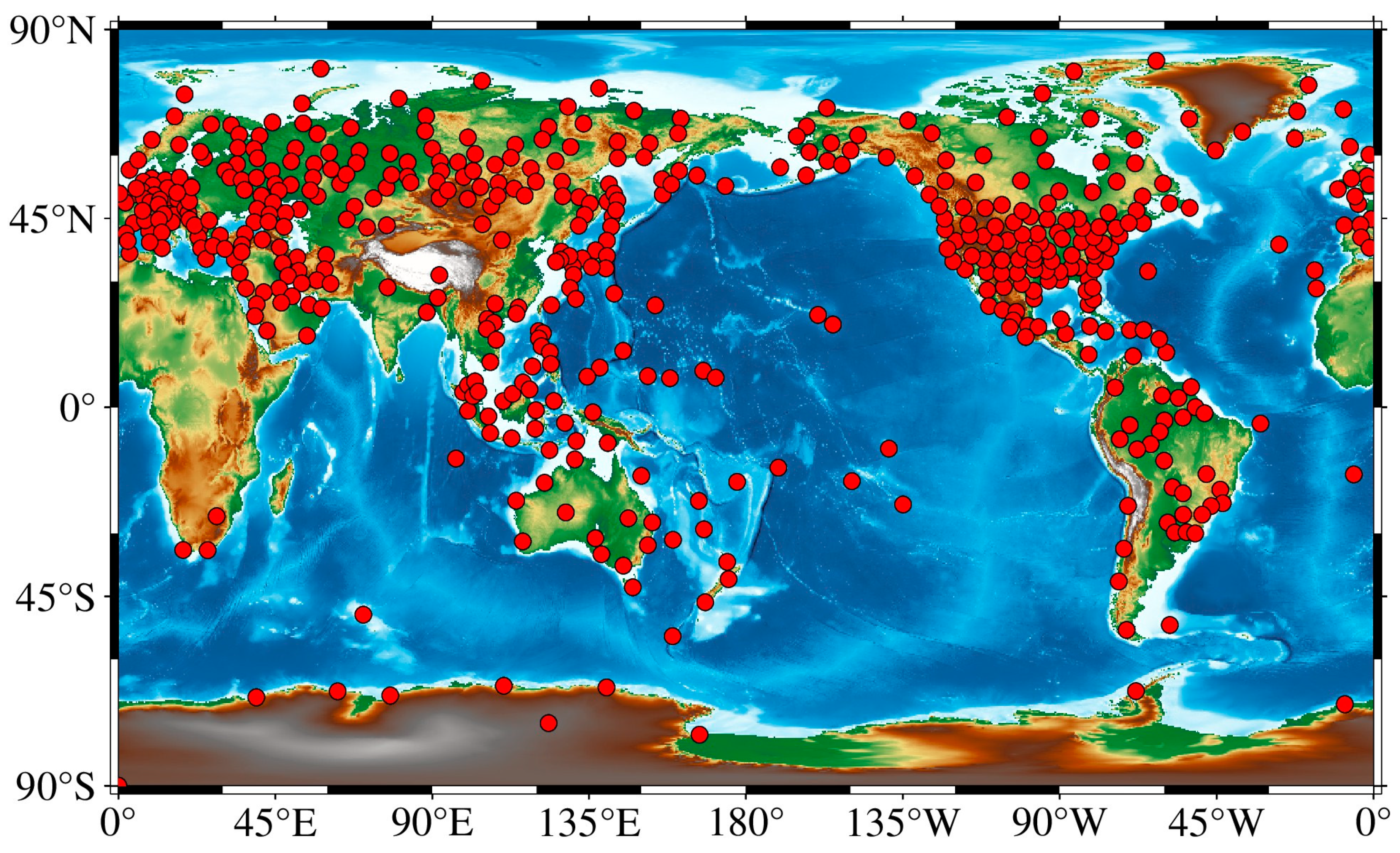
2.1. Radiosonde Data

Radiosonde sites collect stratified data on meteorological parameters such as pressure, temperature, and relative humidity from the surface to approximately 30 km above the surface. Radiosonde data are typically utilized as reference values for modeling validation [36,37,38,39,40]. ZWD is defined as the integral of the wet refractive index along the vertical profile above the radiosonde site and can be calculated using temperature and water vapor pressure integrals as follows [10,16]:

$$ZWD={10}^{-6}{\displaystyle \int N_w}dh={10}^{-6}{\displaystyle \int ({k^{\prime }}_2\frac{e}{T}+k_3\frac{e}{T}) }dh,$$

(1)

where $N_w$ denotes the wet refractive index, $e$ denotes water vapor pressure (hPa), $T$ denotes temperature (K), ${k^{\prime }}_2=16.52 K/hPa$, and $k_3=377,600 K^2/hPa$. To maintain uniformity in the elevation system, the geopotential heights provided by the radiosonde are converted into geodesic heights required by VMF3-FC. This is achieved by converting the geopotential heights to positive heights by using Equation (2) and then converting the positive heights to geodetic heights by using the Earth Gravitational Model 1996 (EGM96). More details regarding EGM96 can be found in the literature; see Lemoine et al. [41].

$$H_O(H_G,\phi )=\frac{R(\phi )\times Y_{45}\times H_G}{Y_s(\phi )\times R(\phi )-Y_{45}\times H_G},$$

(2)

where $H_O$ is the positive height, $Y_s(\phi )$ denotes the normal gravity value of the rotating ellipsoid surface, $R(\phi )$ denotes the effective radius of the earth at latitude $\phi$, and $Y_{45}$ denotes the normal gravity of the ellipsoid surface at a latitude of 45°, which is taken to be the value of $9.80665 m/s^2$ in this study. The equations for $Y_s(\phi )$ and $R(\phi )$ are as follows:

$$Y_s(\phi )=9.780358\times {[\frac{1+0.00193185\times \sin {\phi }^2}{1-0.00669435\times \sin {\phi }^2}]}^{0.5},$$

(3)

$$R(\phi )=\frac{6378.137}{1.006803-0.006706\times \sin {\phi }^2}.$$

(4)

We collected meteorological data from 492 radiosonde sites globally at two times per day (0:00 and 12:00 UTC) for 2019–2022 to obtain ZWD. The selection criteria were as follows: (1) Collection of radiosonde sites with data for 2019–2022. (2) Quality control. The period model based on the interquartile range (IQR) [42] (the specific formula refers to Zhao et al. [43]) was introduced to eliminate wide variations in the ZWD time series at each site. (3) Exclusion of sites with a lot of missing data after quality control. The distribution of the filtered radiosonde sites is shown in Figure 1. The observation data from 492 radiosonde sites from 2019–2021 were used for modeling, and observation data in 2022 were used for model accuracy validation.

2.2. VMF3-FC Data

The VMF data server provides reanalysis products (VMF-EI), operation products (VMF-OP), and forecast products (VMF-FC). VMF-FC can be used for real-time GNSS positioning and ZTD estimation. VMF3 is the latest version, and VMF3-FC provides two types of VMF forecast data based on the ECMWF 24-h NWP model: grid-based data and data from specific sites. In this study, only the grid-based VMF3-FC forecast products were calibrated.

The grid-based VMF3-FC is available in two versions with horizontal resolutions of 1° × 1° and 5° × 5°. They can derive the priori ZHD and ZWD and the coefficients of their corresponding mapping functions for four times (0:00, 6:00, 12:00, and 18:00 UTC) for each grid the following day. When it is necessary to obtain the ZWD at a specific, on the time scale, the values from two neighboring numerical weather model epochs are linearly interpolated to the desired moment. On the horizontal scale, bilinear interpolation is performed. On the vertical scale, specific formulas proposed by Kouba [44] are employed to extrapolate the ZWD from the respective heights of the grid points to that of the desired location. Yang et al. [45] revealed that the accuracy of the 1° × 1° VMF3 model in obtaining the ZWD is superior to that of the 1° × 1° VMF3 model by using the hourly values of the ERA5 and IGS data as references. Therefore, we used the ZWD derived from 1° × 1° VMF3-FC in this study. Furthermore, the VMF data server provides a code for VMF3-FC interpolation to obtain the ZHD and ZWD and their corresponding mapping function coefficients at specific points. This code was employed to interpolate and obtain the 2019–2022 VMF3-FC ZWD for the 492 radiosonde sites. The Software of MATLAB2019b is applied to run the code and the main parameter settings and sources of the code are summarized in

Table 1. Information and parameterization of the VMF3-FC for obtaining ZWDs.

Term	Information
Production	VMF3-FC
Horizontal resolution	indir_VMF3_grid with 1° × 1°
Satellite altitude angle	10°
Score	vmf3_grid.m https://vmf.geo.tuwien.ac.at/codes/ (accessed on 2 April 2023)
Gridded VMF3 files	orography_ell_1x1 http://vmf.geo.tuwien.ac.at/trop_products/GRID/ (accessed on 2 April 2023)
Input parameters	modified Julian date; ellipsoidal latitude (rad); ellipsoidal longitude (rad); ellipsoidal height (m); zenith distance (rad); grid resolution (°) (1)
Output parameters	zenith wet delay (m)

.

2.3. Comparative Model

The GPT3 model [23] is the latest version of the GPT serial model. The GPT3 model calculates meteorological parameters such as temperature and water vapor pressure based on a grid-format meteorological data storage file by inputting the modified Julian day, latitude, longitude, and geodetic height. The target meteorological parameters for a specific site and epoch can be determined by interpolation [23]. Then, the site-specific ZWD can be calculated by using Equation (1). The equations of the GPT3 model for calculating meteorological parameters for the grid points are as follows:

$$r\left(t\right)=A0+A1\cos \left(\frac{\mathrm{doy}}{365.25}2\pi \right)+B1\sin \left(\frac{doy}{365.25}2\pi \right)+A2\cos \left(\frac{doy}{365.25}4\pi \right)+B2\sin \left(\frac{doy}{365.25}4\pi \right),$$

(5)

where $r(t)$ is the meteorological parameter, $doy$ is the day of year, $A0$ is the mean value, and $A1$, $B1$, $A2$, and $B2$ are the annual and semiannual periodic amplitudes, respectively. The GPT3 model provides two versions with horizontal resolutions of 1° × 1° and 5° × 5°. The GPT3 model with a horizontal resolution of 1° × 1° was used to obtain the ZWD at 492 radiosonde sites in 2022 for the calibrated model validation.

3. Methodology

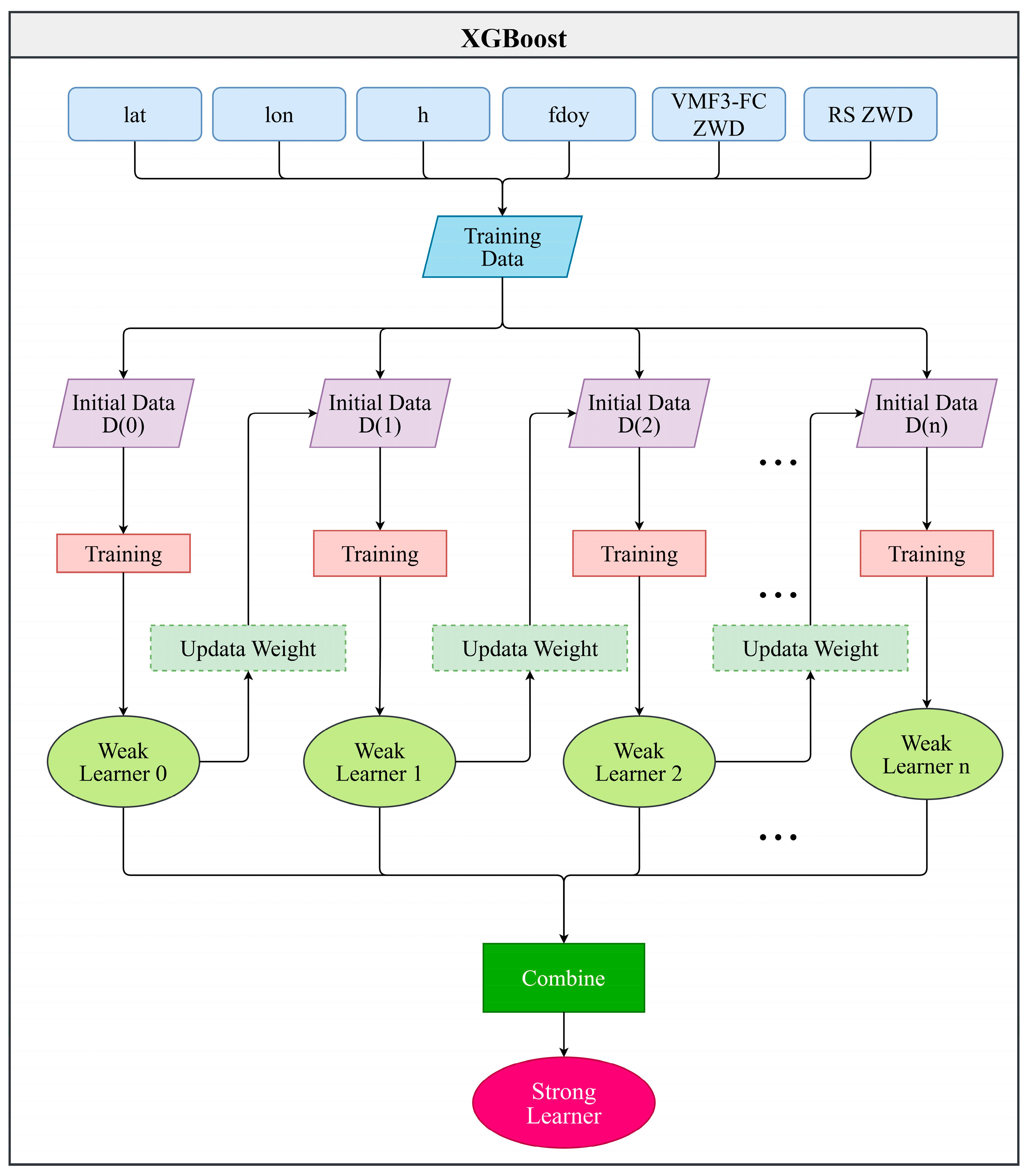
3.1. Construction of Calibrated Model

XGBoost was developed by Chen and Guestrin [46] based on gradient boosting decision trees [47]. XGBoost belongs to an ensemble algorithm. The ensemble algorithm trains several weak learners and then combines them to form a strong learner. Thus, the model constructed based on it has better predictive performance and robustness. Furthermore, XGBoost belongs to the boosting algorithm in the ensemble algorithm, which can effectively reduce the bias. In the case of XGBoost, the weak learner is typically a tree model. XGBoost forecasting involves continuously adding a tree model, dividing the growth tree by its characteristics, and then fitting the residuals of the previous forecast. The final prediction is the sum of the predictions obtained from each tree and can be expressed as follows:

$${\widehat{y}}_i={\displaystyle \sum _{k=1}^K{f}_k(x_i)}={\widehat{y}}_i^{<k-1>}+f_k(x_i),$$

(6)

where $x_i$ is the i-th sample, the total number of samples is $n$, $k$ is the k-th tree, ${\widehat{y}}_i$ is the predicted value of the i-th sample $x_i$, and $f_k$ is the independent tree (i.e., the k-th weak learner). The objective function of the k-th weak learner is the superposition of the loss function $l$ and the penalty function $\Omega$ and can be expressed as follows:

$$Obj={\displaystyle \sum _{i=1}^{n}l(\widehat{y_i},y_i)}+{\displaystyle \sum _{k=1}^K\Omega (f_k)}.$$

(7)

From Equations (6) and (7), the objective function obtained by training the k-th tree is obtained as follows:

$$Ob{j}_k={\displaystyle \sum _{i=1}^{n}l(y_i,{\widehat{y}}_i^{<k-1>}+f_k(x_i))}+\Omega (f_k).$$

(8)

Second-order Taylor expansion and regularized term expansion are performed successively, and then the constant term is removed, yielding the observation function as follows:

$$Ob{j}_k={\displaystyle \sum _{i=1}^n[g_i\cdot f_k(x_i)+\frac{1}{2}{h}_i\cdot f_k^2(x_i)]}+\Omega (f_k),$$

(9)

where $g_i$ and $h_i$ are the respective first- and second-order derivatives of ${\widehat{y}}_i^{<k-1>}$.

The complexity of a tree is defined in terms of the number of leaf nodes $t$ and the $l_2$ paradigm of the leaf node weight vector. Therefore, the penalty formula of the model is as follows:

$$\Omega (f_k)=\gamma \mathrm{t}+\frac{1}{2}\lambda {\displaystyle \sum _{j=1}^t{\omega }_{j=1}^2}.$$

(10)

Combining Equations (8) and (10) and grouping by leaf nodes yields the objective function as follows:

$$Ob{j}_k={\displaystyle \sum _{j=1}^t\left[G_j{\omega }_j+\frac{1}{2}(H_j+\lambda ){\omega }_j^2\right]}+\gamma t,$$

(11)

where $G_j$ and $H_j$ are the respective cumulative sum of the first- and second-order partial derivatives of the samples contained in the leaf node $j$; both are constants. The objective equations for each leaf node of the XGBoost objective function are independent, and for a tree, the objective function is computed once per split. When the information obtained from a split exceeds a predetermined threshold, the tree stops splitting, and the structure score of the tree becomes the final objective function. In this instance, the equation for each leaf node reaches the maximum value, the objective function reaches the maximum value, and the weight of each leaf node and the optimal objective value achieved can be expressed as follows:

$${\omega }_j^{\ast }=\frac{G_j}{H_j+\lambda },$$

(12)

$$Ob{j}^{\ast }=-\frac{1}{2}{\displaystyle \sum _{j=1}^t\frac{G_j^2}{H_j+\lambda }}+\gamma t.$$

(13)

The ZWD exhibits considerable temporal and spatial variations [48,49]. Therefore, we used latitude (lat), longitude (lon), height (h), floating day of year (fdoy), and VMF3-FC ZWD as the input and radiosonde ZWD (RS ZWD) as the output to construct a training sample and developed a calibrated model of VMF3-FC ZWD by using XGBoost. The structure of XGBoost is illustrated in Figure 2. Notably, in this paper, the interpolated ZWD is trained directly and the location information is used as the model factor, so the XZWD model can absorb the errors arising from the horizontal (latitude and longitude) interpolation and elevation correction. When the XZWD model is applied, the location information, epoch information, and VMF3-FC ZWD of the target point are first collected. Then, they are input into the XZWD model to achieve the ZWD of the target point with higher accuracy.

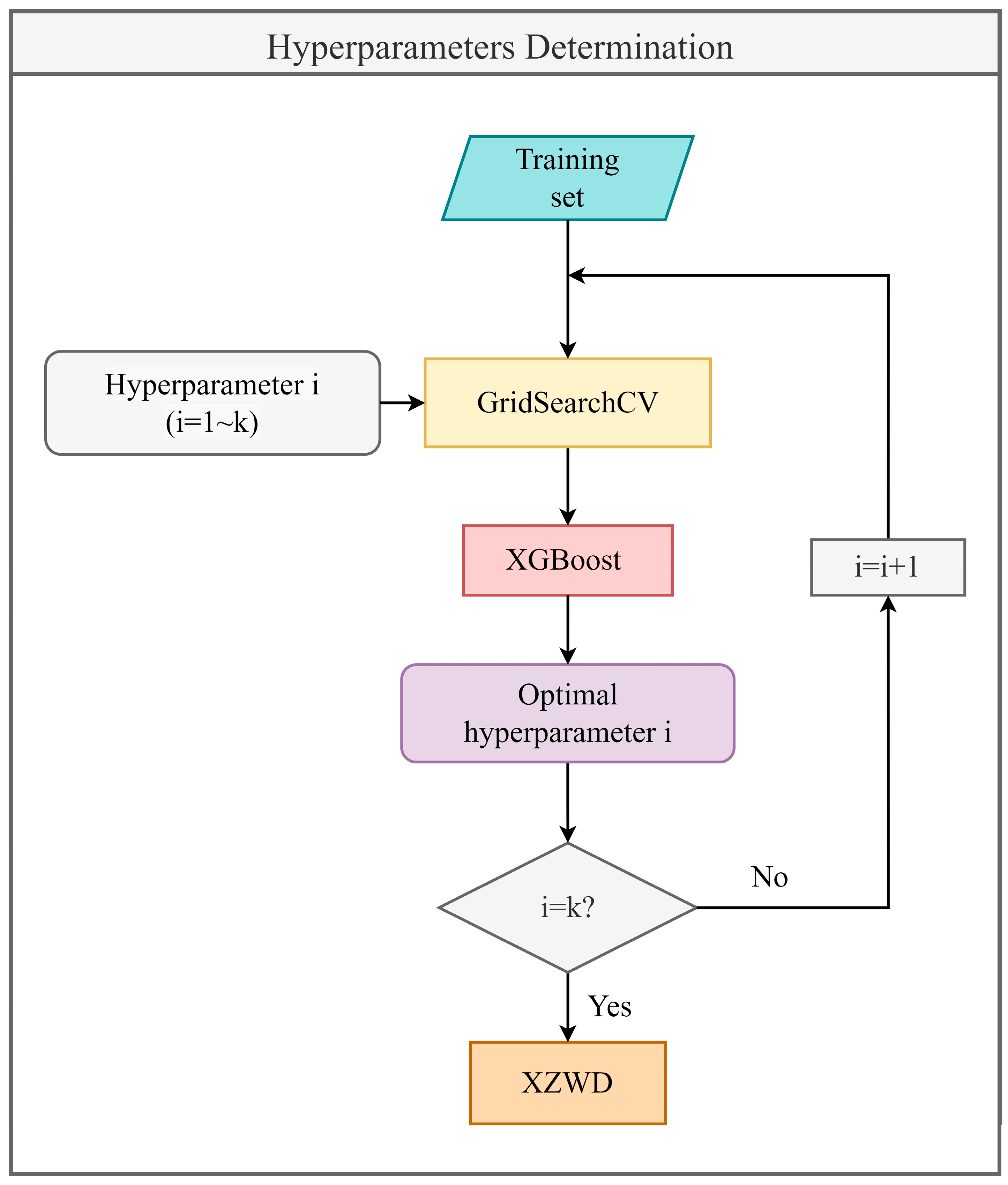
3.2. Hyperparameter Determination

The hyperparameters of the XGBoost algorithm are defined as values or weights that can determine the learning properties of the algorithm [50]. We determined these hyperparameters by using the GridSearchCV (sklearn.model_selection.GridSearchCV (https://scikit-learn.org/stable/modules/generated/sklearn.model_selection.GridSearchCV.html#sklearn.model_selection.GridSearchCV, accessed on 2 February 2023)) method available in Scikit-learn [51]. We provide a set of tried values for the hyperparameters, and the GridSearchCV is trained on the different tried values. Next, GridSearchCV yields the evaluation index scores for all combinations of hyperparameters through cross-validation and finally outputs the best score and the corresponding best hyperparameter values. Only one or two hyperparameters are determined at a time, and the other hyperparameters are assigned an initial value. After the optimal hyperparameters are determined, their initial values are replaced with the obtained optimal hyperparameter values. This process is repeated using GridSearchCV to continue determining the rest of the hyperparameters. The flowchart for hyperparameter determination of the XZWD model is shown in Figure 3. The hyperparameters that need to be determined and their order, initial values, the tried values, the best score, and the corresponding best hyperparameter values after 10-fold cross-validation are displayed in

Table 2. Hyperparameter settings and the results of hyperparameter determination.

Order	Hyperparameters	Initial Value	Tried Value	Best Score	Best Hyperparameters
1	n_estimators	500	[100, 200, 300, 400, 500]	0.97	300
2	max_depth	5	[3, 4, 5, 6, 7, 8, 9, 10]	0.97	7
2	min_child_weight	1	[1, 2, 3, 4, 5, 6]	0.97	5
3	gamma	0	[0, 0.1, 0.2, 0.3, 0.4, 0.5]	0.97	0
4	subsample	0.8	[0.6, 0.7,0.8, 0.9]	0.97	0.9
4	colsample_bytree	0.8	[0.6, 0.7,0.8, 0.9]	0.97	0.8
5	learning_rate	0.1	[0.01, 0.05, 0.1, 0.2, 0.3, 0.4, 0.5]	0.97	0.2
6	n_estimators	500	[100, 200, 300, 400, 500]	0.97	300

. The optimal ZWD calibrated model is constructed based on the optimal values of all hyperparameters being determined. Note that when using this model to estimate ZWD, we only need to input the 3D coordinates of the user site, fdoy, and VMF3-FC ZWD. The Software of Python 3.10 is employed for hyperparameter determination and the XZWD model construction.

3.3. Model Validation and Evaluation

Two statistical metrics, bias and RMSE, were introduced as criteria to assess model performance:

$$Bias=\frac{1}{N}{\displaystyle \sum _{i=1}^N(ZW{D}_i-ZW{D}_i^R)},$$

(14)

$$RMSE=\sqrt{\frac{1}{N}{\displaystyle \sum _{i=1}^N{(ZW{D}_i-ZW{D}_i^R)}^2}}.$$

(15)

where $ZW{D}_i$ denotes the ZWD derived from models, $ZW{D}_i^R$ denotes the reference ZWD, and $N$ is the total number of ZWDs.

4. Assessment of the Calibrated Model

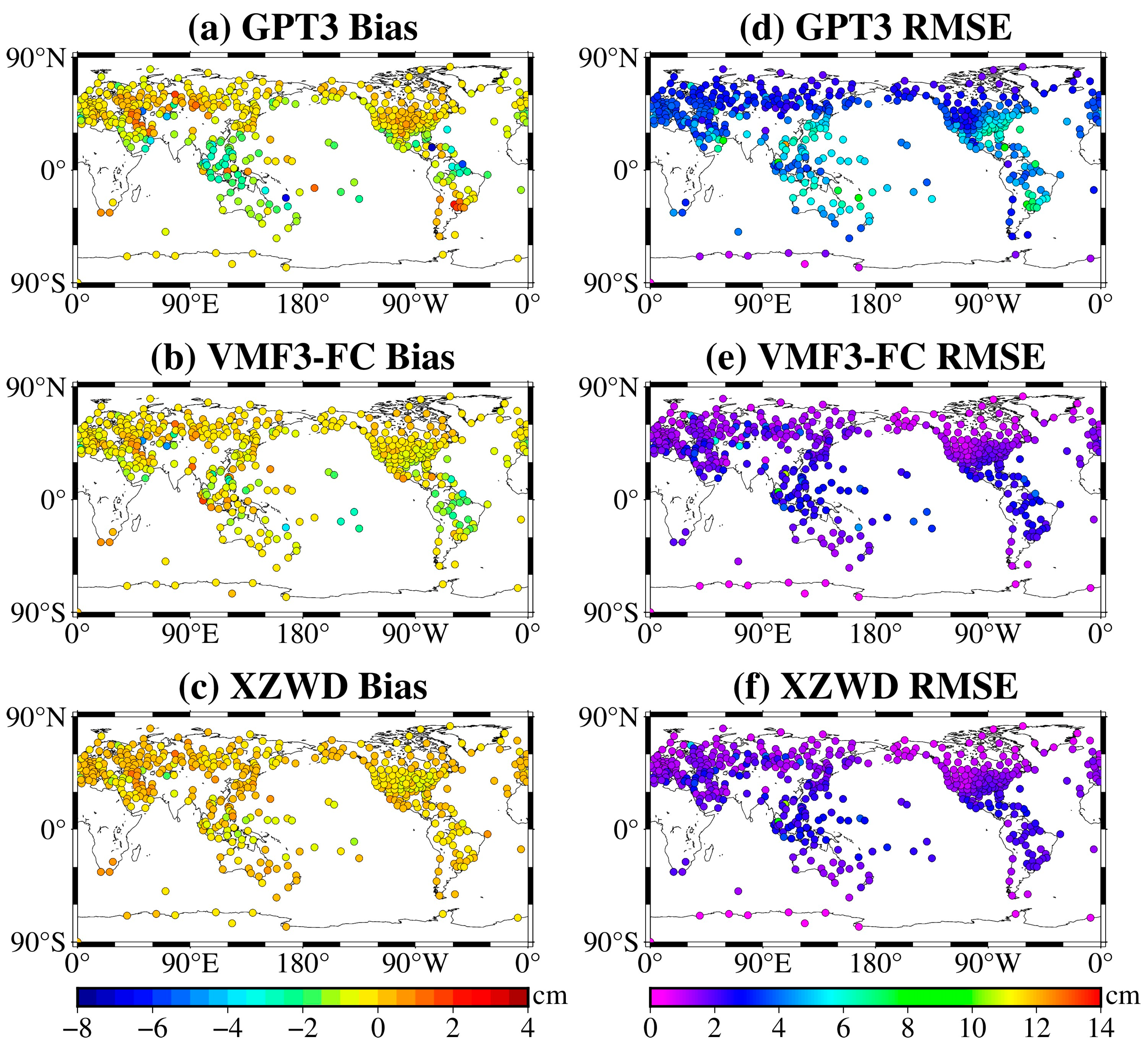
4.1. Global Accuracies

The XZWD, VMF3-FC, and GPT3-derived ZWD were compared with RS ZWD at 492 sites in 2022 for validation. The results are presented in

Table 3. Mean bias and RMSE of the ZWD for the three models.

	GPT3	VMF3-FC	XZWD
Bias (cm)	−0.56	−0.41	−0.03
	[−7.31, 2.20]	[−4.89, 1.55]	[−1.61 1.05]
RMSE (cm)	3.99	1.75	1.64
	[0.21, 12.24]	[0.19, 10.68]	[0.12, 10.44]

, and the values within square brackets are the maximum and minimum. The bias and RMSE of the GPT3 model are −0.56 and 3.99 cm. The VMF3-FC exhibits superior ZWD accuracy compared to the GPT3 model, with a bias of −0.41 cm and an RMSE of 1.75 cm. The XZWD model yields a bias of −0.03 cm and an RMSE of 1.64 cm, an improvement of 92.7% and 6.3%, respectively, compared to VMF3-FC. The XZWD model exhibits better global ZWD accuracy than both VMF3-FC and the GPT3 model. In addition, the bias and RMSE of the XZWD model vary from −1.61 to 1.05 cm and from 0.12 to 10.44 cm, respectively. In contrast, the bias and RMSE of VMF3-FC vary from −4.89 to 1.55 cm and from 0.19 to 10.68 cm, respectively. These results illustrate the superior stability of the accuracy of the XZWD model in comparison to VMF3-FC. To further evaluate the calibration effect of the XZWD model, the accuracies of the GPT3, VMF3-FC, and XZWD models at each site are shown in Figure 4. The biases of the GPT3 model and VMF3-FC exhibit geographical variations, with a positive bias in the mid- to high latitudes and a negative bias near the equator. The XZWD model effectively reduces the negative bias at the equator and balances the bias distribution. Latitudinal variation is also observed in the RMSEs of the GPT3, VMF3-FC, and XZWD models, with superior RMSEs in mid- to high latitudes compared to low latitudes. Furthermore, the RMSEs of the VMF3-FC and XZWD models remain within 4 cm at most sites, which is better than that of the GPT3 model. In addition, compared with VMF3-FC, the XZWD model greatly reduces larger RMSE anomalies (up to 5.0–10.0 cm) in western Asia and the Atlantic Equatorial Annex. In summary, the XZWD model exhibits fewer uncertainties than VMF3-FC and the GPT3 model.

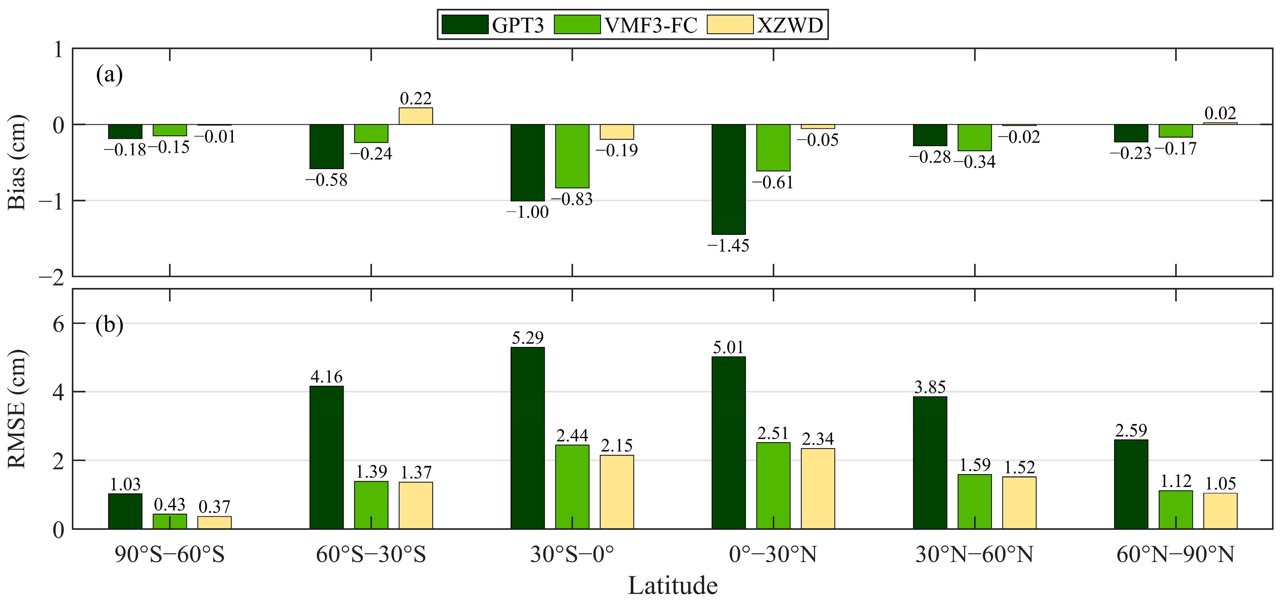
4.2. Accuracies in Different Latitude Belts

As seen from the results in Section 4.1, model accuracy varies with the latitude. To study the variations in the ZWD accuracy of the GPT3, VMF-FC, and XZWD models with latitude, first, we divided the area into six latitude bands with 30° intervals. Next, we calculated the mean bias and RMSE for each latitude band based on the sites located within the band. As can be seen from the bias and RMSE variations for the three models in the six latitude bands presented in Figure 5, the absolute values of bias and RMSE for all three models gradually decrease from the equatorial areas to the polar areas. The accuracy is poorer around the equatorial regions because water vapor varies greatly spatiotemporally in the equatorial region, making capturing and reproducing the ZWD challenging. The VMF3-FC ZWD exhibits smaller bias and RMSE compared to the GPT3 model in most latitude bands. However, in the 30° N–60° N latitudinal range, the VMF3-FC bias is −0.34 cm, a more significant deviation from 0 cm compared with that of the bias of the GPT3 model (−0.28 cm). This further indicates the uneven and unstable nature of VMF3-FC ZWD accuracy, thus necessitating calibration. In contrast, the XZWD model exhibits lower bias and RMSE values compared to the GPT3 model and VMF3-FC in all latitude bands. Compared to the GPT3 model and VMF3-FC, improvements of 94.4%/93.3%, 62.1%/8.3%, 81.0%/77.1%, 96.6/57.9%, 92.9/94.1%, and 91.3%/88.2% are observed in the biases of the XZWD model in the six latitude bands, respectively, and the RMSEs of the XZWD model decrease by 0.66/0.06, 2.79/0.02, 3.14/0.29, 2.67/0.17, 2.33/0.07, and 1.54/0.07 cm, respectively. Overall, the accuracy of the XZWD model is less affected by latitudinal variations; thus, indicating that it can provide a more accurate estimation of ZWD.

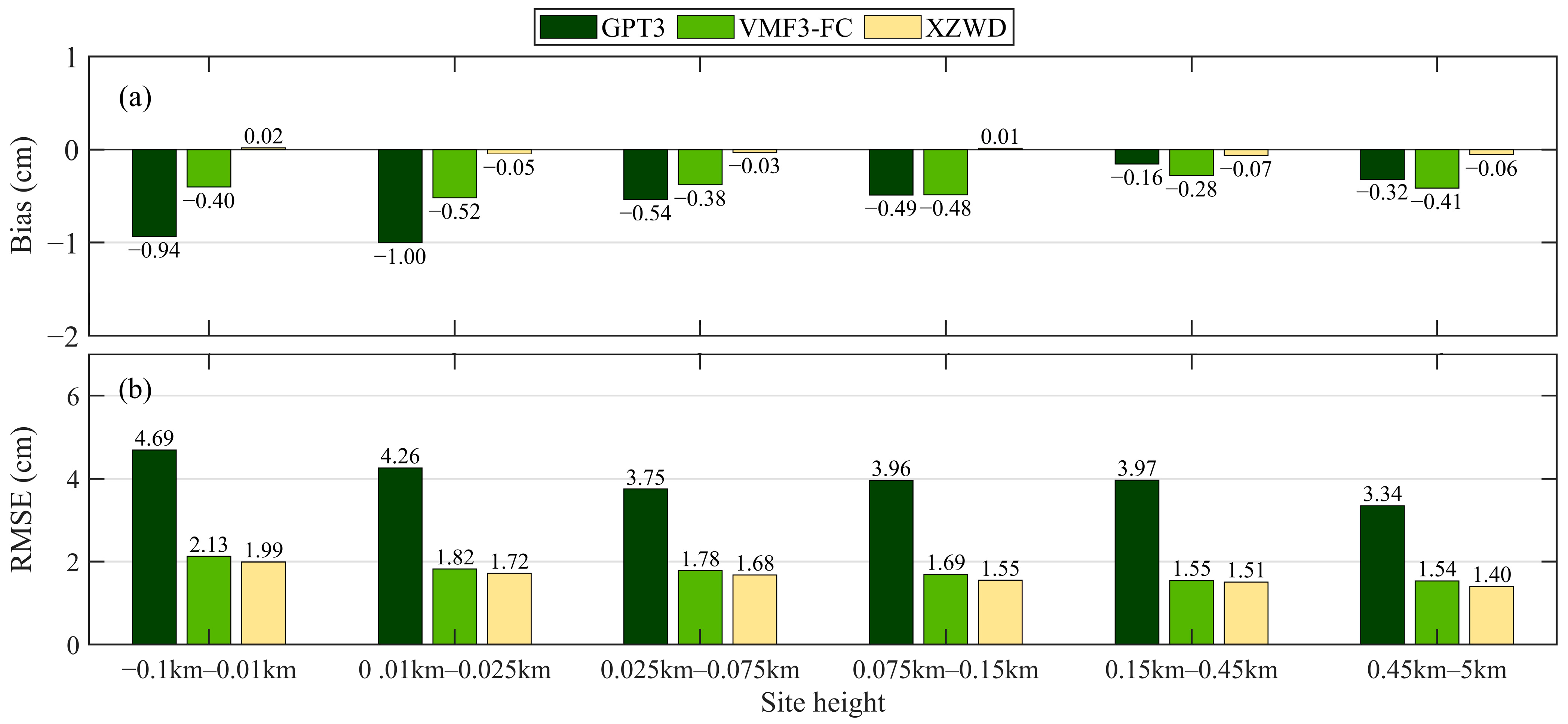
4.3. Accuracies in Different Height Ranges

ZWD accuracy is greatly affected by height variations [1,52,53]. Therefore, we divided the height range (−0.1–5 km) of the 492 sites into six height bands: −0.10–0.01 km, 0.01–0.025 km, 0.025–0.075 km, 0.075–0.15 km, 0.15–0.45 km, and 0.45–5.00 km. The number of sites within the six height bands and the bias and RMSE of the GPT3, VMF3-FC, and XZWD models within each height band are presented in

Table 4. Number of sites and ZWD accuracy for the three models in different height ranges.

Site Height (km)	Number	Bias (cm)			RMSE (cm)
		GPT3	VMF3-FC	XZWD	GPT3	VMF3-FC	XZWD
−0.10–0.010	85	−0.94	−0.40	0.02	4.69	2.13	1.99
0.010–0.025	72	−1.00	−0.52	−0.05	4.26	1.82	1.72
0.025–0.075	83	−0.54	−0.38	−0.03	3.75	1.78	1.68
0.075–0.150	84	−0.49	−0.48	0.01	3.96	1.69	1.55
0.150–0.450	85	−0.16	−0.28	−0.07	3.97	1.55	1.51
0.450–5.00	83	−0.32	−0.41	−0.06	3.34	1.54	1.40

. The GPT3 model and VMF3-FC yield negative biases, and the absolute values of bias vary from 0 to 1 cm. In contrast, the absolute values of bias of the XZWD model are within 0.1 cm. Compared with the GPT3 model and VMF3-FC, the bias of the XZWD model is lower. The ZWD of the XZWD model is in better agreement with the RS ZWD. The RMSE of the GPT3 model is greater than 3 cm in all six height bands, and the RMSE of VMF3-FC is smaller than 3 cm (1.5–2.2 cm). The RMSE of the XZWD model is smaller than 2 cm (1.4–2.0 cm), indicating its stable accuracy. Moreover, in each height band, the RMSE of the XZWD model is lower than that of VMF3-FC. To more graphically access the calibration effect of the XZWD model in different height belts, the ZWD accuracy of the three models in the six height bands is illustrated in Figure 6. The absolute value of bias of the three models varies greatly in the –0.1–0.15 km band and slightly in the 0.15–5 km band. The VMF3-FC exhibits a larger bias than the GPT3 model in the height range of 0.15–5 km, which indicates that VMF3-FC has a larger bias at greater heights. In contrast, the bias of the XZWD model is better than that of the GPT3 model and VMF3-FC in all height bands. The RMSE of the GPT3 model is larger than that of the VMF3-FC and XZWD models in most height bands. Furthermore, the RMSE of the XZWD model is better than that of VMF3-FC in all height bands, with a reduction of 0.14, 0.10, 0.10, 0.14, 0.04, and 0.14 cm, respectively, in the six height bands. The XZWD model exhibits better accuracy and stability than the GPT3 model and VMF3-FC at different heights.

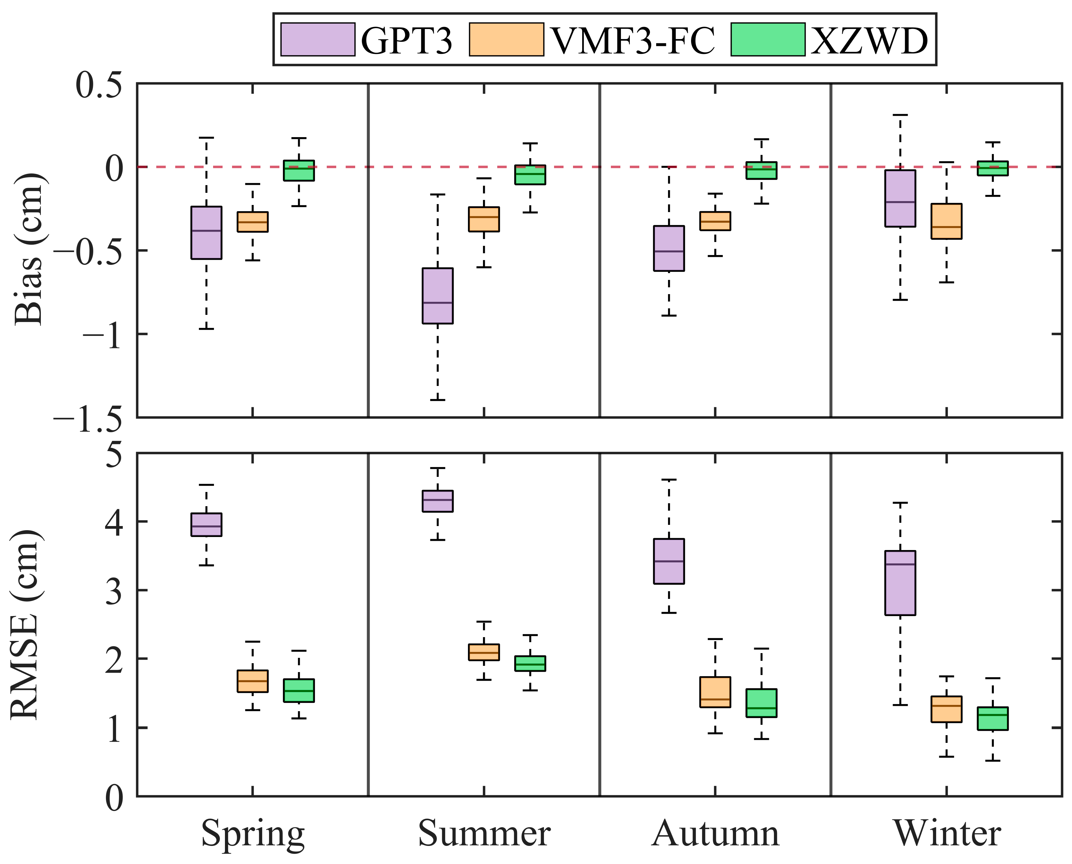
4.4. Accuracies in Different Seasons

The ZWD variations are correlated with seasons [48,49,54]. We calculated the bias and RMSE of the GPT3, VMF3-FC, and XZWD models in different seasons; the results are displayed in

Table 5. Mean bias and RMSE of ZWD for the three models in different seasons.

	Bias (cm)			RMSE (cm)
	GPT3	VMF3-FC	XZWD	GPT3	VMF3-FC	XZWD
Spring	−0.40	−0.33	−0.02	3.94	1.70	1.57
Summer	−0.77	−0.32	−0.05	4.33	2.17	2.01
Autumn	−0.48	−0.33	−0.02	3.44	1.53	1.39
Winter	−0.21	−0.33	−0.01	3.12	1.31	1.19

. In this work, Spring is March to May; Summer is June to August; Autumn is September to November; Winter is December to February. The table shows that the maximum values of the bias and RMSE of the GPT3 model appear in summer, i.e., −0.40 and 4.33 cm, respectively. The minimum values appear in winter, which are −0.21 and 3.12 cm, respectively. Compared with the GPT3 model, the seasonal difference in bias of VMF3-FC is smaller, with an average of about −0.33 cm. The maximum RMSE of VMF3-FC is 2.17 cm in summer, and the minimum is 1.31 cm in winter. Compared with the GPT3 model and VMF3-FC, the bias correction of the XZWD model is significant, with an average bias of −0.03 cm. The maximum RMSE in summer is reduced to 2.01 cm, and the minimum RMSE in winter is reduced to 1.19 cm. The boxplot of the bias and RMSE of ZWD from the three models in different seasons is shown in Figure 7. The biases of VMF3-FC and the XZWD model exhibit less variability than that of the GPT3 model. The bias of the XZWD model is more concentrated than the VMF3-FC bias, and the median bias of the XZWD model is closer to 0 cm than that of VMF3-FC. The RMSEs of the GPT3, VMF3-FC, and XZWD models are larger in summer and smaller in winter. In addition, the RMSE is relatively dispersed in autumn and winter and relatively concentrated in spring and summer. The RMSEs of VMF3-FC and the XZWD model are less than 3 cm, which is better than that of the GPT3 model. Furthermore, compared with the RMSE from VMF3-FC, the RMSE of the XZWD model improves in all seasons, and the XZWD model yields higher ZWD accuracy. Overall, the XZWD model reduces specific seasonal differences in ZWD accuracy.

5. Discussion

In this work, a globally calibrated model called XZWD for VMF3-FC ZWD based on the XGBoost algorithm was developed.

We investigated the XGBoost algorithms and then chose latitude, longitude, height, floating day of year, and VMF3-FC ZWD as the input and radiosonde ZWD as the output for modeling to better map the spatial and temporal variations in the relationship between the measured ZWD and VMF3-FC ZWD. Furthermore, the interpolated VMF3-FC ZWD was directly selected for training to ensure the simplicity and practicability of the model as well as to minimize the errors resulting from horizontal (latitude and longitude) and spatial interpolation. Details of the operation can be found in Section 3.

From Table 3 and Figure 4, the overall accuracy of the XZWD model is found to be significantly better than the internationally recognized classical empirical model GPT3 and the original VMF3-FC. From Figure 5 and Figure 6, and Table 4, it is found that the XZWD model, compared to the GPT3 model and VMF3-FC, reduces the differences in ZWD accuracy in terms of latitude and site heights, and especially at low latitudes and high heights, XZWD shows better accuracy. The results from Table 5 and Figure 7 reveal that on the time scale, the XZWD model reduces the influence of ZWD by season. The XZWD model has a more stable and accurate ZWD estimation.

6. Conclusions

ZWD derived from NWP is commonly employed in GNSS positioning and PWV inversion. As such, its accuracy is crucial. In this study, we developed a globally calibrated model called XZWD for VMF3-FC ZWD based on the XGBoost algorithm by using latitude, longitude, height, floating day of year, and VMF3-FC ZWD as the input and RS ZWD as the output. In addition, we validated the calibrated model by using the radiosonde data not involved in modeling. The results revealed that the bias and RMSE of the XZWD model are −0.03 and 1.64 cm, respectively, which are better than those of the GPT3 model and VMF3-FC, with improvements of 94.64%/92.68% and 58.90%/6.29%, respectively. Furthermore, we performed comprehensive comparisons between the XZWD model and two compaction models for different latitudes, heights, and seasons. The GPT3 model and VMF3-FC exhibit poor accuracy in low-latitude and high-height areas, whereas the XZWD model exhibits excellent and stable accuracy in all latitude bands and height bands. The XZWD model yields lower seasonal variations and discretization of the ZWD accuracy compared to the GPT3 model and VMF3-FC. In addition, the XZWD model yields superior accuracy and stability compared to the GPT3 model and VMF3-FC, thereby effectively calibrating the VMF3-FC ZWD. Therefore, the XZWD model can be employed for VMF3-FC ZWD calibration and is suitable for real-time GNSS positioning and PWV inversion.

References

1. Yang, F.; Guo, J.; Meng, X.; Li, J.; Zou, J.; Xu, Y. Establishment and Assessment of a Zenith Wet Delay (ZWD) Augmentation Model. GPS Solut. 2021, 25, 148. [Google Scholar] [CrossRef]
2. Xia, P.; Tong, M.; Ye, S.; Qian, J.; Fangxin, H. Establishing a High-Precision Real-Time ZTD Model of China with GPS and ERA5 Historical Data and Its Application in PPP. GPS Solut. 2022, 27, 2. [Google Scholar] [CrossRef]
3. Zhang, H.; Yao, Y.; Hu, M.; Xu, C.; Su, X.; Che, D.; Peng, W. A Tropospheric Zenith Delay Forecasting Model Based on a Long Short-Term Memory Neural Network and Its Impact on Precise Point Positioning. Remote Sens. 2022, 14, 5921. [Google Scholar] [CrossRef]
4. Li, J.; Zhang, Q.; Liu, L.; Yao, Y.; Huang, L.; Chen, F.; Zhou, L.; Zhang, B. A Refined Zenith Tropospheric Delay Model for Mainland China Based on the Global Pressure and Temperature 3 (GPT3) Model and Random Forest. GPS Solut. 2023, 27, 172. [Google Scholar] [CrossRef]
5. Zhao, Q.; Su, J.; Xu, C.; Yao, Y.; Zhang, X.; Wu, J. High-Precision ZTD Model of Altitude-Related Correction. IEEE J. Sel. Top. Appl. Earth Obs. Remote Sens. 2023, 16, 609–621. [Google Scholar] [CrossRef]
6. Li, H.; Zhu, G.; Kang, Q.; Huang, L.; Wang, H. A Global Zenith Tropospheric Delay Model with ERA5 and GNSS-Based ZTD Difference Correction. GPS Solut. 2023, 27, 154. [Google Scholar] [CrossRef]
7. Zhang, H.; Yuan, Y.; Li, W. An Analysis of Multisource Tropospheric Hydrostatic Delays and Their Implications for GPS/GLONASS PPP-Based Zenith Tropospheric Delay and Height Estimations. J. Geod. 2021, 95, 83. [Google Scholar] [CrossRef]
8. Zhang, H.; Yuan, Y.; Li, W. Real-Time Wide-Area Precise Tropospheric Corrections (WAPTCs) Jointly Using GNSS and NWP Forecasts for China. J. Geod. 2022, 96, 44. [Google Scholar] [CrossRef]
9. Li, L.; Xu, Y.; Yan, L.; Wang, S.; Liu, G.; Liu, F. A Regional NWP Tropospheric Delay Inversion Method Based on a General Regression Neural Network Model. Sensors 2020, 20, 3167. [Google Scholar] [CrossRef]
10. Davis, J.L.; Herring, T.A.; Shapiro, I.I.; Rogers, A.E.E.; Elgered, G. Geodesy by Radio Interferometry: Effects of Atmospheric Modeling Errors on Estimates of Baseline Length. Radio Sci. 1985, 20, 1593–1607. [Google Scholar] [CrossRef]
11. Ziv, S.Z.; Reuveni, Y. Flash Floods Prediction Using Precipitable Water Vapor Derived from GPS Tropospheric Path Delays over the Eastern Mediterranean. IEEE Trans. Geosci. Remote Sens. 2022, 60, 5804017. [Google Scholar] [CrossRef]
12. Wang, H.; Liu, Y.; Liu, Y.; Cao, Y.; Liang, H.; Hu, H.; Liang, J.; Tu, M. Assimilation of GNSS PWV with NCAR-RTFDDA to Improve Prediction of a Landfall Typhoon. Remote Sens. 2022, 14, 178. [Google Scholar] [CrossRef]
13. Guo, A.; Xu, Y.; Jiang, N.; Wu, Y.; Gao, Z.; Li, S.; Xu, T.; Bastos, L. Analyzing Correlations between GNSS Retrieved Precipitable Water Vapor and Land Surface Temperature after Earthquakes Occurrence. Sci. Total Environ. 2023, 872, 162225. [Google Scholar] [CrossRef] [PubMed]
14. Kawo, A.; Van Schaeybroeck, B.; Van Malderen, R.; Pottiaux, E. Precipitable Water Vapor in Regional Climate Models over Ethiopia: Model Evaluation and Climate Projections. Clim. Dyn. 2023, 1–21. [Google Scholar] [CrossRef]
15. Li, H.; Wang, X.; Choy, S.; Jiang, C.; Wu, S.; Zhang, J.; Qiu, C.; Zhou, K.; Li, L.; Fu, E.; et al. Detecting Heavy Rainfall Using Anomaly-Based Percentile Thresholds of Predictors Derived from GNSS-PWV. Atmos. Res. 2022, 265, 105912. [Google Scholar] [CrossRef]
16. Bevis, M.; Businger, S.; Herring, T.A.; Rocken, C.; Anthes, R.A.; Ware, R.H. GPS Meteorology: Remote Sensing of Atmospheric Water Vapor Using the Global Positioning System. J. Geophys. Res. 1992, 97, 15787. [Google Scholar] [CrossRef]
17. Graffigna, V.; Hernández-Pajares, M.; Azpilicueta, F.; Gende, M. Comprehensive Study on the Tropospheric Wet Delay and Horizontal Gradients during a Severe Weather Event. Remote Sens. 2022, 14, 888. [Google Scholar] [CrossRef]
18. Chen, B.; Liu, Z. A Comprehensive Evaluation and Analysis of the Performance of Multiple Tropospheric Models in China Region. IEEE Trans. Geosci. Remote Sens. 2016, 54, 663–678. [Google Scholar] [CrossRef]
19. Srivastava, A. Accuracy Assessment of Reanalysis Datasets for GPS-PWV Estimation Using Indian IGS Stations Observations. Geocarto Int. 2022, 37, 9644–9662. [Google Scholar] [CrossRef]
20. Boehm, J.; Heinkelmann, R.; Schuh, H. Short Note: A Global Model of Pressure and Temperature for Geodetic Applications. J. Geod. 2007, 81, 679–683. [Google Scholar] [CrossRef]
21. Lagler, K.; Schindelegger, M.; Böhm, J.; Krásná, H.; Nilsson, T. GPT2: Empirical Slant Delay Model for Radio Space Geodetic Techniques. Geophys. Res. Lett. 2013, 40, 1069–1073. [Google Scholar] [CrossRef]
22. Böhm, J.; Möller, G.; Schindelegger, M.; Pain, G.; Weber, R. Development of an Improved Empirical Model for Slant Delays in the Troposphere (GPT2w). GPS Solut. 2015, 19, 433–441. [Google Scholar] [CrossRef]
23. Landskron, D.; Böhm, J. VMF3/GPT3: Refined Discrete and Empirical Troposphere Mapping Functions. J. Geod. 2018, 92, 349–360. [Google Scholar] [CrossRef] [PubMed]
24. Collins, J.P.; Langley, R.B. A Tropospheric Delay Model for the User of the Wide Area Augmentation System; University of New Brunswick: Federiction, NB, Canada, 1997. [Google Scholar]
25. Leandro, R.F.; Langley, R.B.; Santos, M.C. UNB3m_pack: A Neutral Atmosphere Delay Package for Radiometric Space Techniques. GPS Solut. 2008, 12, 65–70. [Google Scholar] [CrossRef]
26. Yuan, Y.; Holden, L.; Kealy, A.; Choy, S.; Hordyniec, P. Assessment of Forecast Vienna Mapping Function 1 for Real-Time Tropospheric Delay Modeling in GNSS. J. Geod. 2019, 93, 1501–1514. [Google Scholar] [CrossRef]
27. Zhang, W.; Zhang, H.; Liang, H.; Lou, Y.; Cai, Y.; Cao, Y.; Zhou, Y.; Liu, W. On the Suitability of ERA5 in Hourly GPS Precipitable Water Vapor Retrieval over China. J. Geod. 2019, 93, 1897–1909. [Google Scholar] [CrossRef]
28. Sun, P.; Zhang, K.; Wu, S.; Wan, M.; Lin, Y. Retrieving Precipitable Water Vapor from Real-Time Precise Point Positioning Using VMF1/VMF3 Forecasting Products. Remote Sens. 2021, 13, 3245. [Google Scholar] [CrossRef]
29. Selbesoglu, M.O. Prediction of Tropospheric Wet Delay by an Artificial Neural Network Model Based on Meteorological and GNSS Data. Eng. Sci. Technol. Int. J. 2020, 23, 967–972. [Google Scholar] [CrossRef]
30. Ghaffari Razin, M.-R.; Voosoghi, B. Modeling of Precipitable Water Vapor from GPS Observations Using Machine Learning and Tomography Methods. Adv. Space Res. 2022, 69, 2671–2681. [Google Scholar] [CrossRef]
31. Zhu, M.; Yu, X.; Sun, W. A Coalescent Grid Model of Weighted Mean Temperature for China Region Based on Feedforward Neural Network Algorithm. GPS Solut. 2022, 26, 70. [Google Scholar] [CrossRef]
32. Zheng, Y.; Lu, C.; Wu, Z.; Liao, J.; Zhang, Y.; Wang, Q. Machine Learning-Based Model for Real-Time GNSS Precipitable Water Vapor Sensing. Geophys. Res. Lett. 2022, 49, e2021GL096408. [Google Scholar] [CrossRef]
33. Gu, Z.; Cao, M.; Wang, C.; Yu, N.; Qing, H. Research on Mining Maximum Subsidence Prediction Based on Genetic Algorithm Combined with XGBoost Model. Sustainability 2022, 14, 10421. [Google Scholar] [CrossRef]
34. Sridharan, M. Performance Augmentation Study on a Solar Flat Plate Water Collector System with Modified Absorber Flow Design and Its Performance Prediction Using the XGBoost Algorithm: A Machine Learning Approach. Iran. J. Sci. Technol. Trans. Mech. Eng. 2023, 1–12. [Google Scholar] [CrossRef]
35. Xu, B.; Tan, Y.; Sun, W.; Ma, T.; Liu, H.; Wang, D. Study on the Prediction of the Uniaxial Compressive Strength of Rock Based on the SSA-XGBoost Model. Sustainability 2023, 15, 5201. [Google Scholar] [CrossRef]
36. Aragón Paz, J.M.; Mendoza, L.P.O.; Fernández, L.I. Near-Real-Time GNSS Tropospheric IWV Monitoring System for South America. GPS Solut. 2023, 27, 93. [Google Scholar] [CrossRef]
37. Trzcina, E.; Rohm, W.; Smolak, K. Parameterisation of the GNSS Troposphere Tomography Domain with Optimisation of the Nodes’ Distribution. J. Geod. 2022, 97, 2. [Google Scholar] [CrossRef]
38. Zhang, H.; Yuan, Y.; Li, W.; Ou, J.; Li, Y.; Zhang, B. GPS PPP-Derived Precipitable Water Vapor Retrieval Based on Tm/Ps from Multiple Sources of Meteorological Data Sets in China: GPS-PWV Retrieval on Multiple Data Sets. J. Geophys. Res. Atmos. 2017, 122, 4165–4183. [Google Scholar] [CrossRef]
39. Huang, L.; Liu, W.; Mo, Z.; Zhang, H.; Li, J.; Chen, F.; Liu, L.; Jiang, W. A New Model for Vertical Adjustment of Precipitable Water Vapor with Consideration of the Time-Varying Lapse Rate. GPS Solut. 2023, 27, 170. [Google Scholar] [CrossRef]
40. Huang, L.; Zhu, G.; Peng, H.; Liu, L.; Ren, C.; Jiang, W. An Improved Global Grid Model for Calibrating Zenith Tropospheric Delay for GNSS Applications. GPS Solut. 2022, 27, 17. [Google Scholar] [CrossRef]
41. Lemoine, F.; Kenyon, S.C.; Factor, J.; Trimmer, R.; Pavlis, N.; Chinn, D.; Cox, C.; Klosko, S.; Luthcke, S.; Torrence, M.; et al. The Development of the Joint NASA GSFC and the National Imagery and Mapping Agency (NIMA) Geopotential Model EGM96; National Aeronautics and Space Administration, Goddard Space Flight Center: Greenbelt, MD, USA, 1998; Volume 206861.
42. Xie, W.; Huang, G.; Fu, W.; Shu, B.; Cui, B.; Li, M.; Yue, F. A Quality Control Method Based on Improved IQR for Estimating Multi-GNSS Real-Time Satellite Clock Offset. Measurement 2022, 201, 111695. [Google Scholar] [CrossRef]
43. Zhao, Q.; Ma, X.; Yao, W.; Liu, Y.; Yao, Y. A Drought Monitoring Method Based on Precipitable Water Vapor and Precipitation. J. Clim. 2020, 33, 10727–10741. [Google Scholar] [CrossRef]
44. Kouba, J. Implementation and Testing of the Gridded Vienna Mapping Function 1 (VMF1). J. Geod. 2008, 82, 193–205. [Google Scholar] [CrossRef]
45. Yang, F.; Guo, J.; Li, J.; Zhang, C.; Chen, M. Assessment of the Troposphere Products Derived from VMF Data Server with ERA5 and IGS Data Over China. Earth Space Sci. 2021, 8, e2021EA001815. [Google Scholar] [CrossRef]
46. Chen, T.; Guestrin, C. XGBoost: A Scalable Tree Boosting System. In Proceedings of the Knowledge Discovery and Data Mining, San Francisco, CA, USA, 13–17 August 2016. [Google Scholar]
47. Friedman, J.H. Stochastic Gradient Boosting. Comput. Stat. Data Anal. 2002, 38, 367–378. [Google Scholar] [CrossRef]
48. Ding, M. Developing a New Combined Model of Zenith Wet Delay by Using Neural Network. Adv. Space Res. 2022, 70, 350–359. [Google Scholar] [CrossRef]
49. Li, Q.; Yuan, L.; Jiang, Z. Modeling Tropospheric Zenith Wet Delays in the Chinese Mainland Based on Machine Learning. GPS Solut. 2023, 27, 171. [Google Scholar] [CrossRef]
50. Yao, X.; Fu, X.; Zong, C. Short-Term Load Forecasting Method Based on Feature Preference Strategy and LightGBM-XGboost. IEEE Access 2022, 10, 75257–75268. [Google Scholar] [CrossRef]
51. Liang, C.-W.; Chang, C.-C.; Hsiao, C.-Y.; Liang, C.-J. Prediction and Analysis of Atmospheric Visibility in Five Terrain Types with Artificial Intelligence. Heliyon 2023, 9, e19281. [Google Scholar] [CrossRef]
52. Lu, C.; Zheng, Y.; Wu, Z.; Zhang, Y.; Wang, Q.; Wang, Z.; Liu, Y.; Zhong, Y. TropNet: A Deep Spatiotemporal Neural Network for Tropospheric Delay Modeling and Forecasting. J. Geod. 2023, 97, 34. [Google Scholar] [CrossRef]
53. Xu, C.; Liu, C.; Yao, Y.; Wang, Q.; Wang, X. Tibetan Zenith Wet Delay Model with Refined Vertical Correction. J. Geod. 2023, 97, 31. [Google Scholar] [CrossRef]
54. Xia, P.; Xia, J.; Ye, S.; Xu, C. A New Method for Estimating Tropospheric Zenith Wet-Component Delay of GNSS Signals from Surface Meteorology Data. Remote Sens. 2020, 12, 3497. [Google Scholar] [CrossRef]
Figure 1. Distribution of the 492 radiosonde sites.
Remotesensing 15 04824 g001
Figure 2. Structure of XGBoost.
Remotesensing 15 04824 g002
Figure 3. Flowchart for hyperparameter determination of the XZWD model.
Remotesensing 15 04824 g003
Figure 4. Distribution of bias (ac) and RMSE (df) of ZWD for the three models.
Remotesensing 15 04824 g004
Figure 5. Bias (a) and RMSE (b) of ZWD for the three models in different latitude belts.
Remotesensing 15 04824 g005
Figure 6. Bias (a) and RMSE (b) of ZWD for the three models in different height ranges.
Remotesensing 15 04824 g006
Figure 7. The boxplot of the bias and RMSE of ZWD from the three models in different seasons. The boxplot shows the degree of dispersion of the data. On each box, the central mark indicates the median, and the bottom and top edges of the box indicate the 25th and 75th percentiles, respectively. The whiskers extend to the most extreme data points not considered outliers. The red line represents an unbiased horizontal line.
Remotesensing 15 04824 g007