


Application of Model-Based Time Series Prediction of Infrared Long-Wave Radiation Data for Exploring the Precursory Patterns Associated with the 2021 Madoi Earthquake


Abstract
:1. Introduction
2. Data and Data Preprocessing
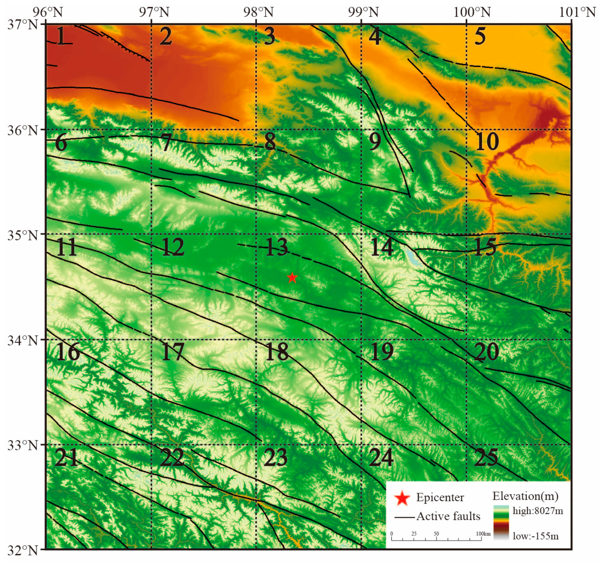
2.1. Study Earthquakes
2.2. Data
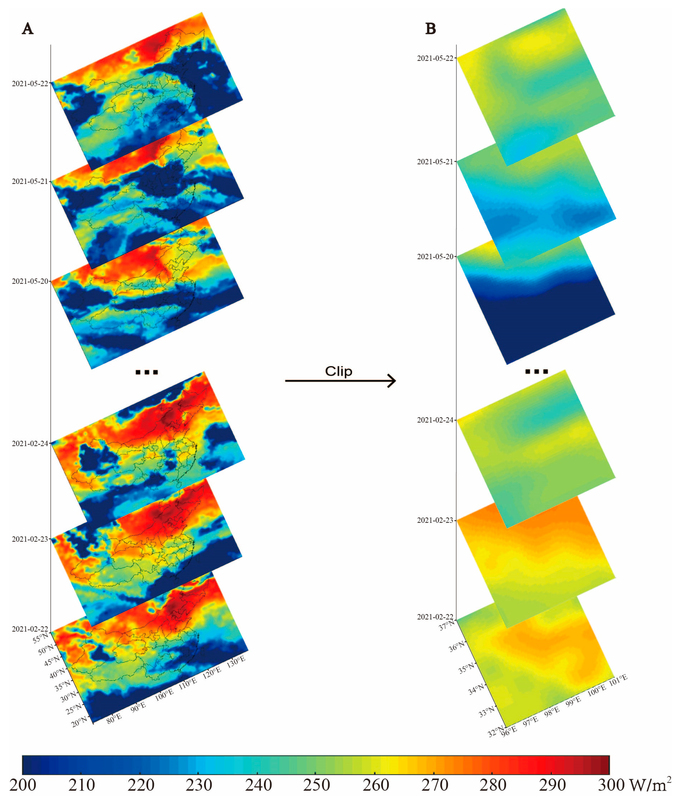
2.3. Data Preprocessing
3. Methods
3.1. Time Series Forecasting Models
3.1.1. ARIMA
3.1.2. SVM
3.1.3. XGBoost
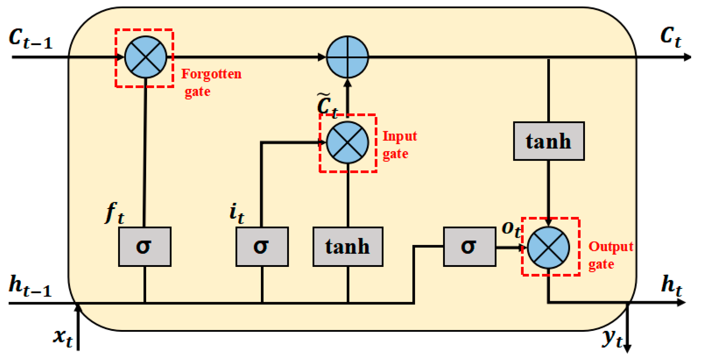
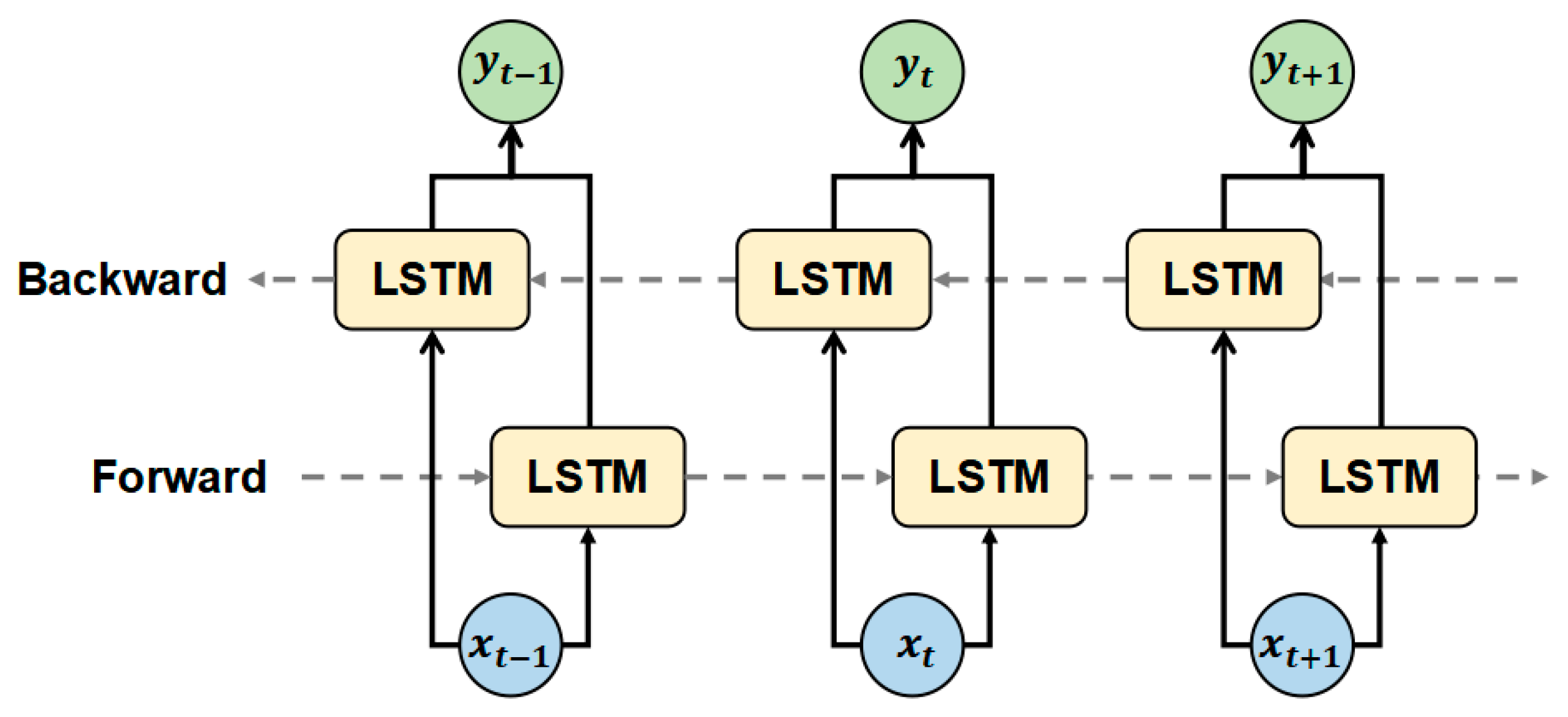
3.1.4. LSTM/BILSTM
3.2. Model Performance Comparison
3.3. Time Series Similarity Analysis
3.3.1. ED
3.3.2. DTW
3.4. Abnormal Identification and Extraction
4. Results
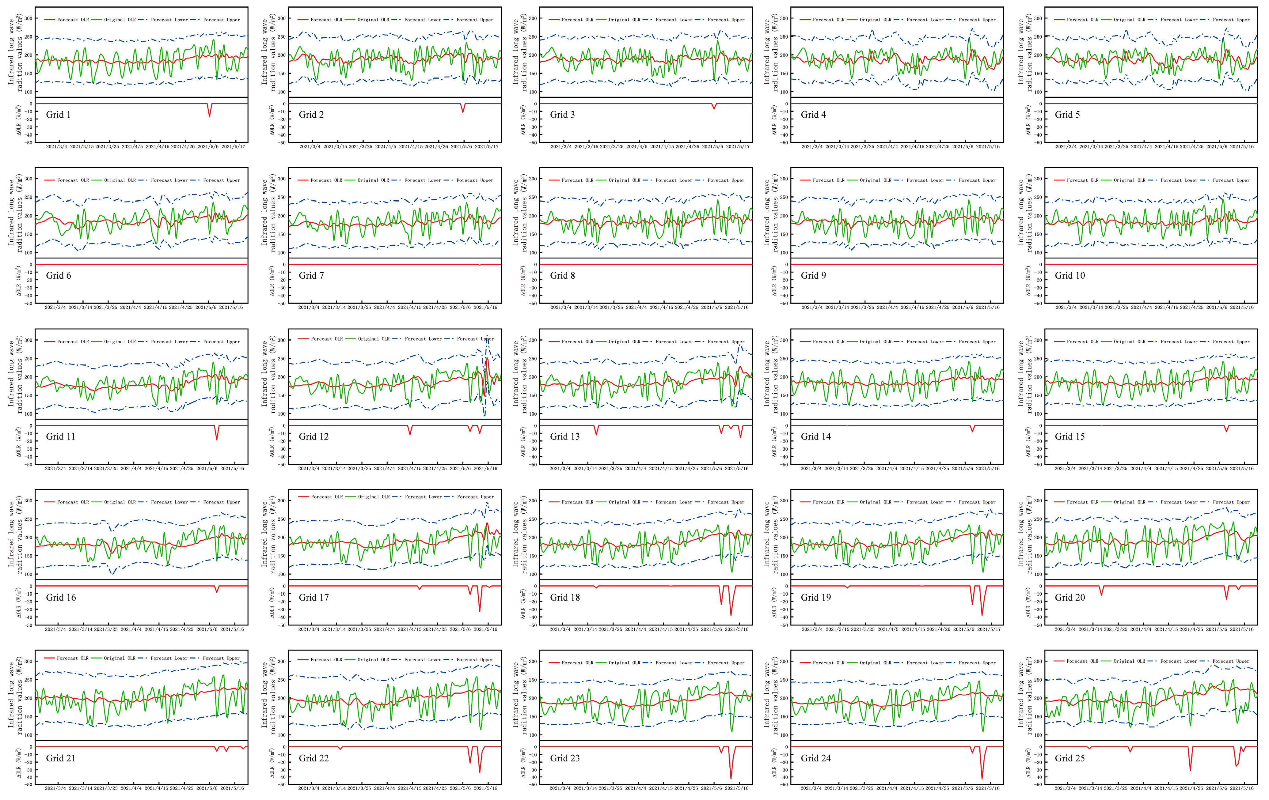
4.1. Model Performance
4.2. Similarity Comparison
4.2.1. ED Comparison
4.2.2. DTW Comparison
4.3. Abnormal Temporal and Spatial Characteristics
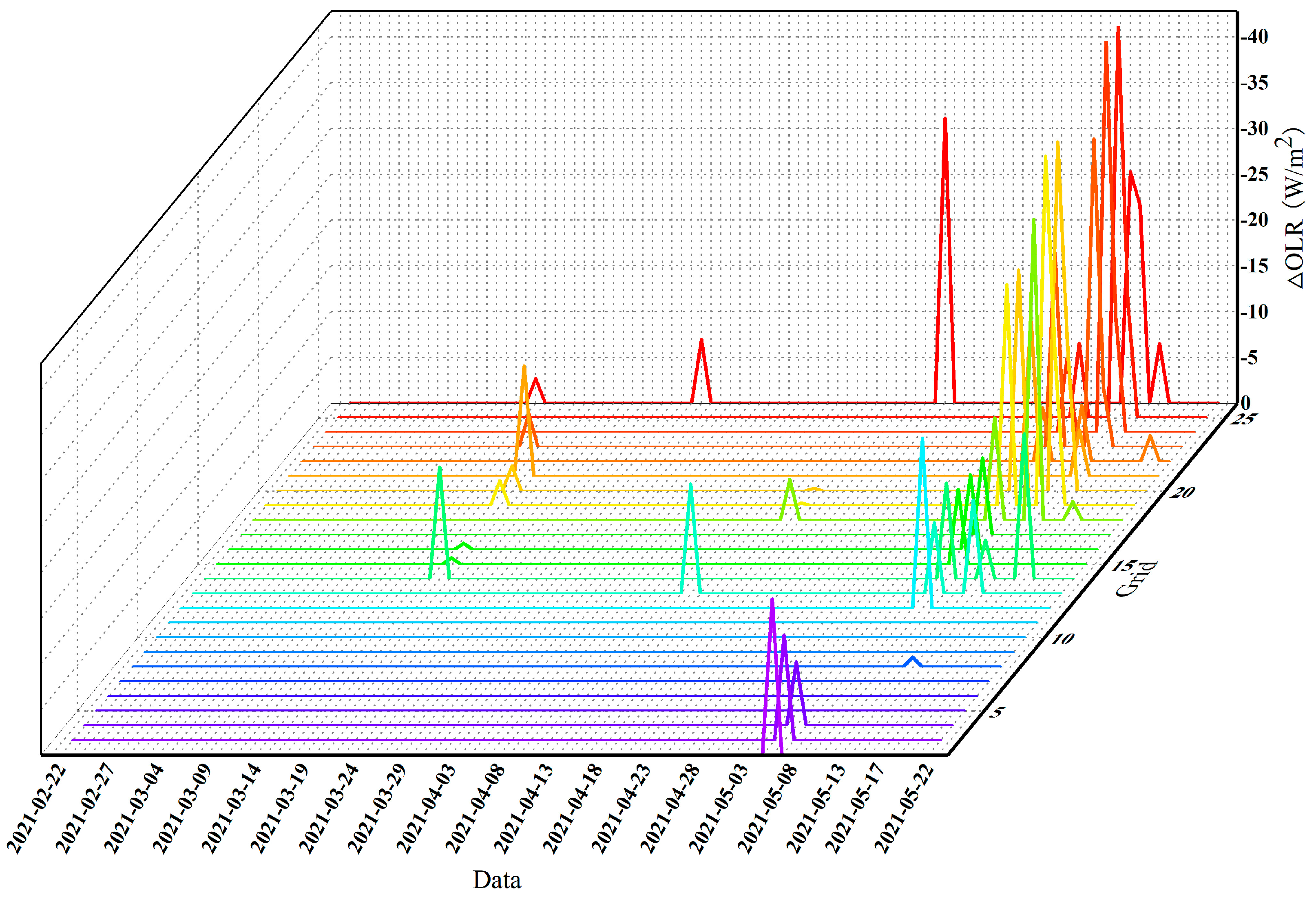
4.3.1. Temporal Scale Characteristics
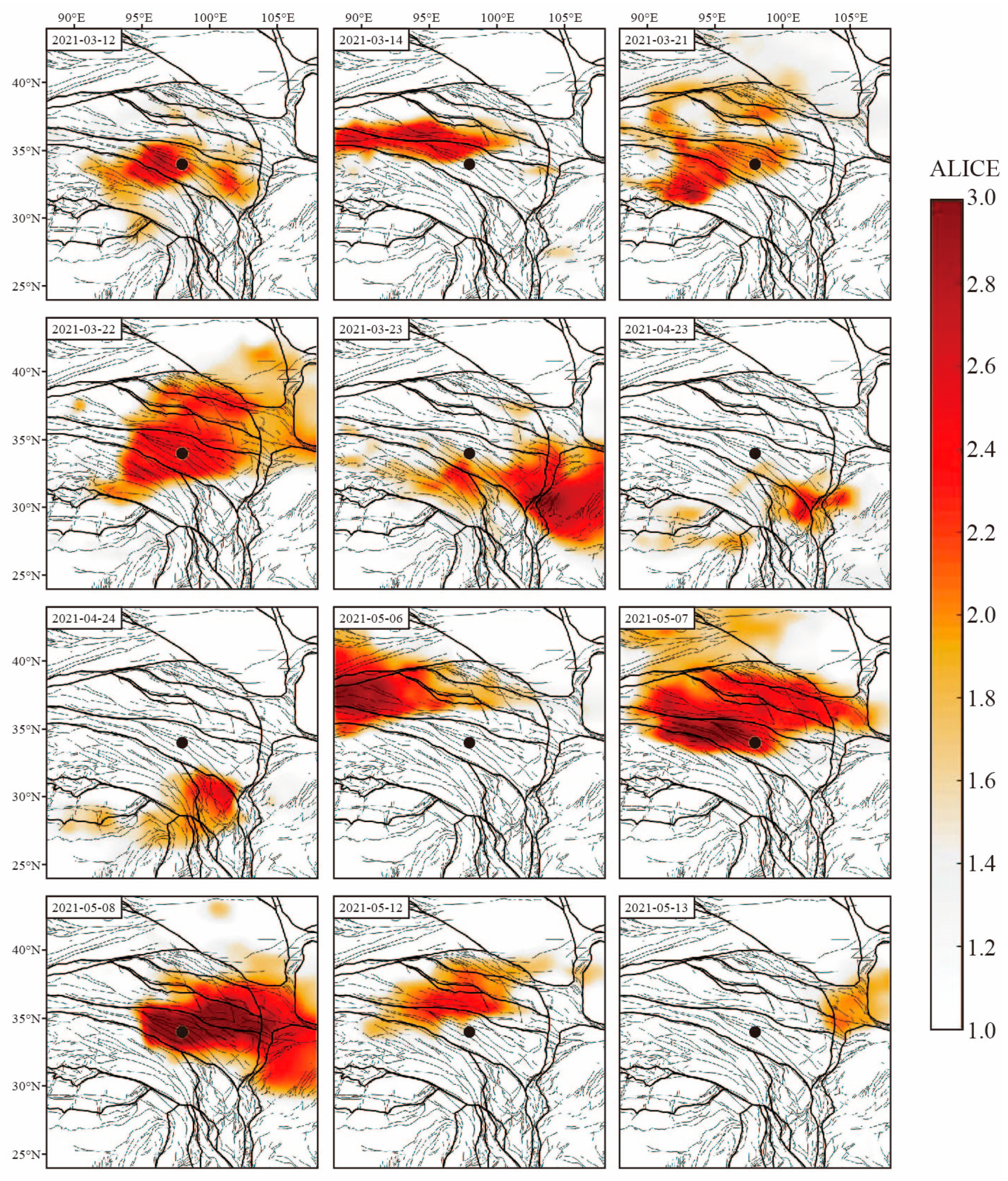
4.3.2. Spatial Scale Characteristics
5. Discussion
5.1. Consistency of LSTM Results with Traditional Methods
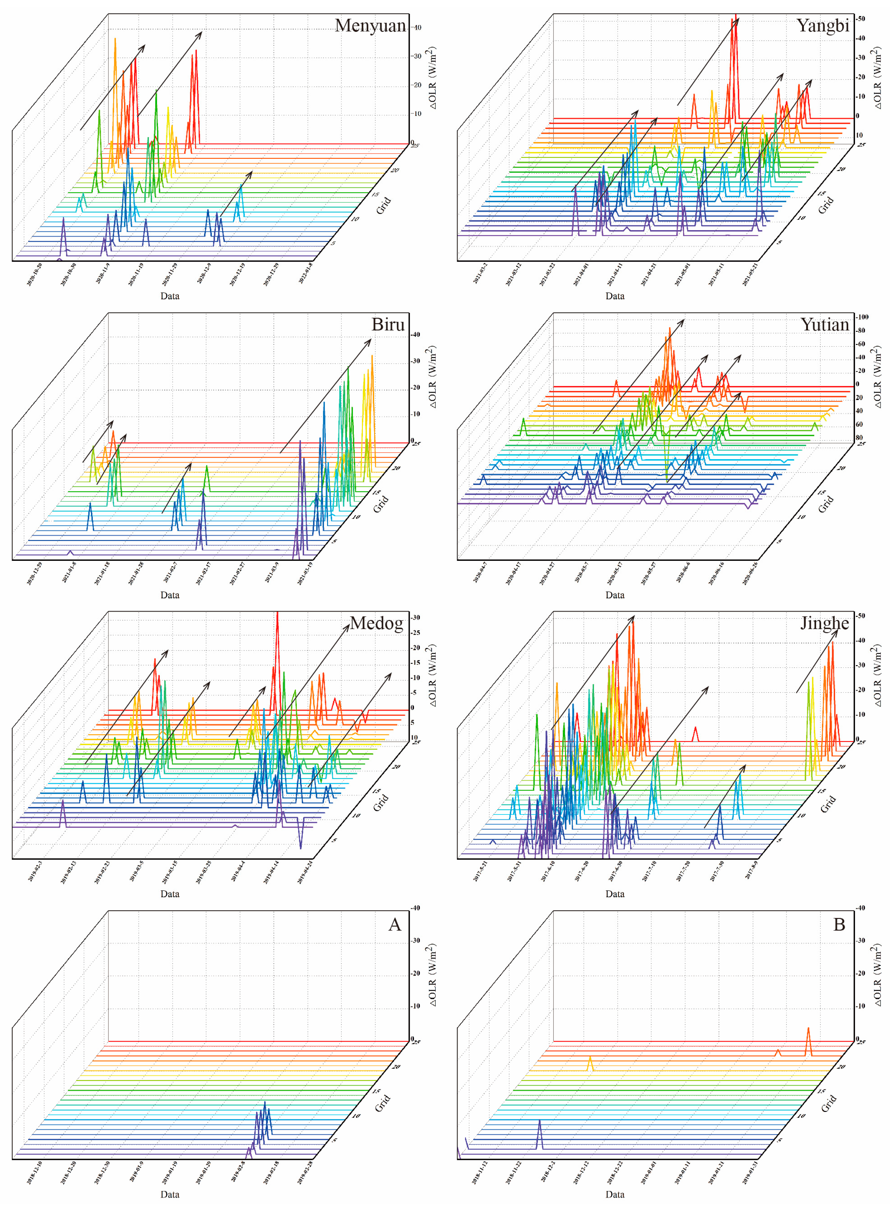
5.2. Robustness of the LSTM Model
5.3. Advantages of the LSTM Model
5.4. Multi-Parameter Coupling Relationship and Anomaly Generation Mechanism Analysis before Earthquake
6. Conclusions
- (1)
- The two time series similarity analysis methods proved that the similarity between the time series of the actual values at the time of the aseismic and the predicted values were better than those before the earthquake, indicating an anomalous period.
- (2)
- The results of the RMSE-based accuracy evaluation show that, among the five selected time series prediction models, the prediction performance of the LSTM model is better than several other time series models, which is attributed to the strong learning ability of the deep-learning model on data features. After accepting the input time series data, the LSTM layer, utilizing its ability to process the contextual information and the memory capability, has the potential to dig in and capture the potential nonlinear features in the time-series data.
- (3)
- The anomalies are extracted, and the temporal and spatial change characteristics of the anomalies are analyzed using 95% confidence intervals. On the time scale, the earliest anomalies appeared seventy days before the earthquake. The closer to the moment of the earthquake, the higher the frequency of anomalies, the wider the coverage area, and the higher the intensity; the anomalies exceeded the lower limit of the confidence interval of 40 W/m2 on the ninth day before the earthquake. On the spatial scale, the anomalies are concentrated in the southern and southeastern parts of the epicenter, where the distribution of fault zones is denser, and are less frequent in the northern part of the epicenter, where the fault zones are sparse, which suggests that tectonic activity is potentially related to the occurrence of earthquakes and the emergence of radiation anomalies. In addition, it is worth noting that the selection of the confidence interval affects the extraction of anomalies, and as the threshold setting of the confidence interval increases, some small amplitude chance anomalies unrelated to earthquakes will be filtered out, and the results will be more reliable.
- (4)
- The method of exploring the pre-earthquake signals of the Madoi earthquake with deep-learning prediction OLR time series is feasible. The application of the method achieved the expected purpose. After the occurrence of anomalies, we should focus on the rupture zones and faults in a locking state around the relevant geological bodies, which may be advantageous locations for the origin of future strong earthquakes. At present, only a complete experiment has been carried out for the Madoi earthquake, and this method will be applied to the processing and analysis of other moderate and strong earthquakes in the future to further verify the feasibility of the method of exploring pre-earthquake signals by predicting OLR time series with deep learning.
Author Contributions
Funding
Institutional Review Board Statement
Informed Consent Statement
Data Availability Statement
Acknowledgments
Conflicts of Interest
References
- Zhang, Y.; Meng, Q.; Wang, Z.; Lu, X.; Hu, D. Temperature Variations in Multiple Air Layers before the Mw 6.2 2014 Ludian Earthquake, Yunnan, China. Remote Sens. 2021, 13, 884. [Google Scholar] [CrossRef]
- Cui, Y.; Ouzounov, D.; Hatzopoulos, N.; Sun, K.; Zou, Z.; Du, J. Satellite observation of CH4 and CO anomalies associated with the Wenchuan MS 8.0 and Lushan MS 7.0 earthquakes in China. Chem. Geol. 2017, 469, 185–191. [Google Scholar] [CrossRef]
- Singh, R.; Cervone, G.; Kafatos, M.; Prasad, A.K.; Sahoo, A.K.; Sun, D.; Tang, D.L.; Yang, R. Multi-sensor studies of the Sumatra earthquake and tsunami of December 26 2004. Int. J. Remote Sens. 2007, 28, 2885–2896. [Google Scholar] [CrossRef]
- Xiong, B.; Li, X.; Wang, Y.Q.; Zhang, H.M.; Liu, Z.J.; Ding, F.; Zhao, B.Q. Prediction of ionospheric TEC over China based on long and short-term memory neural network. Chin. J. Geophys. -Chin. Ed. 2022, 65, 2365–2377. [Google Scholar]
- Kang, C.L.; Han, Y.B.; Liu, D.F.; Cao, Z.Q. The OLR anomaly and mechanism before Tibet earthquake(M6.9). Prog. Geophys. 2008, 23, 1703–1708. [Google Scholar]
- Ouzounov, D.; Liu, D.; Kang, C.; Cervone, G.; Kafatos, M.; Taylor, P. Outgoing long wave radiation variability from IR satellite data prior to major earthquakes. Tectonophysics 2007, 431, 211–220. [Google Scholar] [CrossRef]
- Pulinets, S.; Ouzounov, D. The Possibility of Earthquake Forecasting: Learning from Nature; Institute of Physics Books; IOP Publishing: Bristol, UK, 2018; p. 168. [Google Scholar]
- Sun, H.B.; Zhang, X.D. Primary exploration in relating to earthquake and Outgoing long-wave Radiation. Plateau Earthq. Res. 1990, 24, 6873. [Google Scholar]
- Liu, D.F.; Kang, C.L. Predicting heavy disasters by outgoing longwave radiation (OLR) of the earth. Earth Sci. Front. 2003, 2, 427–435. [Google Scholar]
- Jing, F.; Shen, X.H.; Kang, C.L.; Xiong, P. Variations of multi-parameter observations in atmosphere related to earthquake. Nat. Hazards Earth Syst. Sci. 2013, 13, 27–33. [Google Scholar] [CrossRef]
- Sun, K.; Shan, X.J.; Ouzounov, D.; Shen, X.H.; Jing, F. Analyzing long wave radiation data associated with the 2015 Nepal earthquakes based on Multi-orbit satellite observations. Chin. J. Geophys.-Chin. Ed. 2017, 60, 3457–3465. [Google Scholar]
- Tramutoli, V.; Aliano, C.; Corrado, R.; Filizzola, C.; Genzano, N.; Lisi, M.; Martinelli, G.; Pergola, N. On the possible origin of thermal infrared radiation (TIR) anomalies in earthquake-prone areas observed using robust satellite techniques (RST). Chem. Geol. 2013, 339, 157–168. [Google Scholar] [CrossRef]
- Jing, F.; Shen, X.H.; Wang, H.; Kang, C.L.; Xiong, P. Infrared characteristics analysis of the 2015 Nepal Ms8.1 earthquake. Acta Seismol. Sin. 2016, 38, 429–437. [Google Scholar]
- Guo, X.; Zhang, Y.S.; Zhong, M.J.; Shen, W.R.; Wei, C.X. Variation characteristics of OLR for the Wenchuan earthquake. Chin. J. Geophys. 2010, 53, 2688–2695. [Google Scholar]
- Al Banna, M.H.; Abu Taher, K.; Kaiser, M.S.; Mahmud, M.; Rahman, M.S.; Hosen, A.S.M.S.; Cho, G.H. Application of Artificial Intelligence in Predicting Earthquakes: State-of-the-Art and Future Challenges. IEEE Assess 2020, 08, 192880–192923. [Google Scholar] [CrossRef]
- Wang, Q.L.; Guo, Y.F.; Yu, L.X.; Li, P. Earthquake Prediction Based on Spatio-Temporal Data Mining: An LSTM Network Approach. IEEE Trans. Emerg. Top. Comput. 2020, 8, 148–158. [Google Scholar] [CrossRef]
- Sadhukhan, B.; Chakraborty, S.; Mukherjee, S. Predicting the magnitude of an impending earthquake using deep learning techniques. Earth Sci. Inform. 2023, 16, 803–823. [Google Scholar] [CrossRef]
- Senturk, E.; Saqib, M.; Adil, M.A. A Multi-Network based Hybrid LSTM model for ionospheric anomaly detection: A case study of the Mw 7.8 Nepal earthquake. Adv. Space Res. 2022, 70, 440–455. [Google Scholar] [CrossRef]
- Xiong, P.; Long, C.; Zhou, H.Y.; Battiston, R.; Zhang, X.M.; Shen, X.H. Identification of electromagnetic pre-earthquake perturbations from the DEMETER data by machine learning. Remote Sens. 2020, 12, 3643. [Google Scholar] [CrossRef]
- Draz, M.U.; Shah, M.; Jamjareegulgarn, P.; Shahzad, R.; Hasan, A.M.; Ghamry, N.A. Deep machine learning based possible atmospheric and Ionospheric precursors of the 2021 Mw 7.1 Japan Earthquake. Remote Sens. 2023, 15, 1904. [Google Scholar] [CrossRef]
- Chen, Q.F.; Zheng, D.L.; Che, S. Earthquake Cases in China (1992–1994); Seismological Press: Beijing, China, 2002. [Google Scholar]
- Chen, Q.F.; Zheng, D.L.; Liu, G.P.; Li, M. Earthquake Cases in China (1995–1996); Seismological Press: Beijing, China, 2002. [Google Scholar]
- Chen, Q.F.; Zheng, D.L.; Gao, R.S. Earthquake Cases in China (1997–1999); Seismological Press: Beijing, China, 2002. [Google Scholar]
- Jiang, H.K.; Fu, H.; Yang, M.L.; Ma, H.S. Earthquake Cases in China (2003–2006); Seismological Press: Beijing, China, 2014. [Google Scholar]
- Jiang, H.K.; Yang, M.L.; Fu, H. Earthquake Cases in China (2011–2012); Seismological Press: Beijing, China, 2018. [Google Scholar]
- Jing, F.; Shen, X.H.; Kang, C.L.; Meng, Q.Y.; Xiong, P. Preliminary Analysis of the Background Features of Outgoing Longwave Radiation in China. Earthquake 2009, 29, 90–97. [Google Scholar]
- Lu, X.; Meng, Q.; Gu, X.; Zhang, X.; Xie, T.; Geng, F. Thermal infrared anomalies associated with multi-year earthquakes in the Tibet region based on China’s FY-2E satellite data. Adv. Space Res. 2016, 58, 989–1001. [Google Scholar] [CrossRef]
- Song, D.M.; Zang, L.; Shan, X.J.; Yuan, Y.; Cui, J.Y.; Shao, H.M.; Shen, C.; Shi, H.T. A study on the algorithm for extracting earthquake thermal infrared anomalies based on the yearly trend of LST. Seismol. Geol. 2016, 38, 680–695. [Google Scholar]
- Eleftheriou, A.; Filizzola, C.; Genzano, N.; Lacava, T.; Lisi, M.; Paciello, R.; Pergola, N.; Vallianatos, F.; Tramutoli, V. Long-Term RST Analysis of Anomalous TIR Sequences in Relation with Earthquakes Occurred in Greece in the Period 2004–2013. Pure Appl. Geophys. 2016, 173, 285–303. [Google Scholar] [CrossRef]
- Box, G.E.P.; Jenkins, G.M. Time Series Analysis: Forecasting and Control; Holden Day: San Francisco, CA, USA, 1976. [Google Scholar]
- Zhu, J.B.; Song, J.D.; Li, S.Y. Magnitude estimation for the February 13, 2021 Mj7.3 earthquake near the coast of Fukushima Japan based on support vector machine. World Earthq. Eng. 2021, 37, 74–81. [Google Scholar]
- Wang, T.T.; Bian, Y.J.; Zhang, Y.X.; Hou, X.L. Classification of earthquakes, explosions and mining-induced earthquakes based on XGBoost algorithm. Comput. Geosci. 2023, 170, 105242. [Google Scholar] [CrossRef]
- Hsu, T.Y.; Pratomo, A. Early Peak Ground Acceleration Prediction for On-Site Earthquake Early Warning Using LSTM Neural Network. Front. Earth Sci. 2022, 10, 911947. [Google Scholar] [CrossRef]
- Lin, H.; Zhang, S.; Li, Q.; Li, Y.; Li, J.; Yang, Y. A new method for heart rate prediction based on LSTM-BiLSTM-Att. Measurement 2023, 207, 112384. [Google Scholar] [CrossRef]
- Xiong, P.; Zhai, D.L.; Long, C.; Zhou, H.Y.; Zhang, X.M.; Shen, X.H. Long Short-Term Memory Neural Network for Ionospheric Total Electron Content Forecasting Over China. Space Weather 2021, 19, 2365–2377. [Google Scholar] [CrossRef]
- Nicolis, O.; Plaza, F.; Salas, R. Prediction of intensity and location of seismic events using deep learning. Spat. Stat. 2021, 42, 100442. [Google Scholar] [CrossRef]
- Chen, S.P.; Yin, L.; Liang, S.M.; Hu, X.Y.; Yu, X.Y. Application of Deep Learning to Predict GPS Time Series in Exploring Precursors of Menyuan Ms6.4 Earthquake. J. Geod. Geodyn. 2020, 40, 1248–1253. [Google Scholar]
- Zhai, D.L.; Zhang, X.M.; Xiong, P. Detecting Thermal Anomalies of Earthquake Process Within Outgoing Longwave Radiation Using Time Series Forecasting Models. Ann. Geophys. 2020, 63, 548. [Google Scholar] [CrossRef]
- Zhang, X.H.; Ren, X.D.; Wu, F.B.; Chen, Y.Y. A new method for detection of pre-earthquake ionospheric anomalies. Chin. J. Geophys.-Chin. Ed. 2013, 56, 441–449. [Google Scholar]
- Tramutoli, V. Robust AVHRR techniques (RAT) for environmental monitoring: Theory and applications. Proc. SPIE-Int. Soc. Opt. Eng. 1998, 3496, 101–113. [Google Scholar]
- Di Bello, G.; Filizzola, C.; Lacava, T.; Marchese, F.; Pergola, N.; Pietrapertosa, C.; Piscitelli, S.; Scaffidi, I.; Tramutoli, V. Robust satellite techniques for volcanic and seismic hazards monitoring. Ann. Geophys. 2004, 47, 49–64. [Google Scholar]
- Genzano, N.; Aliano, C.; Filizzola, C.; Pergola, N.; Tramutoli, V. A robust satellite technique for monitoring seismically active areas: The case of Bhuj-Gujarat earthquake. Tectonophysics 2007, 431, 197–210. [Google Scholar] [CrossRef]
- Zhang, Y.; Meng, Q. A statistical analysis of TIR anomalies extracted by RSTs in relation to an earthquake in the Sichuan area using MODIS LST data. Nat. Hazards Earth Syst. Sci. 2019, 19, 535–549. [Google Scholar] [CrossRef]
- Kang, C.L.; Chen, Z.W.; Chen, L.Z.; Tian, Q.J.; Liu, D.F. Analysis on the satellite infrared anomaly feature before west to Kunlun Mountain Pass M8.1 earthquake. China Earthq. Eng. J. 2003, 25, 12–15. [Google Scholar]
- Cui, J.; Shen, X.H.; Zhang, J.F.; Ma, W.Y.; Chu, W. Analysis of spatiotemporal variations in middle-tropospheric to upper-tropospheric methane during the Wenchuan MS = 8.0 earthquake by three indices. Nat. Hazards Earth Syst. Sci. 2019, 19, 2841–2854. [Google Scholar] [CrossRef]
- Meng, Q.; Zhang, Y. Discovery of spatial-temporal causal interactions between thermal and methane anomalies associated with the Wenchuan earthquake. Eur. Phys. J.-Spec. Top. 2021, 230, 247–261. [Google Scholar] [CrossRef]
- Guo, X.; Zou, Y.; Zhang, X.; Wang, Y. Anomalies in Outgoing Long-Wave Radiation for Several Strong Earthquakes in Mainland China. China Earthq. Eng. J. 2019, 41, 1221–1227. [Google Scholar]
- Han, S.S.; Tan, K.; Lu, X.F.; Zhang, C.H.; Li, Q. Analysis of Strain Evolution Characteristics before the 2021 Maduo 7.4 Earthquake in Qinghai. J. Geod. Geodyn. 2023, 43, 641–645. [Google Scholar]
- Deng, M.D.; Geng, N.G.; Cui, C.Y.; Zhi, Y.Q.; Fan, Z.F.; Ji, Q.Q. The Study on the Variation of Thermal State of Rocks Caused by the Variation of Stress State of Rocks. Earthq. Res. China 1997, 02, 85–91. [Google Scholar]
- Du, X.H.; Zhang, X.M. Ionospheric Disturbances Possibly Associated with Yangbi Ms6.4 and Maduo Ms7.4 Earthquakes in China from China Seismo Electromagnetic Satellite. Atmosphere 2022, 13, 438. [Google Scholar] [CrossRef]
- Zhang, X.M.; Liu, J.; Zhou, Y.L.; Du, X.H. The ionospheric Perturbations Around Yunnan Yangbi Ms6.4 and Qinghai Maduo Ms7.4 Earthquakes in 2021. Earthquake 2022, 42, 1–20. [Google Scholar]
- Wang, S.Y.; Tian, H.; Ma, K.X.; Yu, C.; Ma, W.Y.; Yu, H.Z. Correlation between short-term and imminent anomalies of LURR and OLR before the Maduo Ms7.4 earthquake in Qinghai Province, 2021. China Earthq. Eng. J. 2021, 43, 847–852. [Google Scholar]
- Su, W.G.; Liu, L.; Sun, X.H. Characteristics of underground fluid anomalies in Zuoshu station before Maduo Ms7.4 and Menyuan Ms6.9 earthquakes. China Earthq. Eng. J. 2022, 44, 700–706, 712. [Google Scholar]
- Jing, F.; Zhang, L.; Singh, R.P. Pronounced Changes in Thermal Signals Associated with the Madoi (China) M 7.3 Earthquake from Passive Microwave and Infrared Satellite Data. Remote Sens. 2022, 14, 2539. [Google Scholar] [CrossRef]
- Luo, B.S.; Bai, Z.X.; Li, Y.F. Analysis on abnormal characteristic of water radon in HuangYuan station before and after the Ms 7.4 Maduo earthquake in 2021. Plateau Earthq. Res. 2022, 34, 53–57. [Google Scholar]
- Pulinets, S.; Ouzounov, D. Lithosphere-Atmosphere-Ionosphere Coupling (LAIC) model—An unified concept for earthquake precursors validation. J. Asian Earth Sci. 2011, 41, 371–382. [Google Scholar] [CrossRef]


| Grid | ARIMA | SVM | XGBoost | LSTM | BILSTM |
|---|---|---|---|---|---|
| 1 | 34.2619 | 35.1532 | 30.8762 | 30.5294 | 33.6217 |
| 2 | 53.1949 | 36.1017 | 34.9021 | 30.7129 | 32.3657 |
| 3 | 58.2728 | 33.0449 | 31.8505 | 26.7471 | 27.9391 |
| 4 | 44.444 | 30.2318 | 28.8857 | 26.7325 | 27.6086 |
| 5 | 44.444 | 30.2318 | 28.8857 | 26.7325 | 27.6086 |
| 6 | 50.9688 | 40.6984 | 35.6925 | 33.1588 | 34.6644 |
| 7 | 53.0276 | 34.4316 | 36.2105 | 32.0643 | 33.0467 |
| 8 | 47.2451 | 34.6952 | 35.5667 | 30.8911 | 31.451 |
| 9 | 53.2237 | 32.278 | 33.349 | 30.1235 | 29.7703 |
| 10 | 54.5762 | 35.9806 | 38.6714 | 32.6847 | 32.0692 |
| 11 | 53.5756 | 40.6919 | 39.8142 | 36.5470 | 37.1474 |
| 12 | 53.5756 | 40.6919 | 39.8142 | 36.5470 | 37.1474 |
| 13 | 70.4604 | 38.8847 | 36.4824 | 33.1946 | 34.5191 |
| 14 | 41.412 | 40.2266 | 37.6286 | 36.5276 | 36.032 |
| 15 | 41.7221 | 41.2979 | 41.9942 | 36.7073 | 36.7855 |
| 16 | 44.5678 | 40.9163 | 37.4803 | 35.4564 | 34.5752 |
| 17 | 58.5795 | 42.6388 | 37.4096 | 35.6641 | 37.3662 |
| 18 | 52.4613 | 39.7556 | 37.5302 | 34.8795 | 37.4875 |
| 19 | 47.4852 | 37.6338 | 37.0222 | 36.4709 | 37.1824 |
| 20 | 39.4942 | 39.1195 | 40.4514 | 37.6639 | 36.3644 |
| 21 | 61.4502 | 41.8658 | 40.5014 | 38.3213 | 37.3602 |
| 22 | 61.4502 | 41.8658 | 40.5014 | 38.3213 | 37.3602 |
| 23 | 52.6675 | 35.1916 | 34.3085 | 31.4399 | 33.413 |
| 24 | 42.6541 | 32.3148 | 32.4968 | 31.4682 | 32.2569 |
| 25 | 38.0416 | 32.2304 | 34.0134 | 31.7403 | 31.5389 |
| Total | 1253.2563 | 928.1726 | 902.3391 | 831.3261 | 846.6816 |
| Gird | ED in the Aseismic Period | ED in the Seismic Period | Difference Value |
|---|---|---|---|
| 1 | 186.8928 | 215.2030 | 28.3102 |
| 2 | 182.2871 | 243.9496 | 61.6625 |
| 3 | 198.2106 | 222.8911 | 24.6805 |
| 4 | 193.0780 | 222.0978 | 29.0198 |
| 5 | 193.0780 | 222.0978 | 29.0198 |
| 6 | 200.2466 | 218.4609 | 18.2143 |
| 7 | 193.9372 | 231.1959 | 37.2587 |
| 8 | 200.1804 | 239.3742 | 39.1938 |
| 9 | 200.1804 | 239.3742 | 39.1938 |
| 10 | 210.2695 | 231.7173 | 21.4478 |
| 11 | 205.3519 | 218.5727 | 13.2208 |
| 12 | 216.1626 | 243.7730 | 27.6104 |
| 13 | 210.8625 | 254.2664 | 43.4039 |
| 14 | 193.5884 | 244.6240 | 51.0356 |
| 15 | 193.5884 | 244.6240 | 51.0356 |
| 16 | 193.7733 | 216.9230 | 23.1497 |
| 17 | 199.9631 | 259.6670 | 59.7039 |
| 18 | 188.1746 | 253.0382 | 64.8636 |
| 19 | 188.1746 | 253.0382 | 64.8636 |
| 20 | 214.1401 | 287.3047 | 73.1646 |
| 21 | 222.7757 | 282.6755 | 59.8998 |
| 22 | 217.8504 | 294.7557 | 76.9053 |
| 23 | 180.2219 | 262.8554 | 82.6335 |
| 24 | 180.2219 | 262.8554 | 82.6335 |
| 25 | 210.8567 | 296.3231 | 85.4664 |
| Gird | DTW in the Aseismic Period | DTW in the Seismic Period | Difference Value |
|---|---|---|---|
| 1 | 1048.3101 | 1122.6331 | 74.323 |
| 2 | 1192.8760 | 1458.1691 | 265.2931 |
| 3 | 1233.5800 | 1460.4359 | 226.8559 |
| 4 | 1201.0691 | 1287.7728 | 86.7037 |
| 5 | 1201.0691 | 1287.7728 | 86.7037 |
| 6 | 1252.1896 | 1292.0052 | 39.8156 |
| 7 | 1218.4646 | 1584.6326 | 366.168 |
| 8 | 1159.1498 | 1524.3408 | 365.191 |
| 9 | 1159.1498 | 1524.3408 | 365.191 |
| 10 | 1328.1454 | 1423.4520 | 95.3066 |
| 11 | 1306.5641 | 1342.0472 | 35.4831 |
| 12 | 1258.7495 | 1451.5585 | 192.809 |
| 13 | 1262.1207 | 1613.9854 | 351.8647 |
| 14 | 1150.4503 | 1752.4018 | 601.9515 |
| 15 | 1150.4503 | 1752.4018 | 601.9515 |
| 16 | 1213.2118 | 1244.7485 | 31.5367 |
| 17 | 1120.0947 | 1756.5435 | 636.4488 |
| 18 | 983.54445 | 1500.6782 | 517.13375 |
| 19 | 983.54445 | 1500.6782 | 517.13375 |
| 20 | 1331.7225 | 1870.4373 | 538.7148 |
| 21 | 1252.8426 | 2052.9131 | 800.0705 |
| 22 | 1285.1753 | 2056.8329 | 771.6576 |
| 23 | 990.76198 | 1797.7720 | 807.01002 |
| 24 | 990.76198 | 1797.7720 | 807.01002 |
| 25 | 1326.1863 | 1954.9361 | 628.7498 |
| Date (y-m-d) | Longitude (°E) | Latitude (°N) | Depth (km) | Magnitude (MS) | Location |
|---|---|---|---|---|---|
| 2022-01-08 | 101.26 | 37.77 | 10 | 6.9 | Menyuan, Qinghai |
| 2021-05-21 | 99.87 | 25.67 | 8 | 6.4 | Yangbi, Yunnan |
| 2021-03-19 | 92.74 | 31.94 | 10 | 6.1 | Biru, Tibet |
| 2020-06-26 | 82.33 | 35.73 | 10 | 6.4 | Yutian, Xinjiang |
| 2019-04-24 | 94.61 | 28.40 | 10 | 6.3 | Medog, Tibet |
| 2017-08-09 | 82.89 | 44.27 | 11 | 6.6 | Jinghe, Xinjiang |
| 2019-02-28 | 112 | 44 | — | — | A |
| 2019-01-31 | 83 | 40 | — | — | B |
Disclaimer/Publisher’s Note: The statements, opinions and data contained in all publications are solely those of the individual author(s) and contributor(s) and not of MDPI and/or the editor(s). MDPI and/or the editor(s) disclaim responsibility for any injury to people or property resulting from any ideas, methods, instructions or products referred to in the content. |
© 2023 by the authors. Licensee MDPI, Basel, Switzerland. This article is an open access article distributed under the terms and conditions of the Creative Commons Attribution (CC BY) license (https://creativecommons.org/licenses/by/4.0/).
Share and Cite
Zhang, J.; Sun, K.; Zhu, J.; Mao, N.; Ouzounov, D. Application of Model-Based Time Series Prediction of Infrared Long-Wave Radiation Data for Exploring the Precursory Patterns Associated with the 2021 Madoi Earthquake. Remote Sens. 2023, 15, 4748. https://doi.org/10.3390/rs15194748
Zhang J, Sun K, Zhu J, Mao N, Ouzounov D. Application of Model-Based Time Series Prediction of Infrared Long-Wave Radiation Data for Exploring the Precursory Patterns Associated with the 2021 Madoi Earthquake. Remote Sensing. 2023; 15(19):4748. https://doi.org/10.3390/rs15194748
Chicago/Turabian StyleZhang, Jingye, Ke Sun, Junqing Zhu, Ning Mao, and Dimitar Ouzounov. 2023. "Application of Model-Based Time Series Prediction of Infrared Long-Wave Radiation Data for Exploring the Precursory Patterns Associated with the 2021 Madoi Earthquake" Remote Sensing 15, no. 19: 4748. https://doi.org/10.3390/rs15194748
APA StyleZhang, J., Sun, K., Zhu, J., Mao, N., & Ouzounov, D. (2023). Application of Model-Based Time Series Prediction of Infrared Long-Wave Radiation Data for Exploring the Precursory Patterns Associated with the 2021 Madoi Earthquake. Remote Sensing, 15(19), 4748. https://doi.org/10.3390/rs15194748