
The Impact of Urbanization on the Supply–Demand Relationship of Ecosystem Services in the Yangtze River Middle Reaches Urban Agglomeration


 ,
, 

Abstract
:
1. Introduction
2. Materials and Methods
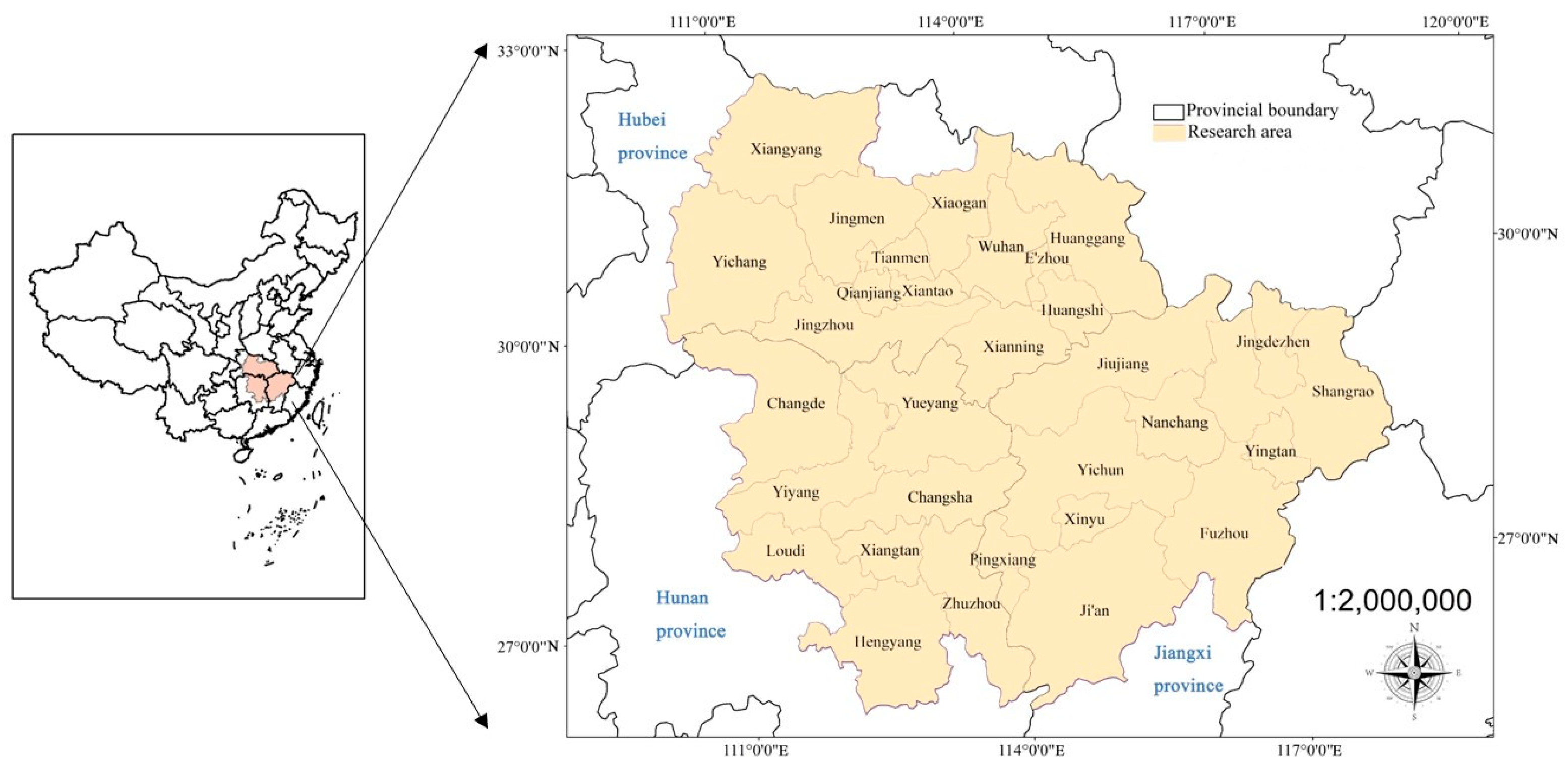
2.1. Study Area
2.2. ESs Supply and Demand
2.2.1. Food Production (Fo_P)
2.2.2. Carbon Storage (Ca_S)
2.2.3. Culture Service (Cu_S)
2.2.4. Total Ecosystem Service (TES) and Supply–Demand Index (SDI)
2.3. Geographical Detector Model
2.4. Moran’s I Index and Lisa Cluster
3. Results
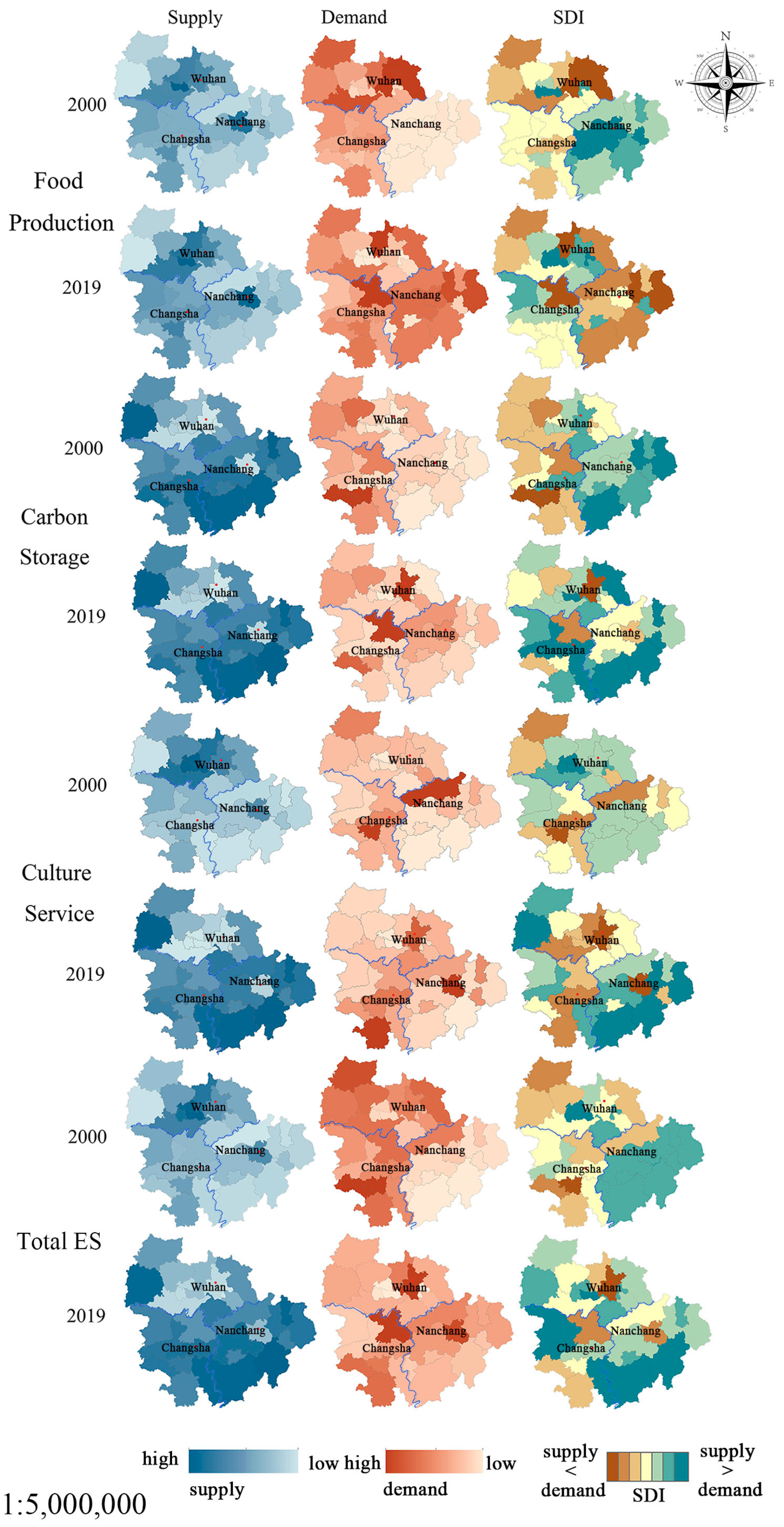
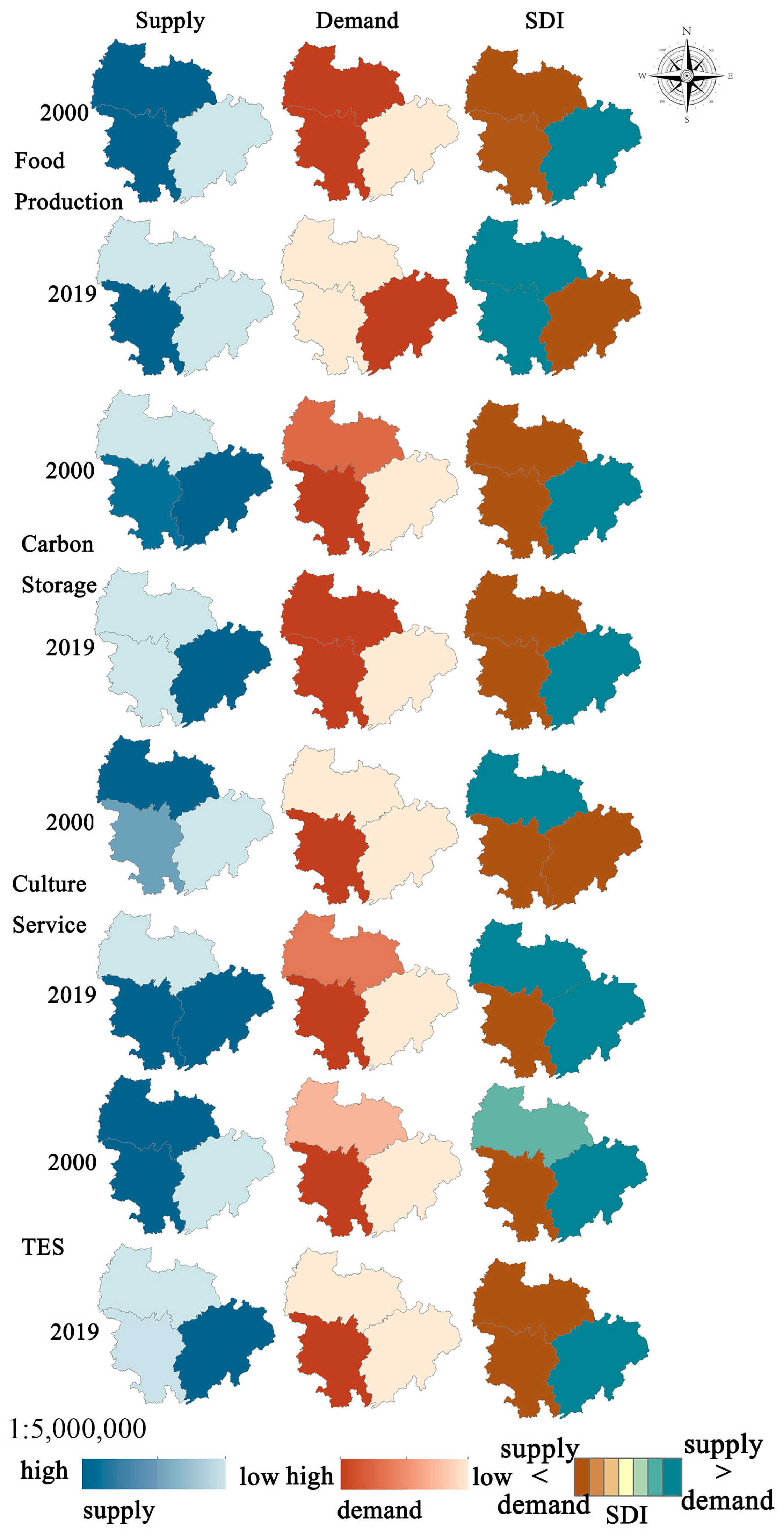
3.1. Variations in ES Supply–Demand at Different Scales
3.2. Simple Effect of Urbanization on ESs
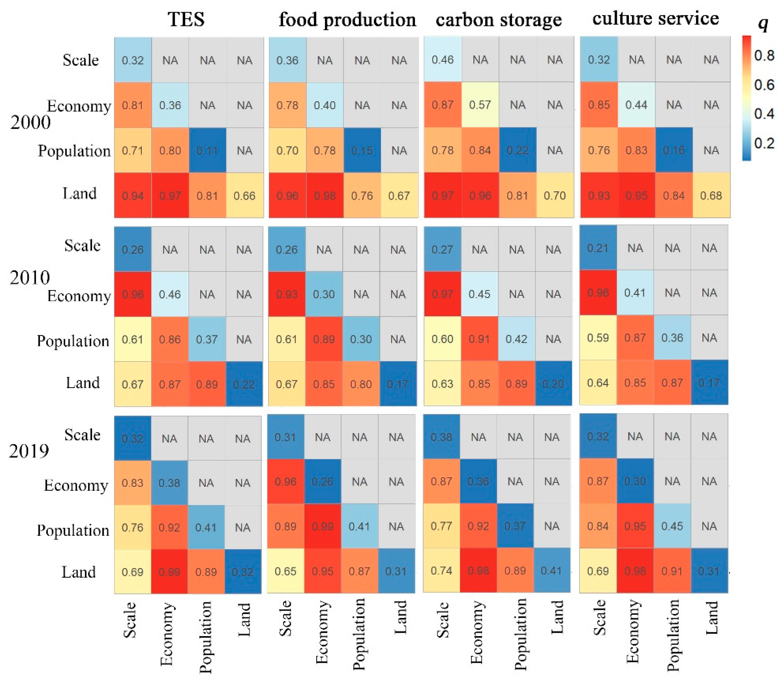
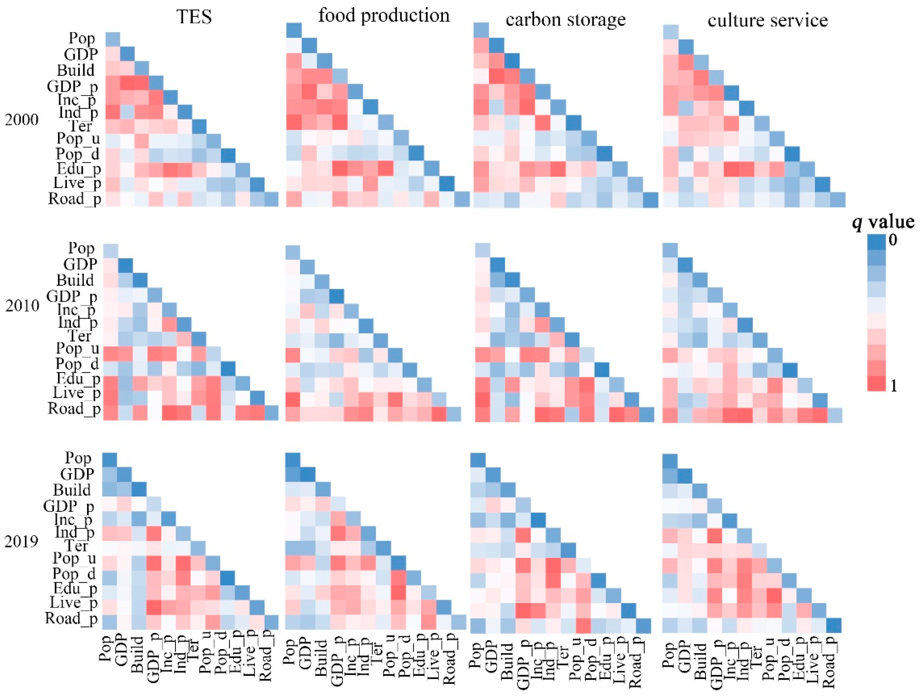
3.3. The Joint Effect of Urbanization on ESs
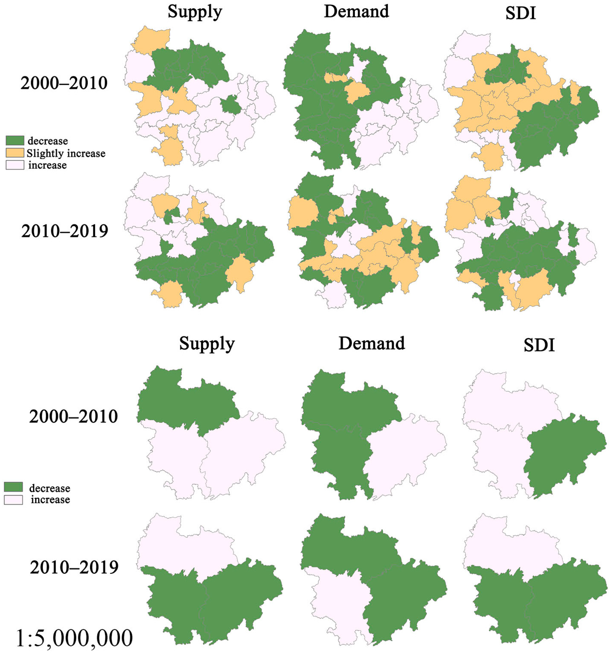
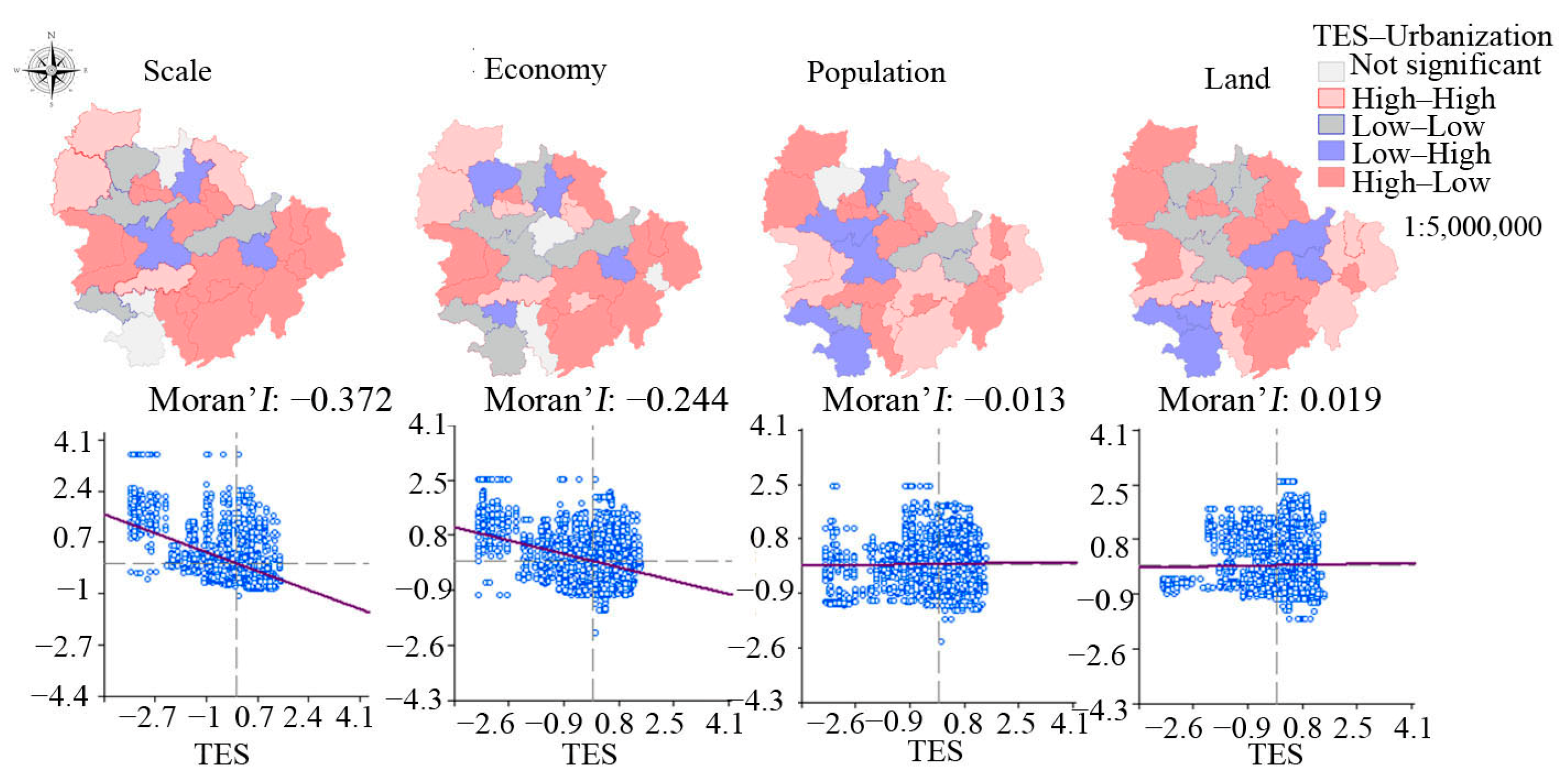
3.4. Spatial Visualization of Urbanization on SDI
4. Discussion
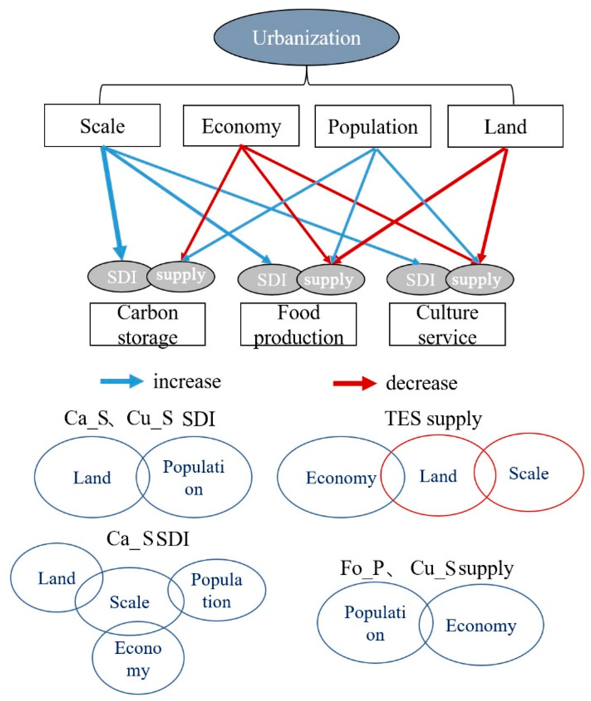
4.1. Driving Mechanism of Urbanization on Supply–Demand of ES
4.2. Policy Implications and Limitations
5. Conclusions
Author Contributions
Funding
Data Availability Statement
Conflicts of Interest
Appendix A

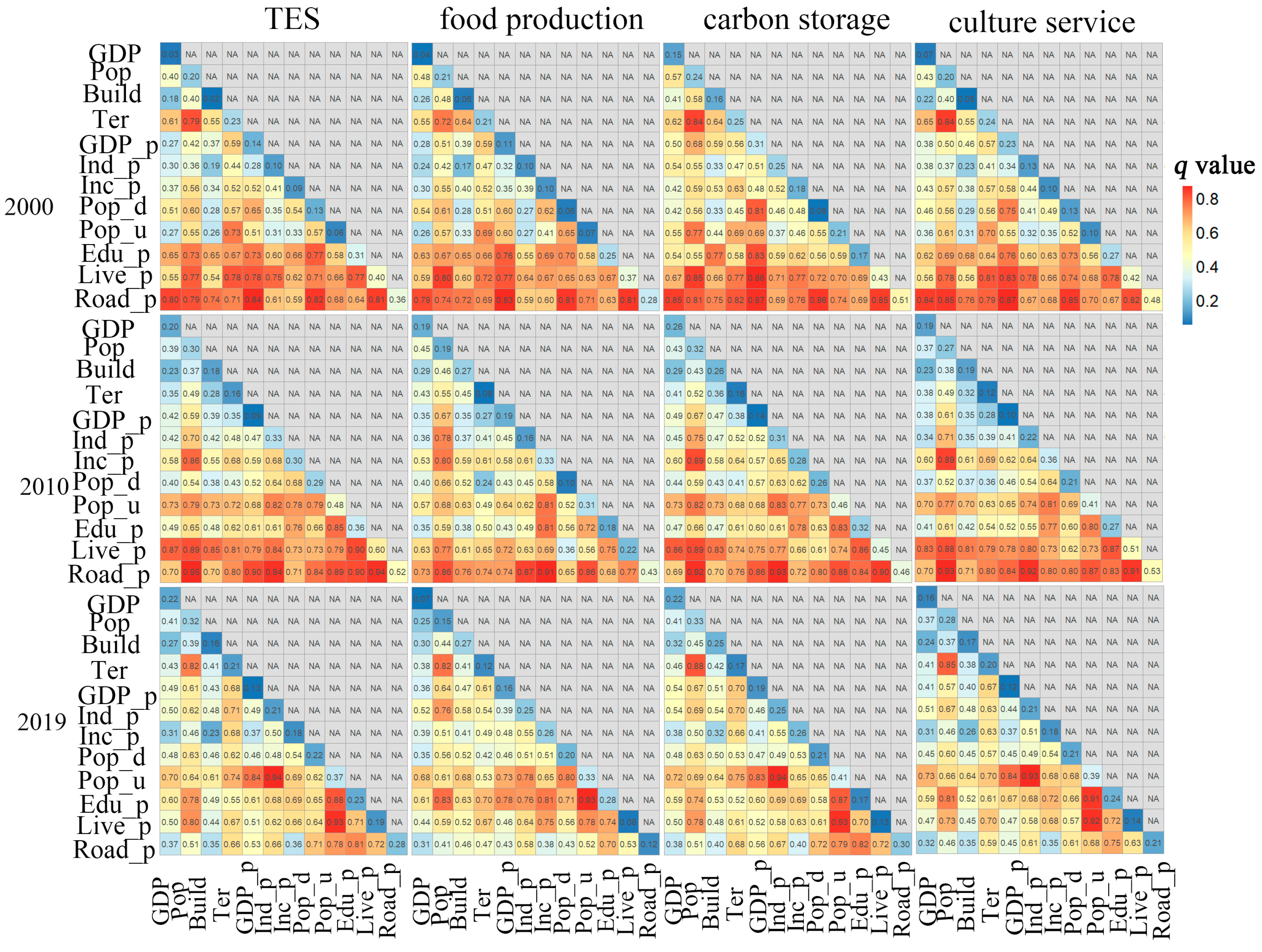
| Primary Indicators | Scale Urbanization | Economy Urbanization | Population Urbanization | Land Urbanization | |||||||||
|---|---|---|---|---|---|---|---|---|---|---|---|---|---|
| Year | GDP | Pop | Build | Ter | GDP_p | Ins_p | Inc_p | Pop_d | Pop_u | Edu_p | Liv_p | Road_p | |
| TES | 2000 | 0.03 | 0.20 | 0.02 | 0.23 | 0.14 | 0.10 | 0.09 | 0.13 | 0.06 | 0.31 | 0.40 | 0.36 |
| 2010 | 0.20 | 0.30 | 0.18 | 0.16 | 0.09 | 0.33 | 0.30 | 0.29 | 0.48 | 0.36 | 0.60 | 0.52 | |
| 2019 | 0.22 | 0.32 | 0.16 | 0.21 | 0.13 | 0.21 | 0.19 | 0.22 | 0.37 | 0.23 | 0.19 | 0.28 | |
| Food production | 2000 | 0.04 | 0.21 | 0.06 | 0.21 | 0.11 | 0.10 | 0.10 | 0.06 | 0.07 | 0.25 | 0.37 | 0.28 |
| 2010 | 0.19 | 0.19 | 0.27 | 0.08 | 0.19 | 0.16 | 0.33 | 0.10 | 0.31 | 0.18 | 0.22 | 0.43 | |
| 2019 | 0.07 | 0.15 | 0.27 | 0.12 | 0.16 | 0.25 | 0.26 | 0.20 | 0.33 | 0.28 | 0.08 | 0.12 | |
| Carbon storage | 2000 | 0.15 | 0.24 | 0.16 | 0.25 | 0.31 | 0.25 | 0.18 | 0.06 | 0.21 | 0.17 | 0.43 | 0.51 |
| 2010 | 0.26 | 0.32 | 0.26 | 0.16 | 0.14 | 0.31 | 0.28 | 0.26 | 0.46 | 0.32 | 0.45 | 0.46 | |
| 2019 | 0.22 | 0.34 | 0.25 | 0.17 | 0.19 | 0.25 | 0.26 | 0.21 | 0.41 | 0.17 | 0.13 | 0.30 | |
| Culture service | 2000 | 0.07 | 0.20 | 0.05 | 0.24 | 0.23 | 0.13 | 0.10 | 0.13 | 0.10 | 0.27 | 0.42 | 0.48 |
| 2010 | 0.19 | 0.27 | 0.19 | 0.12 | 0.10 | 0.22 | 0.36 | 0.22 | 0.41 | 0.28 | 0.51 | 0.53 | |
| 2019 | 0.16 | 0.28 | 0.17 | 0.20 | 0.12 | 0.21 | 0.18 | 0.21 | 0.39 | 0.24 | 0.14 | 0.21 | |


References
- Costanza, R.; d’Arge, R.; de Groot, R.; Farber, S.; Grasso, M.; Hannon, B.; Limburg, K.; Naeem, S.; O’Neill, R.V.; Paruelo, J.; et al. The value of the world’s ecosystem services and natural capital. Nature 1997, 387, 253–260. [Google Scholar] [CrossRef]
- Tao, Y.; Wang, W.; Song, S.; Ma, J. Spatial and Temporal Variations of Precipitation Extremes and Seasonality over China from 1961–2013. Water 2018, 10, 719. [Google Scholar] [CrossRef]
- Mehring, M.; Ott, E.; Hummel, D. Ecosystem services supply and demand assessment: Why social-ecological dynamics matter. Ecosyst. Serv. 2018, 30, 124–125. [Google Scholar] [CrossRef]
- Martinez-Harms, M.J.; Bryan, B.A.; Figueroa, E.; Pliscoff, P.; Runting, R.K.; Wilson, K.A. Scenarios for land use and ecosystem services under global change. Ecosyst. Serv. 2017, 25, 56–68. [Google Scholar] [CrossRef]
- Millenium Ecosystem Assessment. Ecosystems and Human Well-Being: Synthesis; Island Press: Washington, DC, USA, 2005. [Google Scholar]
- Potschin, M.B.; Haines-Young, R.H. Ecosystem services: Exploring a geographical perspective. Prog. Phys. Geogr. Earth Environ. 2011, 35, 575–594. [Google Scholar] [CrossRef]
- Yao, R.; Wang, L.; Huang, X.; Cao, Q.; Wei, J.; He, P.; Wang, S.; Wang, L. Global seamless and high-resolution temperature dataset (GSHTD), 2001–2020. Remote. Sens. Environ. 2023, 286, 113422. [Google Scholar] [CrossRef]
- Sutton, P.C.; Anderson, S.J.; Costanza, R.; Kubiszewski, I. The ecological economics of land degradation: Impacts on ecosystem service values. Ecol. Econ. 2016, 129, 182–192. [Google Scholar] [CrossRef]
- Zhang, Z.; Peng, J.; Xu, Z.; Wang, X.; Meersmans, J. Ecosystem services supply and demand response to urbanization: A case study of the Pearl River Delta, China. Ecosyst. Serv. 2021, 49, 101274. [Google Scholar] [CrossRef]
- Dong, X.; Wang, X.; Wei, H.; Fu, B.; Wang, J.; Uriarte-Ruiz, M. Trade-offs between local farmers' demand for ecosystem services and ecological restoration of the Loess Plateau, China. Ecosyst. Serv. 2021, 49, 101295. [Google Scholar] [CrossRef]
- Bastian, O.; Syrbe, R.-U.; Rosenberg, M.; Rahe, D.; Grunewald, K. The five pillar EPPS framework for quantifying, mapping and managing ecosystem services. Ecosyst. Serv. 2013, 4, 15–24. [Google Scholar] [CrossRef]
- Mashizi, A.K.; Sharafatmandrad, M. Investigating tradeoffs between supply, use and demand of ecosystem services and their effective drivers for sustainable environmental management. J. Environ. Manag. 2021, 289, 112534. [Google Scholar] [CrossRef]
- Chung, M.G.; Frank, K.A.; Pokhrel, Y.; Dietz, T.; Liu, J. Natural infrastructure in sustaining global urban freshwater ecosystem services. Nat. Sustain. 2021, 4, 1068–1075. [Google Scholar] [CrossRef]
- Schröter, M.; Remme, R.P.; Sumarga, E.; Barton, D.N.; Hein, L. Lessons learned for spatial modelling of ecosystem services in support of ecosystem accounting. Ecosyst. Serv. 2015, 13, 64–69. [Google Scholar] [CrossRef]
- Fu, B.; Xu, P.; Wang, Y.; Guo, Y. Integrating Ecosystem Services and Human Demand for a New Ecosystem Management Approach: A Case Study from the Giant Panda World Heritage Site. Sustainability 2020, 12, 295. [Google Scholar] [CrossRef]
- Shen, J.; Li, S.; Liu, L.; Liang, Z.; Wang, Y.; Wang, H.; Wu, S. Uncovering the relationships between ecosystem services and social-ecological drivers at different spatial scales in the Beijing-Tianjin-Hebei region. J. Clean. Prod. 2021, 290, 125193. [Google Scholar] [CrossRef]
- Wei, H.; Fan, W.; Wang, X.; Lu, N.; Dong, X.; Zhao, Y.; Ya, X.; Zhao, Y. Integrating supply and social demand in ecosystem services assessment: A review. Ecosyst. Serv. 2017, 25, 15–27. [Google Scholar] [CrossRef]
- Peng, J.; Wang, X.; Liu, Y.; Zhao, Y.; Xu, Z.; Zhao, M.; Qiu, S.; Wu, J. Urbanization impact on the supply-demand budget of ecosystem services: Decoupling analysis. Ecosyst. Serv. 2020, 44, 101139. [Google Scholar] [CrossRef]
- Zhu, B.; Ye, S.; Han, D.; Wang, P.; He, K.; Wei, Y.-M.; Xie, R. A multiscale analysis for carbon price drivers. Energy Econ. 2019, 78, 202–216. [Google Scholar] [CrossRef]
- Simsekler, M.C.E.; Alhashmi, N.H.; Azar, E.; King, N.; Luqman, R.A.M.A.; Al Mulla, A. Exploring drivers of patient satisfaction using a random forest algorithm. BMC Med. Inform. Decis. Mak. 2021, 21, 157. [Google Scholar] [CrossRef]
- Fang, L.; Wang, L.; Chen, W.; Sun, J.; Cao, Q.; Wang, S.; Wang, L. Identifying the impacts of natural and human factors on ecosystem service in the Yangtze and Yellow River Basins. J. Clean. Prod. 2021, 314, 127995. [Google Scholar] [CrossRef]
- Bolund, P.; Hunhammar, S. Ecosystem services in urban areas. Ecol. Econ. 1999, 29, 293–301. [Google Scholar] [CrossRef]
- Strohbach, M.W.; Haase, D. Above-ground carbon storage by urban trees in Leipzig, Germany: Analysis of patterns in a European city. Landsc. Urban Plan. 2012, 104, 95–104. [Google Scholar] [CrossRef]
- Dai, X.; Wang, L.; Huang, C.; Fang, L.; Wang, S.; Wang, L. Spatio-temporal variations of ecosystem services in the urban agglomerations in the middle reaches of the Yangtze River, China. Ecol. Indic. 2020, 115, 106394. [Google Scholar] [CrossRef]
- Chen, J.; Jiang, B.; Bai, Y.; Xu, X.; Alatalo, J.M. Quantifying ecosystem services supply and demand shortfalls and mismatches for management optimisation. Sci. Total Environ. 2019, 650, 1426–1439. [Google Scholar] [CrossRef]
- Edwards, D.M.; Jay, M.; Jensen, F.S.; Lucas, B.; Marzano, M.; Montagné, C.; Peace, A.; Weiss, G. Public Preferences Across Europe for Different Forest Stand Types as Sites for Recreation. Ecol. Soc. 2012, 17, 27. [Google Scholar] [CrossRef]
- Dai, X.; Wang, L.; Tao, M.; Huang, C.; Sun, J.; Wang, S. Assessing the ecological balance between supply and demand of blue-green infrastructure. J. Environ. Manag. 2021, 288, 112454. [Google Scholar] [CrossRef]
- Li, J.; Jiang, H.; Bai, Y.; Alatalo, J.M.; Li, X.; Jiang, H.; Liu, G.; Xu, J. Indicators for spatial–temporal comparisons of ecosystem service status between regions: A case study of the Taihu River Basin, China. Ecol. Indic. 2016, 60, 1008–1016. [Google Scholar] [CrossRef]
- Wang, J.-F.; Zhang, T.-L.; Fu, B.-J. A measure of spatial stratified heterogeneity. Ecol. Indic. 2016, 67, 250–256. [Google Scholar] [CrossRef]
- Song, Y.; Wang, J.; Ge, Y.; Xu, C. An optimal parameters-based geographical detector model enhances geographic characteristics of explanatory variables for spatial heterogeneity analysis: Cases with different types of spatial data. GISci. Remote Sens. 2020, 57, 593–610. [Google Scholar] [CrossRef]
- Zhou, W.Q.; Qian, Y.G. Urbanization Process and its Ecological Environment Effect in Typical Regions of China; Science Press: Beijing, China, 2017. (In Chinese) [Google Scholar]
- Zhong, J.; Li, Z.; Sun, Z.; Tian, Y.; Yang, F. The spatial equilibrium analysis of urban green space and human activity in Chengdu, China. J. Clean. Prod. 2020, 259, 120754. [Google Scholar] [CrossRef]
- Aguado, M.; González, J.A.; Bellott, K.; López-Santiago, C.; Montes, C. Exploring subjective well-being and ecosystem services perception along a rural–urban gradient in the high Andes of Ecuador. Ecosyst. Serv. 2018, 34, 1–10. [Google Scholar] [CrossRef]
- Wu, J.; Yang, S.; Zhang, X. Interaction Analysis of Urban Blue-Green Space and Built-Up Area Based on Coupling Model—A Case Study of Wuhan Central City. Water 2020, 12, 2185. [Google Scholar] [CrossRef]
- Wang, Y.; Ji, Y.; Yu, H.; Lai, X. Measuring the Relationship between Physical Geographic Features and the Constraints on Ecosystem Services from Urbanization Development. Sustainability 2022, 14, 8149. [Google Scholar] [CrossRef]
- Xiao, R.; Lin, M.; Fei, X.; Li, Y.; Zhang, Z.; Meng, Q. Exploring the interactive coercing relationship between urbanization and ecosystem service value in the Shanghai–Hangzhou Bay Metropolitan Region. J. Clean. Prod. 2020, 253, 119803. [Google Scholar] [CrossRef]
- Gómez-Baggethun, E.; Barton, D.N. Classifying and valuing ecosystem services for urban planning. Ecol. Econ. 2013, 86, 235–245. [Google Scholar] [CrossRef]
- Wang, M.; Wang, P.; Wu, L.; Yang, R.-P.; Feng, X.-Z.; Zhao, M.-X.; Du, X.-L.; Wang, Y.-J. Criteria for assessing carbon emissions peaks at provincial level in China. Adv. Clim. Chang. Res. 2022, 13, 131–137. [Google Scholar] [CrossRef]
- Elahi, E.; Khalid, Z.; Zhang, Z. Understanding farmers’ intention and willingness to install renewable energy technology: A solution to reduce the environmental emissions of agriculture. Appl. Energy 2022, 309, 118459. [Google Scholar] [CrossRef]
- Knight, K.W.; Schor, J.B. Economic Growth and Climate Change: A Cross-National Analysis of Territorial and Consumption-Based Carbon Emissions in High-Income Countries. Sustainability 2014, 6, 3722–3731. [Google Scholar] [CrossRef]

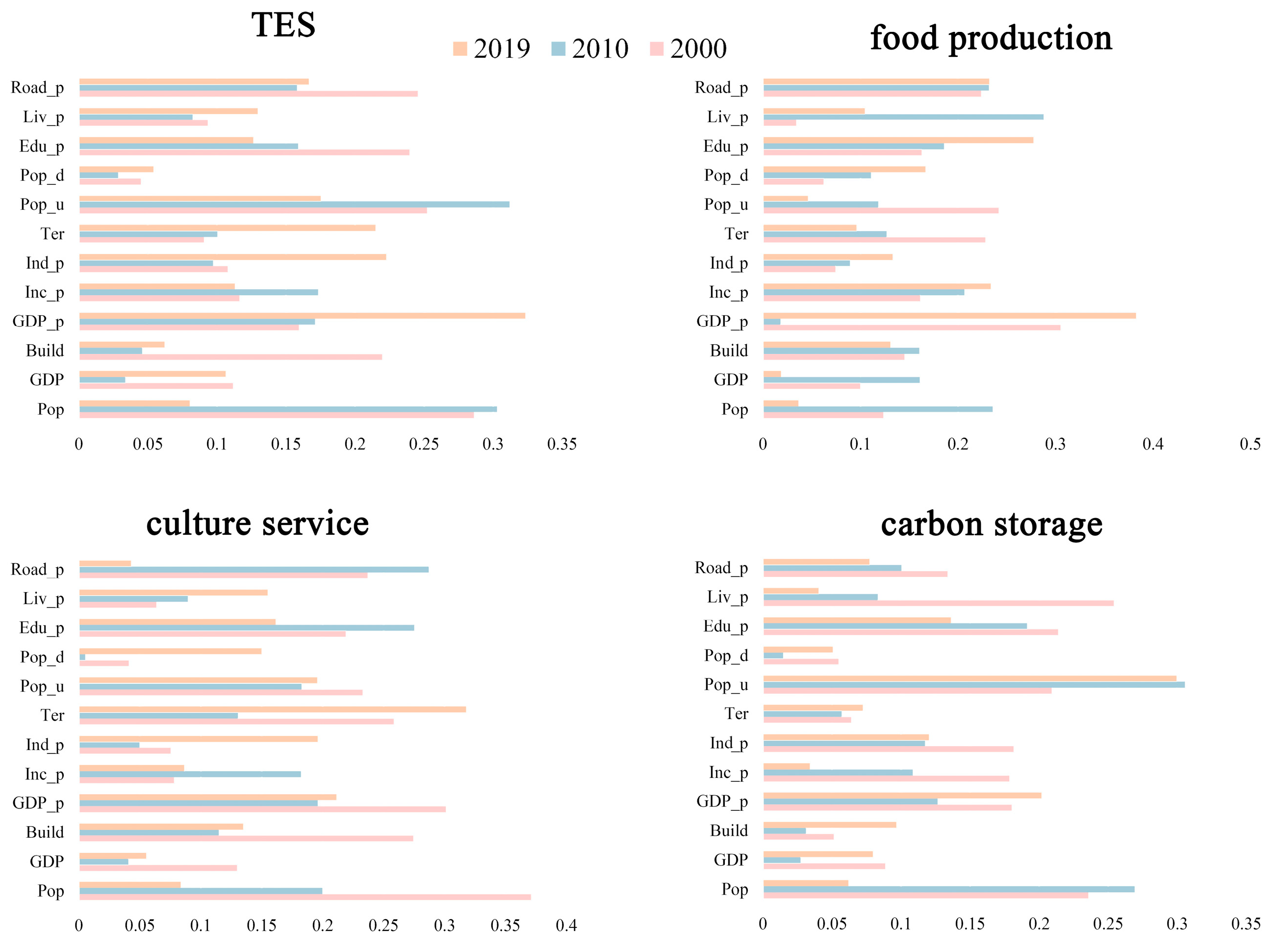

| Primary Indicator | Secondary Indicator | Unit | Abbreviation |
|---|---|---|---|
| Scale urbanization | Total population | 104 person | Pop |
| GDP | Million CNY | GDP | |
| Built up area | km2 | Build | |
| Economy urbanization | GDP per capita | 104 CNY | GDP_p |
| Per capita financial income | 104 CNY | Inc_p | |
| Per capita industrial output value | 104 CNY | Ind_p | |
| Proportion of tertiary industry | % | Ter | |
| Population urbanization | Population density in municipal districts | Person/km2 | Pop_d |
| Proportion of urban population | % | Pop_u | |
| Per capita expenditure on education | RMB | Edu_p | |
| Land urbanization | Per capita living area | m2 | Live_p |
| Per capita road area | m2 | Road_p |
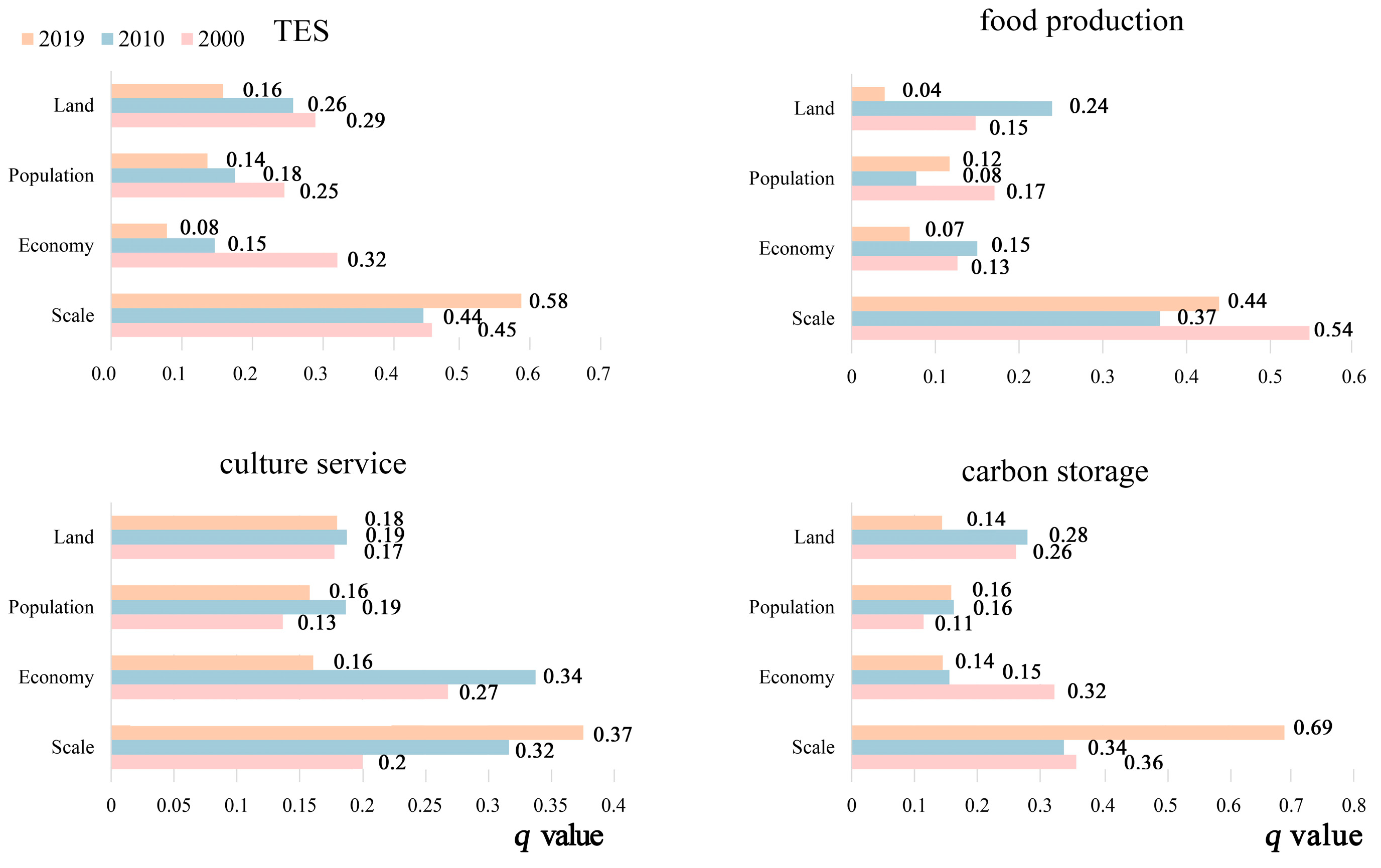
| ESs | Year | Scale Urbanization | Economy Urbanization | Population Urbanization | Land Urbanization |
|---|---|---|---|---|---|
| TES | 2000 | 0.32 | 0.36 | 0.11 | 0.66 |
| 2010 | 0.26 | 0.46 | 0.37 | 0.22 | |
| 2019 | 0.32 | 0.38 | 0.41 | 0.32 | |
| Food production | 2000 | 0.36 | 0.40 | 0.15 | 0.67 |
| 2010 | 0.26 | 0.30 | 0.30 | 0.17 | |
| 2019 | 0.31 | 0.26 | 0.41 | 0.31 | |
| Carbon storage | 2000 | 0.46 | 0.57 | 0.22 | 0.70 |
| 2010 | 0.27 | 0.45 | 0.42 | 0.20 | |
| 2019 | 0.38 | 0.36 | 0.37 | 0.41 | |
| Cultural service | 2000 | 0.32 | 0.44 | 0.16 | 0.68 |
| 2010 | 0.21 | 0.41 | 0.36 | 0.17 | |
| 2019 | 0.32 | 0.30 | 0.45 | 0.31 |
Disclaimer/Publisher’s Note: The statements, opinions and data contained in all publications are solely those of the individual author(s) and contributor(s) and not of MDPI and/or the editor(s). MDPI and/or the editor(s) disclaim responsibility for any injury to people or property resulting from any ideas, methods, instructions or products referred to in the content. |
© 2023 by the authors. Licensee MDPI, Basel, Switzerland. This article is an open access article distributed under the terms and conditions of the Creative Commons Attribution (CC BY) license (https://creativecommons.org/licenses/by/4.0/).
Share and Cite
Gong, J.; Dai, X.; Wang, L.; Niu, Z.; Cao, Q.; Huang, C. The Impact of Urbanization on the Supply–Demand Relationship of Ecosystem Services in the Yangtze River Middle Reaches Urban Agglomeration. Remote Sens. 2023, 15, 4749. https://doi.org/10.3390/rs15194749
Gong J, Dai X, Wang L, Niu Z, Cao Q, Huang C. The Impact of Urbanization on the Supply–Demand Relationship of Ecosystem Services in the Yangtze River Middle Reaches Urban Agglomeration. Remote Sensing. 2023; 15(19):4749. https://doi.org/10.3390/rs15194749
Chicago/Turabian StyleGong, Jie, Xin Dai, Lunche Wang, Zigeng Niu, Qian Cao, and Chunbo Huang. 2023. "The Impact of Urbanization on the Supply–Demand Relationship of Ecosystem Services in the Yangtze River Middle Reaches Urban Agglomeration" Remote Sensing 15, no. 19: 4749. https://doi.org/10.3390/rs15194749
APA StyleGong, J., Dai, X., Wang, L., Niu, Z., Cao, Q., & Huang, C. (2023). The Impact of Urbanization on the Supply–Demand Relationship of Ecosystem Services in the Yangtze River Middle Reaches Urban Agglomeration. Remote Sensing, 15(19), 4749. https://doi.org/10.3390/rs15194749