Abstract
3D reconstruction of urban scenes is an important research topic in remote sensing. Neural Radiance Fields (NeRFs) offer an efficient solution for both structure recovery and novel view synthesis. The realistic 3D urban models generated by NeRFs have potential future applications in simulation for autonomous driving, as well as in Augmented and Virtual Reality (AR/VR) experiences. Previous NeRF methods struggle with large-scale, urban environments. Due to the limited model capability of NeRF, directly applying them to urban environments may result in noticeable artifacts in synthesized images and inferior visual fidelity. To address this challenge, we propose a sparse voxel-based NeRF. First, our approach leverages LiDAR odometry to refine frame-by-frame LiDAR point cloud alignment and derive accurate initial camera pose through joint LiDAR-camera calibration. Second, we partition the space into sparse voxels and perform voxel interpolation based on 3D LiDAR point clouds, and then construct a voxel octree structure to disregard empty voxels during subsequent ray sampling in the NeRF, which can increase the rendering speed. Finally, the depth information provided by the 3D point cloud on each viewpoint image supervises our NeRF model, which is further optimized using a depth consistency loss function and a plane constraint loss function. In the real-world urban scenes, our method significantly reduces the training time to around an hour and enhances reconstruction quality with a PSNR improvement of 1–2 dB, outperforming other state-of-the-art NeRF models.
1. Introduction
The acceleration of urbanization leads to challenges in constructing intelligent/digital cities, which requires understanding and modeling of urban scenes. Over the past years, data-driven deep learning models have been widely adopted for scene understanding [1]. However, deep learning models are often hindered by domain gap [2,3] and heavily depend on a vast amount of annotated training data that is costly and complex to collect and label, particularly for the multi-sensor data annotation [4]. 3D reconstruction [5,6] can be used not only for data augmentation but also for direct 3D modeling of urban scenes [7]. Specifically, in the remote sensing mapping [8,9,10,11,12], it can generate high-precision digital surface models using multi-view satellite images [13,14] and combine the diversity of virtual environments with the richness of the real-world, generating more controllable and realistic data than simulation data.
With the emergence of Neural Radiance Fields (NeRF) [15], the research on 3D reconstruction algorithms has rapidly progressed [16]. Many researchers have applied the NeRF model to the field of remote sensing mapping [17,18]. Compared to classic 3D reconstruction methods with explicit geometric representations, NeRF’s neural implicit representation is smooth, continuous, differentiable, and capable of better handling complex lighting effects. It can render high-quality images from new perspectives based on the camera images and six degrees of freedom camera poses [19,20,21]. The core idea of NeRF is to represent the scene as a density and radiance field encoded by a multi-layer perceptron (MLP) network and train the MLP using differentiable volume rendering techniques. Although NeRF can achieve satisfactory rendering effects, the training of deep neural networks is time-consuming, i.e., in hours or days, which limits its application. Recent studies suggest that voxel grid-based methods, such as Plenoxels [22], NSVF [23], DVGO [24] and Instant-NGP [25], can rapidly train NeRF within few hours and reduce memory consumption through voxel cropping [23,24] and hash indexing [25]. Depth supervision-based methods such as DsNeRF [26] utilize the sparse 3D point cloud output from COLMAP [27] to guide NeRF’s scene geometry learning and accelerate convergence.
Although these methods demonstrate robust 3D reconstruction results in bounded scenes, when they are applied to urban unbounded scenarios, they confront several challenges. First, it is a common requirement to handle large-scale scenes with relatively fixed data collection. A NeRF representation requires spatial division of the 3D environment. Although NeRF++ [28] separates the scene into foreground and background networks for training, extending NeRF to unbounded scenes, the division of large-scale scenes requires more storage and computational resources and the algorithm would be difficult to use without optimization. Yet, the real outdoor scenario, such as urban environments, typically covers a large area in hundreds of square meters, which presents a significant challenge for NeRF representation. In addition, urban scene data are usually collected using cameras mounted on the ground or unmanned aerial vehicles without focusing on any specific part of the scene. Therefore, some scenes may be less observed or potentially missed by the cameras, while some other scenes may be captured multiple times from multiple viewpoints. Such uneven observation perspectives increase the difficulty of reconstruction [29,30].
Another challenge to NeRF methods is complex scenes with highly variable environments. A scene often contains a variety of target objects, such as buildings, signs, vehicles, vegetation, etc. These targets have significant differences in appearance, geometric shape, and occlusion relationships. The reconstruction of diverse targets is limited by model capacity, memory, and computation resources. Additionally, because cameras usually adopt automatic exposure, captured images often have high exposure variation, subject to the lighting condition. NeRF-W [31] addresses occlusions and lighting changes in the scene through transient object embedding and latent appearance modeling. However, its rendering quality drops for some areas, such as the ground, that are rarely included in training images, and blurriness often appears in scenes where the camera pose is incorrect. Thus, relying solely on image data faces the difficulties of camera pose estimation, leading to low-quality 3D reconstruction.
This problem can be relieved by using 3D LiDAR for pose inference and urban scene 3D geometric reconstruction [32,33,34,35], however, LiDAR point clouds also have inherent disadvantages. The point cloud resolution is usually low, and it is very difficult to generate point cloud data on glossy or transparent surfaces. For this issue, Google proposed Urban Radiance Fields in 2021 [36], which compensates for scene sparsity through LiDAR point clouds and supervises rays pointing to the sky through image segmentation, addressing the problem of light changes in the scene.
In this paper, the central aim is to develop a method that not only accelerates the process of reconstructing urban scenes but also improves the quality of 3D reconstruction. Therefore, different from Google’s solution, we propose to estimate accurate camera 6-DOF poses and 3D point cloud models through fine registration of LiDAR odometry output and per-frame LiDAR point clouds. Then, the space is divided into sparse voxels based on the prior of the 3D LiDAR point clouds, and a sparse voxel ray sampling method is designed to ignore empty voxels, so as to speed up training. Finally, depth consistency loss and local plane constraint loss are built based on the sparse point cloud, and the image is used for fine reconstruction. An overview of our method is outlined in Figure 1. The main contributions of this paper are summarized as follows:
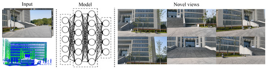
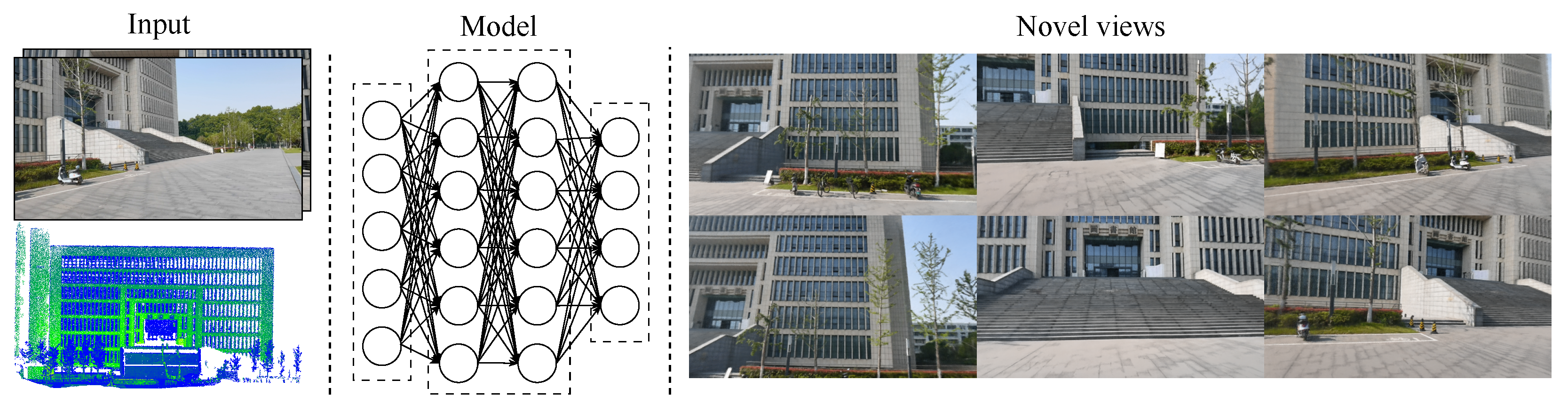
Figure 1.
Overview of Voxel-Based Neural Radiance Field 3D Reconstruction. The input comprises images, corresponding camera pose, and LiDAR point cloud priors. Model is constructed based on a MLP framework. The output includes the results of 3D reconstruction and novel view synthesis.
- We can obtain accurate initial camera pose and a priori 3D point cloud models through LiDAR odometry and LiDAR-camera calibration, which can reduce the artifacts in synthesizing novel views and enhance the reconstruction quality.
- We propose a novel NeRF 3D reconstruction algorithm that employs sparse voxel partitioning. By dividing space into sparse voxels and constructing a voxel octree structure, we can accelerate 3D reconstruction for urban scenes and enhance scene geometric consistency.
- Experimental results on four urban outdoor datasets indicate that our method can reduce the training time and significantly improve 3D reconstruction quality compared with the latest NeRF methods.
The remainder of this paper is outlined as follows. Section 2 compares the differences between classic 3D reconstruction methods and NeRF, and discusses the application of NeRF in urban scenes modelling. Section 3 introduces the sparse voxel-based neural radiance field and the optimization strategies. Section 4 analyses the results through the urban scene datasets, and Section 5 concludes this paper and describes future work.
2. Related Works
In this section, we introduce classic 3D reconstruction and NeRF and discuss the recent advance and applications of NeRF methods in urban scenes.
2.1. Classic Methods of 3D Reconstruction
Classic 3D reconstruction methods initially collate data into explicit 3D scene representations, such as textured meshes [37] or primitive shapes [38]. Although effective for large diffuse surfaces, these methods can not well handle urban scenes due to the complexity of geometric structures. Alternative methods use 3D volumetric representations such as voxels [39], octrees [40], but their resolution is limited, and their storage demands for discrete volume are high.
For large-scale urban scenes, Li proposed AADS [41] to utilize images and LiDAR point clouds for reconstruction, amalgamating perceptual algorithms and manual annotation to formulate a 3D point cloud representation of moving foreground objects. In contrast, SurfelGAN [42] employed Surfels for 3D modeling, capturing 3D semantic and appearance information of all scene objects. These methods rely on explicit 3D reconstruction algorithms like SfM [43] and MVS [44], which recover dense 3D point clouds from multi-view imagery [45]. However, the resulting 3D models often contain artifacts and holes in weakly textured or specular regions, requiring further processing for novel view image synthesis. While these methods focus on reconstruction accuracy, our research seeks not only to ensure high-precision 3D reconstruction but also to reduce the associated training time.
2.2. Neural Radiance Fields
2.2.1. Theory of Neural Radiance Fields
Neural rendering techniques, exemplified by Neural Radiance Fields (NeRF) [15], allow neural networks to implicitly learn static 3D scenes from a series of 2D images. Once the network has been trained, it can render 2D images from any viewpoint. More specifically, Multilayer Perceptron (MLP) is employed to represent the scene. The MLP takes a 3D positional vector of a spatial point and a 2D viewing direction vector as inputs and maps them to the density and color vector of that location. Subsequently, a differentiable volume rendering method [46] is used to synthesize any new view. Typically, this representation is trained within a specific scene. For a set of input camera images and poses, the NeRF employs gradient descent to fit the function by minimizing the color error between the rendered results and the real images.
2.2.2. Advance in NeRF
Many research [47,48,49,50,51,52,53,54] have augmented the original NeRF, enhancing reconstruction accuracy, rendering efficiency, and generalization performance. MetaNeRF [55] improved accuracy by leveraging data-driven prior training scenes to supplement missing information in test scenes. NeRFactor [56] employed MLP-based factorization to extract information on illumination, object surface normals and light fields. Barron et al. [57] substitute a view cone for line-of-sight perception, minimizing jagged artifacts and blur. Addressing NeRF’s oversampling of blank space, Liu et al. [23] proposed a sparse voxel octree structure for 3D modeling. Plenoxels [22] bypassed extensive MLP models to predict density and color and instead stored these values directly on the voxel grid. Instant-NGP [25] and DVGO [24] constructed feature meshes and densities, calculating point-specific densities and colors from interpolated feature vectors using compact MLP networks.
To improve the model’s generalizability, Yu et al. [20] introduced PixelNeRF, allowing the model to perform view synthesis tasks with minimal input by integrating spatial image features at the pixel level. Our work concentrates on the challenges associated with urban outdoor environments and low rendering efficiency. Recently, Martin-Brualla et al. [31] conducted a 3D reconstruction of various outdoor landmark structures utilizing data sourced from the Internet. DS-NeRF [26] reconstructed sparse 3D point clouds from COLMAP [27], using inherent depth information to supervise the NeRF objective function, thereby enhancing the convergence of scene geometry.
2.3. Application of NeRF in Urban Scene
Some researchers have applied NeRF to urban scenes. Zhang et al. [28] addressed parameterization challenges in extensive, unbounded 3D scenes by dichotomizing the scene into foreground and background with sphere inversion. Google’s Urban Radiance Field [36] used LiDAR data to counteract scene sparsity and employed an affine color estimation for each camera to automatically compensate for variable exposures. Block-NeRF [58] broke down city-scale scenes into individually trained neural radiance fields, uncoupling rendering time from scene size. Moreover, City-NeRF [59] evolved the network model and training set concurrently, incorporating new training blocks during training to facilitate multi-scale rendering from satellite to ground-level imagery.
Although these methods focus on 3D reconstruction precision, they require extended model training times. In this paper, we integrate LiDAR point cloud data to segment the space, and build the sparse voxel octree structure, finally perform 3D reconstruction of urban scenes based on accurate camera pose and images. Our method enhances the performance and computational efficiency of the 3D reconstruction model, further broadening the application of neural radiance fields in urban outdoor environments.
3. Methodology
In this section, we first introduce the fundamental theory of NeRF, then give a detailed elaboration on the construction scheme and training optimization strategies of Sparse Voxel-based NeRF, as shown in Figure 2.

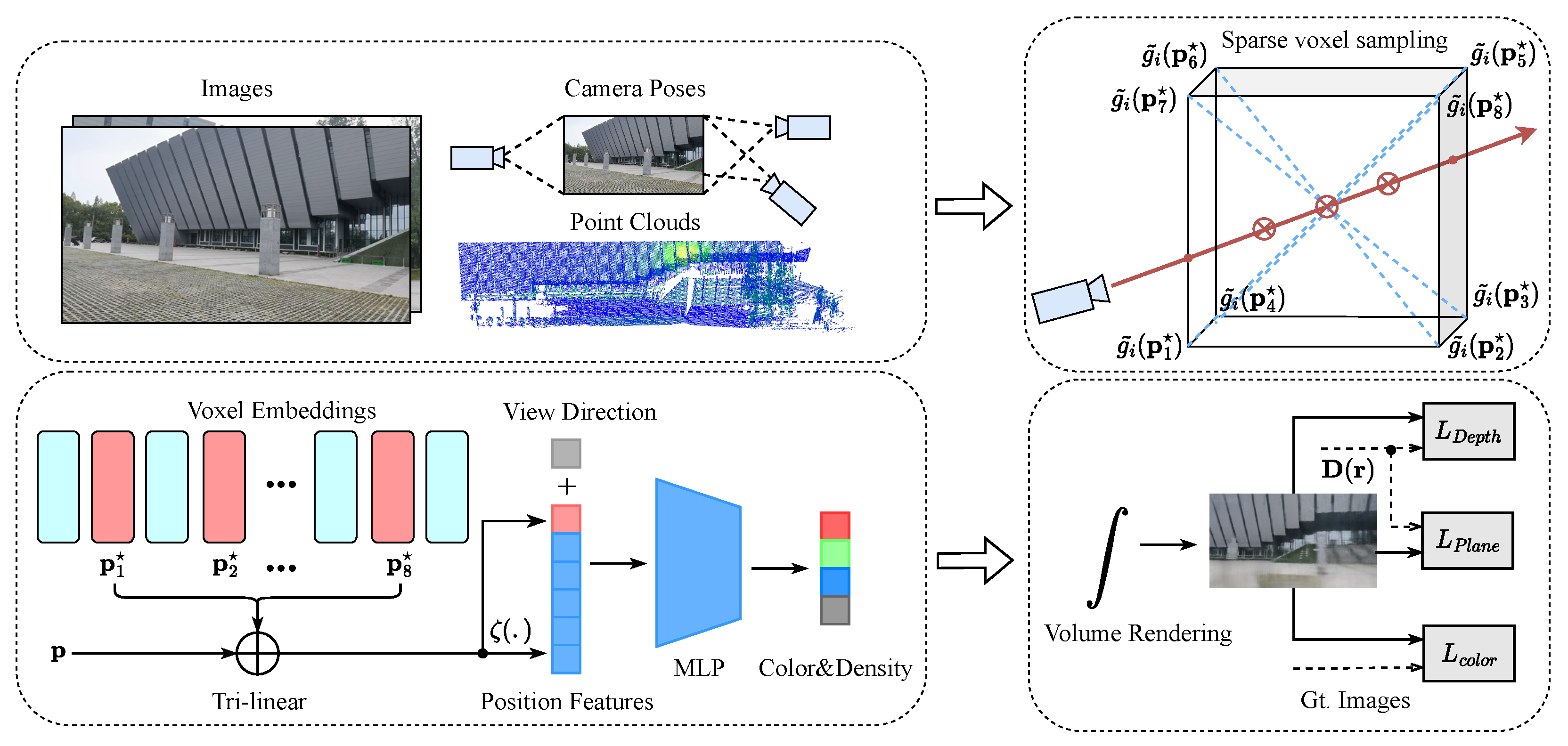
Figure 2.
Pipeline of Voxel-Based Neural Radiance Field 3D Reconstruction. We use camera images, the corresponding camera poses, and LiDAR point clouds as the input to construct a sparse voxel set. Upon sparse voxel sampling, the voxel embedding is queried and interpolated to yield a feature representation based on eight corresponding voxel vertices. Finally, the MLP is trained and optimized based on the results of volume rendering. More details about the model architecture can be found in Appendix A.
3.1. Preliminaries
NeRF aims to simulteneously accomplish 3D reconstruction and synthesis of novel viewpoints. NeRF represents a set of continuous scene images with known camera pose as an implicit field function . The inputs include a three-dimensional position vector and a two-dimensional viewpoint direction vector . The outputs are the voxel density at that position and a color vector related to the viewpoint .
NeRF first uses a high-frequency mapping function to map the three-dimensional point coordinate and direction vector to a high-dimensional space using the following Equation (1):
where represents the input of the function, and L indicates the dimensional information in the high-frequency space. For coordinate encoding, , while for direction encoding, . Coordinate encoding is used as the input into MLP to obtain and intermediate features , which, in combination with , are fed into additional fully connected layers to predict the color as follows:
Here, the density is a function related to spatial position , while color is a function of both spatial position and viewing direction . Consequently, when the same location is observed from different angles, the color will change according to the viewpoint. To ensure that the network can be trained, density and color obtained from NeRF use a differentiable rendering method. For a ray emanating from the camera center , the color value of any pixel it passes through is obtained by the following integral:
where represents the cumulative transparency along the ray in direction t. The model is optimized by the color consistency loss function using a gradient descent method:
where represents a given camera viewpoint. By computing the projection of each rays from this viewpoint, the image can be rendered for that viewpoint. The color consistency loss minimizes the per-pixel difference between the rendered result and the ground truth image .
3.2. Sparse Voxel NeRF Representation
Assuming the non-empty parts of the scene are contained in a set of sparse voxels, we divide the space into a collection of sparse voxels, , based on point clouds. The implicit field function can then be represented as , where denotes the point position information within the voxel. The implicit field function is represented by an MLP with shared weights :
where and represent the color and density of point respectively, and denotes the position encoding at point :
Here, are the 8 vertices of the voxel set , and are the feature vectors stored at all vertices. Additionally, is a trilinear interpolation, and is a post-processing function. In our experiments, is the positional encoding proposed in NeRF, as shown in Equation (1).
Trilinear interpolation notably outperforms simple nearest-neighbor interpolation. The benefits of interpolation are twofold. First, it can enhance the resolution by representing sub-voxel variations of color and density. Second, continuity induced by interpolation is crucial for the optimization process. While most previous works employ the 3D coordinates of point as the input to , we use the feature vector aggregated from the embeddings of the corresponding 8 voxels. These voxels can embed information specific to particular regions, such as geometry and color. This approach significantly simplifies the learning of the subsequent implicit field function and promotes high-quality rendering.
Sparse Voxel Sampling Method
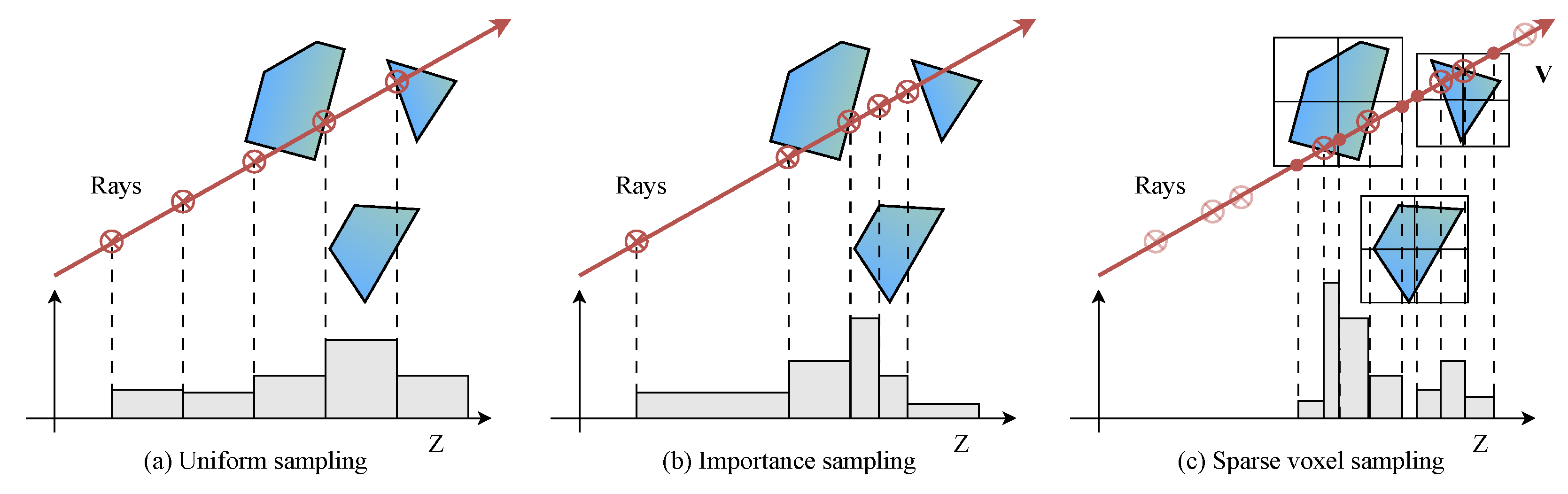
As illustrated in Figure 3, naive sampling methods waste computational resources in sampling spaces not covered by effective voxels, like the hierarchical random sampling employed by the original NeRF. Therefore, we propose a sparse voxel sampling method inspired by NSVF [23]. An AABB intersection test [60] is initially conducted on all sampling pixels to ascertain voxel-ray intersections and any pixel with no hits is masked out. Given that urban outdoor environments are unbounded, we set a parameter that one single pixel can see the maximal number of voxels. Unlike the original NSVF, where the parameter is set according to empirical values, we dynamically adjust it based on a specified maximum sampling distance .
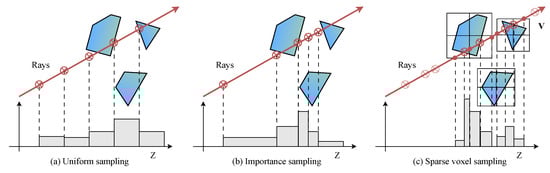
Figure 3.
Visual Demonstration of Ray Sampling Methods: Compared to the prior two ray sampling methods, sparse voxel sampling offers superior computational efficiency by eliminating sampling points within empty spaces.
3.3. Optimization
3.3.1. Multi-Sensor Fusion
The platform to collect outdoor large-scale images and 3D point cloud data consists of a Livox Avia LiDAR and an OAK-D-Pro camera. They have been time-synchronized and spatially aligned. In Figure 4, we employ LiDAR odometry and LiDAR-camera calibration to refine the 3D point cloud model and obtain the accurate camera pose.
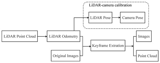
Figure 4.
The illustration of the data preprocessing. We employ LiDAR-camera calibration to get accurate camera pose. Through keyframe extraction, we are able to obtain image data and 3D point cloud, which has been optimized from LiDAR odometry.
For the LiDAR point cloud registration and camera pose optimization step, an improved LiDAR odometry approach based on Lego-LOAM [61] is adopted to perform refined scan-to-map matching for frame-by-frame LiDAR point clouds. We incorporate IMU pre-integration to eliminate motion distortion in the point cloud. Considering that our primary focus is 3D reconstruction of static urban scenes, we integrate a dynamic object processing feature in the odometry. This aids in filtering out ghost points caused by dynamic objects in the scene, thereby enhancing the accuracy of the 3D point cloud model.
In the LiDAR and camera extrinsic calibration step, following the sensor calibration scheme proposed by Yuan [62] and the LiDAR pose output from the LiDAR odometry, we obtain a precise initial camera pose corresponding to the images, which serves as the input to the sparse voxel-based neural radiance field.
3.3.2. Self-Pruning
We first learn an implicit function for a set of initial voxels, roughly bounding the scene. In this paper, LiDAR point clouds are used for initialization, with the voxel size set to . We implement a self-pruning strategy for coarse geometric information based on NSVF. This can effectively remove unnecessary voxels during the training process. A voxel needs to be pruned when the following conditions are met:
where represents G uniformly sampled points in the ray direction within voxel , predicts the voxel density at point , and is a threshold set to in our experiments. Periodically self-pruning voxels after the appearance of coarse scene geometry can gradually adjust voxelization to adapt to the underlying scene structure.
In our experiments, we train real urban outdoor scenes in three stages. Specifically, we first initialize the ray marching step size and voxel size for training optimization. After a certain number of iterative training steps, the step size and voxel size for the next phase are halved, effectively subdividing all voxels into sub-voxels and initializing the feature representation of the new vertices. Essentially, we gradually increase the model’s capability to understand more scene details.
3.3.3. Loss Function
The optimization loss is composed of three parts: color consistency loss , sparse point cloud depth loss , and local plane constraint loss :
where and are weight hyperparameters and is given by Equation (4). The sparse point cloud depth is similar to the image rendering process in Equation (3). Given a viewpoint ray , the depth rendering from near end to far end can be expressed as:
Given the camera viewpoint and loss function in Equation (8), we calculate the rendered depth of the ray set with existing LiDAR point cloud data from this viewpoint. The sparse point cloud depth loss function minimizes the difference between this rendered depth and the actual depth :
To enhance the structural constraints of the 3D model, this paper introduces the slanted plane model into the NeRF training framework. It assumes that all pixels within a superpixel are located on the same 3D plane. Specifically, we define the set of all pixel positions within a superpixel as matrix , represented in homogeneous coordinates. The set of all depth values is and the identity matrix is represented as . The local plane constraint loss is to minimize the distance sum of all points to this plane as follows:
4. Experiments
In this section, we demonstrate a series of experiments on self-collected urban outdoor scene datasets to evaluate our proposed model. The experiments are used to assess whether the proposed algorithm can improve the efficiency of training and render more accurately.
4.1. Experimental Settings
4.1.1. Dataset and Metrics
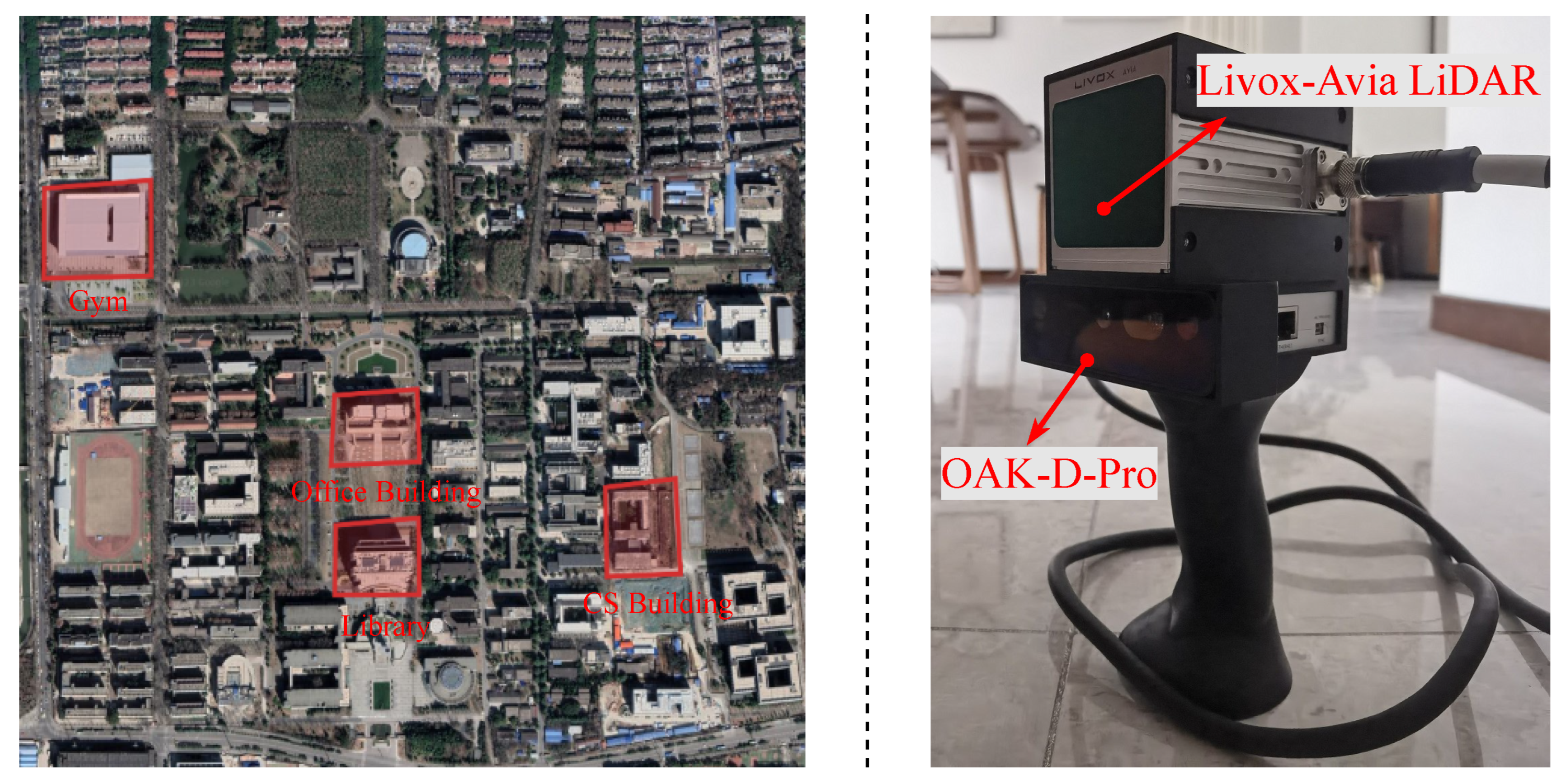
Our sensor platform is equipped with Livox Avia LiDAR and OAK-D-Pro camera as shown in Figure 5, and was designed for handheld data collection. The datasets comprise four urban scenes, which are named as a landmark: Gym, Office Building, CS Building, and Library. For each scene, approximately 300 images and 100 LiDAR point cloud frames were collected. More details about the datasets can be found in Appendix B. After refined registration using LiDAR odometry, key frames were identified through traditional feature extraction and matching, generating 50 images and corresponding downscaled 800,000 LiDAR points. Each scene includes a free camera trajectory and multiple focused foreground objects, posing a significant challenge to the 3D reconstruction.

Figure 5.
The left satellite image illustrates the location of our data collection. The right image shows our handheld multi-sensor platform, which includes a Livox Avia LiDAR and an OAK-D-Pro camera.
To evaluate our method, given an image with a camera pose, we render and compare it with the ground truth. Evaluation metrics are based on PSNR, SSIM, and LPIPS [63]. PSNR is a standard measure for image quality assessment, gauging the difference between the original image and the rendered image. A higher PSNR value indicates the better quality of the reconstructed image. SSIM is another index used to assess the similarity between two images, which pays more attention to the structure and texture information of the image. If SSIM is closer to 1, it signifies the higher similarity between two images. LPIPS is a perceptual image similarity metric based on deep learning, it trains a neural network model to learn the sensitivity of human eyes to image differences, so as to measure the perceptual differences between two images. The smaller the value, the more similar the two images are perceptually.
4.1.2. Baseline Methods
We compare our method with the state-of-the-art NeRF-like methods as shown in Table 1. Except for NeRF, other methods can handle unbounded scenes. DVGO and Plenoxels are voxel-based methods. Only DSNeRF and our method use depth supervision. DSNeRF uses 3D sparse point clouds obtained from COLMAP, while our method constructs a sparse voxel NeRF using point clouds gathered by LiDAR.

Table 1.
Comparison of 3D reconstruction methods for NeRF. Unbouded means.
4.1.3. Implementation Details
We implemented an octree structure for voxels and set the learned feature vector of voxel vertices to 32 dimensions. The overall network architecture in Figure 2 was implemented in Pytorch. Following the general NeRF setup, one image was set as the test image out of every five images, the rest forming the training set. Training was conducted on a single Nvidia-V100-32 GB, with 2048 rays sampled from all images and only rays that hit at least one voxel were sampled.
4.2. Result Analysis
As demonstrated in Table 2 and Table 3, we conduct quantitative comparisons on four urban scene datasets. The original NeRF model struggles with unbounded scenes, yielding poorer reconstruction and longer training times than other methods. Both DVGO and Plenoxels, which are voxel-based methods, achieve fast convergence within 40 min due to their voxel ray sampling strategy, but the reconstruction quality lags behind our method. NeRF++ trains foreground and background separately and achieves similar reconstruction quality as ours but suffers from low computational efficiency—it takes two days for training. Through accurate initial camera pose, 3D point cloud priors, and loss functions designed in this paper, our model outperforms all recent NeRF-like models, and achieves the highest quality for view synthesis with the improvement of 4– over the baseline, while converging time is around an hour. Specifically, we observe the PSNR increase to around 30 dB, the SSIM improvement to approximately 0.9, and a decrease in LPIPS to about 0.2, underlining the accuracy and precision of our reconstruction method.
Table 2.
Comparison of NeRF 3D Reconstruction Results on Gym and Office Building Datasets.
Table 3.
Comparison of NeRF 3D Reconstruction Results on CS Building and Library Datasets.
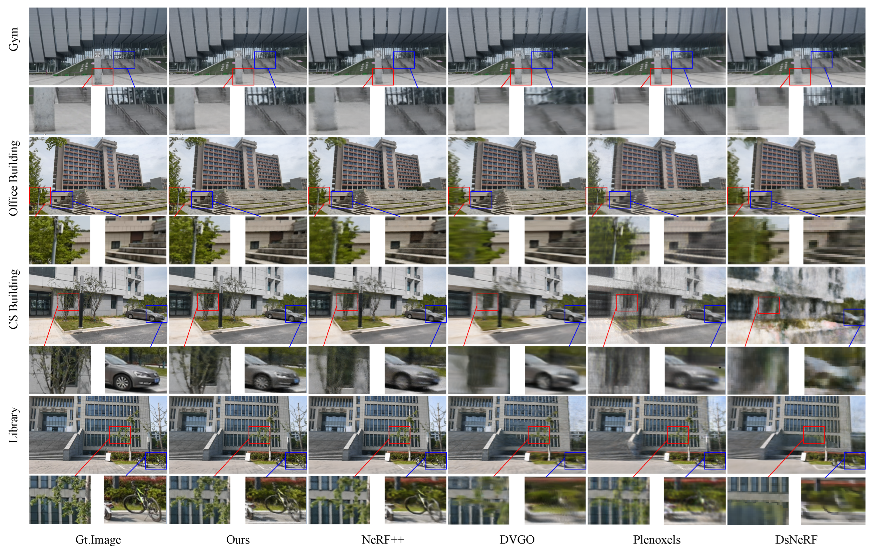
Figure 6 presents the qualitative comparison of the rendered scenes. Given the variability of perspectives in the scene, DsNeRF yields blurry reconstruction details due to the imprecise camera pose and sparse 3D point cloud obtained from COLMAP. DVGO and Plenoxels, although employing voxel methods, produce blurry synthesized images due to limited resolution, incapable of representing arbitrary camera pose trajectories. While NeRF++ offers clearer results, it still lags behind our method in scene details, such as nearby vegetation and distant vehicles. Our method utilizes the point cloud prior for depth supervision, enhancing the precision of the scene’s geometric structure. The camera poses, derived from LiDAR odometry and LiDAR-camera extrinsic calibration, support unrestricted long trajectories, accommodating perspective shifts inherent, such as in urban scenes.
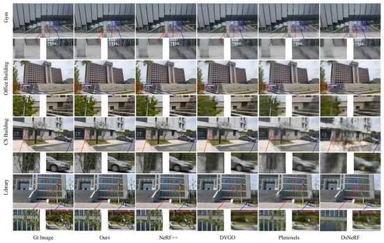
Figure 6.
Visual comparison on the four outdoor scene datasets.
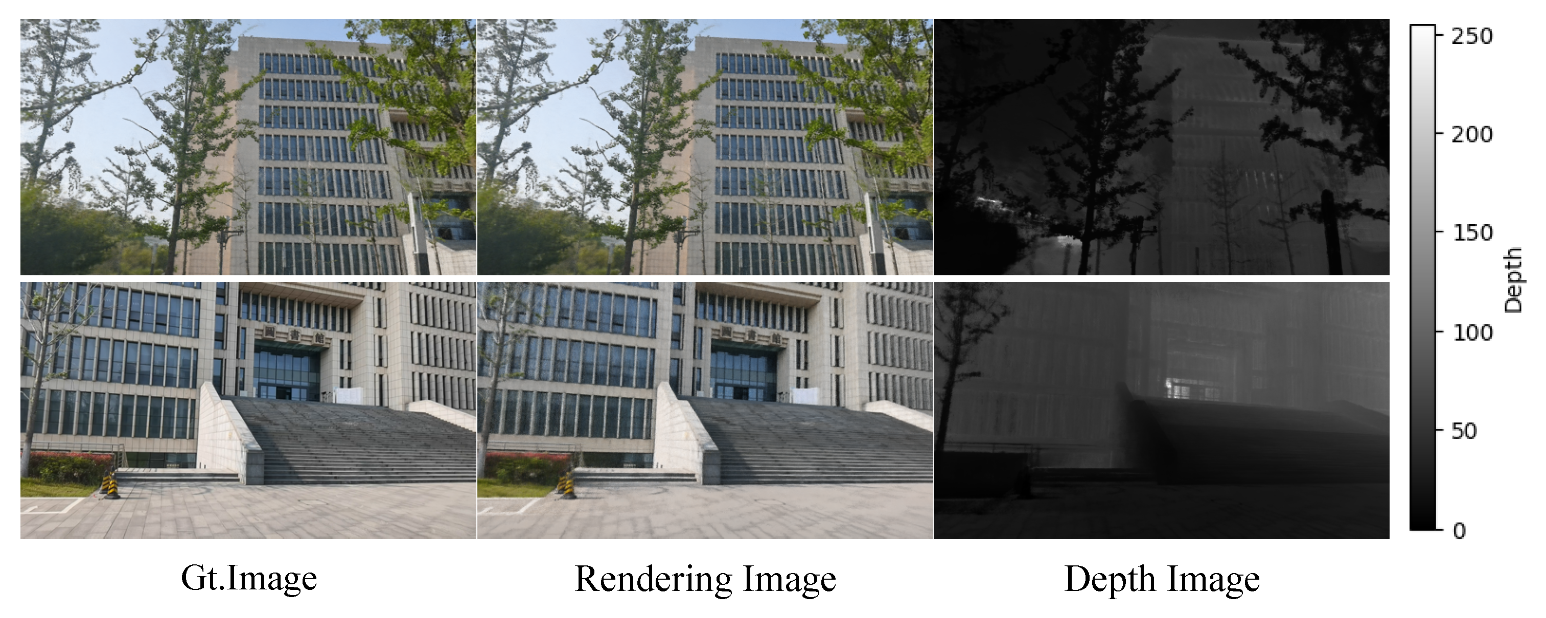
In Figure 7, the depth maps of rendered images in the scene dataset are visualized. The vegetation, steps, and library buildings in the scene exhibit clear depth distinctions. By utilizing depth loss supervision, the rendering quality can be improved, particularly for scenes with a hierarchical depth structure.
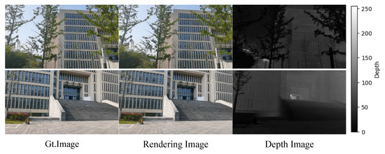
Figure 7.
Depth image visualization on Library datasets.
In our method, the voxel size is set to based on empirical values. As shown in Table 4, we conducted the experiments to compare the performance with voxel sizes of , , , and . The smaller the voxel size, the finer the representation of scene space details, thus improving the quality of rendered images. However, it also increases computational complexity and prolongs the model training time. As the voxel size is set smaller, the improvement in image rendering quality tends to saturate. Therefore, is chosen as the suitable empirical voxel size for 3D reconstruction using the NeRF.
Table 4.
Result analysis of voxel size on Library Datasets.
4.3. Ablation Studies
To fully validate the effectiveness of our 3D reconstruction algorithm based on sparse voxel NeRF, we conducted ablation experiments on the trained loss function and image resolution using the Library datasets.
As shown in Table 5, on the Library dataset, the rendering quality drops significantly when only using the color consistency loss. The local plane constraint is targeted at the 3D planar structure of scene reconstruction, and such constraint is helpful to improve the quality of rendering. With the addition of depth supervision from the sparse point cloud, the synthesis effect of novel views is significantly improved, which suggests that depth prior information can effectively guide the model to learn the geometric structure of the scene and carry out precise 3D reconstruction.
Table 5.
Ablation Study of Loss Functions on Library Datasets.
In Section 4.2, we employ 720 p image resolution, a LiDAR detection range of 400 m, and a maximum camera FOV of for our experiments. Table 6 elucidates the impact of varying image resolutions on the quality of reconstructions, supplemented by NIQE evaluation metrics. Although an uptrend in image resolution results in marginal improvements in reconstruction quality, the gains are modest. Future work could focus on nuanced analyses tailored to the specific attributes of high-resolution imagery.
Table 6.
Ablation Study of Image Resolution on Library Datasets.
5. Conclusions
This paper introduces a novel method for the 3D reconstruction of neural radiance fields based on sparse voxels with the aid of LiDAR point cloud prior, which can accomplish the 3D reconstruction of urban outdoor environments. Specifically, the paper first delineates the existing issues of the original neural radiance fields, including slow convergence speed during training and mainly focusing on small object reconstruction and the inapplicability of rendering for urban scenes. Subsequently, we propose a method for acquiring initial camera pose values based on the positional information output from LiDAR odometry and LiDAR-camera calibration, which allows for a frame-by-frame refined registration of the point cloud to procure a 3D point cloud model. Our method uses the point cloud prior for voxelization and space partitioning, then combines it with the image for the scene reconstruction. Experimental results demonstrate that our algorithm not only accelerates the convergence speed of neural radiance field training to approximately one hour but also enhances the quality of scene reconstruction by 4– compared with recent neural radiance field methods.
However, in the data acquisition part, considering the large-scale features of urban scenes, the processing time for 3D point cloud models and images increases with the expansion of the scene area. Therefore, optimizations can be made to the LiDAR odometry algorithms and adjustments to the downsampling parameters to reduce data acquisition time. Our algorithm also has its limitations. It is primarily focused on the 3D reconstruction of static urban scenes and struggles with dynamic foreground elements like moving vehicles or walking pedestrians. Moreover, due to the sensitivity of sensors to weather conditions such as smog and rainfall, the quality of reconstruction is adversely affected. Therefore, we plan to extend the NeRF algorithm in the future. By freely combining multi-object models and controlling implicit encoding of environmental factors, we can generate image synthesis with new perspectives and targets. We can also extend this capability to reconstruct moving underwater objects through the introduction of learnable medium parameters, which mitigate the interference between the camera and the scene. Furthermore, we will integrate denoising and restoration techniques into the preprocessing steps to better cope with complex weather conditions. We hope the research will pave the way for further enhancements in the domain of urban scene reconstruction and further leverage it for Augmented/Virtual Reality (AR/VR) applications.
Author Contributions
X.C. conceptualized the study, performed data processing, methodology development, and wrote the original draft. Z.S. conceptualized the study and writing. J.Z. reviewed and edited the manuscript. D.X. contributed to data processing. J.L. provided project administration and supervision. All authors have read and agreed to the published version of the manuscript.
Funding
This work was supported by the National Natural Science Foundation of China (Grant No. 62221004).
Data Availability Statement
The data that support the findings of this research are available from the corresponding author upon reasonable request.
Acknowledgments
The authors would like to thank the people who share the algorithm of LiDAR odometry and basic NeRF models of their research with the community and acknowledge all the teachers for the suggestions that helped improve the quality of this paper. This paper was carried out in part using computing resources at the High-Performance Computing Platform of Nanjing University of Science and Technology.
Conflicts of Interest
The authors declare no conflict of interest.
Appendix A. Model Architecture Details
In our algorithms, a 32-dimensional learnable voxel embedding is first assigned to each voxel vertex, and undergoes positional encoding with a maximum frequency of . The features, aggregated from voxel embeddings of eight vertices, are then trilinearly interpolated. Figure A1 presents the structure of the MLP, we simplified based on the NSVF [23]. The resulting feature representation and view direction vector are fed into a hidden layer of width 128 to obtain the scene features and volume density. The scene features and view direction vector are then jointly fed into another MLP comprising three hidden layers, each with a width of 128, to get the RGB color. The number of parameters for the entire model is less than 0.5 M.
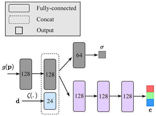
Figure A1.
A visualization of the voxel-based MLP architecture.
Figure A1.
A visualization of the voxel-based MLP architecture.

Appendix B. Datasets
As shown in Figure A2, we independently collected urban scene datasets using the Livox Avia LiDAR and OAK-D-Pro camera, which includes four scenarios: Gym, Office Building, CS Building and Library. Table A1 presents the specs on Livox Avia LiDAR and OAK-D-Pro camera. Each scenario includes 3D point cloud priors, images, LiDAR-camera extrinsics, and LiDAR trajectory poses. The 3D point cloud priors are obtained through LiDAR odometry, which are cropped and manually denoised after accumulating multiple frames, extracting keyframes and voxel downsampling. The images have a resolution of 1920 × 1080 without further processing. The camera pose can be obtained through the LiDAR-camera extrinsics from calibration and the LiDAR trajectory poses from LiDAR odometry. In Figure A3, We show the scenarios of LiDAR-camera calibration along with the corresponding visualization results.
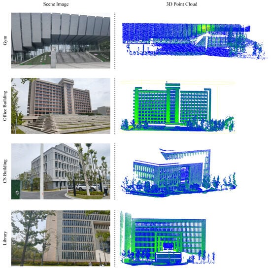
Figure A2.
The left image illustrates the four urban scene datasets which we collected. The right image shows the result of 3D point cloud priors.
Figure A2.
The left image illustrates the four urban scene datasets which we collected. The right image shows the result of 3D point cloud priors.
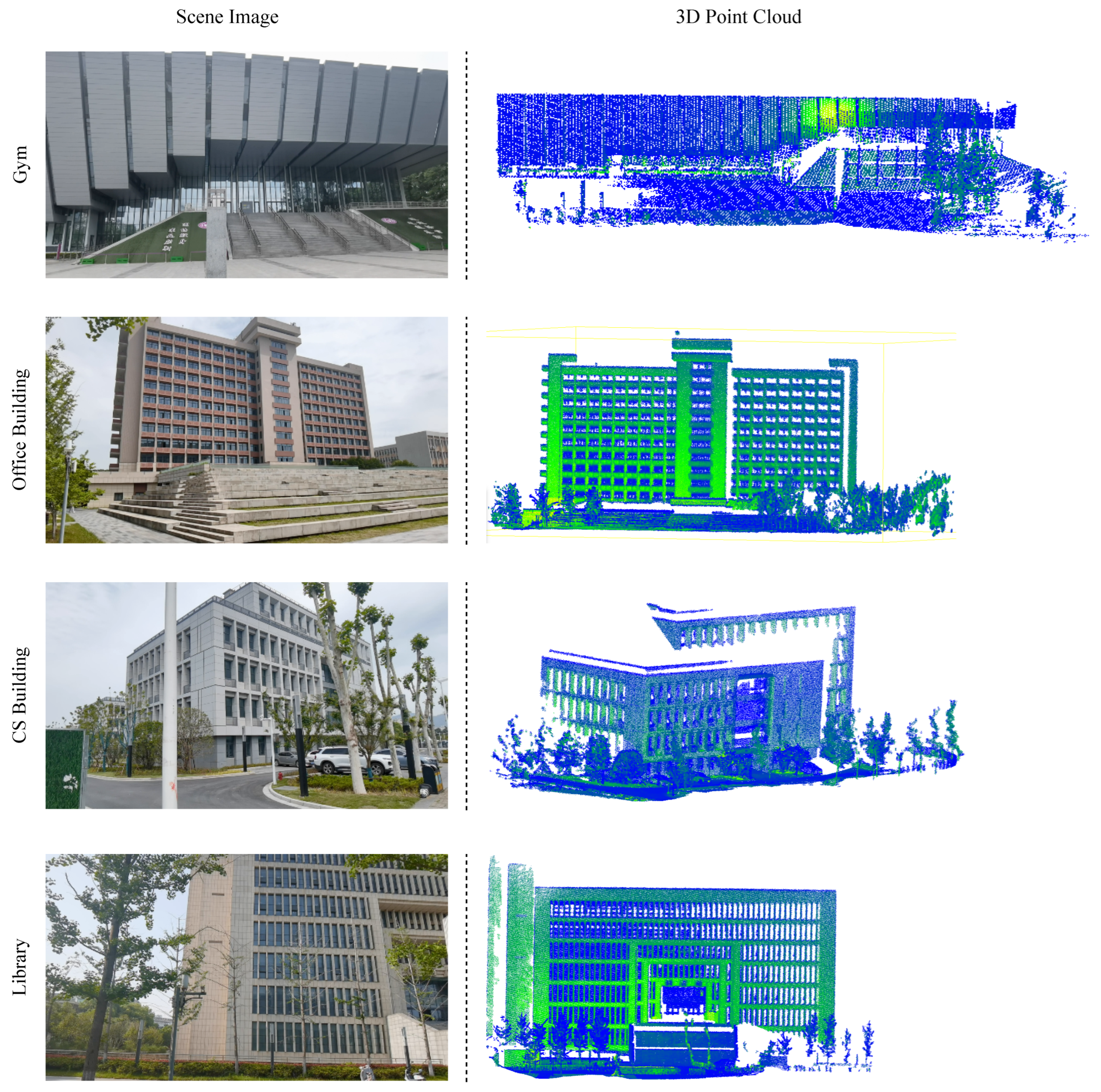
Table A1.
Descriptions of the specs on Livox Avia LiDAR and OAK-D-Pro Camera.
Table A1.
Descriptions of the specs on Livox Avia LiDAR and OAK-D-Pro Camera.
| Livox Avia LiDAR | OAK-D-Pro Camera | ||
|---|---|---|---|
| Parameter | Value | Parameter | Value |
| Laser Wavelength | 905 nm | Image Sensor | Sony IMX378 |
| Angular Precision | <0.05° | Active Pixels | 12 MP@60 fps |
| Range Precision | 2 cm1 | EFL | 4.81 |
| Data Latency | ≤2 ms | Focous Type | AF: 8 cm–∞/FF: 50 cm–∞ |
| HFOV/VFOV | 70.4°/77.2° | DFOV/HFOV/VFOV | 81°/69°/55° |
| Noise | <45 dBA | F.NO | 2.0 |
| Weight | 498 g | Shutter Type | Rolling shutter |
| IMU | Built-in: BMI088 | IR Sensitive | No |
Note: The range precision of 2 cm1 refers to the standard deviation (1) of the ranging error at a distance of 20 m.
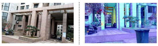
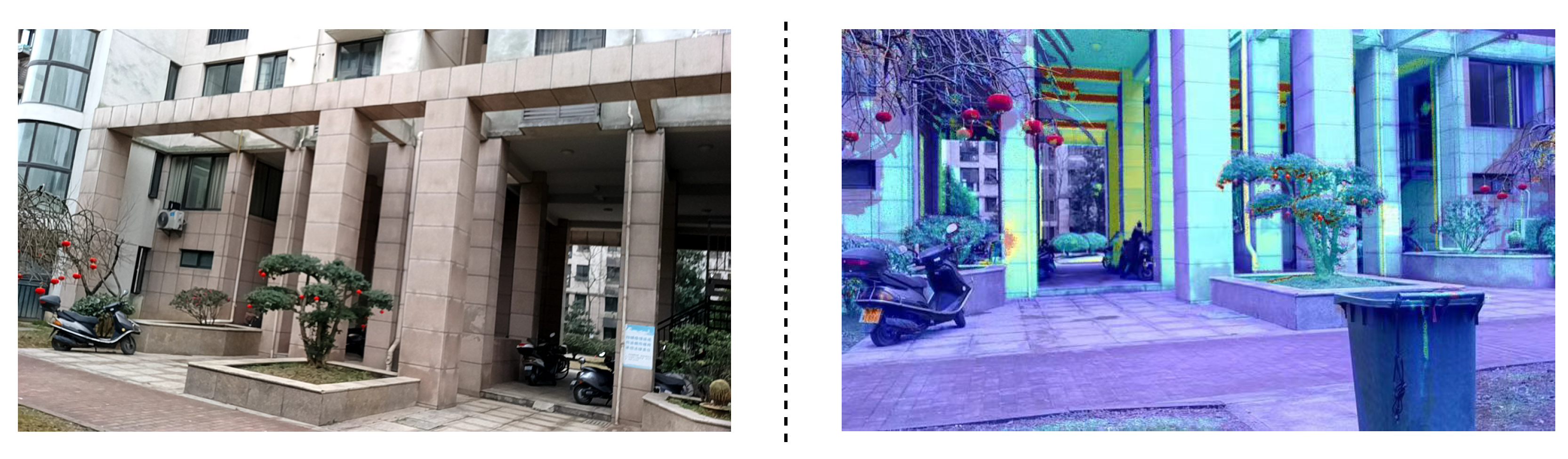
Figure A3.
The left image illustrates the scene used for LiDAR-camera calibration. The right image shows the result of projecting the LiDAR point cloud onto the image using extrinsics between LiDAR and camera.
Figure A3.
The left image illustrates the scene used for LiDAR-camera calibration. The right image shows the result of projecting the LiDAR point cloud onto the image using extrinsics between LiDAR and camera.
References
- Xu, R.; Xiang, H.; Tu, Z.; Xia, X.; Yang, M.H.; Ma, J. V2x-vit: Vehicle-to-everything cooperative perception with vision transformer. In Proceedings of the European Conference on Computer Vision, Tel Aviv, Israel, 23–28 August 2022; Springer: Berlin/Heidelberg, Germany, 2022; pp. 107–124. [Google Scholar]
- Xu, R.; Li, J.; Dong, X.; Yu, H.; Ma, J. Bridging the domain gap for multi-agent perception. In Proceedings of the 2023 IEEE International Conference on Robotics and Automation (ICRA), London, UK, 29 May–2 June 2023; pp. 6035–6042. [Google Scholar]
- Xu, R.; Chen, W.; Xiang, H.; Xia, X.; Liu, L.; Ma, J. Model-agnostic multi-agent perception framework. In Proceedings of the 2023 IEEE International Conference on Robotics and Automation (ICRA), London, UK, 29 May–2 June 2023; pp. 1471–1478. [Google Scholar]
- Xu, R.; Xia, X.; Li, J.; Li, H.; Zhang, S.; Tu, Z.; Meng, Z.; Xiang, H.; Dong, X.; Song, R.; et al. V2v4real: A real-world large-scale dataset for vehicle-to-vehicle cooperative perception. In Proceedings of the IEEE/CVF Conference on Computer Vision and Pattern Recognition, Vancouver, BC, Canada, 18–22 June 2023; pp. 13712–13722. [Google Scholar]
- Zhang Ning, W.J.X. Dense 3D Reconstruction Based on Stereo Images from Smartphones. Remote Sens. Inf. 2020, 35, 7. [Google Scholar]
- Tai-Xiong, Z.; Shuai, H.; Yong-Fu, L.; Ming-Chi, F. Review of Key Techniques in Vision-Based 3D Reconstruction. Acta Autom. Sin. 2020, 46, 631–652. [Google Scholar] [CrossRef]
- Kamra, V.; Kudeshia, P.; ArabiNaree, S.; Chen, D.; Akiyama, Y.; Peethambaran, J. Lightweight Reconstruction of Urban Buildings: Data Structures, Algorithms, and Future Directions. IEEE J. Sel. Top. Appl. Earth Obs. Remote Sens. 2022, 16, 902–917. [Google Scholar] [CrossRef]
- Zhou, H.; Ji, Z.; You, X.; Liu, Y.; Chen, L.; Zhao, K.; Lin, S.; Huang, X. Geometric Primitive-Guided UAV Path Planning for High-Quality Image-Based Reconstruction. Remote Sens. 2023, 15, 2632. [Google Scholar] [CrossRef]
- Wang, Y.; Yang, F.; He, F. Reconstruction of Forest and Grassland Cover for the Conterminous United States from 1000 AD to 2000 AD. Remote Sens. 2023, 15, 3363. [Google Scholar] [CrossRef]
- Mohan, D.; Aravinth, J.; Rajendran, S. Reconstruction of Compressed Hyperspectral Image Using SqueezeNet Coupled Dense Attentional Net. Remote Sens. 2023, 15, 2734. [Google Scholar] [CrossRef]
- Zhang, J.; Hu, L.; Sun, J.; Wang, D. Reconstructing Groundwater Storage Changes in the North China Plain Using a Numerical Model and GRACE Data. Remote Sens. 2023, 15, 3264. [Google Scholar] [CrossRef]
- Tarasenkov, M.V.; Belov, V.V.; Engel, M.V.; Zimovaya, A.V.; Zonov, M.N.; Bogdanova, A.S. Algorithm for the Reconstruction of the Ground Surface Reflectance in the Visible and Near IR Ranges from MODIS Satellite Data with Allowance for the Influence of Ground Surface Inhomogeneity on the Adjacency Effect and of Multiple Radiation Reflection. Remote Sens. 2023, 15, 2655. [Google Scholar] [CrossRef]
- Qu, Y.; Deng, F. Sat-Mesh: Learning Neural Implicit Surfaces for Multi-View Satellite Reconstruction. Remote Sens. 2023, 15, 4297. [Google Scholar] [CrossRef]
- Yang, X.; Cao, M.; Li, C.; Zhao, H.; Yang, D. Learning Implicit Neural Representation for Satellite Object Mesh Reconstruction. Remote Sens. 2023, 15, 4163. [Google Scholar] [CrossRef]
- Mildenhall, B.; Srinivasan, P.P.; Tancik, M.; Barron, J.T.; Ramamoorthi, R.; Ng, R. Nerf: Representing scenes as neural radiance fields for view synthesis. Commun. ACM 2021, 65, 99–106. [Google Scholar] [CrossRef]
- Tewari, A.; Thies, J.; Mildenhall, B.; Srinivasan, P.; Tretschk, E.; Yifan, W.; Lassner, C.; Sitzmann, V.; Martin-Brualla, R.; Lombardi, S.; et al. Advances in neural rendering. Proc. Comput. Graph. Forum 2022, 41, 703–735. [Google Scholar] [CrossRef]
- Xie, S.; Zhang, L.; Jeon, G.; Yang, X. Remote Sensing Neural Radiance Fields for Multi-View Satellite Photogrammetry. Remote Sens. 2023, 15, 3808. [Google Scholar] [CrossRef]
- Zhang, H.; Lin, Y.; Teng, F.; Feng, S.; Yang, B.; Hong, W. Circular SAR Incoherent 3D Imaging with a NeRF-Inspired Method. Remote Sens. 2023, 15, 3322. [Google Scholar] [CrossRef]
- Barron, J.T.; Mildenhall, B.; Tancik, M.; Hedman, P.; Martin-Brualla, R.; Srinivasan, P.P. Mip-nerf: A multiscale representation for anti-aliasing neural radiance fields. In Proceedings of the IEEE/CVF International Conference on Computer Vision, Montreal, BC, Canada, 11–17 October 2021; pp. 5855–5864. [Google Scholar] [CrossRef]
- Yu, A.; Ye, V.; Tancik, M.; Kanazawa, A. pixelnerf: Neural radiance fields from one or few images. In Proceedings of the 2021 IEEE/CVF Conference on Computer Vision and Pattern Recognition (CVPR), Nashville, TN, USA, 20–25 June 2021; pp. 4578–4587. [Google Scholar] [CrossRef]
- Remondino, F.; Karami, A.; Yan, Z.; Mazzacca, G.; Rigon, S.; Qin, R. A Critical Analysis of NeRF-Based 3D Reconstruction. Remote Sens. 2023, 15, 3585. [Google Scholar] [CrossRef]
- Fridovich-Keil, S.; Yu, A.; Tancik, M.; Chen, Q.; Recht, B.; Kanazawa, A. Plenoxels: Radiance fields without neural networks. In Proceedings of the IEEE/CVF Conference on Computer Vision and Pattern Recognition, New Orleans, LA, USA, 18–24 June 2022; pp. 5501–5510. [Google Scholar] [CrossRef]
- Liu, L.; Gu, J.; Zaw Lin, K.; Chua, T.S.; Theobalt, C. Neural sparse voxel fields. Adv. Neural Inf. Process. Syst. 2020, 33, 15651–15663. [Google Scholar] [CrossRef]
- Sun, C.; Sun, M.; Chen, H.T. Direct voxel grid optimization: Super-fast convergence for radiance fields reconstruction. In Proceedings of the IEEE/CVF Conference on Computer Vision and Pattern Recognition, New Orleans, LA, USA, 18–24 June 2022; pp. 5459–5469. [Google Scholar] [CrossRef]
- Müller, T.; Evans, A.; Schied, C.; Keller, A. Instant neural graphics primitives with a multiresolution hash encoding. Acm Trans. Graph. (ToG) 2022, 41, 1–15. [Google Scholar] [CrossRef]
- Deng, K.; Liu, A.; Zhu, J.Y.; Ramanan, D. Depth-supervised nerf: Fewer views and faster training for free. In Proceedings of the IEEE/CVF Conference on Computer Vision and Pattern Recognition, New Orleans, LA, USA, 18–24 June 2022; pp. 12882–12891. [Google Scholar] [CrossRef]
- Schonberger, J.L.; Frahm, J.M. Structure-from-motion revisited. In Proceedings of the IEEE Conference on Computer Vision and Pattern Recognition, Las Vegas, NV, USA, 27–30 June 2016; pp. 4104–4113. [Google Scholar] [CrossRef]
- Zhang, K.; Riegler, G.; Snavely, N.; Koltun, V. Nerf++: Analyzing and improving neural radiance fields. Adv. Neural Inf. Process. Syst. 2020. [Google Scholar] [CrossRef]
- Li, Q.; Huang, H.; Yu, W.; Jiang, S. Optimized views photogrammetry: Precision analysis and a large-scale case study in qingdao. IEEE J. Sel. Top. Appl. Earth Obs. Remote Sens. 2023, 16, 1144–1159. [Google Scholar]
- Maboudi, M.; Homaei, M.; Song, S.; Malihi, S.; Saadatseresht, M.; Gerke, M. A Review on Viewpoints and Path Planning for UAV-Based 3D Reconstruction. IEEE J. Sel. Top. Appl. Earth Obs. Remote Sens. 2023, 16, 5026–5048. [Google Scholar] [CrossRef]
- Martin-Brualla, R.; Radwan, N.; Sajjadi, M.S.; Barron, J.T.; Dosovitskiy, A.; Duckworth, D. Nerf in the wild: Neural radiance fields for unconstrained photo collections. In Proceedings of the 2021 IEEE/CVF Conference on Computer Vision and Pattern Recognition (CVPR), Nashville, TN, USA, 20–25 June 2021; pp. 7210–7219. [Google Scholar] [CrossRef]
- Xing, W.; Jia, L.; Xiao, S.; Shao-Fan, L.; Yang, L. Cross-view image generation via mixture generative adversarial network. Acta Autom. Sin. 2021, 47, 2623–2636. [Google Scholar] [CrossRef]
- Xu, Y.; Stilla, U. Toward building and civil infrastructure reconstruction from point clouds: A review Data Key Tech. IEEE J. Sel. Top. Appl. Earth Obs. Remote Sens. 2021, 14, 2857–2885. [Google Scholar] [CrossRef]
- Zhang, W.; Li, Z.; Shan, J. Optimal model fitting for building reconstruction from point clouds. IEEE J. Sel. Top. Appl. Earth Obs. Remote Sens. 2021, 14, 9636–9650. [Google Scholar] [CrossRef]
- Peng, Y.; Lin, S.; Wu, H.; Cao, G. Point Cloud Registration Based on Fast Point Feature Histogram Descriptors for 3D Reconstruction of Trees. Remote Sens. 2023, 15, 3775. [Google Scholar] [CrossRef]
- Rematas, K.; Liu, A.; Srinivasan, P.P.; Barron, J.T.; Tagliasacchi, A.; Funkhouser, T.; Ferrari, V. Urban radiance fields. In Proceedings of the IEEE/CVF Conference on Computer Vision and Pattern Recognition, New Orleans, LA, USA, 18–24 June 2022; pp. 12932–12942. [Google Scholar] [CrossRef]
- Romanoni, A.; Fiorenti, D.; Matteucci, M. Mesh-based 3d textured urban mapping. In Proceedings of the 2017 IEEE/RSJ International Conference on Intelligent Robots and Systems (IROS), Vancouver, BC, Canada, 24–28 September 2017; pp. 3460–3466. [Google Scholar] [CrossRef]
- Debevec, P.E.; Taylor, C.J.; Malik, J. Modeling and rendering architecture from photographs: A hybrid geometry-and image-based approach. In Proceedings of the 23rd Annual Conference on Computer Graphics and Interactive Techniques, New Orleans, LA, USA, 4–9 August 1996; pp. 11–20. [Google Scholar]
- Choe, Y.; Shim, I.; Chung, M.J. Geometric-featured voxel maps for 3D mapping in urban environments. In Proceedings of the 2011 IEEE International Symposium on Safety, Security, and Rescue Robotics, Kyoto, Japan, 1–5 November 2011; pp. 110–115. [Google Scholar] [CrossRef]
- Truong-Hong, L.; Laefer, D.F. Octree-based, automatic building facade generation from LiDAR data. Comput.-Aided Des. 2014, 53, 46–61. [Google Scholar] [CrossRef]
- Li, W.; Pan, C.; Zhang, R.; Ren, J.; Ma, Y.; Fang, J.; Yan, F.; Geng, Q.; Huang, X.; Gong, H.; et al. AADS: Augmented autonomous driving simulation using data-driven algorithms. Sci. Robot. 2019, 4, eaaw0863. [Google Scholar] [CrossRef]
- Yang, Z.; Chai, Y.; Anguelov, D.; Zhou, Y.; Sun, P.; Erhan, D.; Rafferty, S.; Kretzschmar, H. Surfelgan: Synthesizing realistic sensor data for autonomous driving. In Proceedings of the IEEE/CVF Conference on Computer Vision and Pattern Recognition, Seattle, WA, USA, 13–19 June 2020; pp. 11118–11127. [Google Scholar] [CrossRef]
- Ullman, S. The interpretation of structure from motion. Proc. R. Soc. Lond. Ser. Biol. Sci. 1979, 203, 405–426. [Google Scholar] [CrossRef]
- Furukawa, Y.; Ponce, J. Accurate, dense, and robust multiview stereopsis. IEEE Trans. Pattern Anal. Mach. Intell. 2009, 32, 1362–1376. [Google Scholar] [CrossRef]
- Bessin, Z.; Jaud, M.; Letortu, P.; Vassilakis, E.; Evelpidou, N.; Costa, S.; Delacourt, C. Smartphone Structure-from-Motion Photogrammetry from a Boat for Coastal Cliff Face Monitoring Compared with Pléiades Tri-Stereoscopic Imagery and Unmanned Aerial System Imagery. Remote Sens. 2023, 15, 3824. [Google Scholar] [CrossRef]
- Kajiya, J.T.; Von Herzen, B.P. Ray tracing volume densities. ACM SIGGRAPH Comput. Graph. 1984, 18, 165–174. [Google Scholar] [CrossRef]
- Jang, W.; Agapito, L. Codenerf: Disentangled neural radiance fields for object categories. In Proceedings of the IEEE/CVF International Conference on Computer Vision, Montreal, BC, Canada, 11–17 October 2021; pp. 12949–12958. [Google Scholar] [CrossRef]
- Rematas, K.; Brualla, R.M.; Ferrari, V. ShaRF: Shape-conditioned Radiance Fields from a Single View. arXiv 2021, arXiv:2102.08860v2. [Google Scholar]
- Xu, Q.; Xu, Z.; Philip, J.; Bi, S.; Shu, Z.; Sunkavalli, K.; Neumann, U. Point-nerf: Point-based neural radiance fields. In Proceedings of the IEEE/CVF Conference on Computer Vision and Pattern Recognition, New Orleans, LA, USA, 18–24 June 2022; pp. 5438–5448. [Google Scholar] [CrossRef]
- Wang, Z.; Wu, S.; Xie, W.; Chen, M.; Prisacariu, V.A. NeRF–: Neural radiance fields without known camera parameters. arXiv 2021, arXiv:2102.07064. [Google Scholar]
- Lin, C.H.; Ma, W.C.; Torralba, A.; Lucey, S. Barf: Bundle-adjusting neural radiance fields. In Proceedings of the IEEE/CVF International Conference on Computer Vision, Montreal, BC, Canada, 11–17 October 2021; pp. 5741–5751. [Google Scholar]
- Guo, M.; Fathi, A.; Wu, J.; Funkhouser, T. Object-centric neural scene rendering. arXiv 2020, arXiv:2012.08503. [Google Scholar]
- Yu, A.; Li, R.; Tancik, M.; Li, H.; Ng, R.; Kanazawa, A. Plenoctrees for real-time rendering of neural radiance fields. In Proceedings of the IEEE/CVF International Conference on Computer Vision, Montreal, BC, Canada, 11–17 October 2021; pp. 5752–5761. [Google Scholar]
- Takikawa, T.; Litalien, J.; Yin, K.; Kreis, K.; Loop, C.; Nowrouzezahrai, D.; Jacobson, A.; McGuire, M.; Fidler, S. Neural geometric level of detail: Real-time rendering with implicit 3d shapes. In Proceedings of the 2021 IEEE/CVF Conference on Computer Vision and Pattern Recognition (CVPR), Nashville, TN, USA, 20–25 June 2021; pp. 11358–11367. [Google Scholar]
- Tancik, M.; Mildenhall, B.; Wang, T.; Schmidt, D.; Srinivasan, P.P.; Barron, J.T.; Ng, R. Learned initializations for optimizing coordinate-based neural representations. In Proceedings of the 2021 IEEE/CVF Conference on Computer Vision and Pattern Recognition (CVPR), Nashville, TN, USA, 20–25 June 2021; pp. 2846–2855. [Google Scholar] [CrossRef]
- Zhang, X.; Srinivasan, P.P.; Deng, B.; Debevec, P.; Freeman, W.T.; Barron, J.T. Nerfactor: Neural factorization of shape and reflectance under an unknown illumination. ACM Trans. Graph. (TOG) 2021, 40, 1–18. [Google Scholar] [CrossRef]
- Sucar, E.; Liu, S.; Ortiz, J.; Davison, A.J. iMAP: Implicit mapping and positioning in real-time. In Proceedings of the IEEE/CVF International Conference on Computer Vision, Montreal, BC, Canada, 11–17 October 2021; pp. 6229–6238. [Google Scholar] [CrossRef]
- Tancik, M.; Casser, V.; Yan, X.; Pradhan, S.; Mildenhall, B.; Srinivasan, P.P.; Barron, J.T.; Kretzschmar, H. Block-nerf: Scalable large scene neural view synthesis. In Proceedings of the IEEE/CVF Conference on Computer Vision and Pattern Recognition, New Orleans, LA, USA, 18–24 June 2022; pp. 8248–8258. [Google Scholar] [CrossRef]
- Xiangli, Y.; Xu, L.; Pan, X.; Zhao, N.; Rao, A.; Theobalt, C.; Dai, B.; Lin, D. Citynerf: Building nerf at city scale. arXiv 2021, arXiv:2112.05504. [Google Scholar]
- Li, J.; Feng, Z.; She, Q.; Ding, H.; Wang, C.; Lee, G.H. Mine: Towards continuous depth mpi with nerf for novel view synthesis. In Proceedings of the IEEE/CVF International Conference on Computer Vision, Montreal, BC, Canada, 11–17 October 2021; pp. 12578–12588. [Google Scholar] [CrossRef]
- Shan, T.; Englot, B. Lego-loam: Lightweight and ground-optimized lidar odometry and mapping on variable terrain. In Proceedings of the 2018 IEEE/RSJ International Conference on Intelligent Robots and Systems (IROS), Madrid, Spain, 1–5 October 2018; pp. 4758–4765. [Google Scholar] [CrossRef]
- Yuan, C.; Liu, X.; Hong, X.; Zhang, F. Pixel-level extrinsic self calibration of high resolution lidar and camera in targetless environments. IEEE Robot. Autom. Lett. 2021, 6, 7517–7524. [Google Scholar] [CrossRef]
- Zhang, R.; Isola, P.; Efros, A.A.; Shechtman, E.; Wang, O. The unreasonable effectiveness of deep features as a perceptual metric. In Proceedings of the IEEE Conference on Computer Vision and Pattern Recognition, Salt Lake City, UT, USA, 18–22 June 2018; pp. 586–595. [Google Scholar] [CrossRef]

Disclaimer/Publisher’s Note: The statements, opinions and data contained in all publications are solely those of the individual author(s) and contributor(s) and not of MDPI and/or the editor(s). MDPI and/or the editor(s) disclaim responsibility for any injury to people or property resulting from any ideas, methods, instructions or products referred to in the content. |
© 2023 by the authors. Licensee MDPI, Basel, Switzerland. This article is an open access article distributed under the terms and conditions of the Creative Commons Attribution (CC BY) license (https://creativecommons.org/licenses/by/4.0/).