Convolutional Neural Network Reference for Track-Before-Detect Applications

Abstract

TBD (Track-Before-Detect) algorithms allow the detection and tracking of objects of which the signal is lost in the background noise. The use of convolutional neural networks (ConvNN) allows to obtain more effective algorithms than the previous, because it is possible to take into account the background as well as the spatial and temporal characteristics of the tracked object signal. The article presents solutions for taking into account the motion with variable trajectory and speed through segmental interpolation and rectification of the trajectory, which allows the effective convolutional implementation of the TBD algorithm. The boundary of object detection was determined depending on the number of pixels of the object in relation to the number of pixels of the image stack and signal strength for the simplest neural network, so it is possible to analyse and compare more complex solutions with the proposed reference.

1. Introduction

Object tracking systems are used in aerial and space surveillance, tracking cars on roads, bird migrations and others [1]. Tracking systems can be used in civil as well as military applications [2]. There are also many new challenges, such as tracking UAVs (Unmanned Aerial Vehicles), as they can be used to observe and attack ground objects [3]. UAVs can operate at low altitudes in various weather conditions, have different flight path characteristics and could be controlled by a ground operator or operate in automatic mode, as well as by using artificial intelligence algorithms. UAVs can also be used to spy on or harass people in private areas [4].

Currently, radar sensors [5], cameras operating in visible light, near infrared and thermovision [6,7] are used for UAV detection and tracking. It is also possible to detect and track the UAV using multiple acoustic sensors or by detecting the UAV control transmission [8,9].

The task of tracking is difficult for many reasons, such as weather conditions, variable lighting, the presence of clouds in the background [10,11] and the proximate surroundings such as buildings and trees. In addition, it is necessary to detect other objects in the airspace, such as distant aircraft, other UAVs or birds [12,13].

Tracking systems can be divided into two main groups:

• The first group includes classical systems, in which potential objects are detected in individual observations (for example, image frames), and then, on the basis of these observations, the trajectory of the object’s movement is estimated. The estimation of the trajectory of the object is extremely important because it acts as a filter for the data. There are usually a lot of false observations due to the many sources of interference, and therefore, filtering based on trajectory estimation is necessary [1,2].
• The second group includes TBD (Track–Before–Detect) systems, where all possible trajectories are first estimated and then the most probable ones are selected (detection) [2,14].

Classical solutions, using Kalman filter or extended Kalman filter [15], are frequently used because they are simple to implement [1,16]. However, when the noise level is very high, there are false detections that classical solutions are not able to function properly. The use of detection algorithms with adaptive thresholding is also insufficient. The only solution is the application of TBD algorithms that process properly in such cases, even if the signal of the tracked object is lost in the background noise. The disadvantage of TBD algorithms is the huge computational cost, because all possible trajectories must be processed even if there is not a single object in the observation range (data) [17]. The advantage of most TBD algorithms is the direct ability to track many objects simultaneously, which in the case of classical algorithms requires additional analysis and trajectory management algorithms.

Currently, work in the field of tracking objects is carried out by two groups of scientists. The first group deals with research in the field of automation and tracking, where a more rigorous evaluation of algorithms is applied. The second group is usually associated with the area of machine vision and computer science. This causes many similar or identical tracking solutions to appear many times under different names.

Differences between the scope of interests of the two groups often result in a lack of understanding. A group of scientists related to automation often consider tracking small objects (one or several pixels in size—this can be a distant plane, rocket, asteroid or UAV). A group of scientists related to computer science usually consider tracking large objects in images (hundreds, thousands of pixels)—cars, people, bacteria, etc. In both applications, which must be emphasized, it is necessary to use completely different algorithms or different configurations of algorithms (for example, dedicated deep learning networks with a specific architecture).

1.1. Related Work

Machine learning and, in particular, convolutional neural networks (ConvNNs) allows to obtain very promising data processing results in many applications, which is why they could be used to track objects, including small ones (pixel size). The advantage of this approach is the ability to take into account the different sources of disturbances through machine learning. It is necessary to take into account a number of assumptions, such as the type of noise, the requirement to remove the background in order to obtain a zero background values [18] or very strict requirements as to the signal of the tracked object (usually a positive value, sometimes with a constant but unknown value) when using algorithms developed with a strong theoretical background by scientists related to automation.

From the theoretical point of view, it is possible to create a transformation of input data into output data using a two-layer neural network with full connections. It is necessary to use non-linear neurons in the hidden layer. Unfortunately, this type of network must be very large (a lot of neurons in the hidden layer), which causes problems with learning, both with the learning time and the size of the training set. Taking advantage of the fact that it is possible to process data in a hierarchical and local manner in a repetitive manner, the Neocognitron was developed [19], which became the basis of the architecture for the currently popular and effective ConvNNs [20].

Examples of recursive TBD algorithms are SLRT (Simplified Likelihood Ratio Tracker) [2] and ST TBD (Spatio–Temporal TBD) [21]. Their advantage, similarly to linear recursive filters, is lower computational cost compared to non-recursive solutions. In the case of non-recrustive algorithms, trajectory definition is usually simpler [22,23,24], although more computing power is required. In practice, each TBD algorithm requires tuning [25], but this is a topic poorly analyzed by the authors, at most limited to the simplest cases (linear trajectory).

One of the first TBD algorithms (developed in 1946) was the use of a one-dimensional signal accumulation method for radar measurement of the Earth–Moon distance. The accumulation process used a 7th oxyhydrogen-coulometer [26].

Another important TBD algorithm was the method developed by Hough (now called Hough transform), which was used to detect lines in an image [27]. This method has been generalized to other shapes (GHT—Generalized Hough Transform) [28].

The Viterbi algorithm [29] can also be used as a TBD algorithm. For example, it can be used to trace a line in an image that is not necessarily a straight line [30,31,32]. This algorithm cannot be used for multi-dimensional data directly. The disadvantage of the algorithm is tracking only one object, and in order to track more objects, it is necessary to divide the space into smaller ones, in the simplest case.

TBD algorithms do not necessarily perform simple signal accumulation. It is possible to pre-process the signal to extract important information from it and then use the tracking algorithm. For example, it is possible to use a moving window for standard deviation to emphasis a line that is noise with a larger standard deviation than the background noise (tracking the noise hidden in the noise), so the line can be tracked using the Viterbi algorithm [33].

The Particle Filters TBD algorithms [34,35] are one of the groups of TBD algorithms. Tracking small objects is difficult, however, because the correct use of a particle requires at least one particle to be initialized for a given trajectory. The initialization process is quite simple for large objects. In the case of tracking small objects, this increases the computation time, which is not desirable. It is necessary to guarantee a constant and deterministic computation time, which Particle Filters TBD algorithms will not meet, for practical applications.

The key problem of TBD algorithms is their adjustment (tuning) to real cases. For trajectories that are a line and movement from a specific speed range, you can select their number in the case of velocity filters. The SLRT TBD, ST-TBD and Viterbi TBD algorithms require the selection of a Markov matrix and tracking space. In addition, because the Viterbi TBD algorithm is externally non-recursive, it is necessary to select the depth of processing (the amount of input data for the forward-backward process). For this reason, TBD algorithms that are more flexible and dedicated to tuning (training) are more attractive in applications.

1.2. Content and Contribution of the Paper

The flexibility to define trajectories is important nowadays, especially for UAVs, where specific multi-rotor platform allow for the achieve of trajectories inaccessible to ordinary controlled miniature winged aircraft [36]. Abrupt stops in the air, changes in altitude while hovering, changes in speed and direction controlled by algorithms result in a wealth of trajectories that are more difficult to implement based on recursive TBD algorithms.

The fundamental problem from the point of view of tracking is the estimation of trajectory, and not just the detection of the object in the image (i.e., without determining the position in the image), or the detection and estimation of the object’s location only. The TBD algorithm can be considered as a filter with the input being a sequence of images (a stack of images or a 3D multi-dimensional array). The output is also multi-dimensional, usually also a stack of images or a 3D multi–dimensional array.

Describing the output as a stack of images is more conceptually convenient. Then, each image of the stack corresponds to the result of the estimation for one strictly defined curve of the motion trajectory. Individual pixels of this particular image are responsible for the 2D position of the object (usually the most up to date). For example, for images with a size of $100\times 100$ pixels and 10 analyzed frames, the image has 100k inputs. Assuming 1000 estimated trajectories, we get 100M output values. This type of optimal architecture is the reverse of convolutional networks with typical architectures, which usually decreases rather than decreases the amount of data on the output. The implementation of the configuration where the output is only $100\times 100$ values with information about the detection is possible, but it means the loss of trajectory estimation, which is a critical disadvantage.

The optimization of TBD algorithms towards reducing the computational cost at the expense of detection quality is not acceptable in many cases. Missing or delayed detection of an enemy aircraft, missile or NEO (Near-Earth Object) asteroid [37] is associated with huge costs.

This paper assumes the detection and estimation of TBD motion using 3D filters [34]. Algorithms of this type allow the estimation the lower limit of the complexity of the system using ConvNN and is considered in this paper. Increasing the size of ConvNN allows learning using images with greater complexity—the presence of the background and the visual characteristics of the tracked object itself in order to further improve tracking—compared to the usual algorithm—a simple 3D matched filter.

The solutions proposed in the article allow the training of neural networks with limited impact of the size of the learning database and problems with explainability. Particularly interesting is the neural network which uses the parallelepiped model in terms of image stack processing.

Section 2 presents the basics of TBD algorithms using non-recursive processing, including methods to solve the problem of non-linear trajectories. Section 3 presents the results of the Monte Carlo simulation presenting the ConvNN detection capabilities for the parallelepiped image stack model. A single fully connected neuron was deliberately used, because it allows to determine the detection limit, which is crucial for creating more effective networks. The use of a more complex network containing more neurons and more layers, with the correct learning process and training set, may allow to achieve better results than the limit estimated in this article.

2. Materials and Methods

TBD algorithms use a very simple principle [38]. Assuming that the signal of the object is a value higher than the background, even if this difference is small and the signal is lost in the background noise, it is possible to detect it by accumulating values according to the assumed trajectories. This means that it is necessary to accumulate values for all assumed trajectories independently [2]. The final detection may use different thresholding algorithms.

In the case of very small objects—the size of a pixel—there is the problem of image sampling and distribution of pixel values between neighboring pixels. This problem is not considered in this paper.

2.1. 3D Filter as a TBD Algorithm

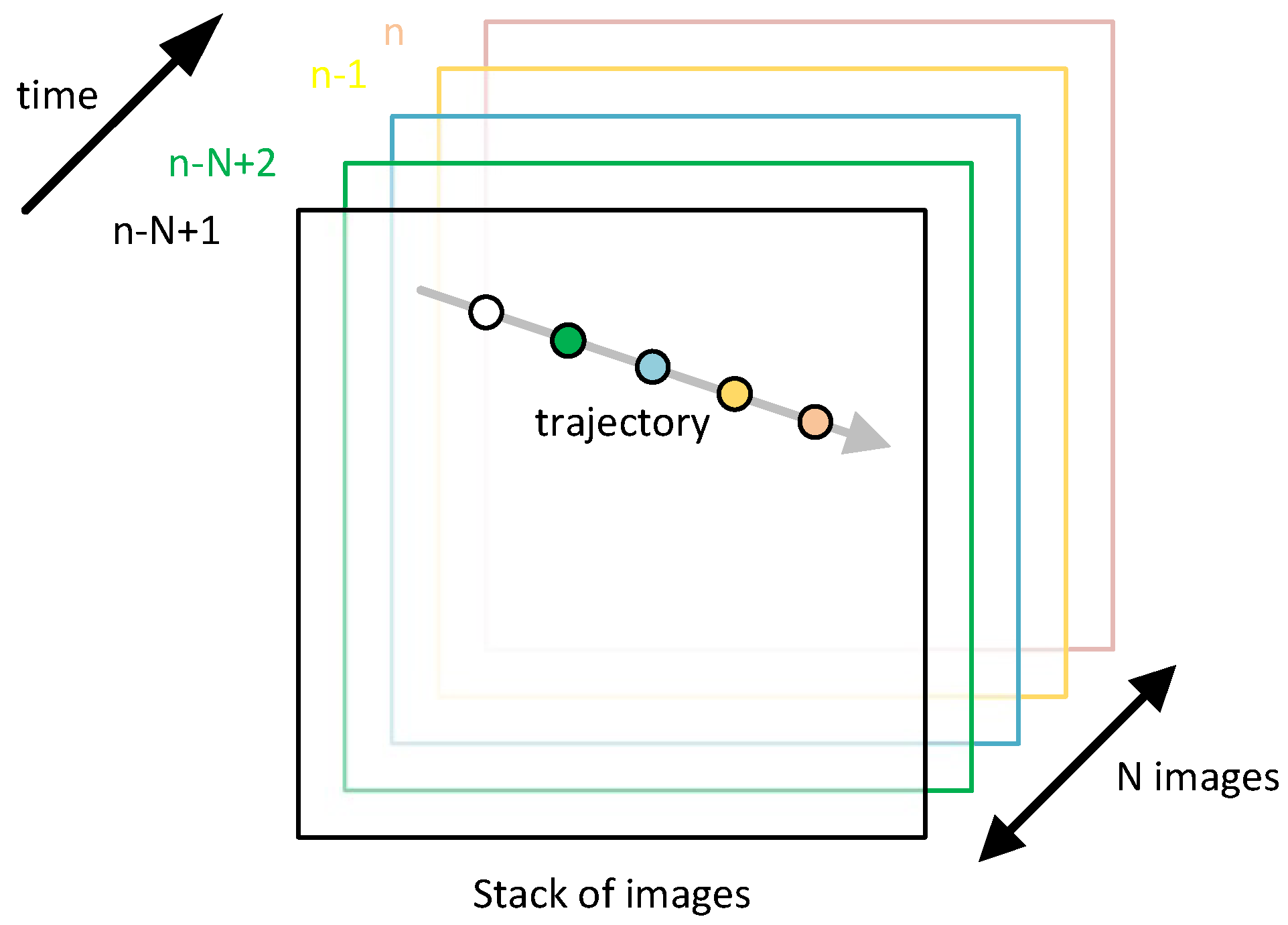
One of the simplest but effective algorithms are 3D filters that perform the accumulation of trajectories for a stack of images. These are non-recursive algorithms, usually using the principle of a sliding window to reduce the number of calculations. The image input stack X has a capacity of N images at time n. The idea of determining the accumulation at time n is shown in Figure 1.

The solution for calculating $n+1$ is to subtract the image $n-N+1$ (oldest) and add the image for $n+1$ (current):

$$Y_{n+1}^v=Y_n^v-X_{n-N+1}^v+X_n^v,$$

(1)

where Y is the output data (image) for a particular trajectory v.

2.2. Optimal Processing and Relationship with ConvNN

Assuming that the input images have the size $M\times M$, determining the number of 3D filters for optimal detection for arbitrarily complex trajectories is possible. Each of the filters accumulate or determines the average value (linear averaging filter) in the stack of images. The location of the object in one pixel with coordinates is $(x,y)$ pair $\left(x,y\in \langle 0,N-1\rangle \right)$. The trajectory of the object in the stack of images is described by a sequence of pairs $(x,y)$:

$$T=\left[{(x,y)}_0,{(x,y)}_1,\cdots ,{(x,y)}_{N-1}\right],$$

(2)

where ${(x,y)}_n$ is the position of the object in image n. There are $M·M$ combinations of object positions on one image frame, and there are ${(M·M)}^N$ combinations of trajectories for the image stack.

The weight values for 3D filters can be calculated (no need to teach) with a simple operation of assigning a value of 1 to the weights of a given trajectory:

$$w_{T{(x,y)}_n}=1,$$

(3)

and the other weights are 0. In the case where $M=100$ and $N=10$, there are $10,{000}^{10}={10}^{13}$ filters and their weight matrix. The optimization of the number of calculations is possible because the matrix of weights is sparse—for each image of the stack, there is only one value equal to 1. Additionally, adjacent trajectories of the same shape could be calculated simultaneously. This leads to the implementation of trajectory calculation through the convolution. The output 2D data (image) then do not correspond to one specific trajectory, but to a whole family of trajectories of identical shape. This allows to reduce the number of calculations by $M·M$ times; however, the number of filters is still very large.

A further reduction in the number of calculations and the number of filters is only possible by considering specific trajectories. In the previous calculations, any combination of the position of the object in the image was assumed. In a realistic case, these are linear trajectories or curves. A characteristic feature is the local proximity of the object location for successive images of the stack.

The implementation of the 3D TBD filter is possible using a convolution such as a convolutional network, but one characteristic of typical ConvNNs, which is the presence of pooling layers [39], cannot be used. Layers of this type allow a gradual reduction of the amount of data between successive layers [40], but they cause a decrease in resolution, and thus, the precision of determining the location of the object.

2.3. 3D TBD Filter for a Reduced Set of Trajectories

The reduction the number of trajectories is possible by specifying more precisely the trajectories that are more realistic for a given class of tracked object. While the introduction of the convolution allowed the optimization due to the translation of the trajectory, it is possible to perform one more optimization with respect to the rotation of the observed space.

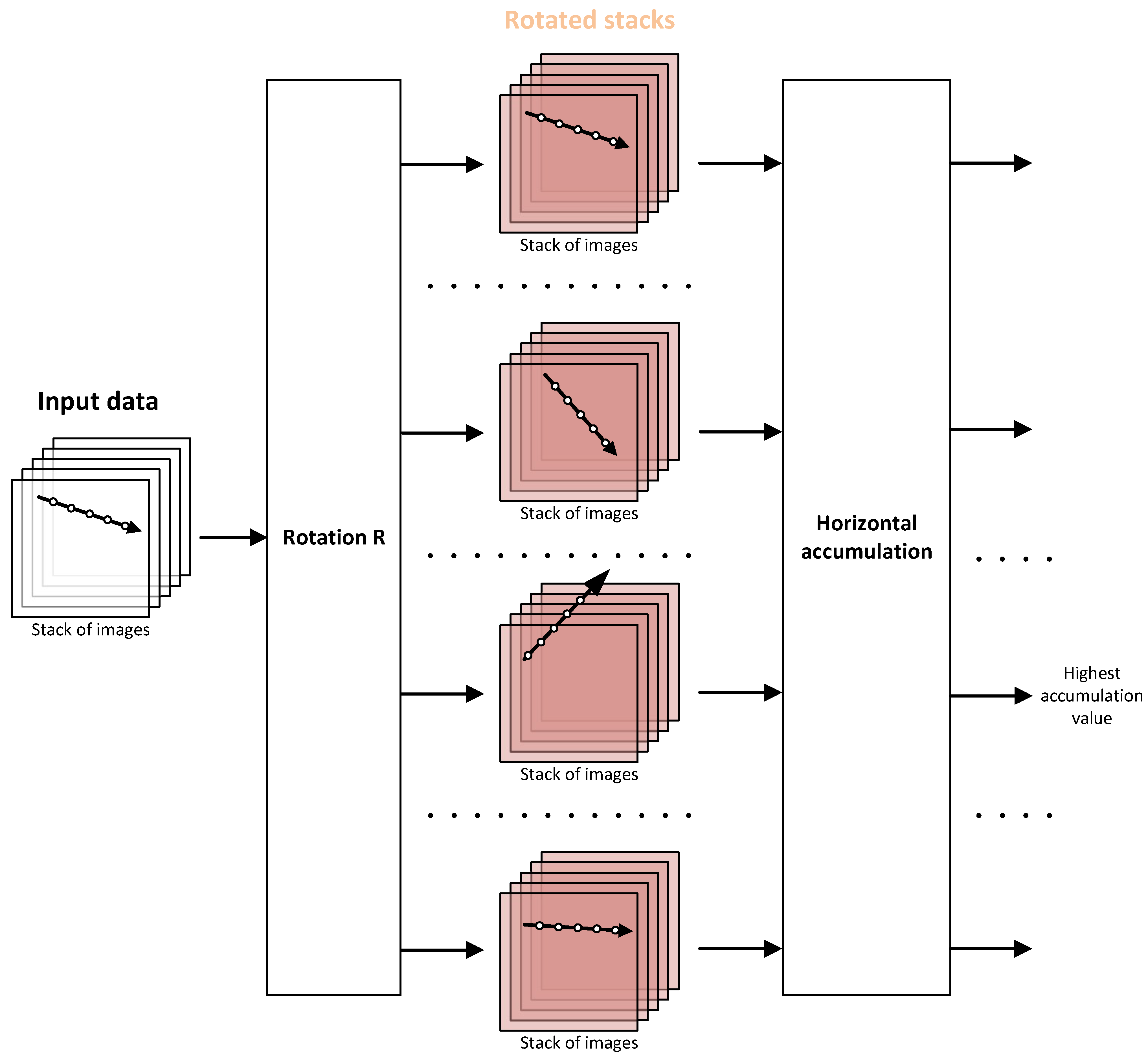
2.3.1. 3D TBD Filter with Rotation Pre-Processing Linear Trajectories

The use of rotation of input images allows to reduce the number of 3D filters. The stack of images is rotated by a specific angle (0–360 degrees or 0–180 degrees) due to symmetry and processed by a smaller set of filters (Figure 2). This does not reduce the computational cost, but only the number of filters, because the same set of filters is used for each rotation angle.

By combining convolution processing and rotation pre-processing, the most common linear trajectories could be detected very efficiently:

$$T=\left[{(x,y)}_0,{(x,y)}_1,\cdots ,{(x,y)}_{N-1}\right]=\left[{(x,y)}_0,{(x,y)}_0+{\overrightarrow{V}}^{2D},\cdots ,{(x,y)}_{N-1}+(N-1){\overrightarrow{V}}^{2D}\right],$$

(4)

where ${\overrightarrow{V}}^{2D}$ is the two-dimensional motion vector of the object between two consecutive observations (images).

Since 3D filters can be oriented in space in one direction, both calculations and memory accesses can be simplified if they are chosen so that only horizontal or vertical trajectories are computed. The trajectories are then given by a simpler formula:

$$T=\left[{(x,y)}_0,{(x,y)}_0+{\overrightarrow{V}}^{1D},\cdots ,{(x,y)}_{N-1}+(N-1){\overrightarrow{V}}^{1D}\right],$$

(5)

where ${\overrightarrow{V}}^{1D}=\left[0,V\right]$ when calculating vertical trajectories or ${\overrightarrow{V}}^{1D}=\left[V,0\right]$ when calculating horizontal trajectories are used. For example, for horizontal trajectories, the formula could be presented even more simply:

$$T=\left[(x_0,y_0),(x_0+V,y_0),\cdots ,(x_0+(N-1)V,y_0)\right],$$

(6)

where V is the velocity of the object in the direction of X (more precisely the modulus of the velocity vector of the object for the two-dimensional case movement).

The computational cost depends on the number of assumed angles and the assumed velocities of the object. The total number of trajectories is $M·M·R·S$, where R is the number of angles and S is the number of one-dimensional velocity vectors V. For example, for $M=100$ and $R=360$ angles and $S=100$ velocity vectors, there are 360M $=3.6\times {10}^8$ trajectories. This is five orders of magnitude less than the initial case.

2.3.2. 3D TBD Filter with Rotation Pre-Processing Linear Trajectories and Two Velocities

With UAVs, speed changes could occur even if the trajectory is linear. Assuming one change in velocity for the stack of images, a modified trajectory model could be proposed and the computational cost determined.

The change of speed is associated not only with the occurrence of two different speeds, but also with the time of the change of speed. Instead of one vector V, there must be two, i.e., $V_1$ and $V_2$. the moment of velocity change is marked as s, where $s\in 〈0,1,2,\cdots ,N-2,N-1〉$. The $V_1$ speed applies until the speed is changed to $V_2$. The number of trajectories is:

$$T=\left[{(x,y)}_0,{(x,y)}_0+{\overrightarrow{V}}_1^{1D},\cdots ,{(x,y)}_s+s·{\overrightarrow{V}}_{2*}^{1D},\cdots ,{(x,y)}_{N-1}+(N-1){\overrightarrow{V}}_{2*}^{1D}\right]$$

(7)

$${\overrightarrow{V}}_{2*}^{1D}={\overrightarrow{V}}_1^{1D}-{\overrightarrow{V}}_2^{1D}$$

(8)

The number of trajectories after taking into account the change in velocity is: $M·M·R·S·S·(N-1)$. The double appearance of S in the computational cost formula is due to two different speeds that can be highly independent, which is typical for many UAVs. The presence of N results from the fact that there are $N-1$ moments of velocity change time.

For example, using the previous assumed values, we have $100\times 100\times 360\times 100\times$$100 \times 10 =360$G $=3.6\times {10}^{10}$ of the trajectories.

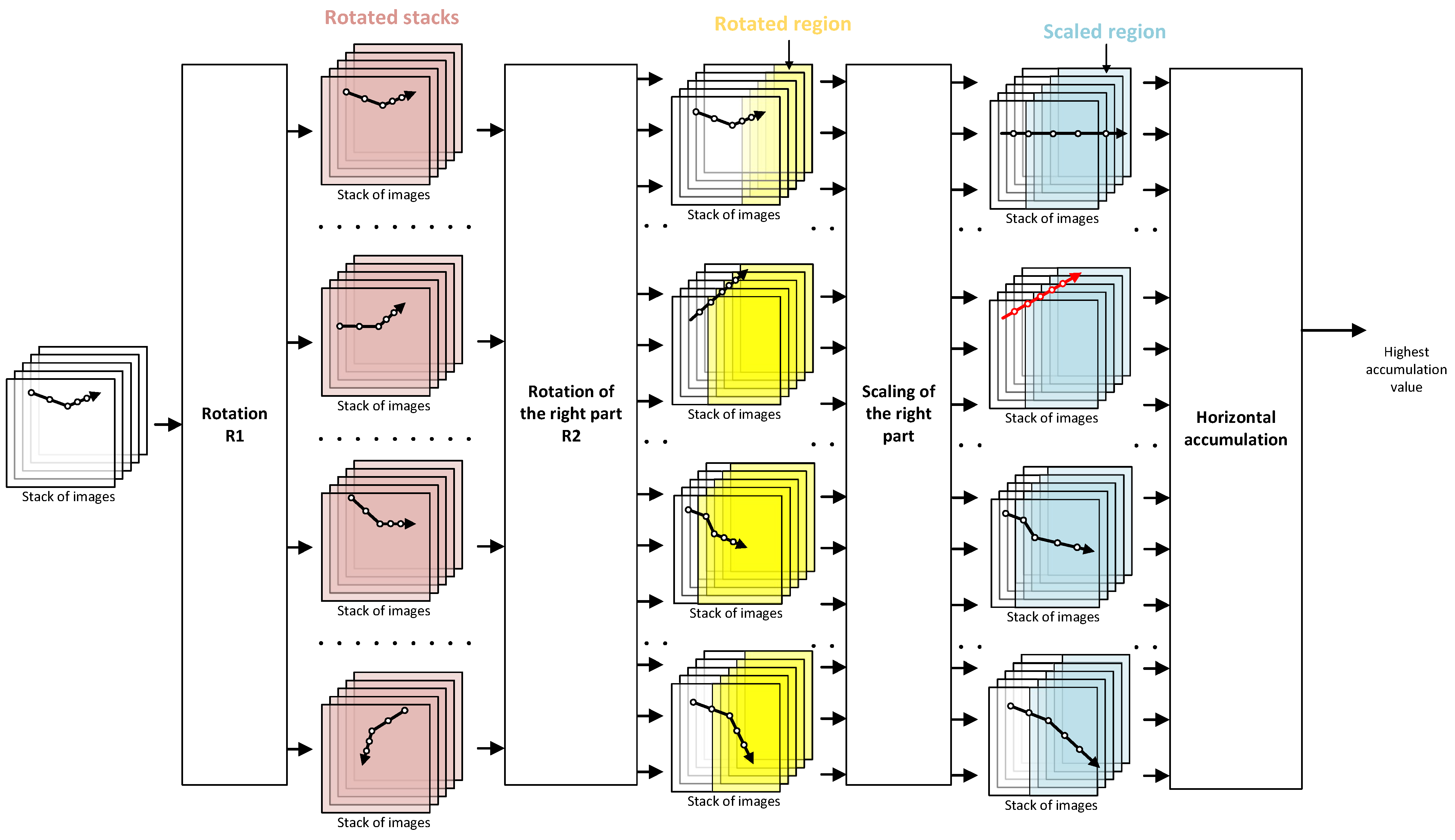
2.3.3. 3D TBD Filter with Rotation Pre-Processing Broken Line Trajectories and Two Velocities

The more general case of a trajectory is when there is a change not only in speed but also in direction (Figure 3). For this purpose, it is necessary to double use the rotation of the input images. Two rotations are not required, becasue the pre-calculated rotated images can be used.

2.4. Kernel Size

There are two strategies for choosing kernels:

• Using the maximum possible kernel, which results from the sum of speed vector modules;
• Optimization of the kernel size due to the location of the velocity vectors.

The first solution is convenient if processing is to take place on a computing unit that has one fixed kernel size defined. In this case, the condition for trajectories normalized to the horizontal direction should be met:

$$\begin{array}{ccc}\hfill W& \ge & (N-1)·v_{max}+1,\hfill \end{array}$$

(9)

$$\begin{array}{ccc}\hfill H& \ge & 1,\hfill \end{array}$$

(10)

where W is the width and H is the height of the kernel. The depth is specified in N because the kernel is three-dimensional.

The kernel should be larger than the results from the formula, which allows learning with the background of the object.

The kernel in the first case is a cuboid (3D tensor) covering all possible locations of the object (Figure 4). The advantage of this solution is that the processing includes not only the local area in the vicinity of the object’s location, but also the background image on the image stack in places where the object has appeared or will appear. The disadvantage is a significantly higher computational cost resulting from the volume of the kernel (the number of pixels of the image stack covered by processing).

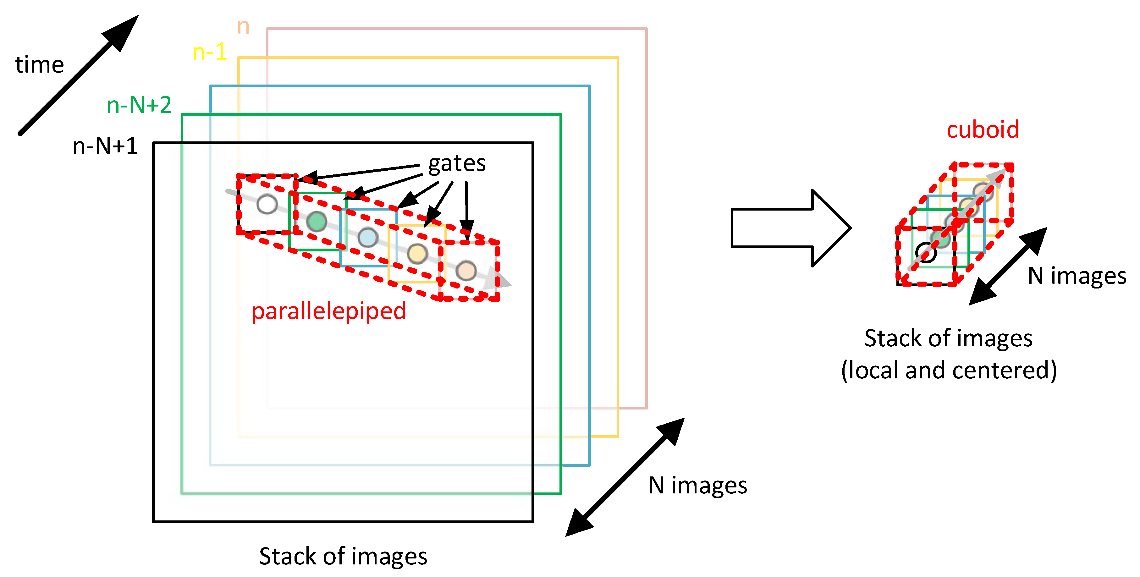
In the second case, it is possible to use tensors in a different shape—parallelepiped (exactly right parallelogrammic prism $C_{2h}$ Order 4). In this case, for each image in the stack, a rectangular area (gate) is used with the center being the estimated location of the object. Due to the movement of the object, the position of the gate is variable, which it creates in 3D parallelepiped space for the image stack (Figure 5). The advantage of this solution is a much lower computational cost, but the consideration of background features is worse than in the first case.

For parallelepiped, the gate size is:

$$\begin{array}{ccc}\hfill W& \ge & 1\hfill \end{array}$$

(11)

$$\begin{array}{ccc}\hfill H& \ge & 1\hfill \end{array}$$

(12)

In the extreme case, only a single pixel ($W=1$, $H=1$) is distributed over all N images of the stack.

The choice of a kernel-shaped solution—cuboid or parallelepiped—is a design decision.

2.5. Image Stack and ConvNN

The previously presented solutions concern the choice of neural network architecture with possible optimization variants in terms of the number of calculations. Since the stack of images can be processed with one neuron, the use of more neurons, also connected in a multi-layer network, gives a more effective system in terms of detection and tracking in the case of various disturbances, for example in the background.

The previous solutions are aimed at rectifying the trajectory and taking into account changes in the speed of the object. This allows a significant simplification of the construction of the neural network in order to reduce the number of neurons and share the results, which is a desirable feature for ConvNN. Since the parallelepiped network gives the highest efficiency in terms of sharing training images, it will be analyzed in more detail in a later section of the article in terms of learning speed.

Since searching all combinations in terms of speed and direction change results in the separation of images from the stack with the image of a specific fragment, a new stack of local images from individual gates can be created from them, which in the case of matching the object’s trajectory is characterized by the fact that the object is in central part of each gate. The local environment is then responsible for the background of the object, or some features of the object if it is not a point object. For example, if it is an airplane, in the central part of the gate there is the center of the fuselage, and in the surroundings there are pixels corresponding to the wings and background.

The task of separating the gate for calculations can be performed by appropriate indexing of image pixels. It is worth noting, however, that since the separation of the gate is nothing more than the imposition of a convolutional filter window, parallel processing of layers (image) can be used analogously, as in ConvNN networks.

3. Results

In the study of the possibility of using ConvNN, the use of the parallelepiped TBD filter was assumed. In the process of testing the effectiveness of ConvNN in the implementation of the TBD task, 10,000 cases were used for various kernel configurations and the signal of the tracked object. In each case, 10,000 cases were trained with 50% of the image stacks with the object and 50% of the image stacks without the object, so that the training set was balanced.

The images were noisy with Gaussian noise with a standard deviation of 10; however, in a later section of the article, the signal and noise levels were scaled so that the standard deviation of the noise was normalized to 1. This is due to the processing of uint8 type image stacks, which additionally causes rounding errors.

Learning for 10 cases of signal values from 0.1 to 4.6 was assumed, where the signal case 0.1 corresponds in the uint8 format to the height of the quantization step before normalization. The total pixel count of the stack was changed from 10 to 1000.

The training process was arbitrarily limited to 3000 epochs with a minibatch size of 10,000. This configuration was selected experimentally so as to obtain a convergence of calculations to a constant accuracy value (even if it was small) for most cases. The accuracy value is responsible for the average probability of correct object detection (true positive) or non-detection (true negative). The learning algorithm was the SGDM (Stochastic gradient descent with momentum) optimizer. The following parameters were used in the learning process:

• Momentum: 0.9;
• InitialLearnRate: 0.01;
• LearnRateSchedule: ‘piecewise’;
• LearnRateDropFactor: 0.1;
• LearnRateDropPeriod: 1000;
• L2 Regularization: $1\times {10}^{-4}$;
• GradientThresholdMethod: ‘l2norm’;
• GradientThreshold: 0.05.

Calculations were made using Matlab R2020a and Deep Learning Toolbox [41] using the following CPU: AMD Ryzen Threadripper 3970X 32-Core Processor.

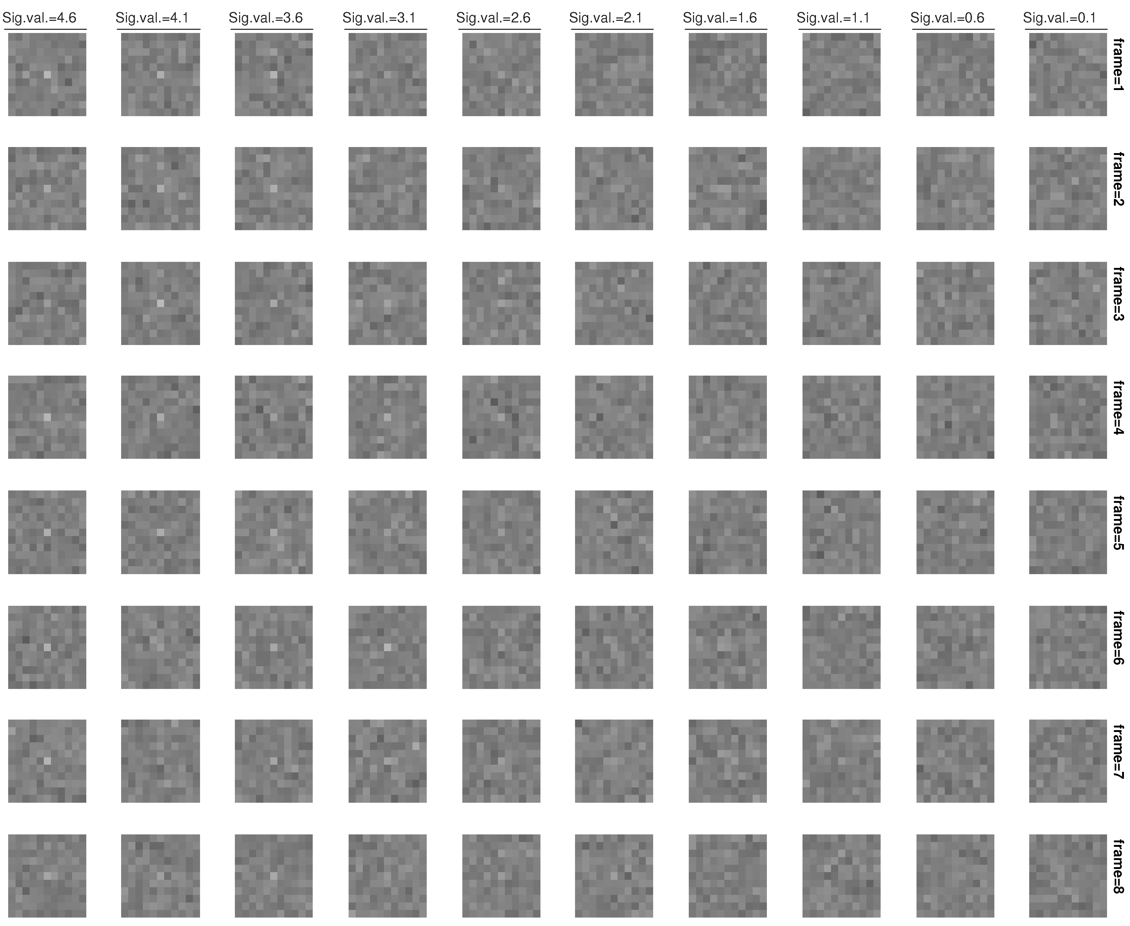
3.1. An Example of an Object Hidden in Noise

To illustrate the scale of the TBD problem, one example case is shown where the stack consists of eight images of size $11\times 11$. The tracked object is located in the central pixel of the images. The kernel structure is shown in the Figure 6, and the configuration in

Table 1. Configuration of kernel from Figure 6.

No.	Name	Type	Activations	Learnables
1	imageinput $[11\times 11\times 8]$ images with ‘zerocenter’ normalization	Image Input	$[11\times 11\times 8]$	-
2	fc 2 fully connected layer	Fully Connected	$[1\times 1\times 2]$	Weights $[2\times 968]$ Bias $[2\times 1]$
3	softmax	Softmax	$[1\times 1\times 2]$	-
4	classoutput crossentropyex	Classification Output	-	-

.

The detection of an object in a single image is very difficult, often impossible (Figure 7) (low signal value level). When the signal level is quite high, it is possible to detect it as a maximum (bright dot) in a single image (in the central position).

Comparing series of images (vertical), it is also possible to detect an object by a human, which results from the fact that the human brain is able to perform data fusion similar to the TBD algorithm. However, this detection is limited to a certain signal-to-noise level.

The ratio of the number of pixels occupied by the object to the number of pixels in the stack is as follows:

$$\frac{P_{object}}{P_{stack}}=\frac{8}{11\times 11\times 8}=0.00826.$$

(13)

where the greater the value of this ratio, the greater the chance of detection, although it always depends on the value of the object’s signal. Different cases for this ratio are shown in Figure 7.

The extreme case is when there is only one image in the stack, and the object takes up only one pixel, which with the same number of pixels gives the result:

$$\frac{P_{object}}{P_{stack}}=\frac{1}{968}=0.001033.$$

(14)

In this case, it is only possible to detect the object, without determining the trajectory.

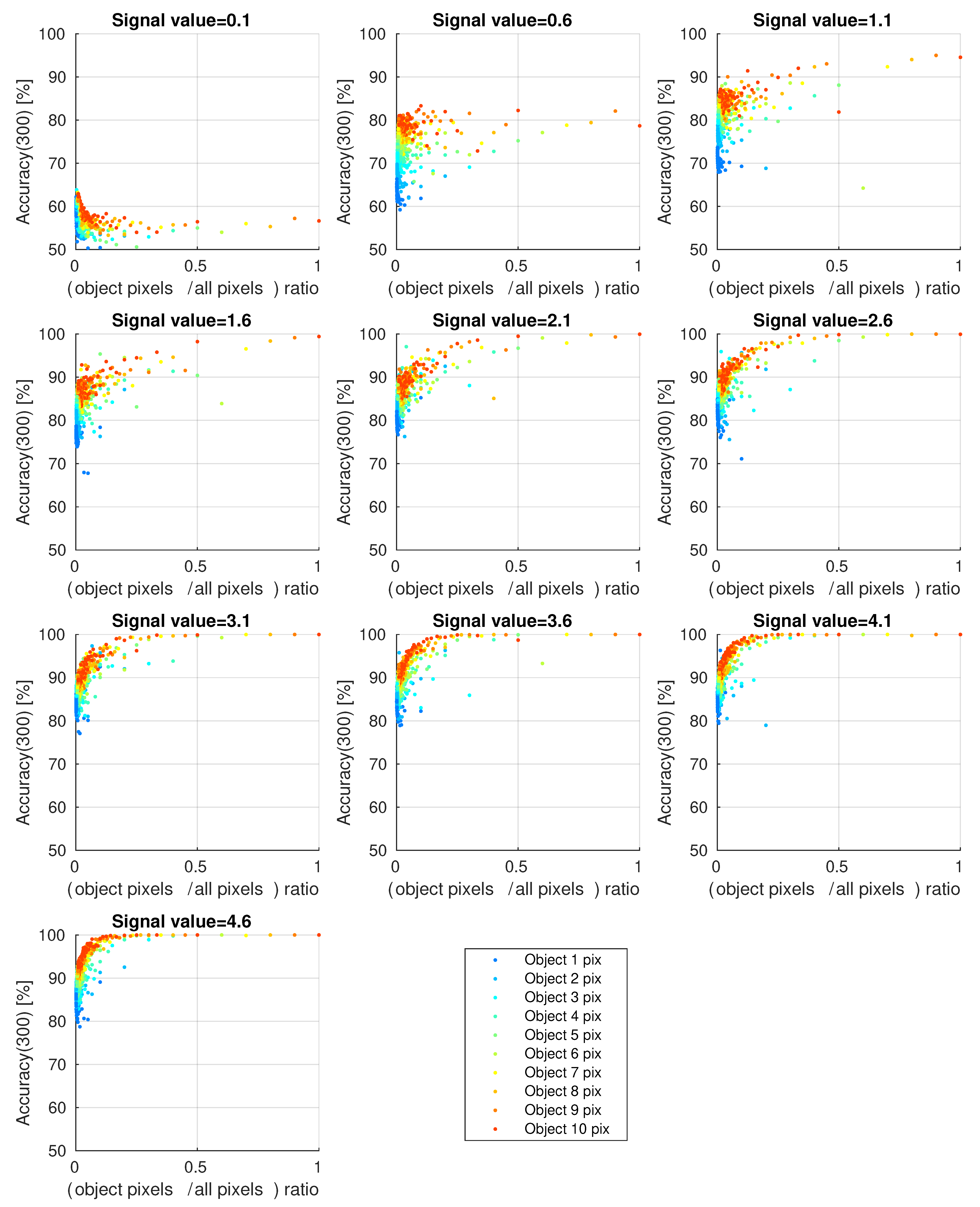
3.2. Accuracy for the Simplest ConvNN-Based TBD

The results of computer simulations for assessing accuracy for various cases are shown in Figure 8 and Figure 9.

The accuracy level of 50% corresponds to an alternative algorithm that gives a random answer. The accuracy level of 100% corresponds to a 100% chance of trajectory detection and estimation.

The results shown in Figure 9 correspond to the state of a stable learning process (after 3000 epochs). Figure 8 shows the impact of premature termination of the learning process (after 300 epochs).

4. Discussion

The detection and tracking of objects hidden in noise is very difficult without the usage of dedicated algorithms (Figure 7). Algorithms using thresholding, both with fixed and adaptive threshold values, are unable to detect most of the objects shown in the figure. Two-dimensional spatial filtering gives some possibilities, but its possibilities are limited because the object takes up one pixel. In the case of larger objects, covering several pixels, it is an interesting solution for computational reasons.

Full use of the information, based on the trajectory, allows the aggregation of the object’s signal values not only from one image frame, but also from the stack. In this case, it is the 3D filtering that is most effective because it uses all available information about the object.

In practice, it becomes necessary to use more advanced methods of aggregating values, because in addition to the object, the background with a characteristics is also recorded. Taking into account the background allows improving the detection quality, but it requires the use of, for example, neural networks to contain knowledge about the background model.

Figure 8 shows the effect of a too short learning process of the simplest ConvNN. Comparing Figure 8 and Figure 9, it is visible that the accuracy value can double and that it can reach 100% if the learning process is long enough. It is not guaranteed that a value of 100% will always be reached, which means that it is necessary to test it (periodically) successively during training.

As expected, the number of pixels of the object affects the accuracy, which was illustrated in such a way that the largest number of pixels of the object is shown in red and the extreme case (one pixel) in dark blue.

In the case of a small number of pixels of the object, detection is possible, even for a single pixel with an accuracy of almost 100%, because the signal is very different from the background. This can be seen in Figure 9 for the dark blue color.

Since the total number of pixels in the stack was changed from 10 to 1000, the ‘object-pixels-to-all-pixels’ ratio is between 0.001 and 1. In the case of a network that is not well trained, this causes a significant decrease in accuracy for small ratio values (Figure 8), while for a well-trained network, the opposite occurs (Figure 9).

Large ratio values apply when the stack is very precisely matched to the size of the object. For example, a value of 1.0 applies to a 10 layer deep stack with a $1\times 1$ pixel window size. This is quite an extreme situation, but it corresponds to a typical 3D velocity filter with a $1\times 1$ window.

This type of solution allows for correct operation with the assumption of noise with zero mean value, and thus, earlier background suppression. This is possible with background estimation algorithms [10], but then the ConvNN capabilities are not used.

In order to perform the TBD task together with background estimation, it is necessary to use the surroundings of the potential object, for example using a $3\times 3$ mask.

In this case, the number of all pixels will be $10\times 3\times 3=90$, which with 10 pixels of the object gives a value of $10/90\approx 0.11$ ratio. This type of analysis allows determine the accuracy for the assumed signal value based on (Figure 9).

An interesting case is when the pixel count of the object is less than the stack depth, regardless of the size of the mask. This situation concerns changes in the signal of the object, which may result from the method of acquiring the signal (image), the use of camouflage or the physical characteristics of the object itself. This example was considered for TBD in [42], where the object can be the rotation of the object (for example satellites). Then, the ratio and accuracy change, which corresponds to the change of colors in Figure 9 towards colder colors.

It is also interesting to compare the results from Figure 9 with sig.val. = 3.1 Figure 7), which is on the verge of human detection. For sig.val. = 3.6 the object is still quite visible, while for 3.1, it is difficult to see. The ratio according to the formula 13 is 0.00826, and the number of pixels of the object is 8. The graph shows that the accuracy is 100%, which means that the TBD algorithm can detect this type of object. For sig.val. = 0.1, the object is very difficult to detect (accuracy 63%), but for 1.1, the accuracy value is about 95%.

5. Conclusions and Further Work

The use of TBD algorithms allows the detection and tracking of objects whose signal could be lost in the background noise. However, each TBD algorithm has its own limitations, which affect the actual detection capability.

The use of ConvNN is possible, which for a $1\times 1$ window comes down to the simplest algorithms of the velocity filter type.

The use of a larger window allows better usage of the image of the object, which could be larger than one pixel, and independently for better detection against the background.

Increasing the window size, however, leads to an increase in computational cost. It is necessary to find a compromise between detection capabilities and computational cost.

The approach presented in the paper allows the estimation of the detection limit for the simplest neural network (single neuron), which allows comparing the results with other more complex networks (including ConvNN), as well as with algorithms that perform image pre-processing to remove the background signal. In such case it is possible to check by comparison whether a more advanced network could works better than the reference solution.

The proposed analysis is especially useful for the parallelepiped model of TBD, because this model processes the least amount of data. Analysis of the trajectory with variable speed of the object and changing direction could be implemented using the solutions presented in Section 2.

It is an open question to construct large neural networks, especially ConvNN, for UAV images that are larger than a single pixel. This topic will be considered in future research.