1. Introduction
Remote sensing requires the construction of real-world dynamic scenarios. Different to optical cameras that capture two-dimensional (2D) images, the laser scanning with Light Detection And Ranging (LiDAR) devices acquire three-dimensional (3D) data for a better representation of spatial geometry. Three-dimensional (3D) structures are described typically in formats of depth image, mesh, point cloud, and voxel, where the point cloud is the most commonly used. However, due to the discontinuous material surfaces or coarse sensor resolutions, the generated point clouds may be locally sparse or missing, which is not conducive to further tasks such as semantic segmentation or classification [
1]. Then, the shape completion is needed to estimate the geometry of objects by reconstructing complete point clouds from partial observations.
Traditional point cloud repair methods are based on the a priori structural characteristics, e.g., symmetry or semantics, to account for the missing points. These methods can only repair point clouds with a low missing ratio and obvious structural features. Presently, deep-neural-network-based methods have been the main stream for point cloud completion. The encoder–decoder framework is the most commonly used completion framework, as has been used in [
2,
3,
4,
5,
6,
7,
8,
9]. Some studies [
10,
11,
12,
13,
14] used the generative adversarial network (GAN) to improve the training of the generator. Recently, the graph convolutional network (GCN) is introduced in some work [
15,
16] to address this topic. Fei et al. [
17] investigated the latest and advanced algorithms for point cloud completion together with their methods and contributions. The related work will be introduced in the next section.
High-quality completion methods emphasize the integrity of details. A 3D shape contains faces, edges, and vertices, which have depth and so they occupy some volume. While all completion methods learn structure from the training set, the downsampled feature extraction modules commonly used in neural networks only capture the main information. This leaves salient points or small irregular surfaces ignored and unable to be reconstructed. Wang et al. [
18] proposed independent learning of edges to capture details. For many objects, such as chairs and computers, edges are sufficient to outline the whole structure. However, an object surface is not always flat, as the shape may resemble the sphere and torus. In this case, subtle shape details cannot be inferred from edges.
In addition to the overall structure, in this paper, we propose to learn contours for point cloud completion. Salient edges and irregular surfaces observed in the training data are expected to be reproduced by the proposed classifier. A new end-to-end neural network is designed for point cloud completion which follows the “point ⇒ voxels ⇒ points” framework in GRNet and VE-PCN, but the encoder and decoder are newly designed with transformers. The classifier is integrated into the decoder with novel loss functions to learn contours.
Although similar edge learning has been used in VE-PCN, our model is compact enough because it requires neither additional branches nor multiple independent downsampling on the input for various grid scales. The contour learning is an improvement toward edge learning for richer a priori knowledge. The self-learning capability of the end-to-end structure makes our model an easier-to-use generator, with the potential to be further combined with more powerful frameworks such as generative adversarial networks and attention mechanisms.
The main contributions of the work are summarized.
- 1.
We propose a new end-to-end network for point cloud completion with newly designed transformers for the encoder and decoder.
- 2.
We propose a solution to learn object contours incorporating critical edges and irregular surfaces for point cloud completion.
The remainder of this article is arranged as following. In
Section 2, related work on point cloud completion is reviewed. In
Section 3, the proposed model structure is presented, and the contour learning is introduced. In
Section 4, an experiment is performed on the ShapeNet dataset to demonstrate the performance of the proposed method by comparing with state-of-the-art completion methods. In
Section 5, the in situ KITTI dataset is used to give a further evaluation of the proposed method. An airbone dataset is tested in
Section 6 for remote sensing evaluation. The potential advantages and disadvantages of the proposed method are discussed in
Section 7.
Section 8 gives the conclusion.
2. Related Work
Deep-neural-network-based methods have been the main stream for point cloud completion to output key points of complete structures and generate denser point offsets based on the key points. The majority of the models are built with convolutional neural networks (CNNs). Achlioptas et al. [
2] introduced the first encoder–decoder framework to implement the deep generation model for point clouds. Yang et al. [
3] improved the auto-encoder model with a graph-based encoder and a two-consecutive-folding-based decoder (FoldingNet) to deform a canonical 2D grid onto a smoother 3D object surface. By combining the advantages of [
2,
3], Yuan et al. [
4] proposed the point completion network (PCN) with fully connected networks to capture the overall shape of point clouds. PCN is further improved in [
5] by folding multiple patches to generate continuous and smooth point cloud surfaces, and then combining these point cloud surfaces. Zhao et al. [
6] suggested the 3D capsule networks as the auto-encoder, where the dynamic routing scheme and 2D latent space were deployed for restoration. To improve FoldingNet, Groueix et al. [
7] proposed AtlasNet with
K multilayer perceptrons to fold out
K surfaces simultaneously. Tchapmi et al. [
8] proposed the topology repesentation network (TopNet) with a multilayer tree structure as the decoder. Xie et al. [
9] proposed the gridding residual network (GRNet) in which a gridding layer and a gridding loss were designed to regularize the disordered point cloud to 3D grids. Junshu et al. [
19] proposed LAKe-Net by localizing aligned keypoints (LAKe) with a topology-aware keypoints-skeleton-shape prediction solution. Yingjie et al. [
20] proposed a novel framework which learns a unified and structured latent space that encodes both partial and complete point clouds. The codec framework shows good performance and excellent efficiency.
The generative adversarial network (GAN) is also adopted for point cloud completion. Zhang et al. [
10] used GAN to reconstruct from a given partial input, which was pretrained on complete shapes to search for latent feature codes. Wen et al. [
11] proposed the cycle transformations between the latent spaces of complete shapes and incomplete ones to build the bidirectional geometry correspondence. Miao et al. [
12] designed a new encoder for neighboring point information in different orientations and scales as well as a decoder to output dense and uniform complete point clouds. Wen et al. [
13] devised a dual-generators framework for point clouds generation, which implemented two GANs to learn effective point embeddings and refine the generated point clouds progressively. Xie et al. [
14] presented the Style-based Point generator with Adversarial Rendering (SparNet) by channel-attentive EdgeConv to fully exploit the local structures. Cheng et al. [
1] proposed a GAN-based dense point cloud completion architecture with skip connections to a fully connected layer-based network for regenerating global feature. The processed point clouds can be successfully used for classification which shows the value of completion. GAN trains the generator in an alternative and adversarial way which is possible for finding better parameters.
The graph convolutional network (GCN) has also been used for the completion of point clouds. Pan [
15] proposed an edge-aware GCN, in which edge features are captured against noise and then propagated with deep hierarchical graph convolution for completion. Shi et al. [
16] proposed a graph-guided deformation network which treats the input data as controlling points and intermediate generation as supporting points, and it models the optimization guided by a GCN. These methods converts vertices into a graph for inference with deep learning.
Although the original shapes are partially missed, the above-mentioned studies output the full region point clouds. To alleviate the error caused by the change of original partial shapes, new methods were proposed to predict only the missing regions. Huang et al. [
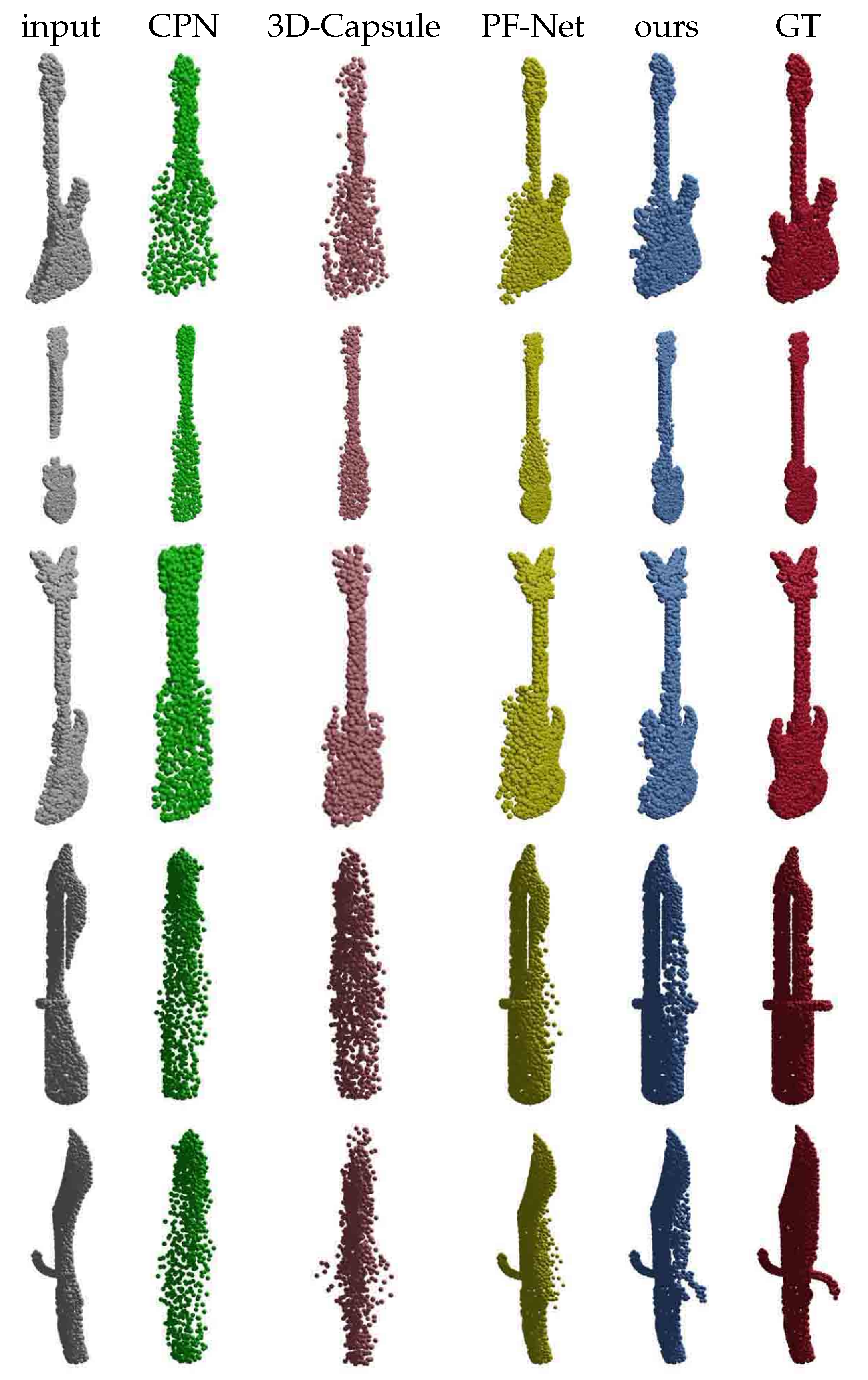
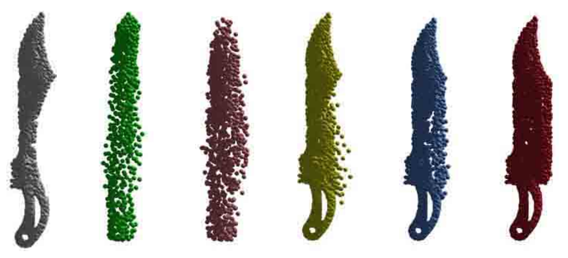
21] proposed the Point Fractal Network (PF-Net) with partial point clouds as the input, and only the missing point clouds are output instead of the whole object. It has a combined multilayer perception to extract multi-scale features and a point pyramid decoder to generate the missing point clouds hierarchically based on feature points. Wen et al. [
22] formulated the prediction as a point cloud deformation process with a novel neural network to simulate an earth mover constraining that the total distance of point moving paths should be shortest.
The key or reference points are the basis to diffuse to more points, but their quality suffers from the adverse sparseness of the point cloud. An area is marked for diffusion when it has one or more points. As a result, the predicted reference points may be unreasonable or inaccurate in case of local sparsity. The homogeneous distribution of the reference points is not assured, which results in the non-uniform density of the diffused point cloud. Instead of predicting key points, GRNet [
9] and VE-PCN [
18] predict the key voxel grids to improve the completion quality. Voxel grids can divide the whole space into regular grids, which ensures that the reference points are not clustered together, thus solving the problem of non-uniform point density after diffusion.
Although the “point ⇒ voxels ⇒ points” framework is successfully used, GRNet and VE-PCN are not ideal enough for completion. VE-PCN is not an end-to-end network due to the independent branches in both the input and the encoder. On the input side, VE-PCN implements multi-scale sampling of point clouds with the help of cascaded farthest point sampling, which results in a high dimensionality of the network input. In fact, multi-scale sampling can be implemented and self-learned in the network, which can reduce unnecessary input. An important contribution of VE-PCN is an edge extraction to guide diffusion, but it depends on a point generator which is not learnable. As for GRNet, the transformation from a point cloud to voxels and the inverse transformation are much too simple, which relies only on the eight convolutional layers for grids completion. GRNet also ignored the varying point importance as generated by the edge branch in VE-PCN.
3. Methodology
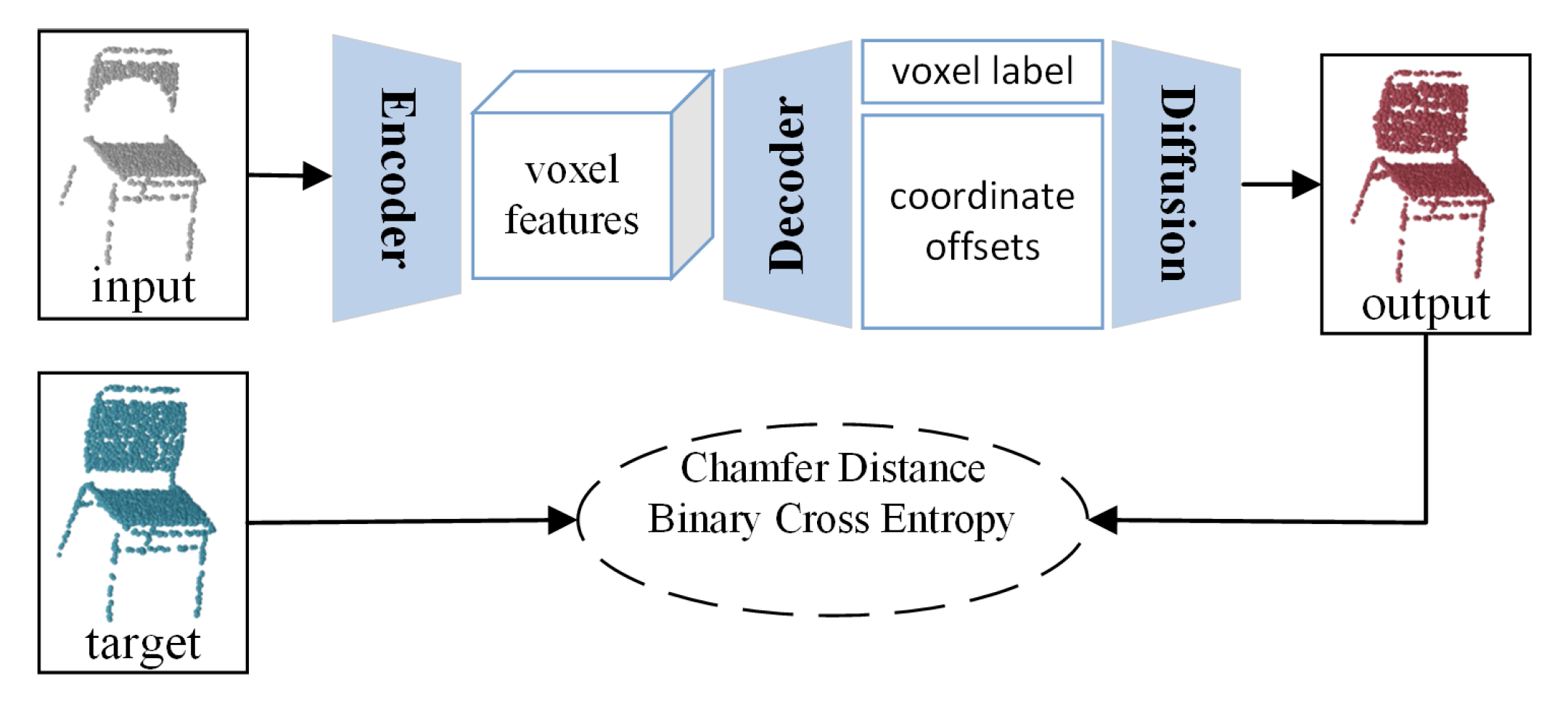
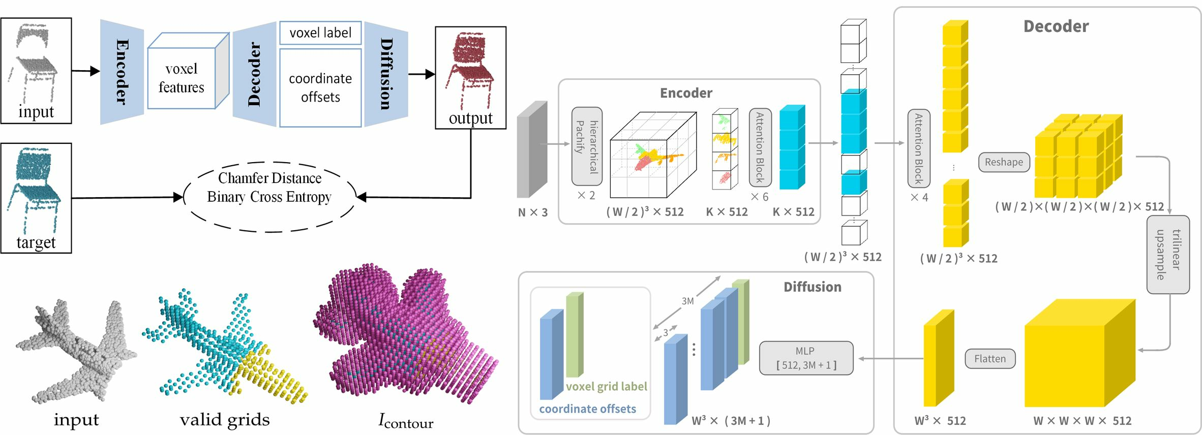
This section will detail the newly proposed model. The overall framework is composed of an encoder, a decoder, and a diffusion module (
Figure 1). The codec framework is a general solution to point cloud processing. However, the new idea is that our encoder produces voxel features to indirectly extract point cloud features, which is guided by a classifier for diffusion. The proposed model is named as Point-Voxel-Point Network and abbreviated as PVP-Net for short.
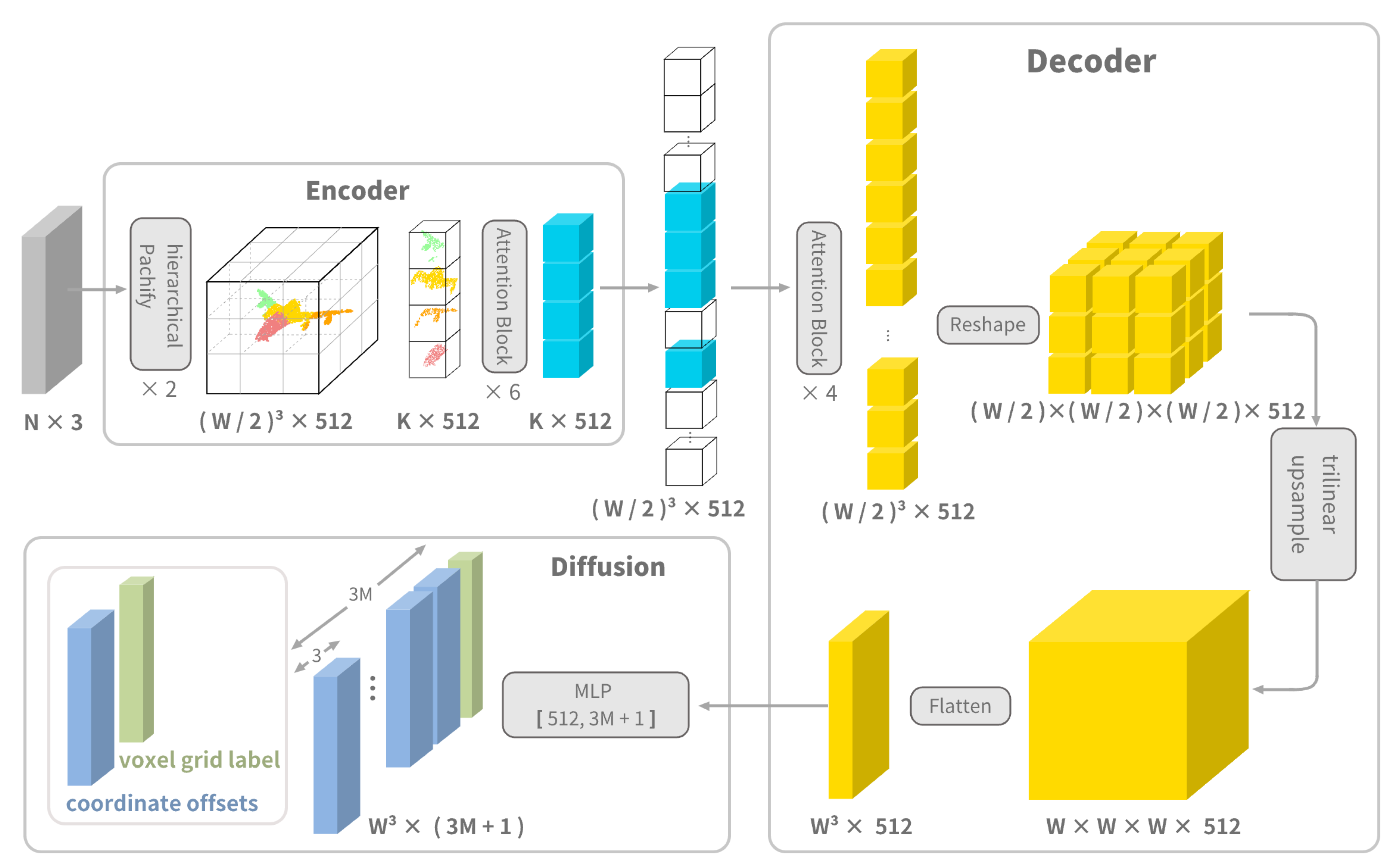
3.1. Encoder
The structure of the encoder is shown in the upper part of
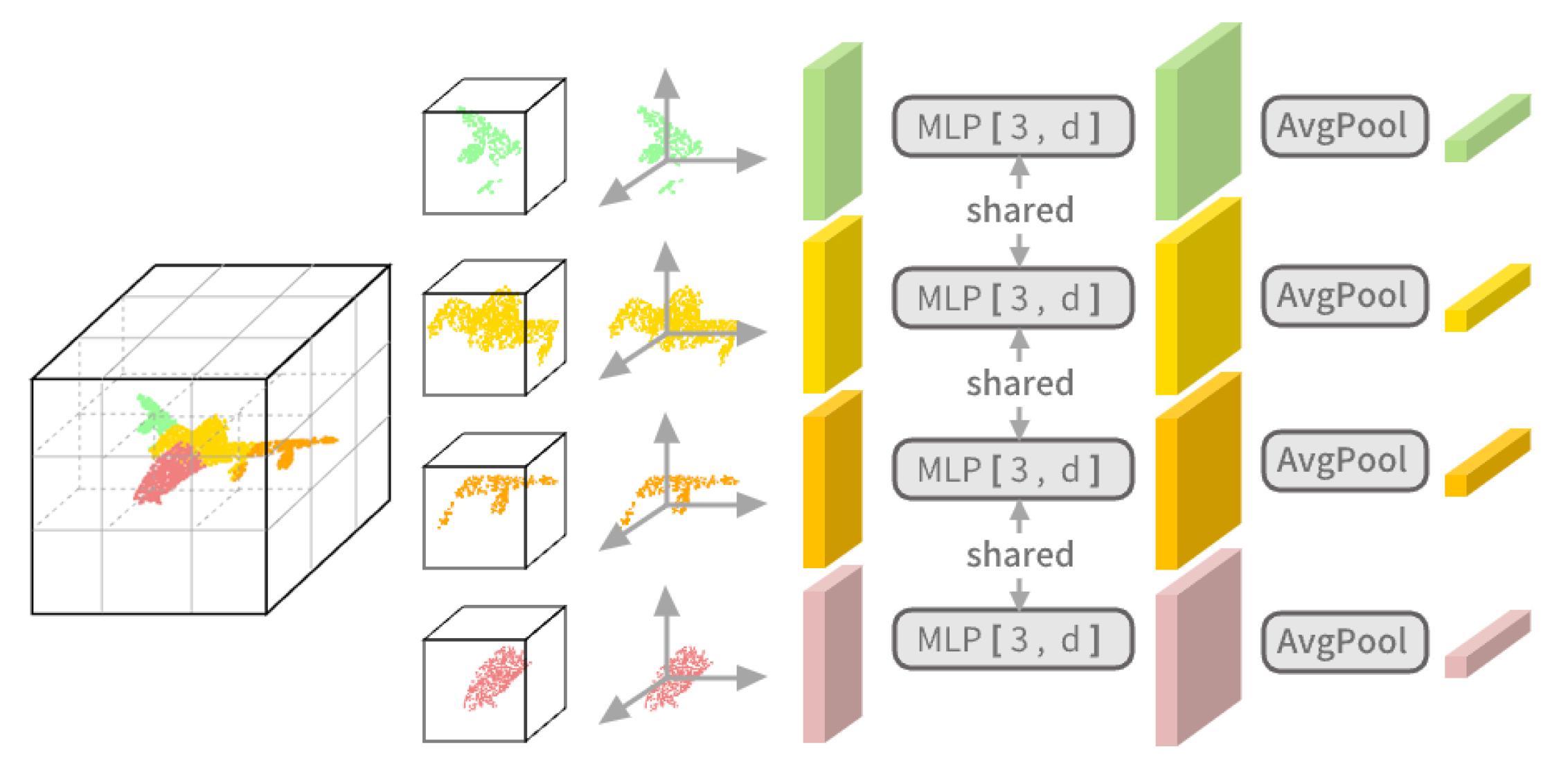
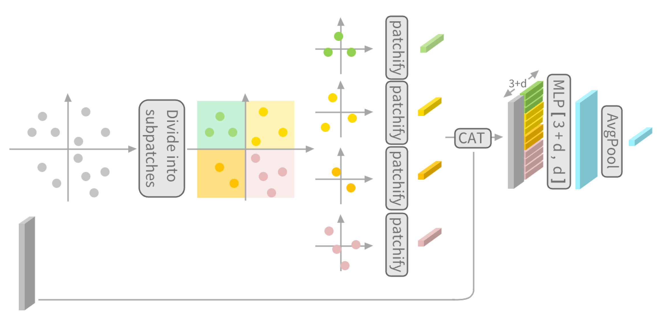
Figure 2. The point cloud coordinates are normalized to [−1, 1] and input to the encoder. The encoder consists of a Patchify module and an Attention module. In the Patchify module, the point cloud is divided into non-overlapping grids, and their features are encoded separately. In our method, the feature of a grid is recorded as a vector of length 512. The Patchify operation consists of four steps. First, the space containing the complete point cloud is uniformly divided into
grids. Second, the points within a grid are transformed to a local coordinate system with the grid center as the origin. Third, each local point coordinate is mapped to a feature by a multilayer preceptron (MLP). Lastly, all the features in a grid are aggregated into a vector by an aggregation function (e.g., AvgPool or MaxPool) to represent the patch feature. For an empty grid (without points in it), its patch feature is a learnable vector. This vector is shared by all empty grids and is determined during the optimization process. The Patchify process is shown in
Figure 3.
Instead of the standard Patchify operation, a hierarchical Patchify strategy is suggested. The size of W in Patchify has a significant impact on the network. The decoder spans the space to grids. Since the transformer is used in the decoder, the interaction in transformer requires the square number of grids (). The feature of a grid is coded in 512 words (2048 bytes). On the one hand, if the value of W is large, optimization may not be possible as the transformer is memory intensive. For example, is a typical value which requires over 2048 gigabytes video card memory for GPU acceleration. On the other hand, a small W value may lose the scale details of the point cloud too quickly, resulting in the loss of geometric information. To solve this problem, a multi-stage strategy is proposed to gradually reduce the scale while keeping as much geometric information as possible.
As shown in
Figure 4, the core of the hierarchical Patchify is grid subdivision and feature merging. It divides the grids into smaller grids for Patchify and then merges the features. In our method, a 2-stage hierarchical Patchify is used. For the 2-stage hierarchical Patchify process, the point cloud is pictured as a
grid that is initially divided into coarse grids with the number
. Each coarse grid is further divided into eight fine grids, which undergo the Patchify to give a
matrix where
n is the point number in a coarse grid and
d is the feature length. In other words, each point is given a vector description of length
d, and all the points in a fine grid share the same descriptor. The
matrix is concatenated with the original coordinate matrix
to fuse the feature of the coarse grids recorded as a
matrix.
The features extracted by hierarchical Patchify are fed to the attention module. Taking the strategy of masked autoencoders (MAE) [
23], only features of non-empty grids are extracted. They are combined with position codes and then go through a series of transformer blocks for encoding. Since the encoder works only on non-empty grids, the amount of operations and speed of the operations are greatly reduced.
Specifically, let
F consist of non-empty voxel features.
, where K is the number of non-empty voxels and
.
F is input to the attention blocks after summing with the position encodings. The 1D position embedding is used, which consists of
of sinusoidal positional encoding computed according to [
24]. There are two sub-layers in each attention block: a multi-headed attention layer enabling interaction between the input features, and a forward network. The multi-headed attention layer
is defined as
where ⊕ denotes the concatenation along the channel direction.
,
,
, and
are learnable projection matrices. Each attention head employs a single-head dot product attention
The parameters of the attention block are set to
and
.
Q,
K, and
V are all set to
F; that is,
F is mapped to
after each self-attention block. The forward network operates on each feature in the network separately. Following the implementation in [
24], a two-layer feed-forward network is used with a rectified linear unit (ReLU) activation function after the first layer.
3.2. Decoder
The structure of the decoder is shown in the lower part of
Figure 2. The input to the decoder is the features of all patches, including the empty patches of the empty grid and the non-empty patches of the encoder output. The decoded result is obtained by adding positional encoding to all the patch features and then passing through a series of attention blocks with the same configuration as the encoder and a trilinear upsampling layer.
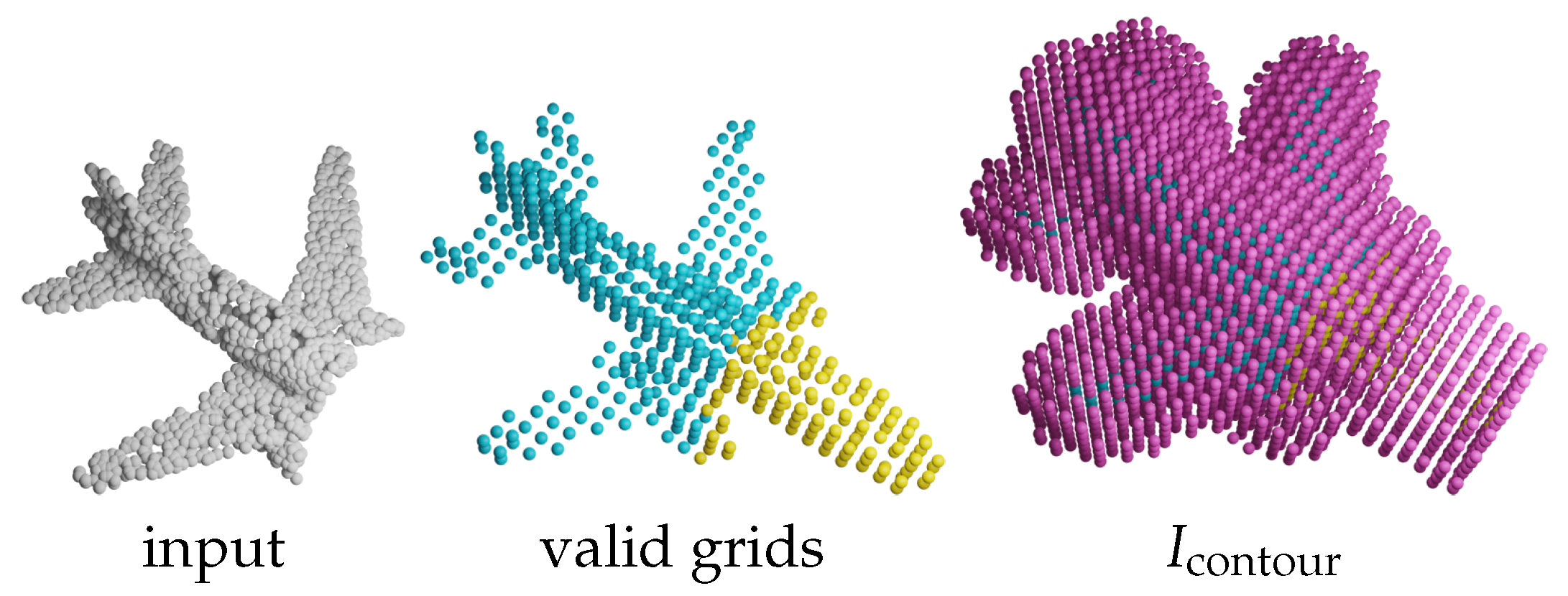
3.3. Diffusion
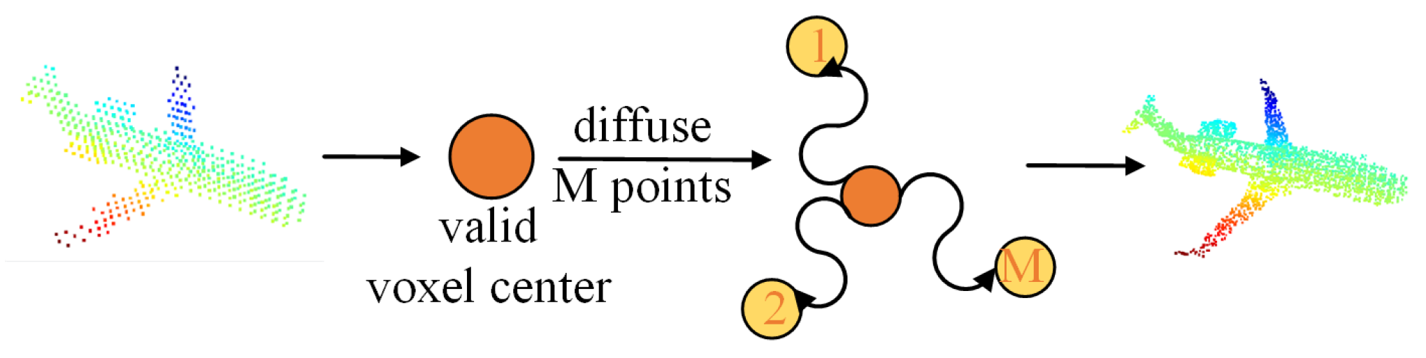
The output of the decoder consists of two parts—a grid label and some coordinate offsets of the diffused points relative to the center of the voxel grid to which it belongs. The number of diffused points is preset as
M that is linked to the density of predicted points. A typical value for
M is 5 for the ShapeNet dataset [
25]. Once again, it is noted that the reference points of our method are defined as the regular grid centers instead of the known or predicted points in a point cloud. The diffusion operation is illustrated in
Figure 5. For each valid grid, diffusion is performed within the grid with
M point coordinates calculated using the offsets from the network output plus the coordinate of the grid center.
The grid labels generated by the decoder judge the validity of a grid. The label values are floating points which are mapped to the range [0, 1] through the sigmoid function. When the sigmoid value is greater than 0.5, the grid is valid and qualified for diffusion. In other words, invalid grids are not diffused because they may correspond to a vacant or extremely sparse space. Obviously, most grids are marked as invalid due to the sparsity of point clouds.
As far as the prediction regions are concerned, our method can perform completion both globally and locally. Completion is global when diffusion is performed within all valid voxels and no input points are kept. For local completion, all the input points are remained, and diffusion is performed within all valid voxels to ensure that the point number in each valid voxel is no less than M. Both methods have advantages and disadvantages. Local completion is preferred because our method is distinguished in judging the validation of voxels.
3.4. Training and Loss Functions
Complete data are required in training. The majority of the point coordinates are randomly extracted from a complete point cloud data and fed into the proposed network for prediction. There will be position deviation between the predicted point cloud and the true point cloud. In this case, the cyclic Chamfer distance is commonly used to evaluate the error between the point cloud coordinates obtained by diffusion and the ground truth, which is defined as
and calculated with
Here,
and
represent point clouds;
and
are the point numbers in these two sets;
x and
y are the coordinates of the point in each cloud;
represents the minimum distance between a point and a point cloud. Equation (
4) searches for the average minimal distance in both directions.
The effectiveness of each grid is also concerned in our method but is not measured yet. To evaluate the impact of invalid grids, the binary cross-entropy is appended as an additional loss, which is defined as
and calculated with
where
N is the number of all labels,
represents the label for the
grid, and
represents the probability that
is valid.
is denoted as 1 or 0 to indicate that the
grid is valid or not, respectively.
is obtained using the sigmoid function on the first output of the last fully connected layer.
We observe that the importance of grids varies and can be classified into four categories, as shown in
Figure 6.
denotes the valid grids that exist in both input and target.
denotes the valid grids missing in the input but present in the target. Analogous to the edges in VE-PCN,
denotes the invalid grids that are adjacent to valid grids to construct a contour covering the surface of an object. The adjacent grids are the neighbored 26 grids in the
space except for the center grid.
denotes the invalid grids other than
. Clearly, it is easy to identify
and
but difficult for
and
as they are the focus of completion. Therefore, the weights for these grids are different. The general classification error is defined as the confidence loss
and calculated with
The overall loss is the sum of the above two loss functions
6. Experiment on the ALS Dataset
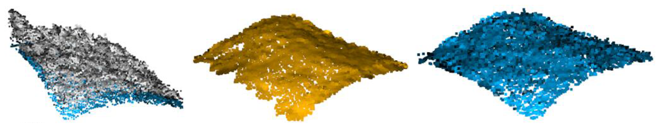
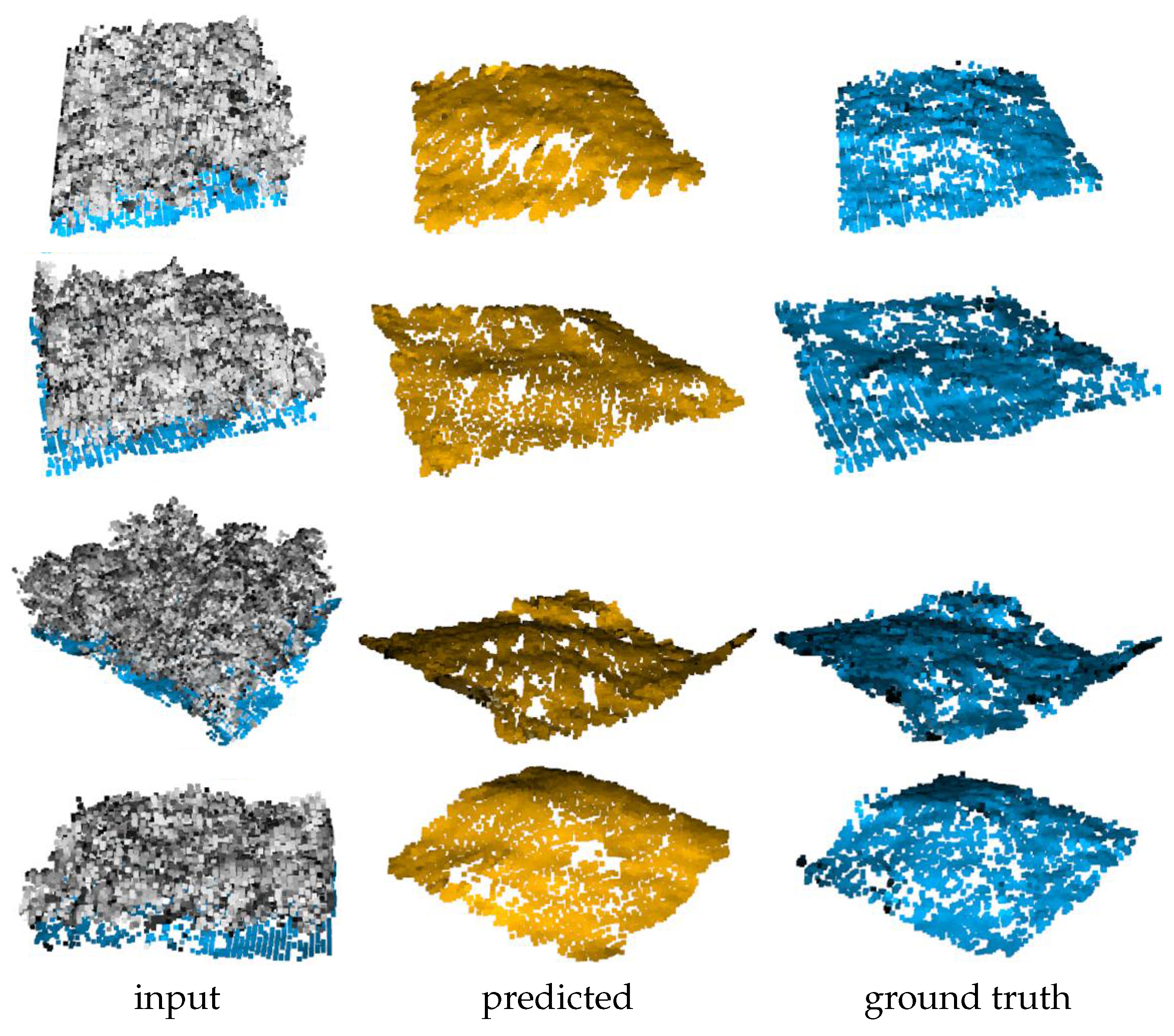
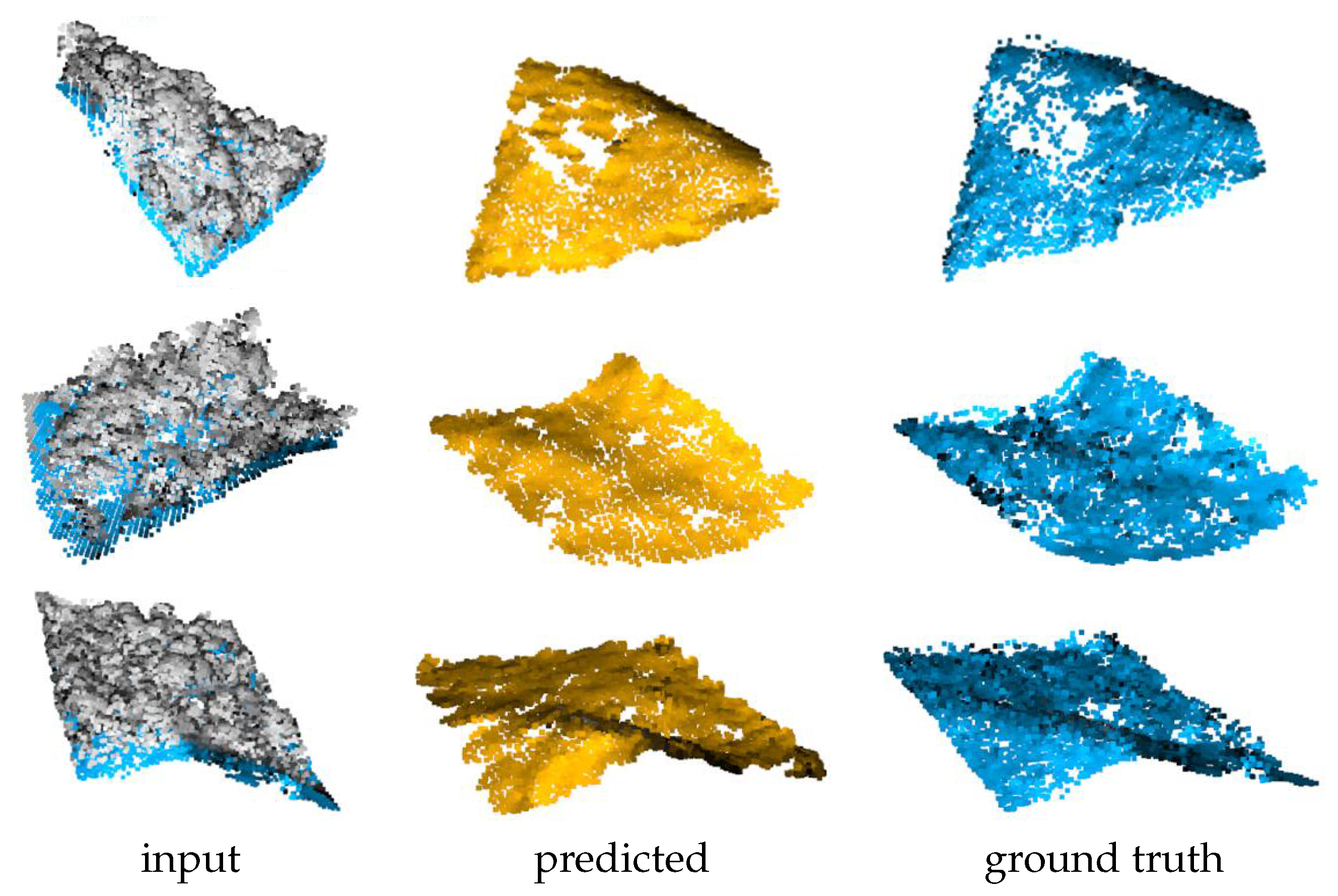
Ground completion is a key task. The 3D scenes obtained by matching satellite images usually do not contain ground structures, which is not applicable to some applications monitoring land cover changes, such as the height estimation of crops or forests. If the ground structure can be predicted using a point cloud completion model, canopy height can be obtained from the difference between vegetation and ground. This can lead to finer biomass assessment. To this end, an experiment is performed for remote sensing purposes.
The airborne laser scanning (ALS) dataset is used in the experiment, which contains three point cloud scenarios: dense vegetation plus gentle slope, dense vegetation plus steep slope, and sparse vegetation plus steep slope. The point clouds in the dataset are labeled with ground points and non-ground points. As for the scale of training and test, the first scene contains 794 training samples and 88 test samples, the second scene contains 1625 training samples and 180 test samples, and the last scene contains 294 training samples and 32 test samples, respectively. The total training samples are 2713 and the total test samples are 300. In the training stage, ground points were removed from the scenes as the input, whereas the output of the model presented the missing ground structure. In the sparse + steep test, each point cloud sample contains roughly 12,000 points, of which the number of ground points is about 3000, with a missing percentage of about 25%. In the dense + slow and dense + steep tests, each point cloud sample contains roughly 18,000 points, of which the number of ground points is about 4000, for a missing proportion of about 22%.
Our method is compared with PCN, PF-Net, VE-PCN, PS-Net, and LAKe-Net. The parameters for the proposed method were the same as those used in the ShapeNet test, except that the network was trained 200 epoches for the ALS dataset. The experimental results are shown in
Figure 13,
Figure 14 and
Figure 15. The evaluation in
Table 3 shows clearly that our method can achieve the best completion results compared with competing methods.
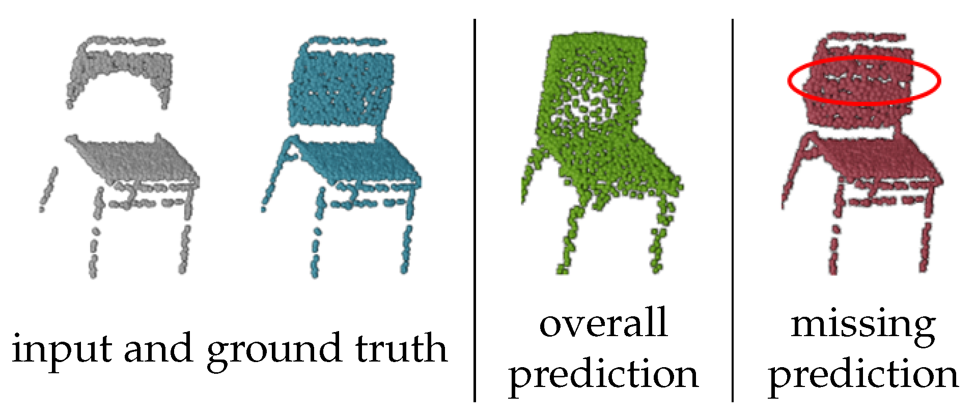
7. Discussion
Attention and contour learning are newly designed in our model. The necessity of the two models is uncovered in this section. In addition, the point cloud completion methods can be divided into two categories, namely overall prediction and missing prediction. Both types have advantages and disadvantages. Both methods can be used for the proposed method, but the missing prediction is preferred in the experiment. The detail loss and structural integrity are observed to compare the difference of the two methods.
7.1. Ablation Study
An ablation study was conducted to verify the effectiveness of the model structure and the newly proposed loss function. In the study, the attention blocks in the encoder and decoder are replaced with the U-Net structure based on 3DCNN. The effect of using and not using contour loss is compared. The modified model was trained and tested on ShapeNet. The experimental results are shown in
Table 4 and assessed with the Chamfer distance. The results show that the best results can be achieved by using both attention blocks and contour loss, which indicates that both the model and the loss function are effective and critical for performance improvement.
7.2. Impact of Contour Learning
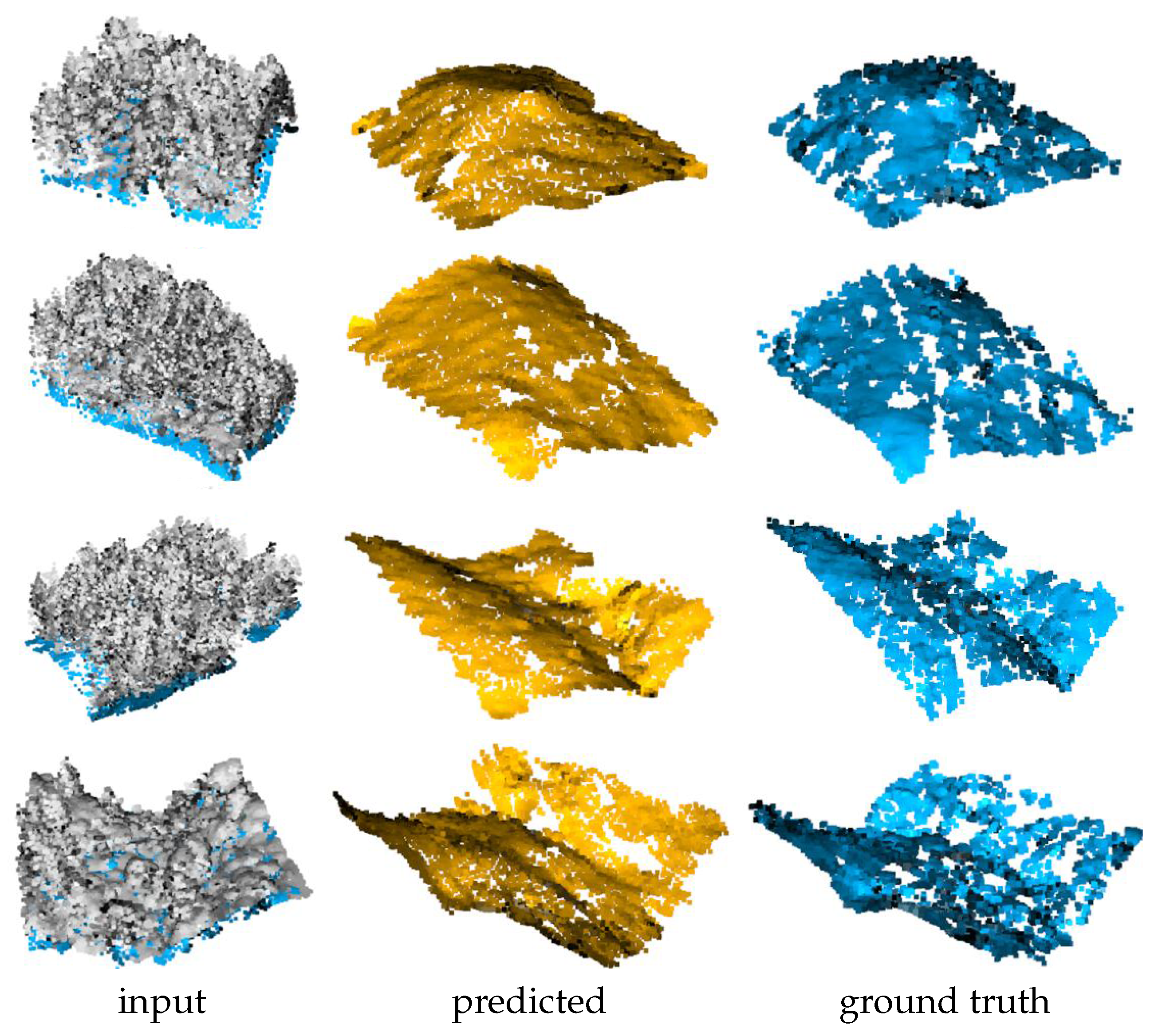
In the newly proposed cost function, the importance of the grid is assigned to be variable. Its necessity can be presented by a confidence map. In order to plot the heatmap under the top view as shown in
Figure 16, the middle layer of the voxel grid label predicted by the network is taken out. The results show that when the contour loss is not used in training (by setting
), the classification results of the contours are of low confidence. When the contour loss is used, the confidence of the classification is significantly improved, and a clearer contour can be seen from the confidence map.
7.3. Impact of Grid Size
The grid size is given by the important parameter W for tradeoff. A larger value of W allows for a higher voxel resolution, thereby preserving more shape details. However, it also increases the computational burden. On the other hand, an extraordinary large value of W implies capturing detailed contours, which brings challenges on the complexity of the network and the amount of training data. From the perspective of numerical evaluation, there exists an optimal W that matches the density of the points. In other words, a larger value of W is not necessarily better nor is a smaller value. The optimal W is linked to the point density.
In the experiment, W was set to 26 for all the tests. This value is the maximum value that can be supported by the computational resource used in this study (NVIDIA 2060 with 6GB memory). The training spends around 3 days for the ShapeNet dataset and 1 day for the KITTI dataset and the ALS dataset. Since the point cloud data have been normalized to the range of [−1, 1] before being inputted to the network, the grid size is 2/26.
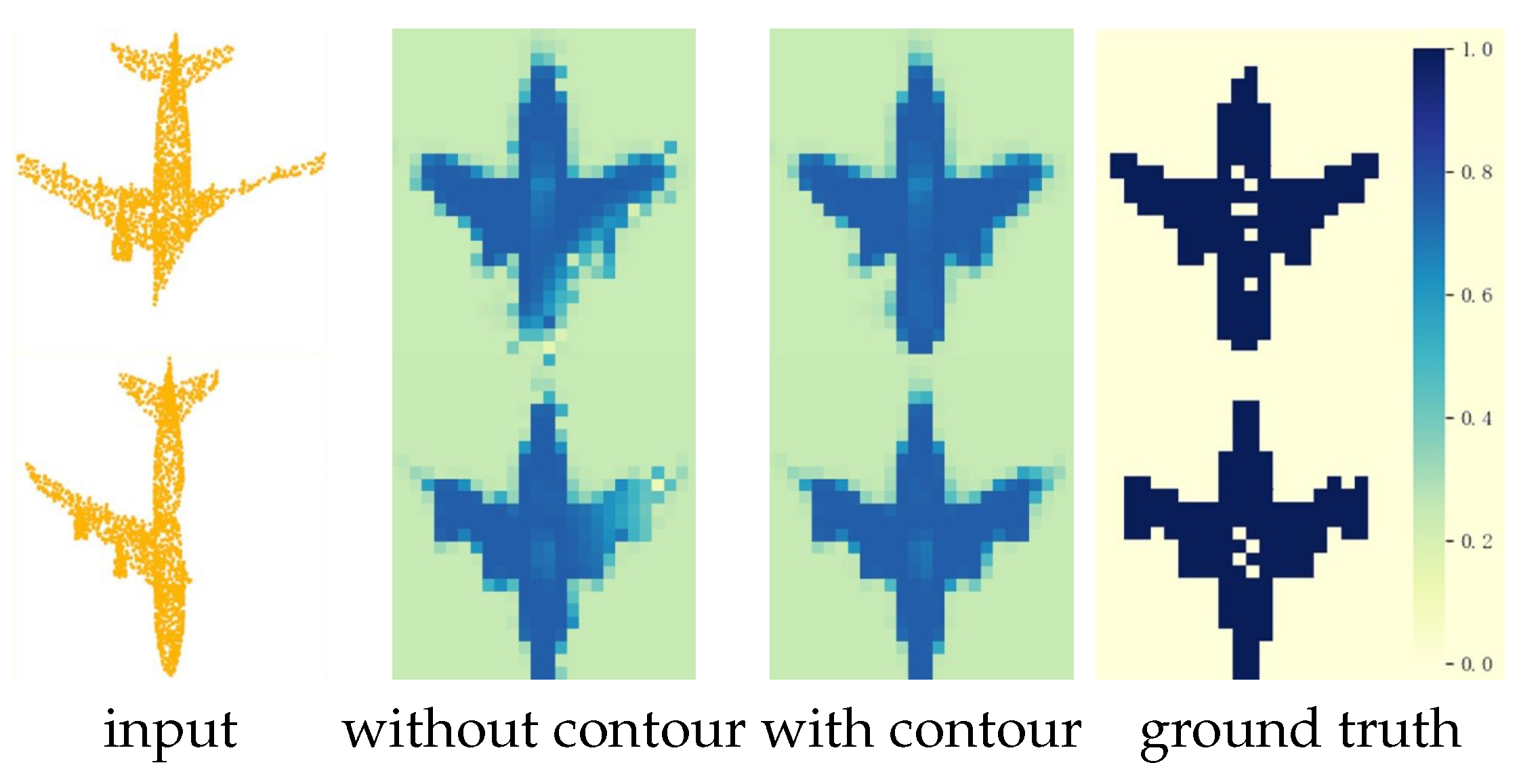
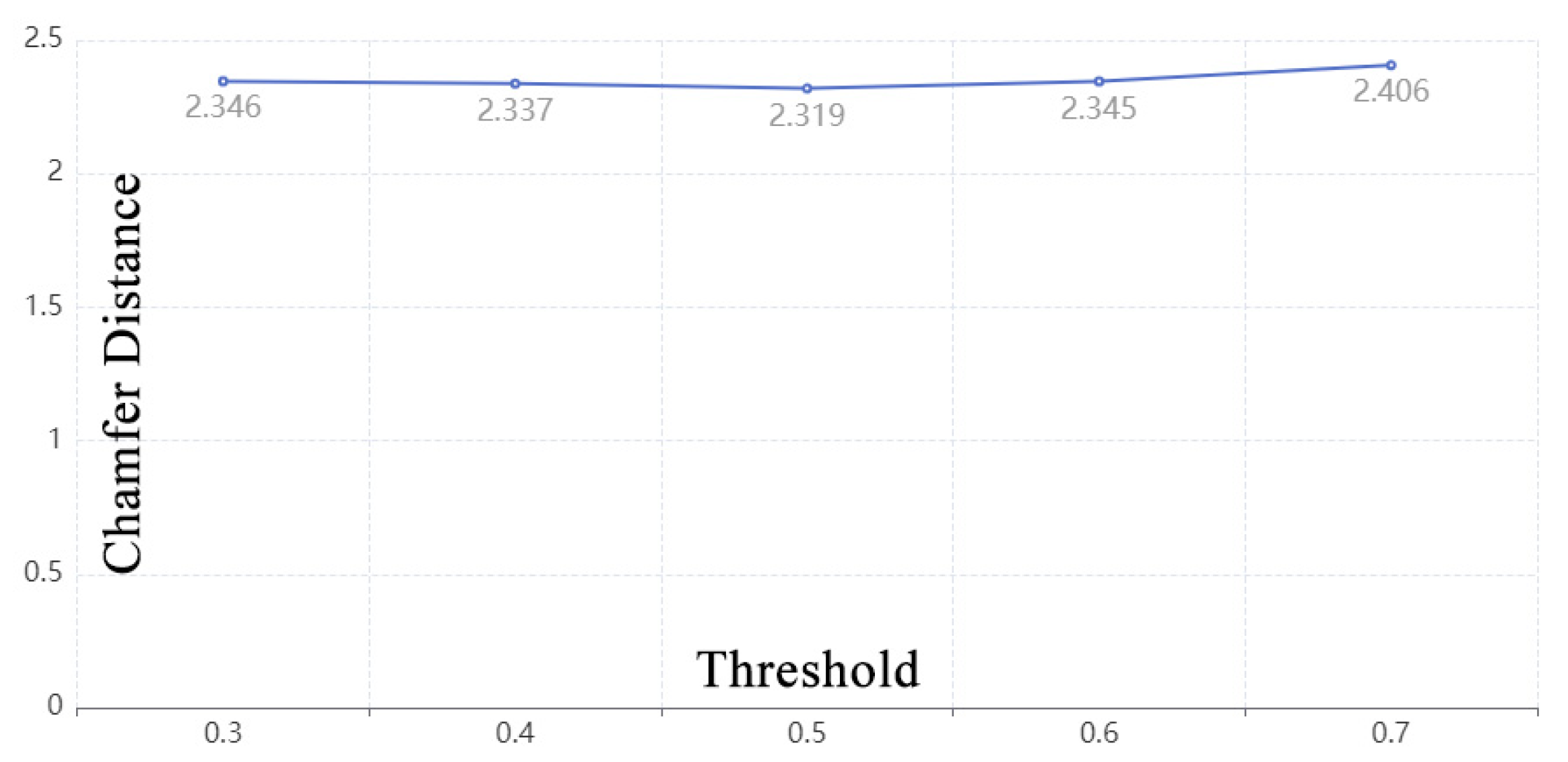
7.4. Impact of Decision Threshold for Contour Learning
When the sigmoid function is used for normalization, the decision threshold for a typical binary classifier is commonly set to 0.5. However, Esposito et al. [
30] found that 0.5 is suboptimal for imbalanced data. Point cloud completion also faces the challenge of data imbalance, so 0.5 may not be the ideal threshold. To find the truth, an experiment was added by changing the threshold within the range of [0.3, 0.7] and comparing the results on ShapeNet, as shown in
Figure 17. The results indicate that setting the threshold to 0.5 is appropriate. The difference between the worst and best results is only 0.087.
7.5. Detail Loss
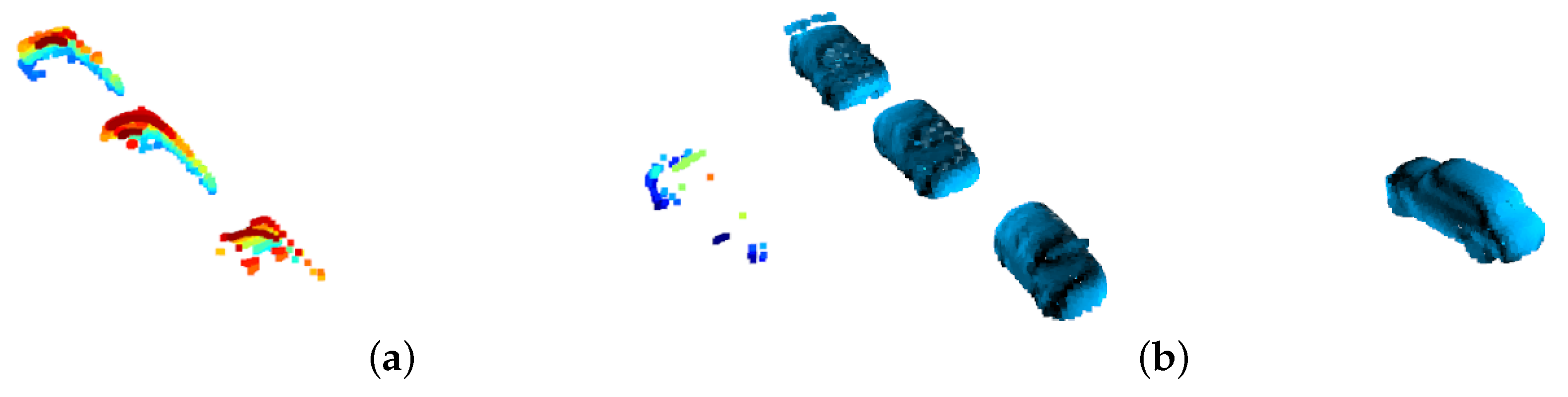
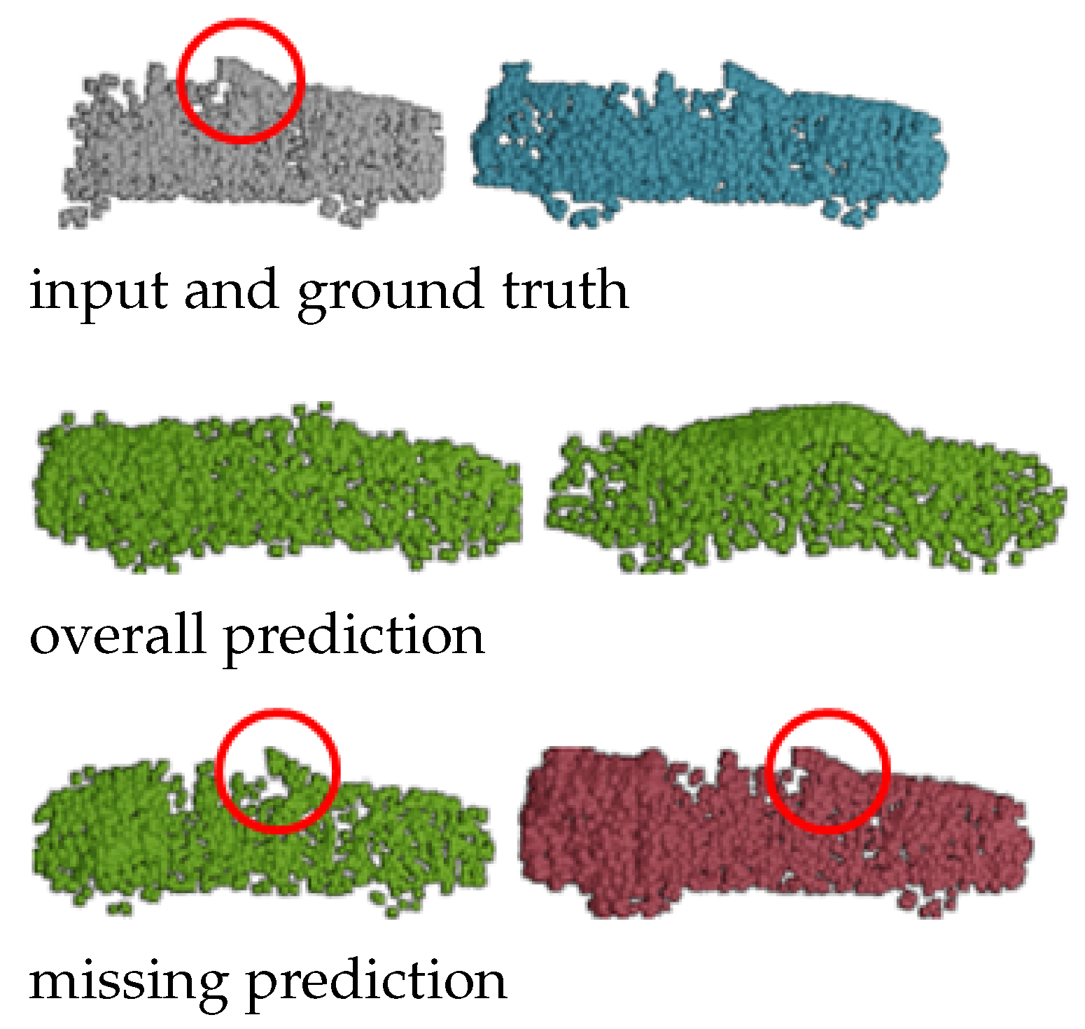
In terms of details in the prediction results, the missing prediction methods tend to produce more details than the overall prediction methods. Missing prediction transfers the full details of the input clouds to the output part. Overall prediction, however, takes no additional constraint on the input, which is easy to lose details when the network reconstruction quality is not satisfied enough. Taking the car completion results in
Figure 18 as an example, the completion results of the overall prediction methods fail to reconstruct the detail of the front windshield, while the completion methods of missing prediction can retain it.
7.6. Structural Integrity
From the perspective of surface smoothness, the overall prediction results have smoother surfaces, while the missing prediction results may have gaps between the input and output.
Figure 19 presents an example for integrity check. Despite the loss of detail or uneven density in the overall prediction, the final result is visually complete.
8. Conclusions
A learning-based model is proposed for precise and high-fidelity point cloud completion. In the method, the regular voxel points are selected as reference points to ensure uniform point density, and an end-to-end neural network is constructed for the cyclic conversion framework between a point cloud and voxels. A classifier is trained to remove the vacant or sparse grids and keep the valid voxels for diffusion. The deliberately designed loss function makes the classifier learn the prior knowledge of object contours.
The proposed method is named Point-Voxel-Point Network, or PVP-Net, tested on the ShapeNet dataset, and compared with 11 state-of-the-art algorithms. The Chamfer distance evaluation confirms that the new method outweighs all competing methods by 14% or higher. The visual comparison shows that our method can produce uniformly distributed points with higher details. Additional experiments on the KITTI dataset and the airbone laser dataset confirm the effectiveness of the proposed method for the in situ completion.


