1. Introduction
Global Navigation Satellite Systems (GNSS) positioning is fundamentally based on the principle of three-dimensional (3D) trilateration, whereby spatial distances (called pseudo-ranges in GNSS terminology) from the GNSS satellite in Earth’s orbit to the GNSS receiver are determined based on the indirectly derived signal propagation time. GNSS signals are electromagnetic waves, i.e., radio waves in the L-band (1–2 GHz) of the electromagnetic spectrum, that propagate at the speed of light [
1]. In such radiofrequency systems, antennas are key elements because, by transforming electromagnetic waves into voltage, they essentially represent an interface between the incoming GNSS signals and the GNSS receiver. For more fundamental information regarding GNSS transmitter and receiver antennas, their design, and performance aspects, interested readers are referred to [
2,
3]. Today, many GNSS applications require millimeter accuracy, but for such requirements to be fulfilled, all influential factors down to the centimeter and millimeter level need to be understood and accounted for. The receiver antenna phase center correction (PCC) model is an essential influencer in high-precision GNSS positioning applications based on carrier phase measurements.
In an idealized situation, the electrical phase center (PC) of a receiver antenna can be defined as a geometrical point to which all registered phase measurements refer [
4]. As the antenna PC is, generally, within the antenna, it is unreachable, and its connection to a physical point or “conventional” terrestrial measurements is needed. However, due to the antenna’s physical and electromagnetic properties [
2], its PC is changing and varies depending on the incoming GNSS signal’s direction, frequency, and intensity and, as such, deviates from an ideal omnidirectional radiation pattern [
5,
6,
7,
8,
9]. Fundamentally, every incoming signal has its own electrical PC. Such changes in the location of the antenna PC cause advances and delays in carrier phase measurements and, thus, elevation-, azimuth-, and frequency-dependent range errors. Therefore, to solve these range discrepancies, antenna calibration is needed.
Generally, antenna calibration is a procedure of determining the relationship between the antenna’s mean phase center (MPC) and an easily accessible physical feature point, i.e., the antenna reference point (ARP), as well as determining the range corrections as a function of satellite position (azimuth and elevation angles) and signal frequency. Today, GNSS antenna calibration methods can be divided into
relative field calibration,
chamber calibration, and
absolute field calibration [
9,
10,
11,
12]. In Rothacher et al. [
13], Seeber et al. [
14], and Mader [
15], the relative field calibration method is introduced and described. Within this method, the antenna to be calibrated, i.e., the antenna under test (AUT), is placed at the calibration field together with a reference antenna (REF) in a short baseline setup. Carrier phase observations are collected at both stations simultaneously from all satellites in view and, in the subsequent data processing stage, the PCC model of the calibrated antenna is determined relative to the reference antenna, i.e., only the difference in PCCs between the reference and calibrated antennas can be determined. Thereby, the reference antenna’s PCC model can conventionally be taken as zero or a precisely known value if the antenna itself has been previously independently absolutely calibrated. The main drawback of the relative calibration method is that the calibration results suffer from multipath [
10,
16]. The chamber calibration method is a laboratory method where the antenna to be calibrated is set up in an anechoic chamber together with a signal source. The transmitter generates an artificial GNSS signal and, to sample the entire antenna hemisphere, the antenna is rotated, or the transmitter is moved [
17]. It is worth noting that chamber calibrations enable the determination of the antenna PCC model in an absolute sense, i.e., independently on any reference antenna, but are extremely infrastructurally and process-wise demanding [
10]. To overcome the drawbacks of relative calibrations, in 1997, Wübbena et al. [
5] presented the basic concepts of a calibration method that is based on the rotation of the antenna to be calibrated at the field around at least two axes. Further improvement and automatization by using a calibrated robot, originally published by Wübbena et al. in 2000 [
6], led to the development of the absolute field calibration method, which is, today, the
de facto standard for GNSS antenna calibrations. Within this method, similar to the relative calibration, the AUT is placed at the calibration field together with a REF antenna in a short baseline setup, but a device is used to precisely rotate and tilt the AUT with respect to the current satellite constellation. During calibration, real satellite signals are tracked, and raw carrier phase observations are collected simultaneously on both stations. Further data processing enables the elimination of the reference antenna PCC, which ultimately leads to an absolute PCC model for the AUT.
Antenna calibration models can also be divided into individual and type-mean models. An individual antenna calibration model is the result of one or several individual calibrations of one specific receiver antenna in combination with or without a radome. Such a model applies only to that individual antenna (of that specific serial number) with the radome that was installed during calibration. On the other hand, the type-mean antenna calibration model is the result of multiple calibrations of several antennas of the same type (different serial numbers) in combination with or without a radome. Such individual calibration results are averaged, and the final type-mean model refers to that antenna type and radome.
The first automated absolute field calibration system was developed in 2000 by Geo++ GmbH in collaboration with the Institute of Geodesy of the University of Hannover, Germany [
6,
18]. Recently, Geo++ GmbH upgraded its system for absolute multi-frequency and multi-GNSS calibrations [
19]. In parallel to the operational calibration system, the Institute of Geodesy of the University of Hannover is developing its new experimental system [
7,
9,
20,
21]. In addition to the above-mentioned two, the Geo++ GmbH calibration system is additionally operational at Geoscience Australia in Canberra, Australia [
22], and Senatsverwaltung für Stadtentwicklung Berlin (SenB), Germany [
19]. Furthermore, in addition to all of the above, there are five absolute calibration systems operational or under development worldwide: the National Geodetic Survey in the USA [
23,
24], GNSS Research Center of the Wuhan University in China [
8,
25], the Institute of Geodesy and Photogrammetry at ETH Zürich in Switzerland [
10,
11,
16], Topcon Positioning System in Italy [
26], and the Institute of Geodesy and Civil Engineering of the University of Warmia and Mazury in Poland [
12]. According to the available literature, the Institute for Geodesy and Geoinformation of the University of Bonn in Germany is the only institution that has developed and operates antenna chamber calibration [
17,
27]. Furthermore, it is worth stating that, currently, only Geo++ GmbH, the Institute of Geodesy of the University of Hannover, SenB, and the Institute for Geodesy and Geoinformation of the University of Bonn, all in Germany, are approved by the International GNSS Service (IGS) to provide absolute antenna calibration results [
28].
Antenna calibrations are exchanged in the ANTEX (The ANTenna EXchange) format (
.atx file extension), defined and maintained by the IGS Antenna Working Group [
29]. In November 2006, in parallel with the adoption of the ITRF2005, the IGS implemented a major transition from relative to absolute antenna calibration models (IGSMAIL-5438) [
30]. Recently, with the start of GPS Week 2238 (as of November 27th, 2022), the IGS adopted the new IGS20 reference frame, which is closely related to the ITRF2020, and together with that transition, an updated set of satellite and receiver antenna calibrations, including the IGS20.atx (IGSMAIL-8238 and IGSMAIL-8256) [
31,
32]. The current official IGS ANTEX file, containing type-mean multi-frequency multi-GNSS calibrations for all antenna types operated in the IGS network, can be downloaded from the official IGS website [
33].
From the recent literature, it is evident that receiver antenna calibration is still an important topic in many GNSS applications. Several studies have shown that the omission of, or use of inadequate, antenna calibration models leads to significant result discrepancies [
34,
35,
36,
37]. Furthermore, with the development and modernization of GNSS [
38] and the availability of new GNSS signals, the need for their calibration emerges. Today, the lack of consistent multi-frequency multi-GNSS antenna calibration values is a challenging issue [
9,
21]. Several research results show significant antenna calibration pattern differences between different institutions and calibration methods [
39,
40,
41,
42]. Accurate and consistent antenna calibration models are, among others, essential in the realization of global terrestrial reference frames [
43,
44,
45].
Consequently, at the Laboratory for Measurements and Measuring Technique (LMMT) of the Faculty of Geodesy at the University of Zagreb in Croatia, the development of a new antenna calibration system has begun from scratch. The developed system is an absolute field calibration system that utilizes a Mitsubishi industrial robot. The main objectives of this research, after comprehensive initial tests, are to examine the repeatability of individual calibrations of the same antenna and to validate the LMMT calibration results with independent calibrations obtained by an IGS-approved institution. This paper presents initial antenna calibration results for the Global Positioning System (GPS) L1 frequency (ANTEX consistent frequency code G01).
The remainder of this paper is organized as follows.
Section 2 elaborates on the following: the theoretical background of the generally adopted standard receiver antenna PCC model, the new calibration method and underlying PCC estimation model used, and, lastly, a detailed description of the receiver antenna calibration system developed at LMMT.
Section 3 presents, analyzes, and discusses the gained experimental research results. Finally,
Section 4 evaluates the research objectives and concludes the paper.
2. Materials and Methods
2.1. The PCC Model
A simplified generic GNSS observation equation for carrier phase measurements
from receiver A to satellite
i, for any frequency, in units of length (meter) reads [
12,
16,
46]:
where
is the geometric distance,
the speed of light,
and
the receiver and satellite clock errors,
is the relativistic effects term,
is the combined satellite and receiver antenna PCC value,
is the receiver hardware delay,
is the satellite hardware delay,
is the tropospheric signal delay,
is the ionospheric signal delay,
is the wavelength of the GNSS signal,
is the integer phase ambiguity in units of cycle,
is the carrier phase wind-up (PWU) effect in units of cycle,
is the phase multipath term, and, lastly,
is the residual error term, which mainly refers to phase observation noise. It is noted that the satellite antenna PCCs fall outside the scope of this research and, therefore, are omitted in further mathematical formulations.
According to the IGS convention and the ANTEX definition of antenna corrections [
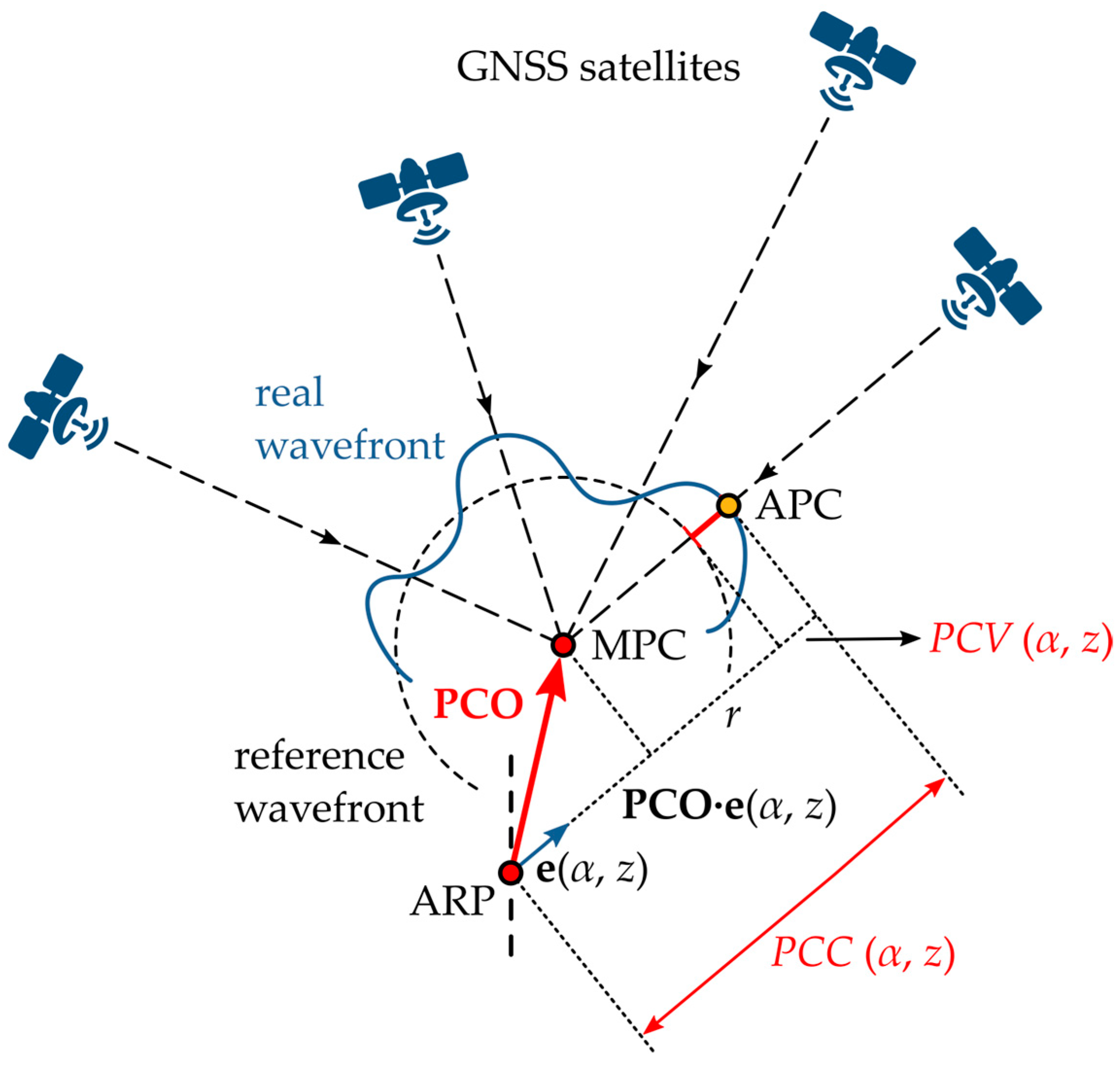
29], the PCC is arbitrarily divided into the phase center offset (PCO) vector and the azimuth- and elevation-angle-dependent phase center variation (PCV). To further explain these quantities, several key antenna-related points, vectors, and scalars, depicted in
Figure 1 and only briefly mentioned in the previous section,
Section 1, must be clarified:
The antenna reference point (ARP) is defined by the IGS as the intersection of the antenna vertical symmetry axis and its bottom plane;
The mean phase center (MPC) is an arbitrary point chosen in such a way that the PCVs are smallest;
The
vector is the line-of-sight unit vector from the receiver to the satellite
i given by:
where
and
are the azimuth and zenith angle of the satellite in the antenna frame (AF);
The scalar is a constant part equal in all directions that can be geometrically interpreted as the radius of the perfect, i.e., ideal, phase wavefront.
To summarize, the receiver antenna PCO is a vector from the ARP to the MPC. The PCV is the direction-dependent distance between the actual phase center (APC) and the reference wavefront. The PCCs are defined in the AF, i.e., an antenna-fixed 3D left-handed coordinate system. The origin of the coordinate system is the ARP. The z-axis of the coordinate system is aligned with the antenna vertical symmetry axis; the x-axis is perpendicular to the z-axis and aligned with the antenna north reference point (NRP). The coordinate system’s y-axis completes the left-handed system. If the antenna is set at the station, assuming it is levelled and correctly orientated (NRP directed to the North), the AF is aligned with the local North-East-Up (NEU) topocentric frame (TF).
Following the IGS convention, the geometric term
from Equation (1) can be expanded as:
where
is the position of the satellite at signal emission time and
is the position of the receiver antenna ARP at signal reception time. Combining Equations (1) and (3), by omitting satellite antenna corrections, the total receiver antenna PCC as a function of PCO and PCV is:
The constant parameter
, contained in Equation (4), is denoted as the datum parameter and is present due to the relative character of GNSS observations, i.e., because with GNSS, only one-way pseudo-ranges can be measured. This parameter does not affect the position estimates and is fully absorbed into the receiver clock error [
9,
12,
39,
47].
By analyzing Equation (4), it is evident that a set of PCC values can be transformed to any PCO vector and PCV set. Therefore, this problem of PCC to PCO/PCV separation has one degree of freedom that must be resolved [
9,
39,
48]. That rank deficiency is contained in the datum parameter
. To not deform the resulting PCV pattern, the PCO/PCV separation must be solved using minimum constraints, i.e., only the parameter
is fixed. The most common approach to solving this rank deficiency is by fixing the PCV at zenith to zero, i.e., the zero-zenith constraint formulated as [
13,
41,
48]:
Therefore, the PCC to PCO and PCV separation is conducted in a single least-squares (LSQ) adjustment using the constrained Gauss–Markov model (GMM) [
49,
50]. The functional model of the LSQ adjustment is based on Equation (4), whereas the adjustment condition can be mathematically expressed as:
The defined adjustment conditions will result with such a PCO vector for which the sum of squared PCVs will be minimal, and, simultaneously, the PCV at zenith will be zero.
2.2. Antenna Calibration System at LMMT
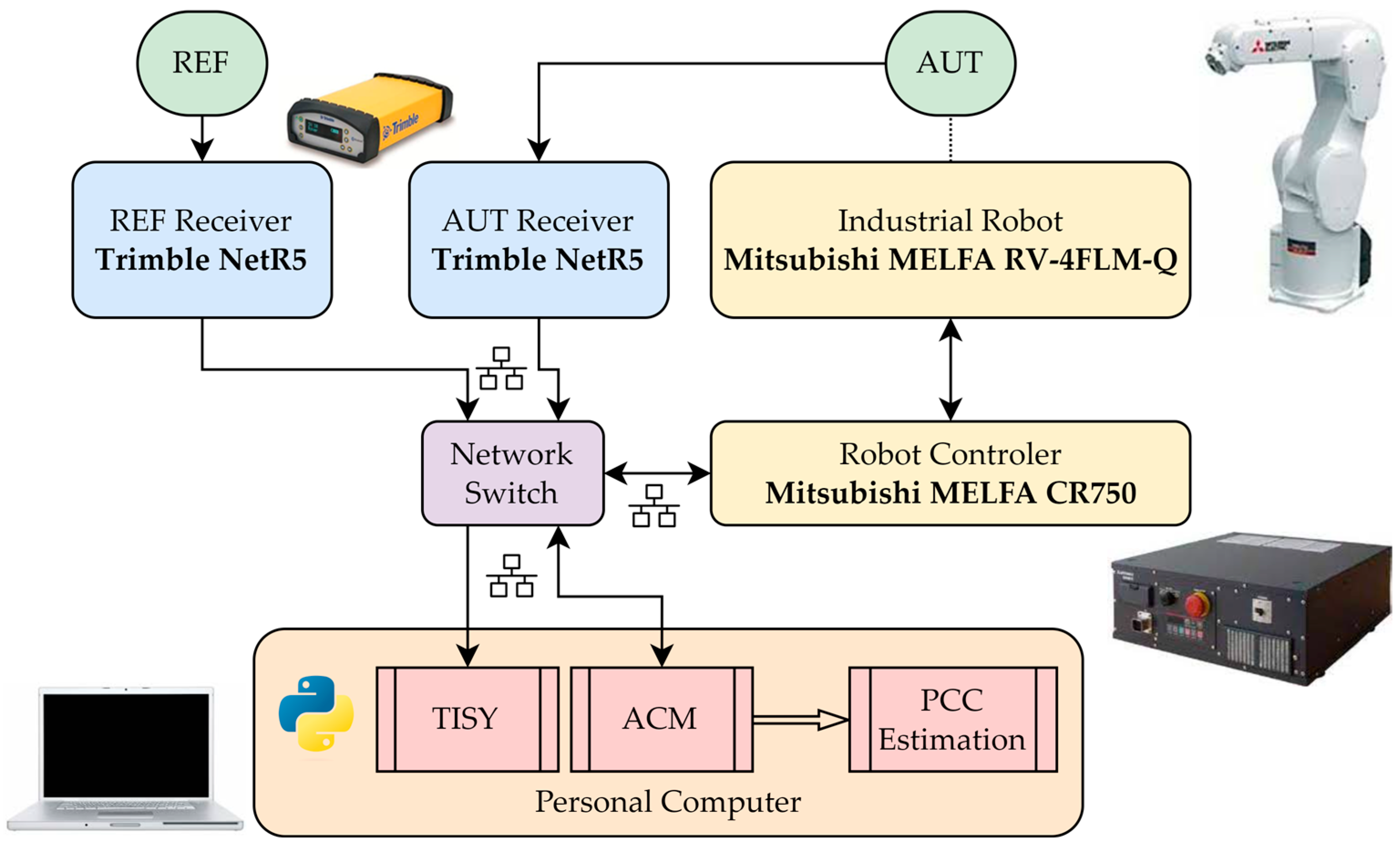
The GNSS receiver antenna calibration system developed at LMMT in the Faculty of Geodesy, University of Zagreb, can be generally divided into two distinct parts: hardware and software. A conceptual representation of the system is depicted in
Figure 2. Hardware wise, the calibration system consists of the following parts:
Industrial robot Mitsubishi MELFA RV-4FLM-Q;
Robot controller Mitsubishi MELFA CR750;
GNSS receiver antennas (REF and AUT);
GNSS receivers (two Trimble NetR5);
Personal computer;
Network switch;
Required robot, antenna, and receiver wiring.
The main software modules of the calibration system at LMMT, all written in Python, are:
To uniformly sample the entire upper-antenna hemisphere, the calibration system at LMMT employs a si
x-axis industrial robot Mitsubishi MELFA RV-4FLM-Q (Mitsubishi Electric Corporation, Tokyo, Japan). It is a vertical structure, multiple-joint-type robot arm with six degrees of freedom and a rated load of 4 kg [
51]. The Mitsubishi MELFA CR750 robot controller is connected to a personal computer (laptop) via an Ethernet cable. Two-way communication between the computer and the robot controller is handled over the TCP/IP protocol. During calibration, each of the antennas (REF and AUT) is connected to the same type of receiver, i.e., a reference-station-grade Trimble NetR5 GNSS receiver (Trimble Inc., Westminster, CO, USA). A standard network switch is used to connect all hardware devices to a local Ethernet network. The antenna calibration field at LMMT consists of two concrete pillars at a mutual distance of 5 m, thus forming a short baseline that is needed for calibration. The pillars are part of the Calibration Baseline of the Faculty of Geodesy of the University of Zagreb [
52].
During antenna calibration, the custom-made ACM reads the calibration parameters and generates a random sequence of antenna orientations (rotations and tilts) to place the AUT. Afterwards, for every antenna orientation, all six robot joint values are calculated and individually sent to the robot controller. When the robot places the antenna at the given attitude, feedback containing current robot joint values is sent to the ACM. The beginning and end of every antenna orientation are timestamped with GPS time so, in later postprocessing, the registered carrier phase observations can be temporally filtered. Parallel to antenna calibration, i.e., the ACM execution, the personal computer’s internal clock is software-wise synchronized to GPS time by simultaneously running TISY. For time synchronization, the 1PPS (one pulse-per-second) signal and the associated TimeTag message, both output by the REF receiver, are used. With such a synchronization approach, the computer’s clock is disciplined and aligned to GPS time with millisecond accuracy. After the calibration is completed, GNSS data on both receivers are preprocessed before final PCC modelling is conducted using the PCC estimation module.
2.3. Antenna Calibration Methodology
At LMMT, during antenna calibration, the industrial robot precisely rotates and tilts the AUT into a total number of 2088 different antenna orientations in the TF. Thereby, the antenna is rotated by an azimuthal increment of 5° in the
interval and tilted by an equal zenithal increment of 5° in the
interval. Positive tilts are defined when the antenna NRP is tilted below and negative when it is above the horizon with respect to the rotation point. The initial antenna position is such that the AF is aligned with the TF. The
a priori nominal mean L1 and L2 MPC is chosen as the antenna rotation point, i.e., as an antenna fixed point in space during calibration. The horizontal distance between the REF antenna ARP and the rotation point is approx. 5 m. Such a short baseline enables the subsequent elimination of the majority of GNSS errors, primarily the signal propagation errors (ionospheric and tropospheric delays) and the satellite orbit error [
4]. At every individual AUT orientation, the antenna is kept stationary for 2.5 s. Afterwards, the robot moves the AUT to the next orientation with an average robot travel time of 1 s. Given the total number of antenna orientations and the orientation timing parameters, a standard calibration at LMMT lasts approx. 2 h. Furthermore, during calibration, 10 Hz GNSS carrier phase observations are registered by both receivers (REF and AUT). The registered raw carrier phase observations, antenna orientation timing data, and the antenna attitude data are the results of field calibration activities and the basis of PCC estimation in the subsequent data processing stage.
Generally, data processing within the PCC estimation software module can be divided into two main steps. Firstly, the registered raw carrier phase observations are preprocessed and prepared for the subsequent PCC LSQ modelling, PCC to PCO/PCV transformation, and, finally, ANTEX file export. At its core, the new calibration system at LMMT is based on the approach of time-differenced double-difference (DD), i.e., triple-difference (TD), carrier phase observations [
53], similar to Hu et al. [
8] and Willi et al. [
10,
16]. The main goal of phase differencing is a reduction in or the full elimination of GNSS error sources. It is emphasized that, with such a processing approach, the strong spatial and temporal signal correlation is exploited, as will be further explained below.
Initially, based on the raw carrier phase observations registered by the REF and AUT receivers, the between-receiver single differences (SDs) for satellite
at epoch
are formed:
where
and
are raw GNSS carrier phase observations for the REF and AUT stations according to Equation (1) but with shorter R (REF) and T (AUT) notations. On a 5 m long short baseline, GNSS signals are strongly spatially correlated, i.e., the tropospheric and ionospheric delays practically identically influence both stations, and, therefore, are eliminated in the differencing process. Moreover, the satellite clock error and hardware delay, which are identical for two time-synchronized observations on two different receivers, regardless of the distance between them, are also eliminated. Therefore, combining Equations (1) and (7) produces:
where the subscript “T,R” notation indicates that REF and AUT differences for each parameter are involved.
In this step, the differential geometric term
and the differential PWU
are modelled and removed from the single-difference observation in Equation (8). Thereby, the geometric distances from the satellite to the REF and AUT stations are modelled based on the interpolated satellite position and known station coordinates. Satellite orbits are interpolated at epoch
using IGS rapid SP3 orbit solutions by a 10th order Legendre polynomial [
54,
55]. The PWU effect is modelled according to the equations of Wu et al. [
56]. Thereby, special care must be taken to determine the AUT and REF antenna orientation with respect to the Earth-Centered Earth-Fixed (ECEF) reference frame that the satellite orbits are defined in, e.g., ITRF2020.
Additionally, by comparing the time of epoch with the antenna orientation timing data, every individual SD value is labeled with the unique antenna orientation identifier. The main goal of this step is to discard the phase observations that have been registered during robot movements. Furthermore, based on the known AUT attitude in the TF, the azimuth and zenith angles of the satellite are transformed into the AF.
Introducing an additional satellite
, two corrected single-difference carrier phase observations are further differenced to form the well-known DD carrier phase observations:
By double-differencing, the constant part of both single differences is removed, i.e., the receiver clock error and hardware delay:
It is evident that the double-difference carrier phase observation contains only the differential integer ambiguity , the differential multipath , and the PCC values of the REF and AUT antennas for the and satellites plus the differential phase noise.
Finally, TDs are formed by applying time differences to the DD carrier phase observations from Equation (10) as:
where the operator
is used to indicate the time difference of epochs
and
. It is also important to note that the method of calculating time differences is key. For antenna calibration, TDs must be formed between two different time-neighboring antenna orientations. Therefore,
and
do not simply refer to two time-adjacent epochs but refer to two epochs in two different time-adjacent AUT orientations. Thus, depending on the calibration timing parameters, the time difference between
and
can be up to 5 s.
Due to the strong temporal correlation of GNSS signals, all parameters that are constant over a specific amount of time will be eliminated in the TDs. If no cycle slips occur, the DD ambiguity
is equal in epochs
and
. Cycle slip will appear as integer wavelength value jumps in the TD time plot and can easily be removed through simple outlier detection [
10]. If the time differences between the epochs
and
is sufficiently small (up to 5 s), the multipath effect does not change [
57] and will also be eliminated in the differencing process. Furthermore, because the REF antenna is stationary during calibration, the GNSS satellite very slowly changes its position in the AF. Thus, from the REF antenna’s point of view, it is valid:
Therefore, by forming TDs on a short baseline and in a short time interval, the REF antenna PCC is fully eliminated, which truly leads to an absolute calibration of the AUT. Incorporating these simplifications into Equation (11), the final equation is derived:
The TD carrier phase observation contains only the AUT PCCs and the differential phase noise. This equation is the basis of the functional model of LSQ adjustment and PCC estimation.
Because the PCCs of a receiver antenna are defined on the entire upper-antenna hemisphere, for expressing the preprocessed set of TD carrier phase observations with a unique function, spherical harmonics (SHs) are best suited. Therefore, PCCs are parametrized by SH expansion and, at LMMT, the degree
and order
are used. The fundamental equation of SH expansion is given by:
where
is the fully normalized Legendre function [
58],
and
are the SH coefficients, and
and
are the azimuth and zenith angles in the AF. For the SH resolution
, a total of 91 SH coefficients are defined. Therefore, to fit an SH expansion to a set of data on a sphere (or part of a sphere), the unknown SH coefficients must be determined in an LSQ sense. Integrating Equation (14) into Equation (13), a fundamental observation equation of the functional model of LSQ adjustment is defined:
The functional model given by Equation (15) is linear with respect to the unknowns, i.e., the SH coefficients
and
. Therefore, the linearization of the model in the vicinity of the solution is not necessary, and the solution converges in the first adjustment iteration. However, because only observations in the upper-antenna hemisphere are available for SH expansion, this functional model is weakly conditioned, and its restriction is needed [
9,
10]. All SH coefficients that represent anti-symmetry of the two antenna hemispheres and have an odd index sum are restricted to zero. Moreover, the absolute term
cannot be determined and is also restricted to zero. Therefore, to determine the SH coefficients in an LSQ sense and to fulfill the set conditions, the constrained GMM is applied [
9,
49,
50].
After solving for the unknowns, i.e., the SH coefficients, the PCCs of the AUT are calculated for the entire antenna upper hemisphere according to Equation (14) in a regular grid for
and
, with an azimuthal and zenithal increment of 5°. Such grid definition is in accordance with common ANTEX entries. The PCCs of the AUT are transformed to the PCO vector and PCVs according to Equations (5) and (6) and the method elaborated in
Section 2.1. Finally, the resulting PCO vector and PCVs are exported to ANTEX format.
2.4. PCC Comparison Methodology
Because a unique PCO and PCV set cannot be determined and a datum definition is required during PCC to PCO/PCV transformation, as previously elaborated in
Section 2.1, the comparison of different antenna calibration results of the same antenna must be conducted exclusively at the PCC level. To be able to correctly calculate the difference pattern
of two PCC sets,
and
, they firstly have to be brought to a common PCO vector and datum [
9,
41,
48,
59]. Therefore, the second PCC set,
, can be transformed to the PCO vector and datum of the first set
by:
where
is the PCV set transformed to the PCO vector and datum of the first PCC set
and is obtained by:
where
is the PCO difference vector and
is the difference in the
z-axis components of both PCO vectors.
After transformation to common PCO vector and datum, the difference pattern of the PCC sets of interest is calculated as:
Thus, the gained PCC difference pattern
is the basis for calculating quantitative scalar measures of the difference between two antenna calibration results. Similar to the proposal of Schön and Kersten [
59] and Kersten at al. [
41], the following scalar measures for PCC comparison are defined:
Minimum ΔPCC—minimal value of PCC differences;
Maximum ΔPCC—maximal value of PCC differences;
Root-mean-square (RMS) deviation of the ΔPCC—average quadratic deviation of PCC differences;
Range of the ΔPCC—the difference between the maximum and minimum PCC differences;
Interquartile range (IQR) of the ΔPCC—measure of the spread of the middle 50% of PCC differences.
3. Results and Discussion
To initially test the receiver antenna absolute field calibration system developed at LMMT of the Faculty of Geodesy at the University of Zagreb in Croatia, to examine the repeatability of individual calibrations of the same antenna, and to validate the LMMT calibration results with independent calibrations obtained by Geo++ GmbH, an IGS-approved institution, from late April to mid-June of 2023, four individual absolute calibrations of the same Trimble Zephyr 2 Geodetic antenna (TRM57971.00 NONE, S/N: 30739001) were carried out. In this article, preliminary calibration results for the GPS L1 frequency (G01) are presented and elaborated. Information on the conducted antenna calibration campaigns is summarized in
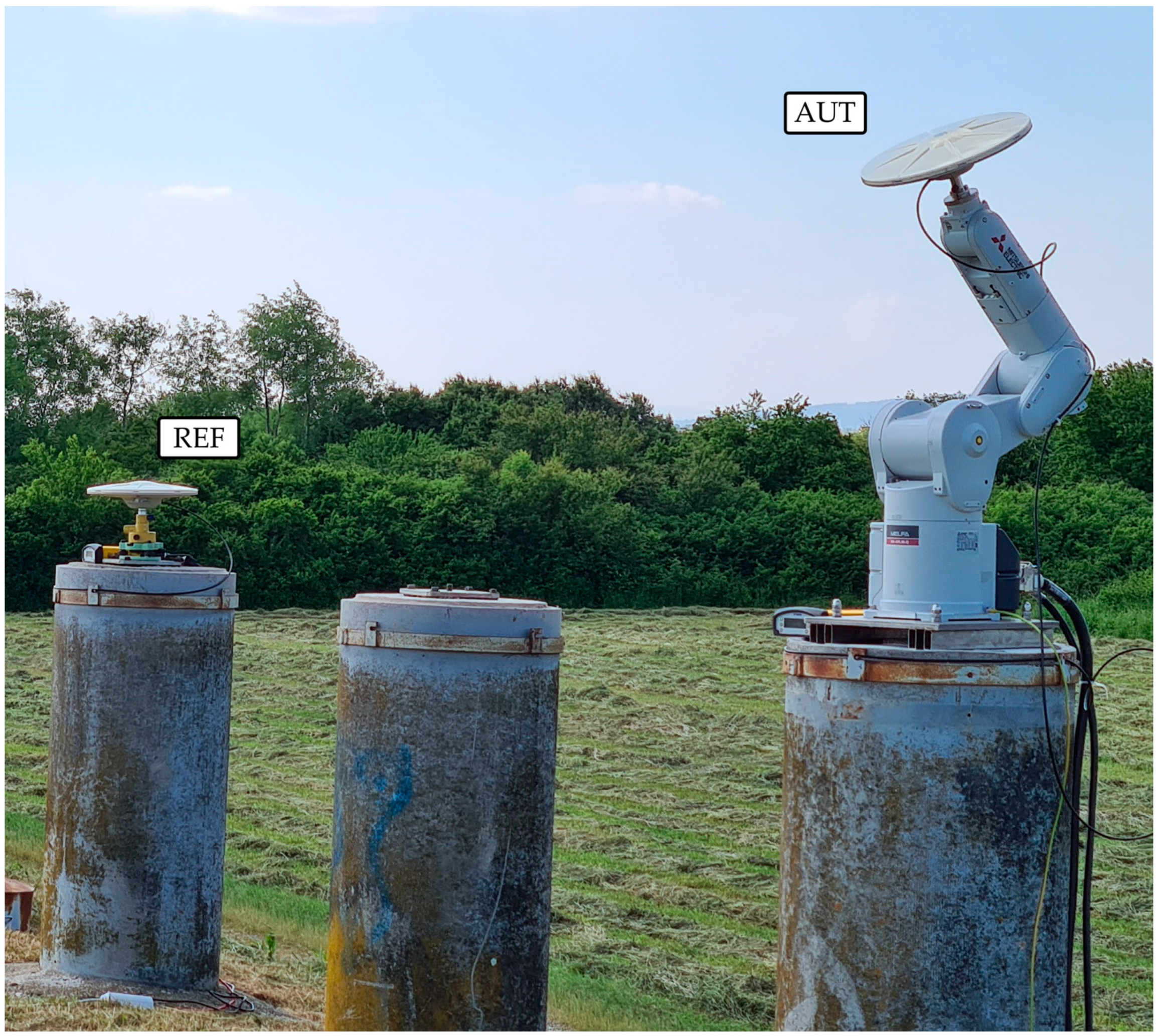
Table 1. Across all four calibrations, the same type of reference-station-grade GNSS receivers (Trimble NetR5) on both REF and AUT stations with equal settings were used. Furthermore, another antenna of the same type, TRM57971.00 NONE (S/N: 30734472), was used as the REF antenna. In
Figure 3, the antenna calibration system set-up at LMMT, previously elaborated in
Section 2.2, is depicted. It is also noted that across all four campaigns, satellite geometries were different, and due to the different number of satellites, significantly different observation numbers (TDs) were obtained.
Based on the results of four individual calibrations, the quantitative measure on the repeatability of antenna calibration at LMMT is estimated. Furthermore, the antenna in question was considered on 5 August 2022, individually calibrated at Geo++ GmbH in Germany. Thus, the validation and comparison of the LMMT calibration results with different independent institutions are possible. Such analysis enables an external independent accuracy validation of the calibration system at LMMT.
3.1. PCC Estimation Results
According to the elaborated methodology of antenna PCC LSQ estimation, calibration results for antenna TRM57971.00 NONE (S/N: 30739001) of four conducted calibration campaigns are obtained. In
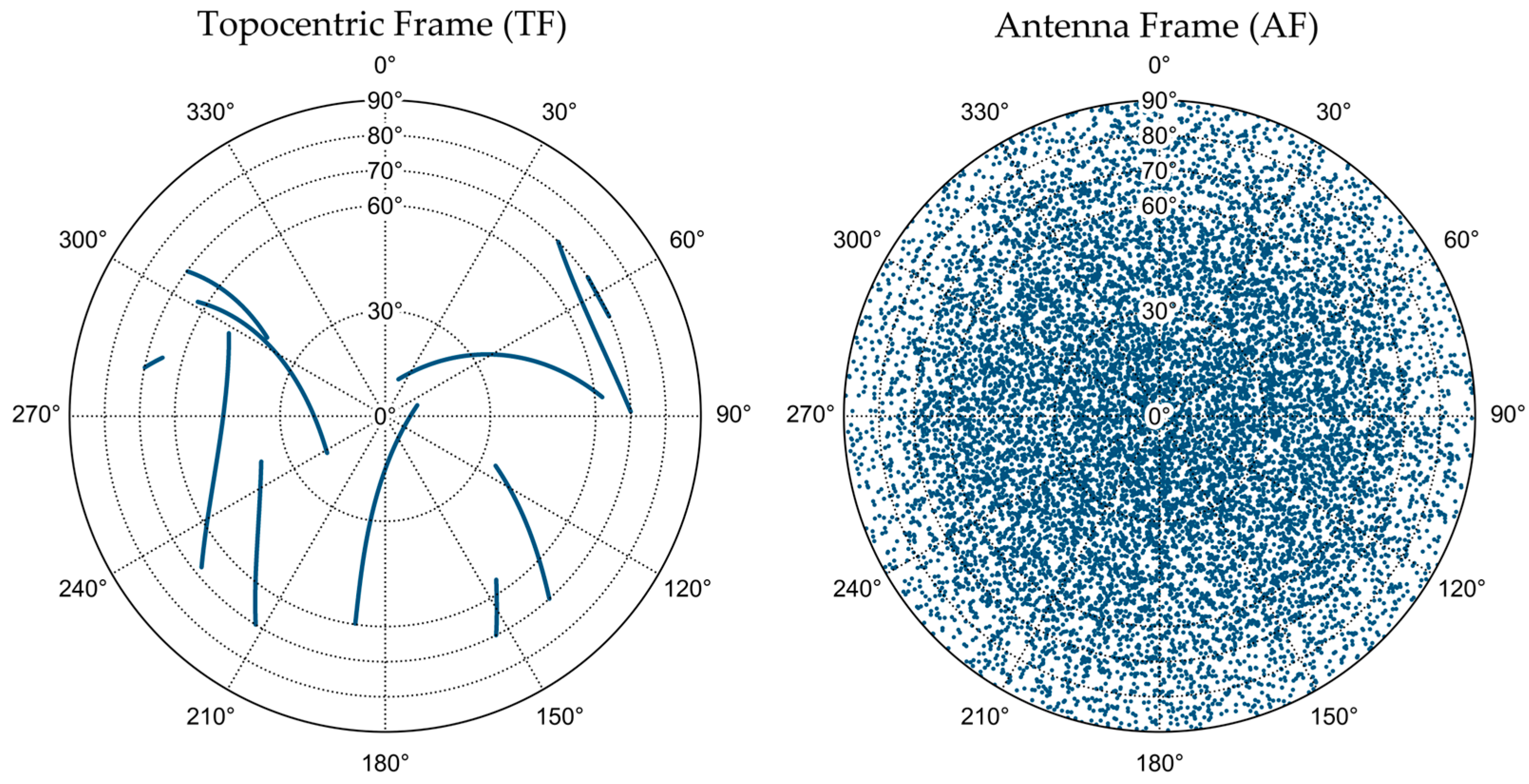
Figure 4, the satellite azimuth and zenith angle plots (sky-plots) for calibration campaign 4 (DoY 167) are presented. The left sky-plot refers to the TF, i.e., a static, levelled, and North-orientated antenna, whereas the right plot to the AF during calibration when the antenna is, according to the LMMT orientation method, rotated and tilted by the industrial robot. From the TF plot, it can be seen that 11 GPS satellites were available during calibration campaign 4. It is evident that rotations and tilts of the AUT have led to an even and homogeneous observation coverage of the entire antenna hemisphere. However, a lower density of observations at low elevations (<20° of elevation) is noticeable. This is a direct consequence of an elevation mask of 20° during antenna calibration and the antenna orientation method at LMMT.
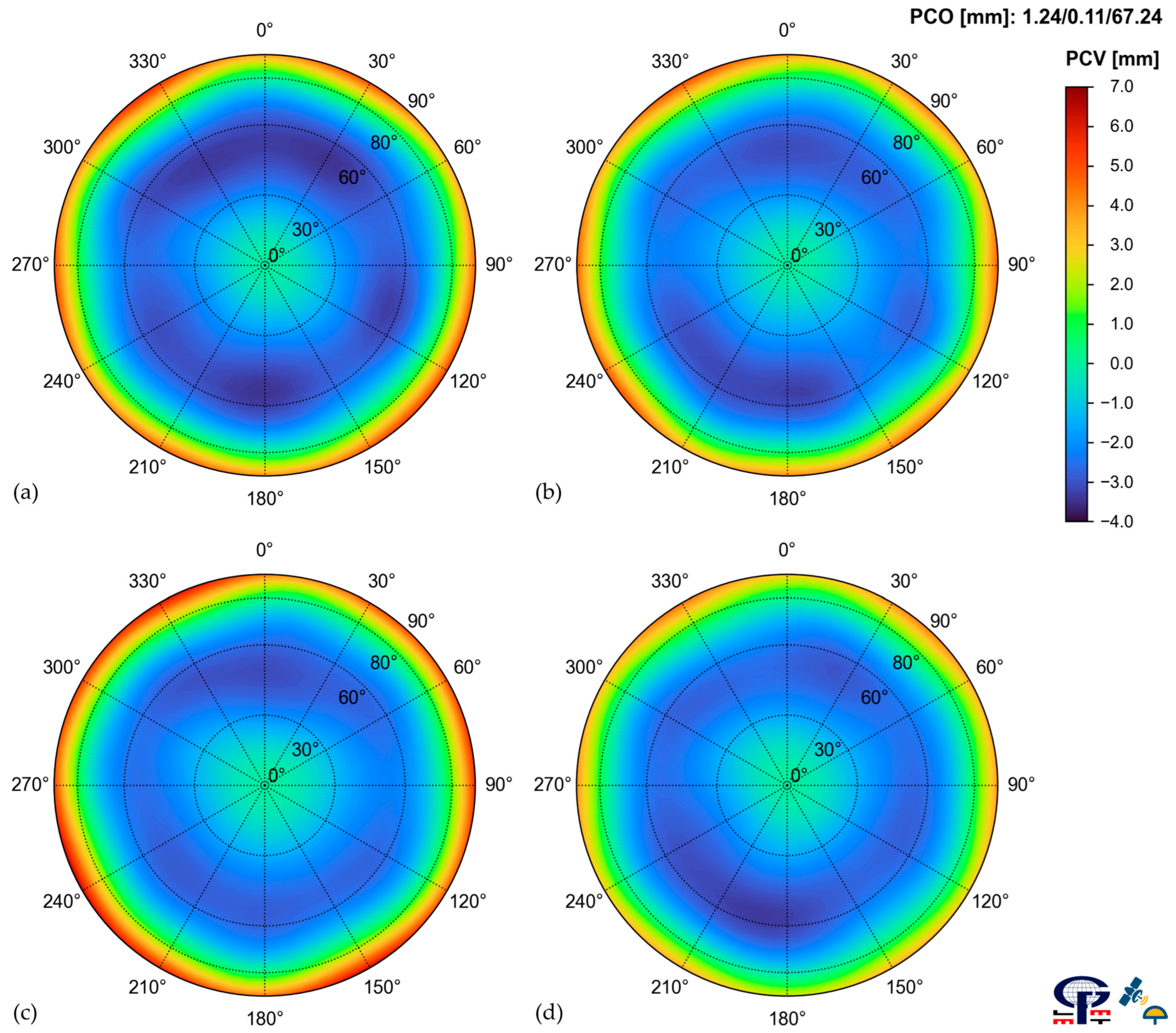
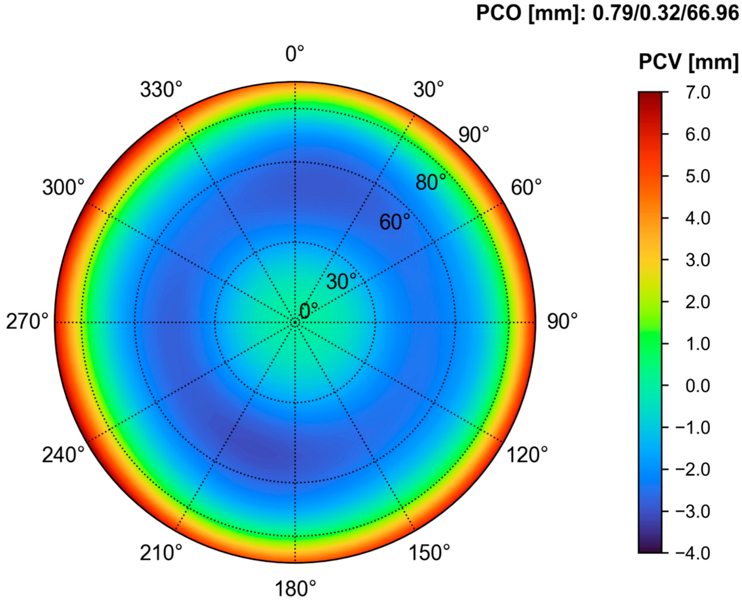
The estimated PCOs for GPS L1 frequency (G01), for every individual calibration campaign of antenna TRM57971.00 NONE (S/N: 30739001), are presented in
Table 2. Vary small PCO differences are obtained with PCO standard deviations in the North/East/Up directions of 0.20/0.05/0.40 mm. Therefore, a submillimeter PCO precision was gained from four independent absolute calibrations for the investigated GNSS antenna.
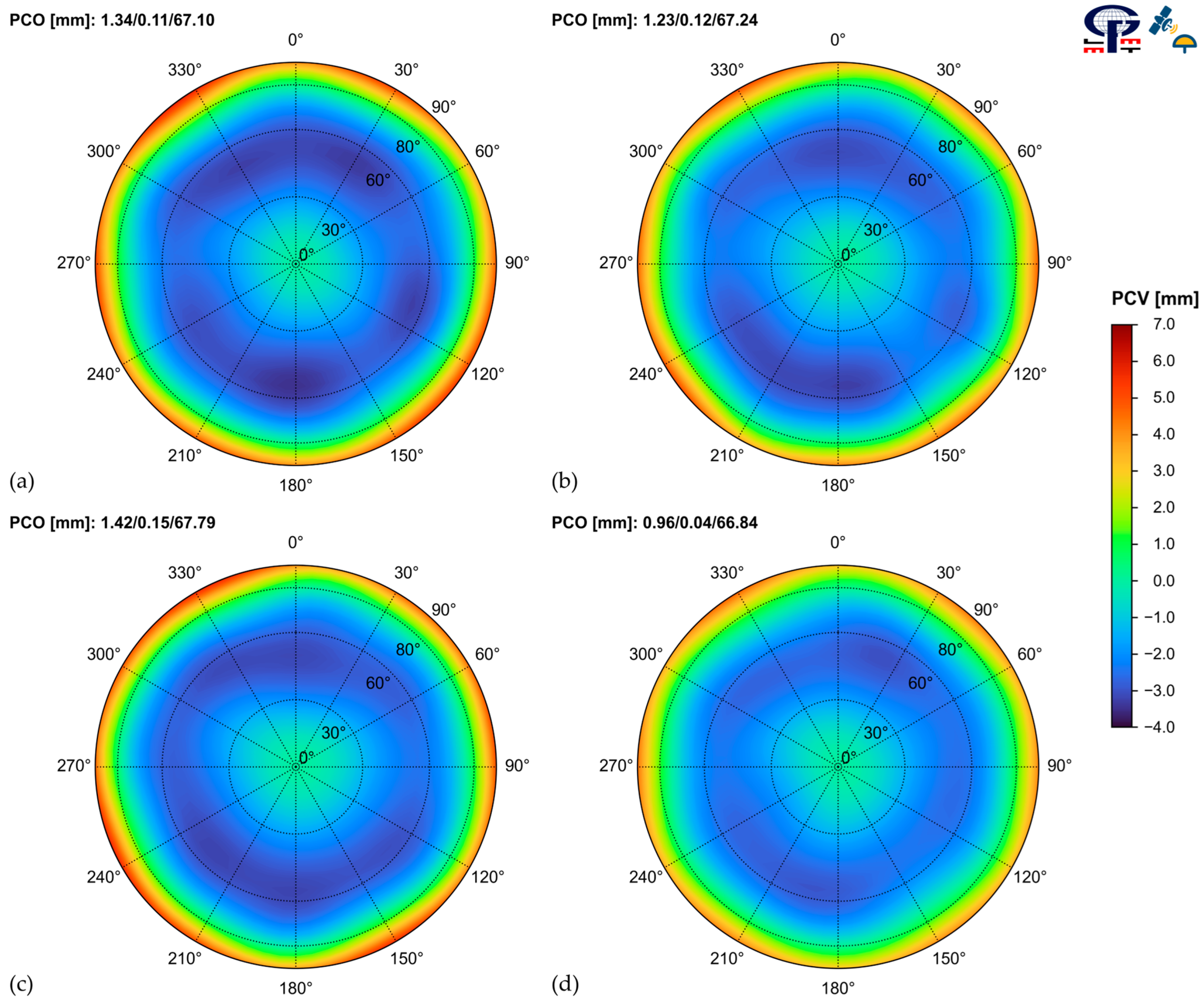
The estimated PCVs for GPS L1 frequency (G01), for every individual calibration campaign of antenna TRM57971.00 NONE (S/N: 30739001), are depicted in
Figure 5. All PCV patterns, as expected, show high zenith-dependent variations, e.g., from –3.5 mm (campaign 1) to +5.8 mm (campaign 3). However, small azimuth-dependent variations are noticeable. In summary, calibration results, across all calibration campaigns, show similar PCV behavior over the entire antenna hemisphere.
3.2. Repeatability of PCC Estimation
To adequately compare the obtained calibration results of the investigated antenna TRM57971.00 NONE (S/N: 30739001) and to examine the repeatability of individual absolute calibrations at LMMT, all four estimated PCC models must firstly be brought to a common PCO vector and datum (
Section 2.4). Therefore, based on the estimated PCO vectors (
Table 2), the mean PCO vector for GPS L1 frequency, across all four calibration campaigns, is calculated (
Table 3). According to the methodology elaborated in
Section 2.4, the calibration results of all four calibration campaigns are subsequently transformed to this mean PCO. The obtained transformed PCVs are depicted in
Figure 6.
Based on the four obtained PCO- and datum-aligned PCC antenna patterns, the following quantitative pattern-based scaler measures are calculated and shown in
Table 4:
Maximal range—the maximal of all range values calculated at every PCC azimuth- and zenith-grid node;
Average range—the average of all range values calculated at every PCC azimuth- and zenith-grid node;
Average standard deviation—the average of all standard deviation values calculated at every PCC azimuth- and zenith-grid node.
Furthermore, because during the majority of GNSS applications, an elevation mask of minimally 10° is common and standard practice, a 10° elevation-reduced antenna hemisphere analysis is justified. Therefore, to further analyze the calibration differences at low elevations, the previously elaborated quantitative scalar measures are also calculated with an elevation-reduced antenna hemisphere (
Table 4).
From the obtained results, it can be seen that the highest difference between multiple calibrations of the TRM57971.00 NONE (S/N: 30739001) antenna, taking the entire antenna hemisphere in account, is 3.41 mm. The average difference between multiple calibrations is 0.55 mm, and the average standard deviation is 0.24 mm. However, if a 10° elevation-reduced antenna hemisphere is considered, the maximal difference between the individual calibrations drops down to 2.03 mm, whereas the average difference is 0.42 mm, and the average standard deviation is 0.19 mm. Therefore, significantly higher differences between the four conducted individual antenna calibration results are found at low antenna elevations.
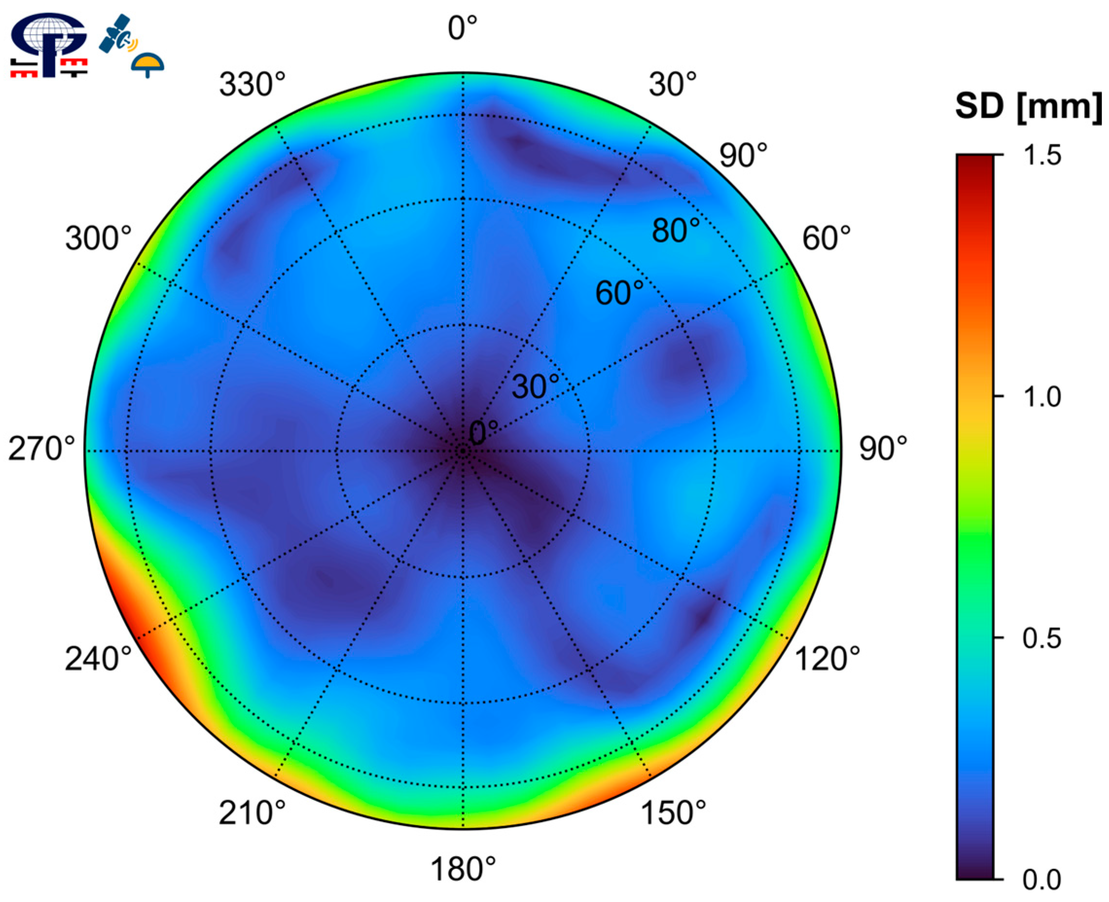
Furthermore, to gain a visual representation of the differences between the four calibration campaign results of the investigated TRM57971.00 NONE (S/N: 30739001) antenna, the standard deviation over the entire antenna hemisphere is plotted and depicted in
Figure 7.
From the previous standard deviation plot (
Figure 7), it can be concluded that the precision of individual calibrations for the entire antenna hemisphere is below 1 mm, except for the three low-elevation regions at
, where the standard deviation reaches 1.5 mm (
). If only the elevation-reduced antenna hemisphere is considered, it can be concluded that the precision of individual calibrations is below 0.5 mm.
To summarize, if the full antenna hemisphere is considered, the precision of individual calibrations at LMMT for the TRM57971.00 NONE (S/N: 30739001) antenna and for GPS L1 (G01) frequency is 0.24 mm, with an average difference between the multiple calibration results of 0.55 mm. However, if a 10° elevation-reduced antenna hemisphere is considered, the precision of multiple calibrations is 0.19 mm, with an average difference between multiple calibrations of 0.42 mm. It is evident that higher differences exist at low antenna elevations. It must be noted that, due to the datum definition of initial PCC calibration results, i.e., the zero-zenith constraint, the highest differences between calibrations would be expected precisely at the lowest antenna elevations. All obtained results achieved a submillimeter repeatability of individual absolute antenna calibrations at LMMT.
3.3. Validation of PCCs
LMMT receiver antenna individual absolute calibration results for the TRM57971.00 NONE (S/N: 30739001) antenna and the GPS L1 (G01) frequency were validated through comparison with independent individual calibration results obtained by Geo++ GmbH in Germany. Geo+ GmbH is one of the IGS-approved institutions to provide absolute antenna calibrations. The investigated antenna was calibrated by Geo++ GmbH on 5 August 2022. The following figure,
Figure 8, shows the Geo++ GmbH calibration results (PCO and PVC) for TRM57971.00 NONE (S/N: 30739001) and G01 frequency. It is noted that the PCV color scale is equal to the color scales in
Figure 5 and
Figure 6.
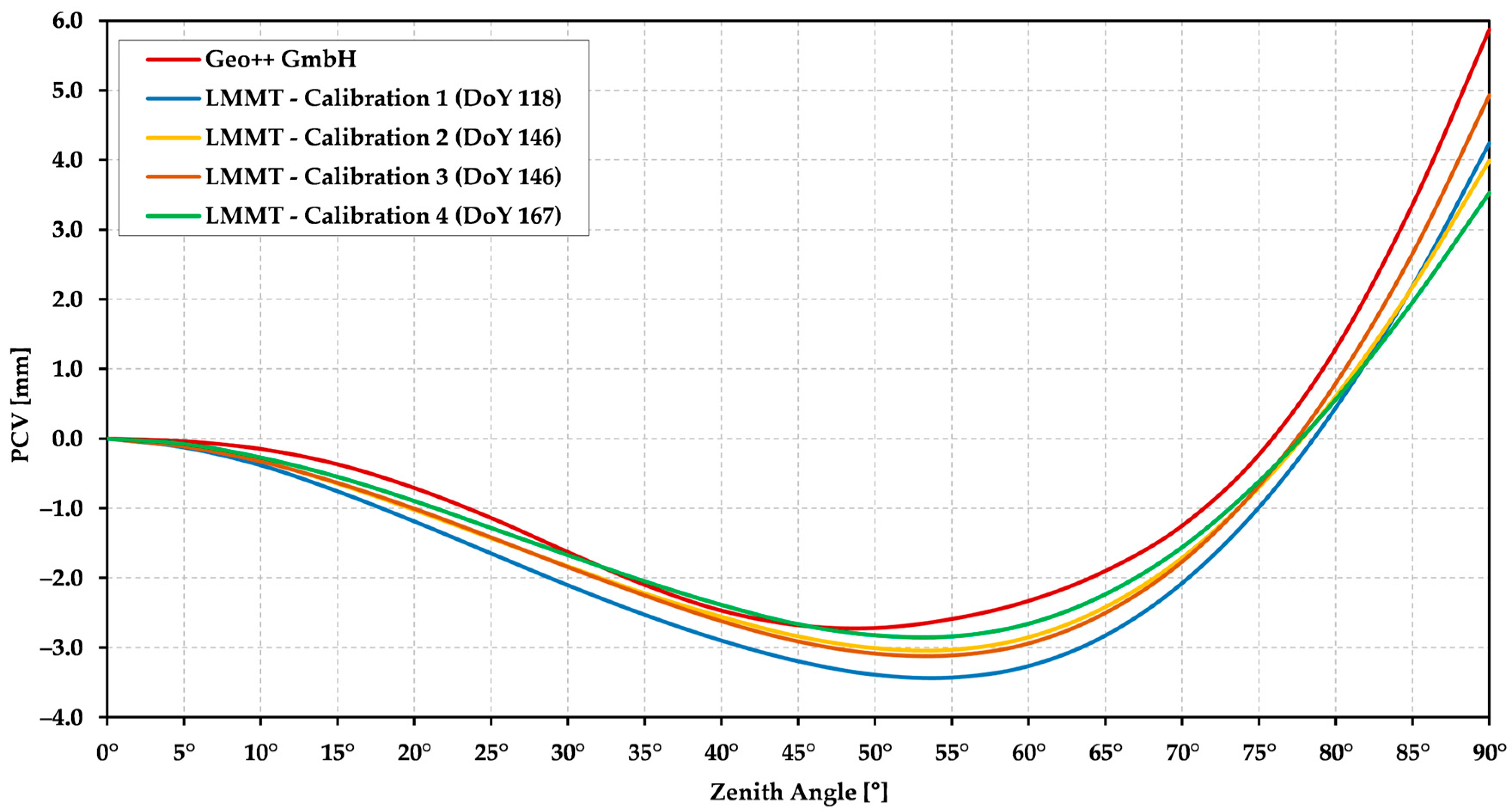
The accuracy of LMMT calibrations was determined by taking the Geo++ GmbH calibration results as reference values. Therefore, LMMT calibration results for every calibration campaign were initially, according to the method elaborated in
Section 2.4, PCO- and datum-wise transformed to the Geo++ GmbH PCO vector. To further visualize the Geo++ GmbH and LMMT calibration results, the zenith-only-dependent PCV patterns (NOAZI ANTEX entry) are plotted and shown in
Figure 9. Generally, lower LMMT PCV values, across all calibration campaigns, with respect to Geo++ GmbH results, are noticeable.
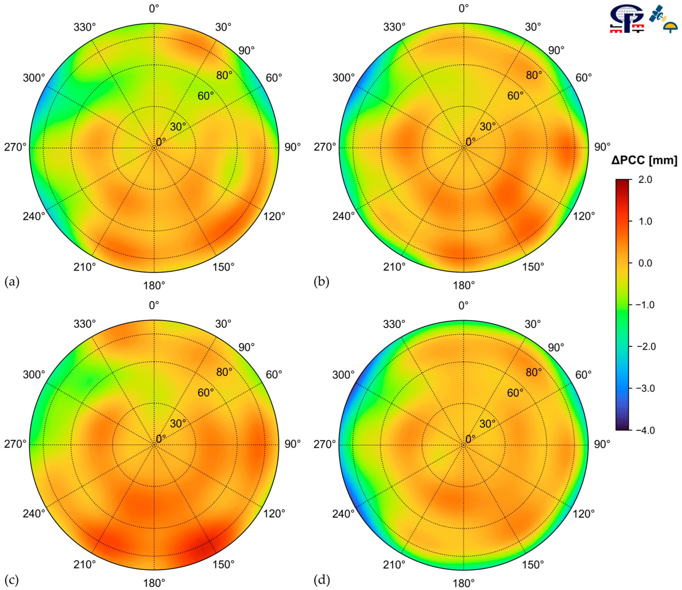
Following the PCO- and datum-wise transformation of LMMT calibration results to the reference Geo++ GmbH PCO vector, according to Equation (18), the PCC difference patterns
, across all calibration campaigns, were calculated and are visualized in
Figure 10. They are the basis for LMMT antenna calibration accuracy validation. Through simple visual inspection of the gained PCC difference patterns, it is evident that values around zero prevail with several extreme regions mainly located in lower elevations. Also, it is evident that negative values of
occur more often.
To obtain a quantitative estimate of the accuracy of LMMT calibration results, according to considerations in
Section 2.4, scalar measures based on the acquired PCC difference patterns were calculated and are campaign-wise given in
Table 5. Therefore,
Table 5 is somewhat of a numerical summary of the
differences depicted in
Figure 10. Again, according to previous elaboration, quantitative scalar measures were calculated considering the full antenna hemisphere and the 10° elevation-reduced antenna hemisphere.
Considering the full antenna hemisphere, the range values of the Geo++ GmbH and LMMT PCC differences (), across all calibration campaigns, are from 3.16 mm to 4.29 mm. The middle half of the PCC differences (IQR values) is below 0.54 mm, and the RMS values, which quantify the overall agreement of the Geo++ GmbH and LMMT PCC patterns, are below 0.71 mm, with an average RMS of 0.58 mm. However, if only the elevation-reduced antenna hemisphere is considered, the quantitative scalar measures significantly improve across all calibration campaigns. The middle 50% of the PCC differences are below 0.50 mm, and the RMS values are below 0.47 mm, with an average RMS of 0.39 mm. The range values are more consistent and are from 2.39 mm to 2.65 mm.
To summarize, based on the results of four individual absolute calibrations with the new calibration system developed at LMMT for the same GNSS antenna TRM57971.00 NONE (S/N: 30739001) and GPS L1 (G01) frequency, an estimated agreement to within 0.58 mm with accredited Geo++ GmbH calibration results, for the whole antenna hemisphere, has been achieved.
4. Conclusions
The new GNSS receiver antenna calibration system, and the underling calibration method, developed from scratch at the Laboratory for Measurements and Measuring Technique (LMMT) of the Faculty of Geodesy at the University of Zagreb in Croatia, provides meaningful receiver antenna calibration results for GPS L1 frequency.
To evaluate the new antenna calibration system, four individual absolute calibrations of the same Trimble Zephyr 2 Geodetic antenna (TRM57971.00 NONE, S/N: 30739001) were carried out. Based on the gained calibration results, across all calibration campaigns, the quantitative measure on the repeatability of antenna calibrations was estimated. The obtained results show a standard deviation of multiple calibrations of 0.24 mm if the entire antenna hemisphere is considered and a standard deviation of 0.19 mm considering a 10° elevation-reduced antenna hemisphere. Therefore, submillimeter repeatability is achieved for GPS L1 frequency. Furthermore, the obtained LMMT calibration results were compared with Geo++ GmbH results. An estimated agreement to within 0.58 mm in terms of RMS, for the whole antenna hemisphere, and to within 0.39 mm in terms of RMS, for the elevation-reduced antenna hemisphere, was achieved. These results confirm the compatibility of the LMMT GPS L1 antenna calibrations with the calibrations of Geo++ GmbH.
However, all calibration results have consistently shown that significantly worse calibration results are obtained for low antenna elevations (<10°). This issue requires further investigation. A possible source could be a lower density of observations at low antenna elevations (<20° of elevation), as can be seen in
Figure 4. Generally, a GNSS antenna is not designed to receive signals at 0° elevation because, at low elevations, a GNSS antenna has the lowest gain, i.e., its power receiving capabilities are the weakest. Therefore, in the initial step, the antenna orientation method should be revised, whereby greater emphasis to better coverage at lower antenna elevations should be given. Furthermore, the calculated LMMT and Geo++ GmbH PCC difference patterns, across all calibration campaigns, show predominantly negative values. This issue, due to the possibility of a systematic cause, requires further investigation.
Finally, the GNSS receiver antenna calibration system at LMMT continues to be developed and tested. The primary goal is to upgrade the system and to provide multi-frequency and multi-GNSS calibrations to the antenna community. Since the antenna calibration topic is of high interest to the scientific community, a new operational calibration system is highly desirable.


