1. Introduction
Over the last few decades, remote sensing data acquired from interferometric synthetic aperture radars, satellite altimetry, gravity-dedicated satellite missions, and other space geodetic techniques have been used to develop global topographic, bathymetric, ice thickness, and gravitational models. These models have been facilitated in numerous Earth science applications. Since seismic data coverage is still sparse and uneven in many parts of the world, these models have also been used in studies of the Earth’s interior. In global and large-scale regional studies, for instance, the Earth’s external gravitational field derived from orbital perturbations of satellites and (more recently) directly from gravity-dedicated satellite missions helped scientists to better understand the mantle structure that mainly propagates into a long-wavelength geoidal geometry (e.g., [
1,
2,
3,
4,
5,
6,
7,
8,
9,
10,
11]). These satellite missions involved the Challenging Mini-satellite Payload (CHAMP) [
12], the Gravity Recovery and Climate Experiment (GRACE) [
13], the Gravity field and steady-state Ocean Circulation Explorer (GOCE) [
14,
15], and the GRACE Follow-On (GRACE-FO) [
16]. The GOCE provides information about the external gravitational field with a spatial resolution ~80 km (in terms of a half-wavelength) that has further been refined by incorporating available ground-based, air-borne, and sea-borne gravity measurements as well as marine gravity data derived from processing satellite altimetry observables (e.g., [
17]).
In gravimetric studies of the Earth’s interior, gravitational, topographic, bathymetric, and ice thickness models together with additional geophysical and geological information are typically used to investigate the lithospheric structure (e.g., [
18,
19,
20,
21,
22,
23,
24,
25,
26]). To study structures deeper in the mantle, long-wavelength geoidal undulations are more suitable for this purpose [
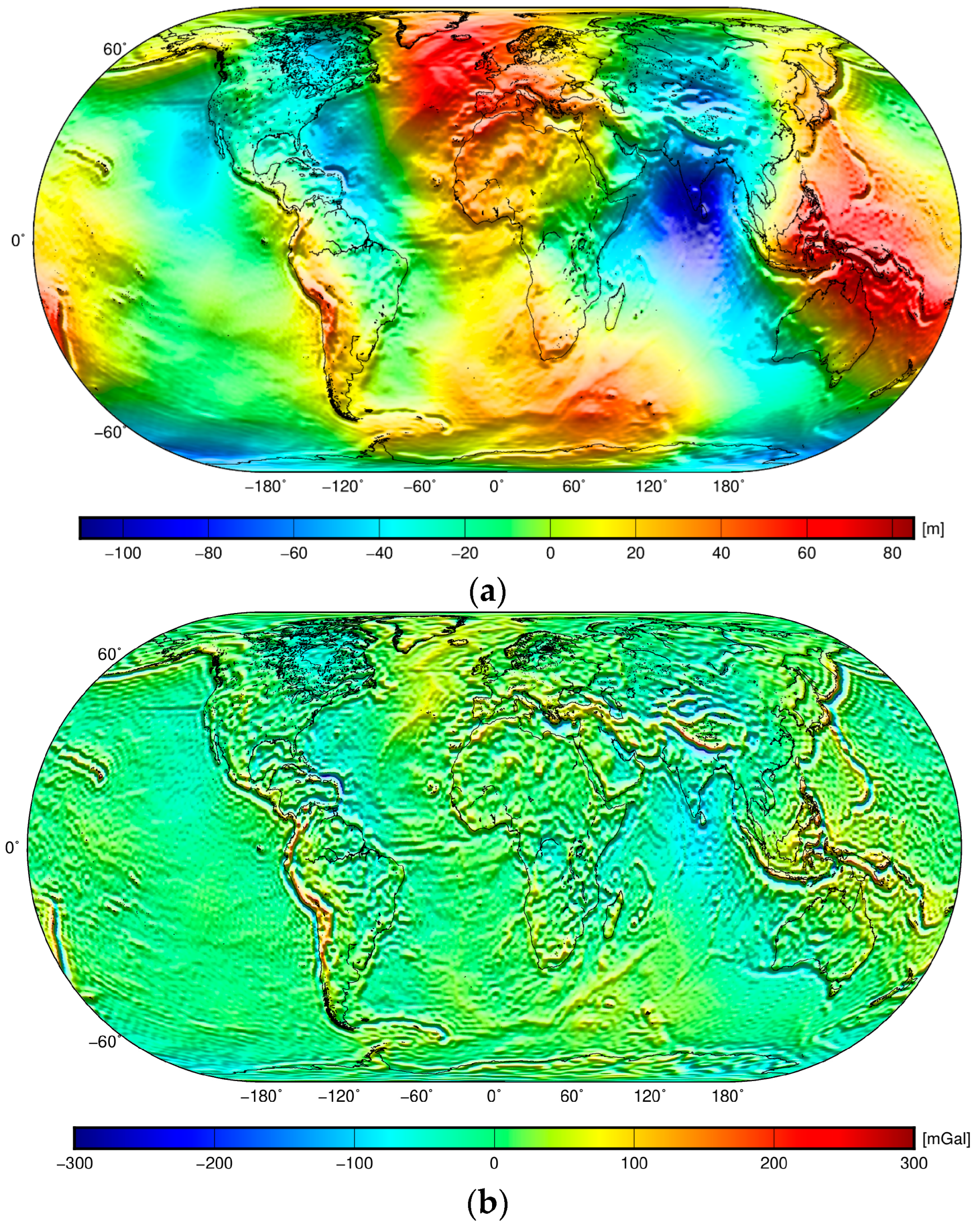
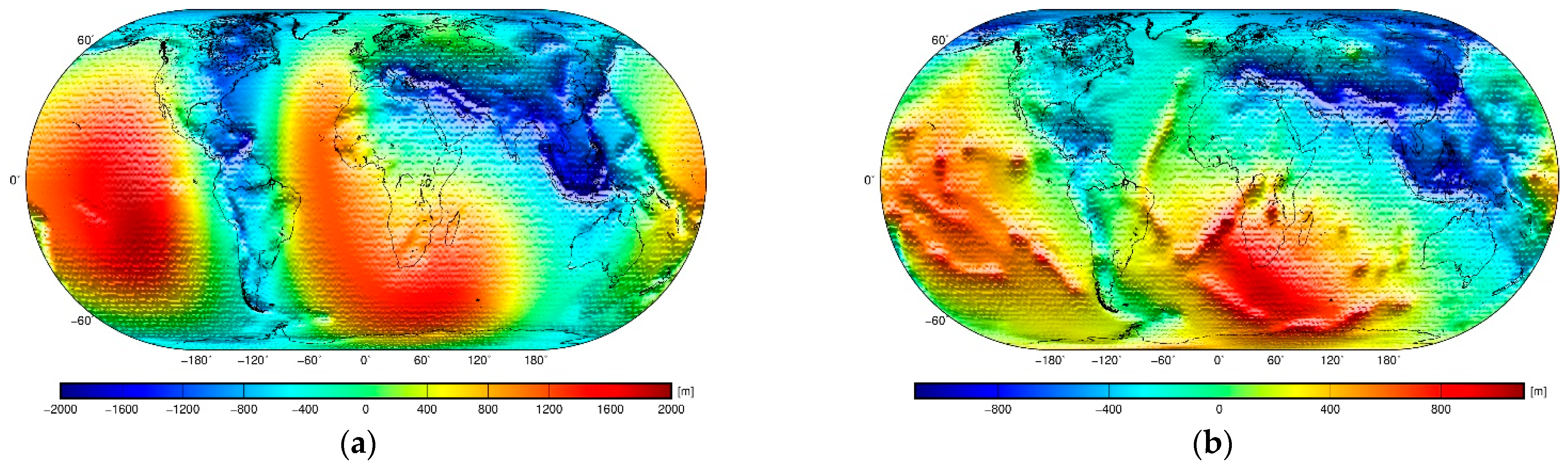
27]. The reason is that a geoidal geometry mainly comprises a long-wavelength signature of the mantle density structure, while a medium-to-higher-frequency part of the gravity spectrum (largely attributed to lithospheric density and geometry) is to some extent filtered out in the geoidal geometry. In contrast, the lithospheric signature (including topographic and ocean floor relief) is better pronounced in the gravity field. This is evident from the global geoid and free-air gravity maps shown in
Figure 1.
As already stated, more detailed features in the geoidal geometry attributed to lithospheric density and geometry variations are to some extent filtered out. Nevertheless, the gravimetric interpretation of the Earth’s mantle density structure (controlled mainly by mantle convection flow) might be improved by applying forward modelling and the subsequent removing of the gravitational signature of lithospheric density and geometry variations in the geoidal geometry. This procedure is applicable only if lithospheric thickness and density models are sufficiently accurate. Alternatively, an approximate method might be used that is based on applying a particular isostatic theory. In addition, methods based on spectral decomposition and filtering techniques have been used to enhance the long-wavelength signature of deeper sources and to suppress random noise in order to enhance real signals (or systematic trends) in gravity field quantities (i.e., potential, gravity, and gravity gradient data).
In global and large-scale regional studies, the CRUST1.0 [
29] and LITHO1.0 [
30] models can be used to compute and remove the gravitational contribution of lithospheric structures. These models were derived from tomographic surveys based on the conversion of seismic wave velocities to rock density values [
31]. Both models, however, have limited accuracy and resolution because a direct relation between seismic velocities and rock densities does not exist (e.g., [
31,
32]). Moreover, global seismic data coverage is very irregular, with large parts of the world not yet surveyed by passive and active seismic methods. In regions with sparse and irregular seismic data coverage, the CRUST1.0 and LITHO1.0 density models then rely heavily on the Rayleigh wave group velocities that are not very suitable to recover density information. In addition, globally averaged datasets from active seismic methods and deep drilling profiles were used to predict sediment and underlying crustal structures where no seismic measurements were available (most of Africa, South America, Greenland, and large parts of the oceanic lithosphere) by a generalization to similar geological and tectonic settings.
To partially mitigate expected large uncertainties in available global lithospheric models, additional density information could be used (but only with a very limited impact on accuracy improvement in global lithospheric models). The UNB_TopoDens global lateral topographic density model, prepared by Sheng et al. [
33], provides information about the upper continental crustal density. This model was prepared from the Global Lithology Model (GLiM) by assigning probable surface density values and error estimates to GLiM lithologies. The GLiM was produced by Hartmann and Moosdorf [
34] by merging various regional data sources from across the globe. Sheng et al. [
33] assigned the density and associated standard deviations to the GLiM lithologies according to results published by Carmichael [
35] and Tenzer et al. [
36]. In addition, numerous studies of the lithospheric density structure conducted in many parts of the world could be used (e.g., [
37,
38,
39,
40,
41]) in regional gravity modelling and gravity interpretations.
Different isostatic principles have been proposed to explain a compensation mechanism within the crust. Airy [
42] suggested that differences between observed and predicted values of the deflection of the plumbline found during astro-geodetic observations at the Himalayan foothills in the 19th century are due to a compensation mechanism based on an increasing depth of compensation (see also Heiskanen and Vening Meinesz [
43]). Pratt [
44] proposed a different hypothesis. He suggested that this compensation is attributed to crustal density variations (see also Hayford [
45] and Hayford and Bowie [
46]). Seismic studies generally affirmed that Airy’s hypothesis better explains an isostatic mechanism under orogens and large parts of the stable continental crust (such as Archean cratons). Small variations in the oceanic crustal thickness (5–15 km) [
47], on the other hand, suggest that Pratt’s theory probably better describes an isostatic mechanism of the oceanic lithosphere that is mainly controlled by conductive cooling and a subsequent isostatic rebalance of the oceanic lithosphere, both manifested by an ocean floor (and consequently Moho) deepening with the increasing age of the oceanic lithosphere. Since the viscoelastic response of the lithosphere on a load is regional rather than local, Vening Meinesz [
48] proposed a regional flexural isostatic model to explain how large topographic loads, such as seamounts (e.g., the Hawaiian Islands), could be compensated by a regional displacement of the lithosphere. Moritz [
49] generalized Vening Meinesz’s theory by adopting a global isostatic compensation mechanism and by applying a spherical approximation to the problem. Sjöberg [
50] reformulated the Moritz problem, called the Vening Meinesz–Moritz (VMM) inverse problem of isostasy, as that of solving a nonlinear Fredholm integral equation of the first kind in order to estimate compensation depth from gravity data (see also Bagherbandi and Sjöberg [
51]).
The applicability of the aforementioned isostatic models alone without using seismic and other geophysical measurements and geological evidences is obviously restricted to regions where the isostatic state of the crust is largely governed by a particular compensation mechanism. This is typically not the case along active divergent continental tectonic margins (i.e., rift systems) as well as oceanic divergent tectonic margins (i.e., mid-oceanic ridges). In both examples, mantle upwelling is responsible for extensional tectonism. Consequently, the elevated topography (of a non-orogenic origin) on both sides of continental rift zones and the elevated ocean floor relief (i.e., abyssal hills) on both sides of mid-oceanic ridges are better explained by lateral tectonic forces and mantle buoyancy. Rathnayake et al. [
52], for instance, demonstrated the limitations of modelling oceanic crustal thickness based on applying the Airy, combined Airy–Pratt, and Vening Meinesz–Moritz isostatic models. The other problem associated with the application of isostatic models is the fact that they (usually) assume that isostatic balance occurs within the crust. In reality, however, isostatic balance more likely takes place deeper in the lithospheric mantle [
53,
54,
55,
56]. Several authors have argued that isostatic balance is also influenced by the changing rigidity of crustal plates [
18,
57], plate flexure [
58], plate tectonics, and other geophysical processes occurring within the lithosphere and deeper mantle.
As discussed above, the insufficient accuracy of global lithospheric density models is a major disadvantage of using gravimetric forward modelling to recover the gravitational signature of mantle density structure. The use of isostatic methods is, on the other hand, limited mainly by the fact that these theoretical models could not fully describe a real compensation mechanism within large parts of the lithosphere. An alternative choice of using commonly applied spectral decomposition and filtering techniques for this purpose is also somewhat questionable. The reason is that the unique separation of different gravitational sources by these (purely mathematical) procedures is not feasible because any gravitational signal theoretically occupies the entire spectrum of the gravitational field. To critically examine these aspects, we compared various methods for a possible enhancement of the mantle signature in the geoidal geometry, particularly by using gravimetric, isostatic, and spectral decomposition methods. It is worth noting that according to our results (not presented herein in detail), the application of filtering techniques, particularly by using the Gauss filter, does not significantly enhance the long-wavelength pattern in the geoidal geometry. Error analysis of available crustal models and their possible improvement are out of the scope of this study. Instead, we focused here only on identifying the most feasible method of enhancing the mantle signature in the long-wavelength geoidal geometry. We also checked the possibility of further enhancing a mantle convection pattern by incorporating available lithospheric mantle density and lithospheric thickness models in gravimetric forward modelling. The methods applied in this study used existing lithospheric density models (in a gravimetric method) and utilized isostatic theories. Direct gravimetric modelling of the mantle density structure based on converting seismic velocity anomalies to mass density anomalies under the assumption that the mantle structure is mainly controlled by its thermal state (rather than its composition) was not applied here.
In the gravimetric approach, we used forward modelling to isolate and subsequently remove gravitational contributions of crustal (and lithospheric) density and geometry variations in order to reveal the signature of the mantle (and sub-lithospheric mantle) structure in the geoidal geometry. In isostatic methods, we compared results obtained by applying the Airy–Heiskanen, Pratt–Hayford, and Vening Meinesz–Moritz isostatic schemes. In the spectral decomposition technique, we inspected different spectral resolutions of the long-wavelength geoidal geometry. All computations were realized globally. The methods are briefly reviewed in
Section 2. Data acquisition is explained in
Section 3. The results are presented and discussed in
Section 4 and
Section 5, respectively. The major findings are summarized and the study is concluded in
Section 6.
3. Data Acquisition
We first computed the geoid from the EIGEN-6C4 [
28] gravitational coefficients corrected for the GRS80 [
73] normal gravity component. We then computed the Bouguer disturbing potential (Equation (4)) by subtracting (from the disturbing potential) the gravitational potentials of topography, bathymetry, ice, and lakes. The topographic potential was computed individually for a uniform and variable anomalous topographic density. The gravitational potential of uniform topographic density was computed for the average topographic density 2670 kg·m
−3 [
74,
75]. The gravitational potential of variable anomalous topographic density was computed by using the UNB_TopoDens topographic density model [
33]. The anomalous topographic density was taken with respect to the average topographic density 2670 kg·m
−3. The same density was adopted to define the density contrasts of lakes and ice above the geoid surface. A freshwater density of 997 kg·m
−3 was used to define the density contrast of lakes. A glacial density of 917 kg·m
−3 [
76] was used to define the ice density contrast. For glacier and lake masses below the geoid surface, the ice and freshwater density contrasts were defined with respect to the reference crustal density of 2900 kg·m
−3. The bathymetric potential was computed (with respect to the reference crustal density of 2900 kg·m
−3) by using the depth-dependent seawater density model developed by Gladkikh and Tenzer [
77]; see also Tenzer et al. [
78]. These gravitational potentials were computed by using the Earth2014 [
71] datasets of topographic heights, bathymetric depths, inland bathymetry, and glacial bedrock relief.
The gravitational potentials of sediments and consolidated crust were computed from the CRUST1.0 model that was updated for the sediment and crustal layers of the Antarctic lithosphere according to Baranov et al. [
79]. In addition to the CRUST1.0 sediment data, we used a density model of marine sediments [
80,
81,
82] in combination with 5 × 5 arc-min data of the total sediment thickness for the world’s oceans and marginal seas [
72] to improve the accuracy of the gravitational potential of marine sediments. The sediment and consolidated crust density contrasts were defined with respect to the reference crustal density of 2900 kg m
−3. The gravitational potentials of sediments and consolidated crust were subtracted from the Bouguer disturbing potential in order to obtain the crust-stripped disturbing potential (Equation (6)). We then computed the mantle disturbing potential by subtracting the gravitational potential of Moho geometry from the crust-stripped disturbing potential (Equation (7)). This gravitational potential was computed by using the CRUST1.0 Moho depth data. The variable Moho density contrast was computed from the LITHO1.0 uppermost mantle density data with respect to the reference crustal density of 2900 kg·m
−3. For this reference crustal density, the Moho density contrast varies from 110 to 560 kg·m
−3. We clarify here that the Moho density contrast could not be computed as the difference between the LITHO1.0 uppermost mantle and the CRUST1.0/LITHO1.0 lower crustal layer because crustal density heterogeneities with respect to the reference crust density of 2900 kg·m
−3 were already considered in the computation of the crust-stripped disturbing potential. The use of the same density value of 2900 kg·m
−3 for the continental and oceanic crust (below the geoid surface) does not have any impact on qualitative interpretations of geoidal maps [
23], provided that the average densities of the lower continental and oceanic crust are quite similar (see estimates by Carlson and Raskin [
83]; Christensen and Mooney [
32]; Tenzer and Gladkikh [
80]; or Chen and Tenzer [
84]). We further computed the lithosphere-stripped disturbing potential (Equation (8)) by subtracting the lithospheric mantle gravitational potential from the mantle disturbing potential. The LITHO1.0 uppermost mantle density and LAB geometry datasets were used in this numerical step. The Moho depth was again considered from the CRUST1.0 model. Finally, we removed the gravitational signature of the LAB geometry from the lithosphere-stripped disturbing potential (Equation (9)). The sub-lithospheric mantle disturbing potential was then used to compute the corresponding sub-lithospheric mantle geoid model (Equation (5)). In the absence of reliable information about a lateral density distribution within the asthenosphere, this computation was realized based on the principle of minimizing the spatial correlation between the sub-lithospheric mantle disturbing potential and the LAB geometry. The LAB density contrast was defined with respect to the lithospheric mantle density of 3200 kg·m
−3 that is typically used. It is worth noting that Griffin et al. [
85] reported values of 3300–3400 kg·m
−3 based on petrological evidence.
The Airy–Heiskanen and Pratt–Hayford isostatic compensation potentials were computed according to the parameters given in
Appendix A and
Appendix B. The Vening Meinesz–Moritz compensation potential was computed according to the expressions given in
Appendix C by using the CRUST1.0 Moho data and adopting a constant value of the Moho density contrast of 480 kg·m
−3 [
31]. The isostatic disturbing potentials were scaled by the normal gravity values computed on the ellipsoid surface in order to obtain the corresponding isostatic geoid models (Equation (3)). Finally, we applied spectral decomposition to compute long-wavelength geoid models for the maximum degrees 5, 10, 15, 20, and 25 of spherical harmonics [
86].
4. Results
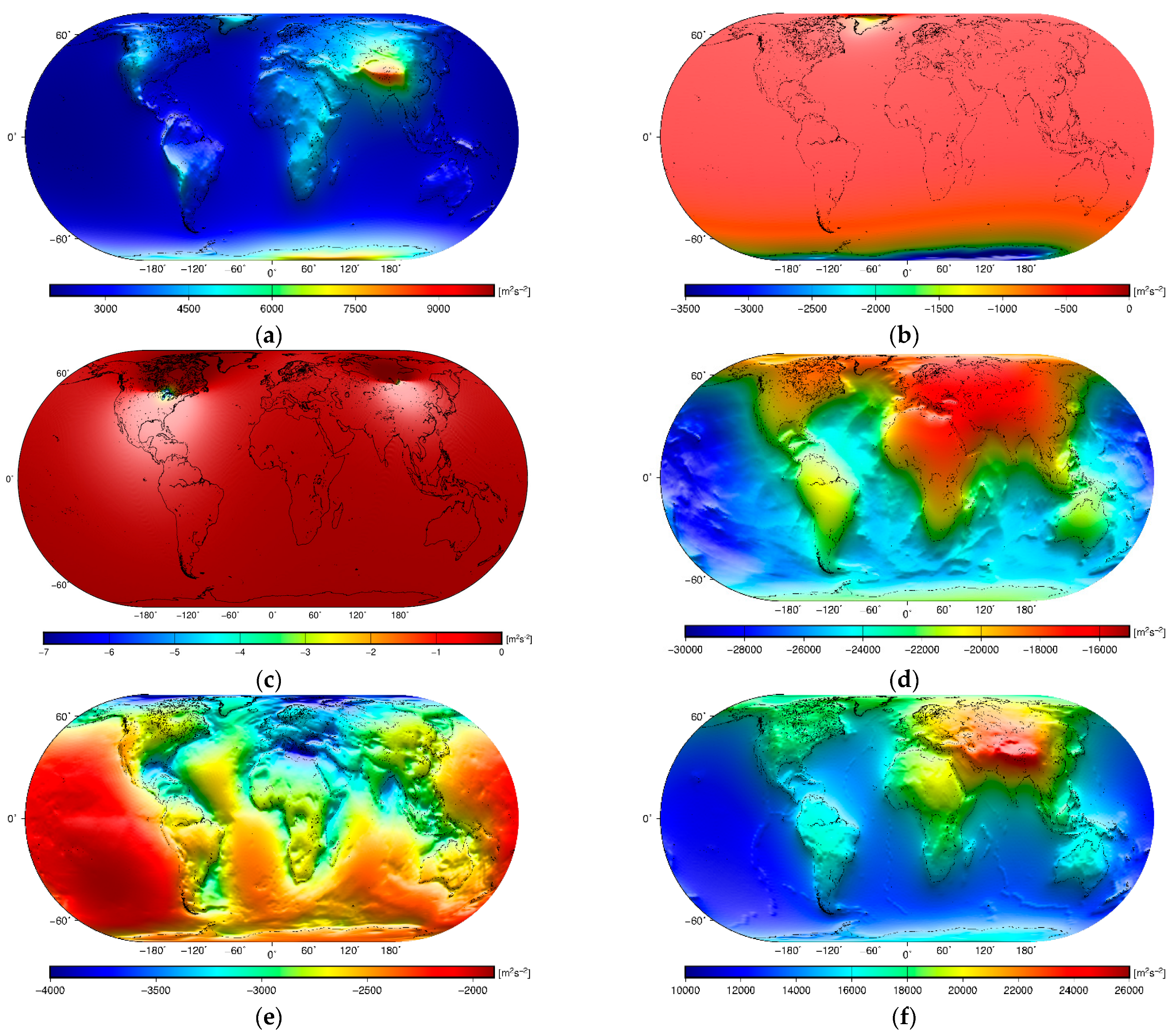
The gravitational potentials computed and applied to obtain the sub-lithospheric mantle gravity disturbances are plotted in
Figure 2, with the statistical summary of individual results given in
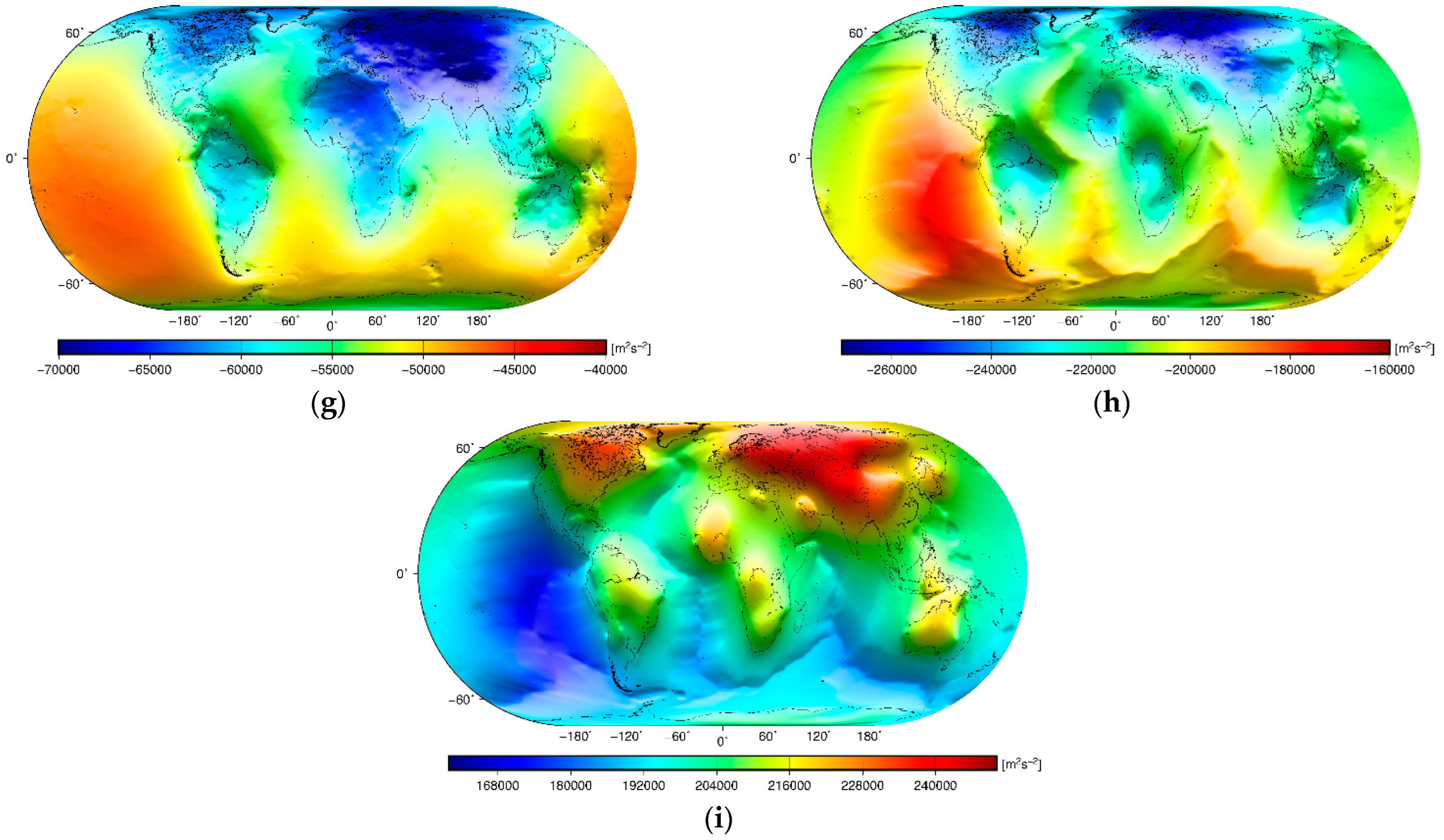
Table 1. The isostatic compensation potentials are shown in
Figure 3, with their statistics in
Table 2. The statistics of the sub-lithospheric mantle disturbing potential values and intermediate results are summarized in
Table 3. The sub-lithospheric mantle geoid together with intermediate results are presented in
Figure 4, and their statistical summary is given in
Table 4. Since the spatial patterns of disturbing potential values and corresponding geoid models are basically the same, only geoid models are visualized. In addition, the corresponding gravity maps are plotted in
Figure 5 (with statistics in
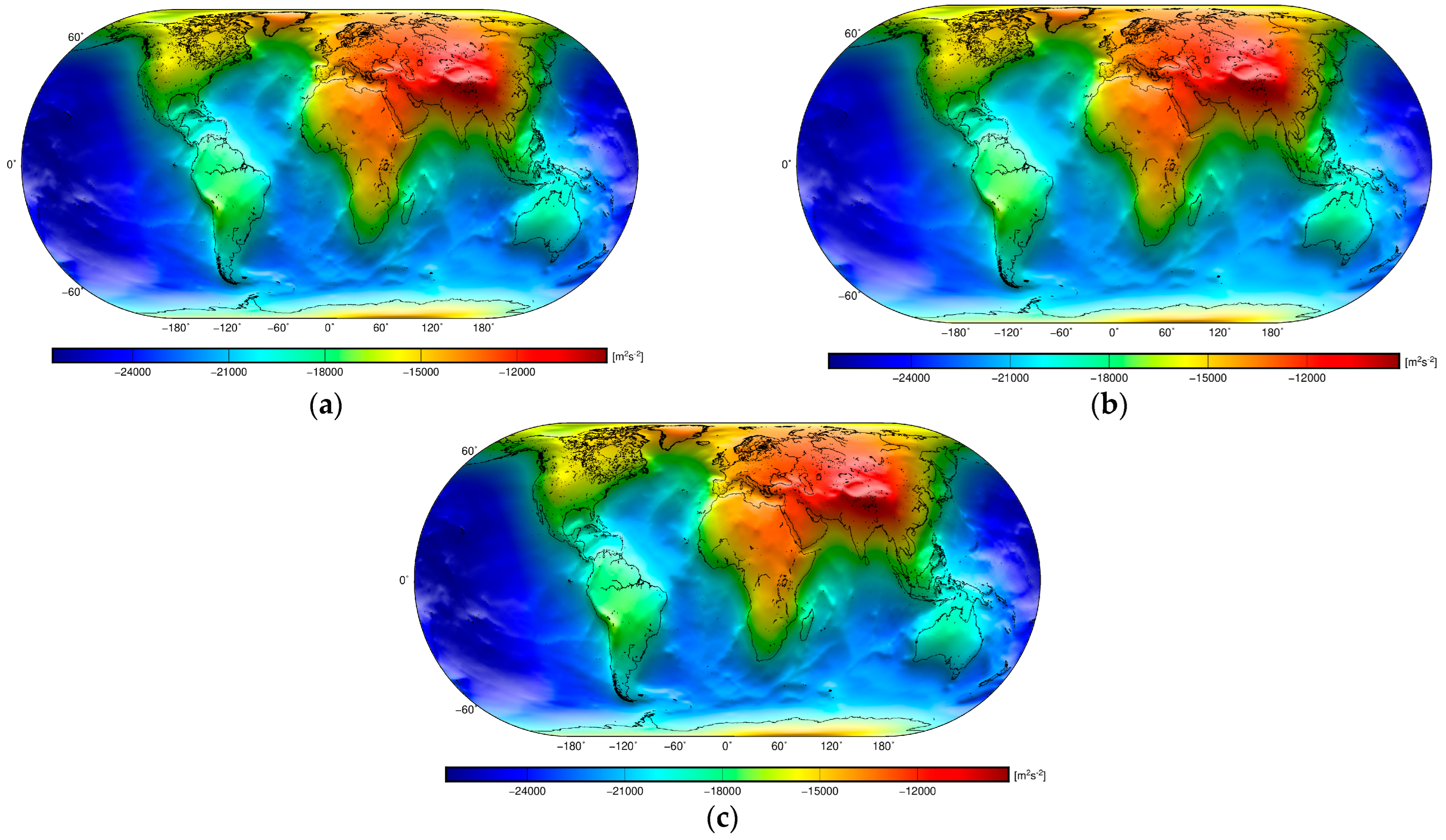
Table 5) for a comparative interpretation of geoidal and gravity maps. The isostatic geoid models are shown in
Figure 6, with the statistics given in
Table 6. For comparison, the corresponding isostatic gravity maps are also plotted in
Figure 7, and their statistics are summarized in
Table 7. The long-wavelength geoid models computed by using different degrees of the EIGEN-6C4 spherical harmonics are presented in
Figure 8, with their statistics in
Table 8.
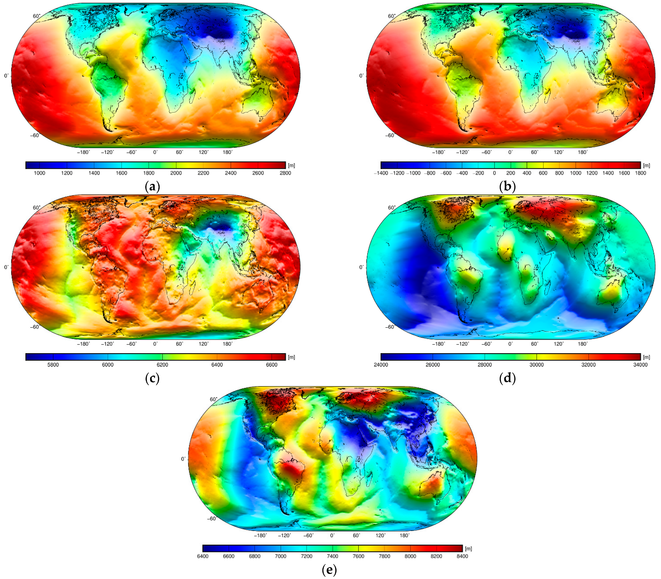
Table 1.
Statistics of the gravitational potentials of lithospheric structure. For the notation used, see the legend in
Figure 2.
Table 1.
Statistics of the gravitational potentials of lithospheric structure. For the notation used, see the legend in
Figure 2.
| Gravitational Potential | Min [m2·s−2] | Max [m2·s−2] | Mean [m2·s−2] | STD [m2·s−2] |
|---|
| 2226 | 8494 | 3589 | 1114 |
| −3472 | −312 | −731 | 729 |
| −6 | 0 | −0.2 | 0.2 |
| −28,533 | −16,402 | −22,386 | 3185 |
| −3862 | −1937 | −2719 | 444 |
| 11,529 | 25,075 | 15,661 | 2741 |
| −69,885 | −46,423 | −55,734 | 5832 |
| 174,276 | 262,661 | 213,366 | 17,795 |
| −244,558 | −168,987 | −203,311 | 16,194 |
Figure 2.
Global maps of the gravitational potentials of: (a) topography , (b) ice , (c) lakes , (d) bathymetry , (e) sediments , (f) consolidated crust , (g) Moho geometry, (h) lithospheric mantle , and (i) LAB geometry.
Figure 2.
Global maps of the gravitational potentials of: (a) topography , (b) ice , (c) lakes , (d) bathymetry , (e) sediments , (f) consolidated crust , (g) Moho geometry, (h) lithospheric mantle , and (i) LAB geometry.
Table 2.
Statistics of the isostatic compensation potentials. For the notation used, see the legend in
Figure 3.
Table 2.
Statistics of the isostatic compensation potentials. For the notation used, see the legend in
Figure 3.
| Isostatic Potential | Min [m2·s−2] | Max [m2·s−2] | Mean [m2·s−2] | STD [m2·s−2] |
|---|
| −26,859 | −9411 | −19,264 | 3905 |
| −26,347 | −9529 | −18,977 | 3791 |
| −26,860 | −9406 | −19,264 | 3910 |
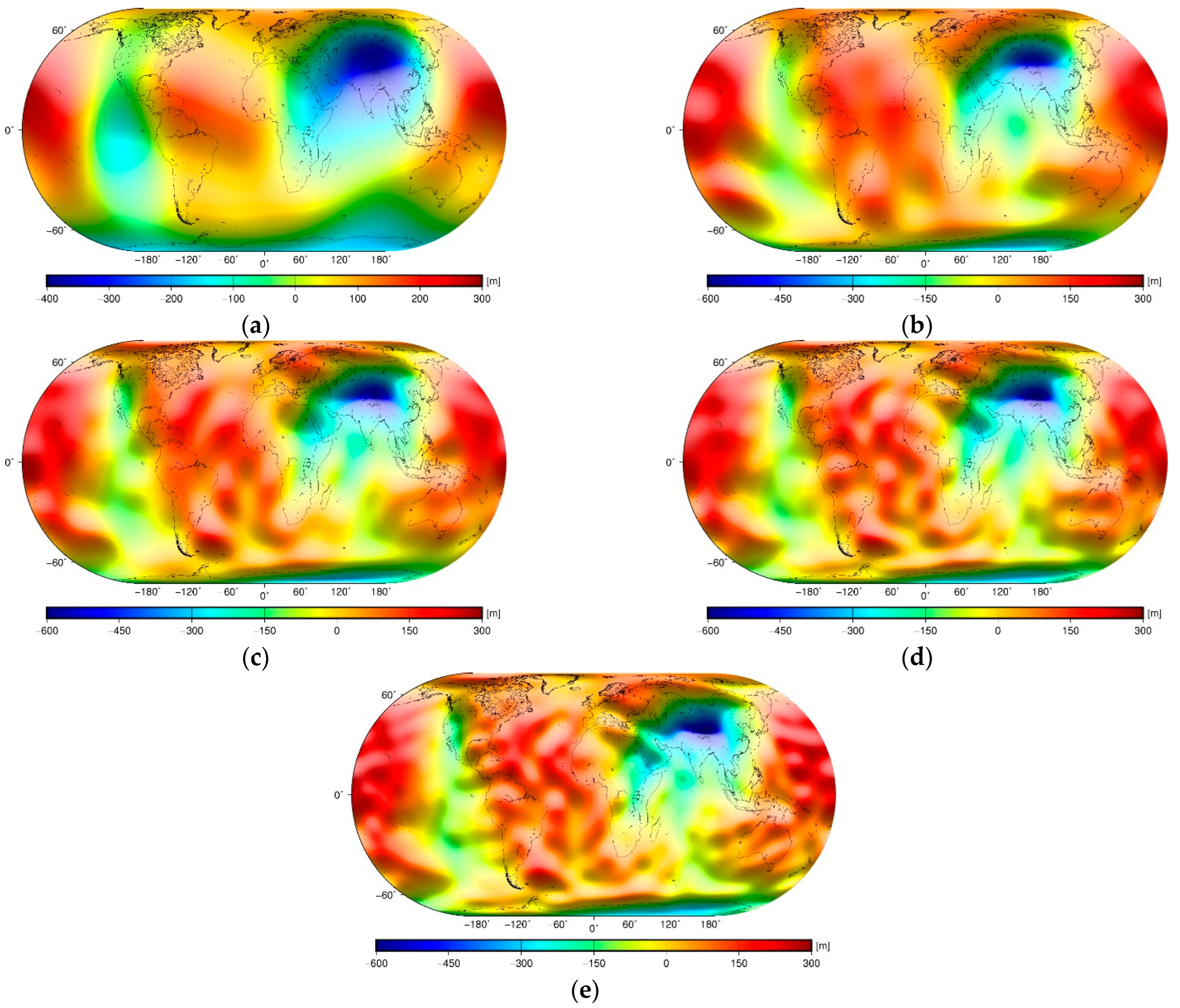
Figure 3.
Global maps of the isostatic compensation potentials: (a) Airy–Heiskanen , (b) Pratt–Hayford , and (c) Vening Meinesz–Moritz .
Figure 3.
Global maps of the isostatic compensation potentials: (a) Airy–Heiskanen , (b) Pratt–Hayford , and (c) Vening Meinesz–Moritz .
Table 3.
Statistics of the topography-corrected
, the topography- and bathymetry-corrected
, Bouguer
, crust-stripped
, mantle
, lithosphere-stripped
, and sub-lithospheric mantle
disturbing potential values. The statistics of the disturbing potential values
used to compute the geoid in
Figure 1a are also given.
| Disturbing Potential | Min [m2·s−2] | Max [m2·s−2] | Mean [m2·s−2] | STD [m2·s−2] |
|---|
| −1036 | 833 | −8 | 284 |
| −8824 | −1701 | −3595 | 1215 |
| 8589 | 26,406 | 18,793 | 3873 |
| 11,746 | 28,869 | 22,245 | 3491 |
| −13,311 | 17,086 | 6584 | 6177 |
| 56,568 | 64,854 | 62,316 | 1262 |
| 235,290 | 325,580 | 275,670 | 17,985 |
| 63,164 | 82,212 | 72,370 | 3652 |
Table 4.
Statistics of the geoid models. For the notation used, see the legend in
Figure 4.
Table 4.
Statistics of the geoid models. For the notation used, see the legend in
Figure 4.
| Refined Geoid | Min [m] | Max [m] | Mean [m] | STD [m] |
|---|
| −106 | 85 | −1 | 29 |
| 1198 | 2946 | 2269 | 356 |
| −1358 | 1743 | 671 | 630 |
| 5772 | 6617 | 6358 | 128 |
| 24,009 | 33,222 | 28,130 | 1835 |
| 6445 | 8388 | 7384 | 372 |
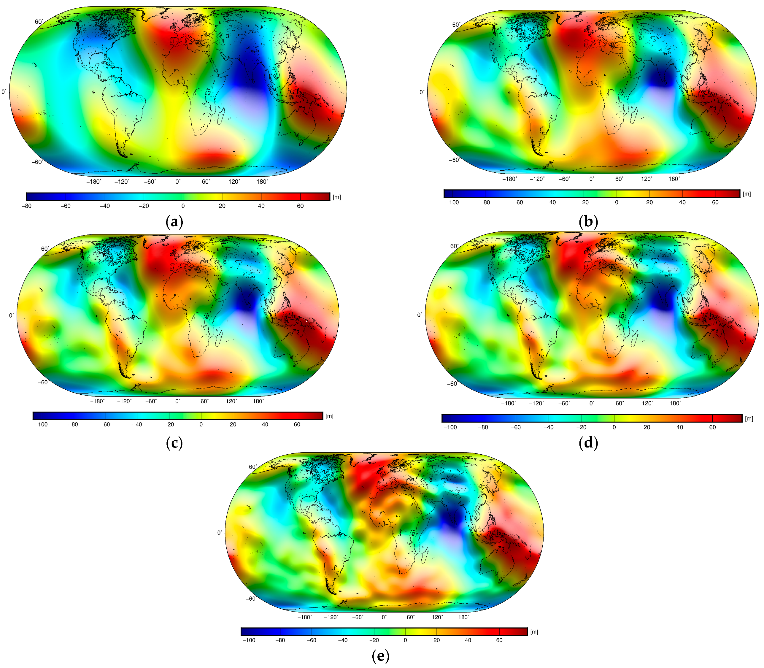
Figure 4.
Global models of: (a) the Bouguer geoid , (b) the crust-stripped geoid , (c) the mantle geoid , (d) the lithosphere-stripped geoid , and (e) the sub-lithospheric mantle geoid .
Figure 4.
Global models of: (a) the Bouguer geoid , (b) the crust-stripped geoid , (c) the mantle geoid , (d) the lithosphere-stripped geoid , and (e) the sub-lithospheric mantle geoid .
Table 5.
Statistics of the gravity disturbances. For the notation used, see the legend in
Figure 5.
Table 5.
Statistics of the gravity disturbances. For the notation used, see the legend in
Figure 5.
| Gravity Disturbances | Min [mGal] | Max [mGal] | Mean [mGal] | STD [mGal] |
|---|
| −310 | 287 | −1 | 30 |
| −492 | 743 | 329 | 225 |
| −994 | 712 | 189 | 316 |
| 393 | 1521 | 1011 | 125 |
| −7024 | −949 | −3216 | 1262 |
| 754 | 4611 | 1548 | 196 |
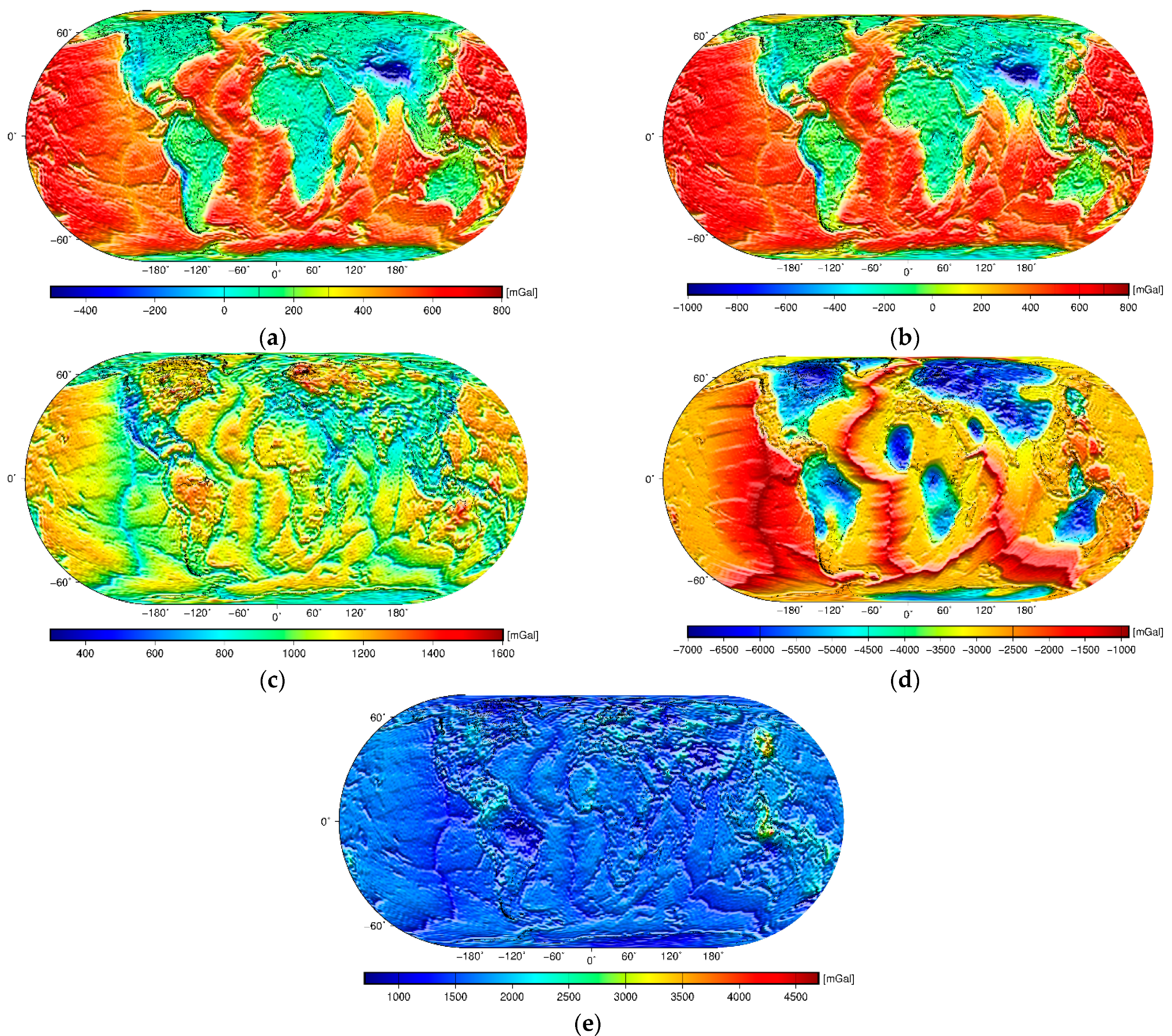
Figure 5.
Global gravity maps of: (
a) the Bouguer gravity disturbances
, (
b) the crust-stripped gravity disturbances
, (
c) the mantle gravity disturbances
, (
d) the lithosphere-stripped gravity disturbances
, and (
e) the sub-lithospheric mantle gravity disturbances
according to results presented by Tenzer and Chen [
23].
Table 6.
Statistics of the isostatic geoid models. For the notation used, see the legend in
Figure 6.
Table 6.
Statistics of the isostatic geoid models. For the notation used, see the legend in
Figure 6.
| Isostatic Geoid | Min [m] | Max [m] | Mean [m] | STD [m] |
|---|
| −108 | 74 | −8 | 30 |
| −76 | 113 | 27 | 33 |
| −108 | 75 | −8 | 30 |
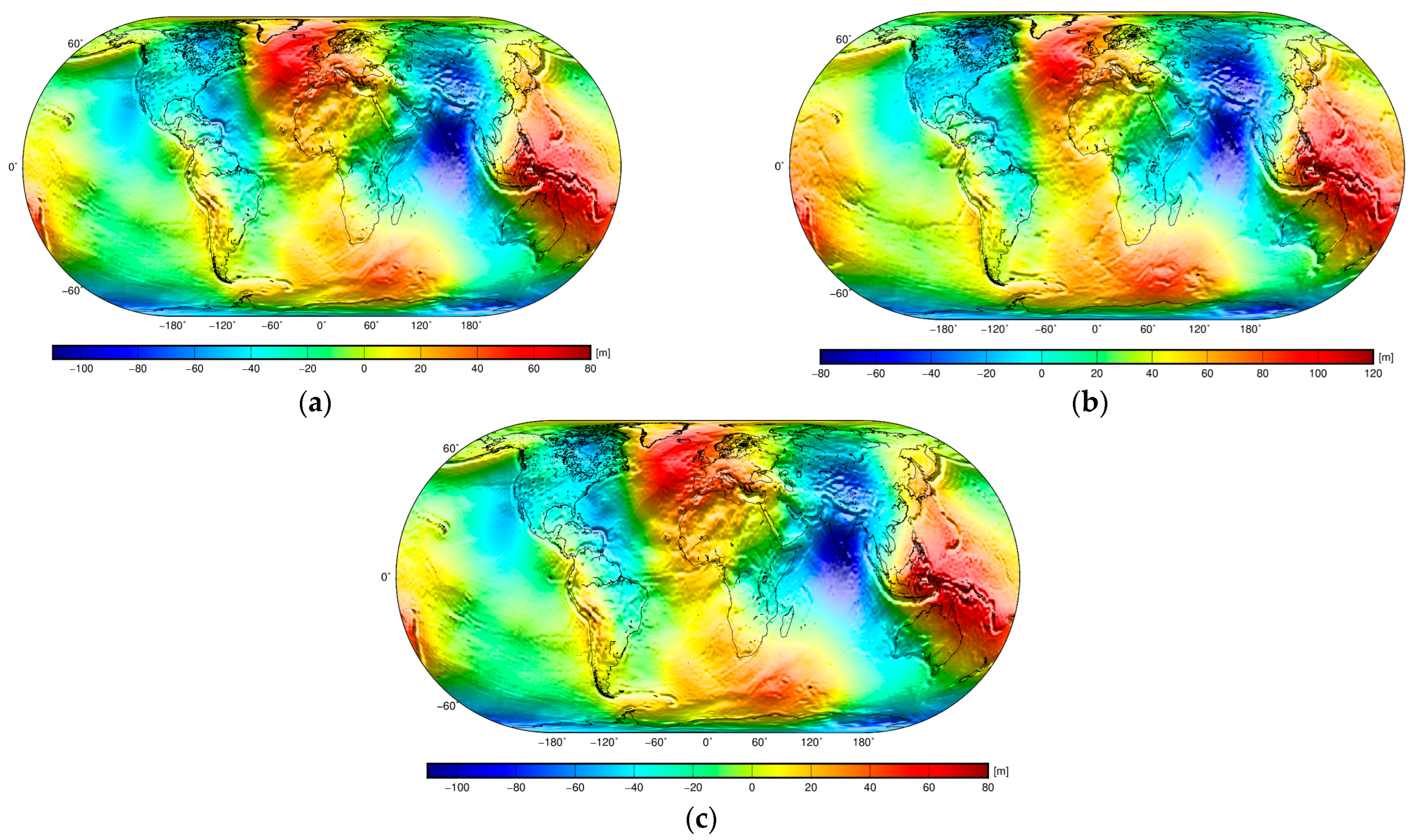
Figure 6.
Global maps of the isostatic geoid models: (a) Airy–Heiskanen , (b) Pratt–Hayford , and (c) Vening Meinesz–Moritz .
Figure 6.
Global maps of the isostatic geoid models: (a) Airy–Heiskanen , (b) Pratt–Hayford , and (c) Vening Meinesz–Moritz .
Table 7.
Statistics of the isostatic gravity disturbances. For the notation used, see the legend in
Figure 7.
Table 7.
Statistics of the isostatic gravity disturbances. For the notation used, see the legend in
Figure 7.
| Isostatic Gravity Data | Min [mGal] | Max [mGal] | Mean [mGal] | STD [mGal] |
|---|
| −267 | 227 | −2 | 28 |
| −232 | 190 | 2 | 32 |
| −260 | 221 | −2 | 28 |
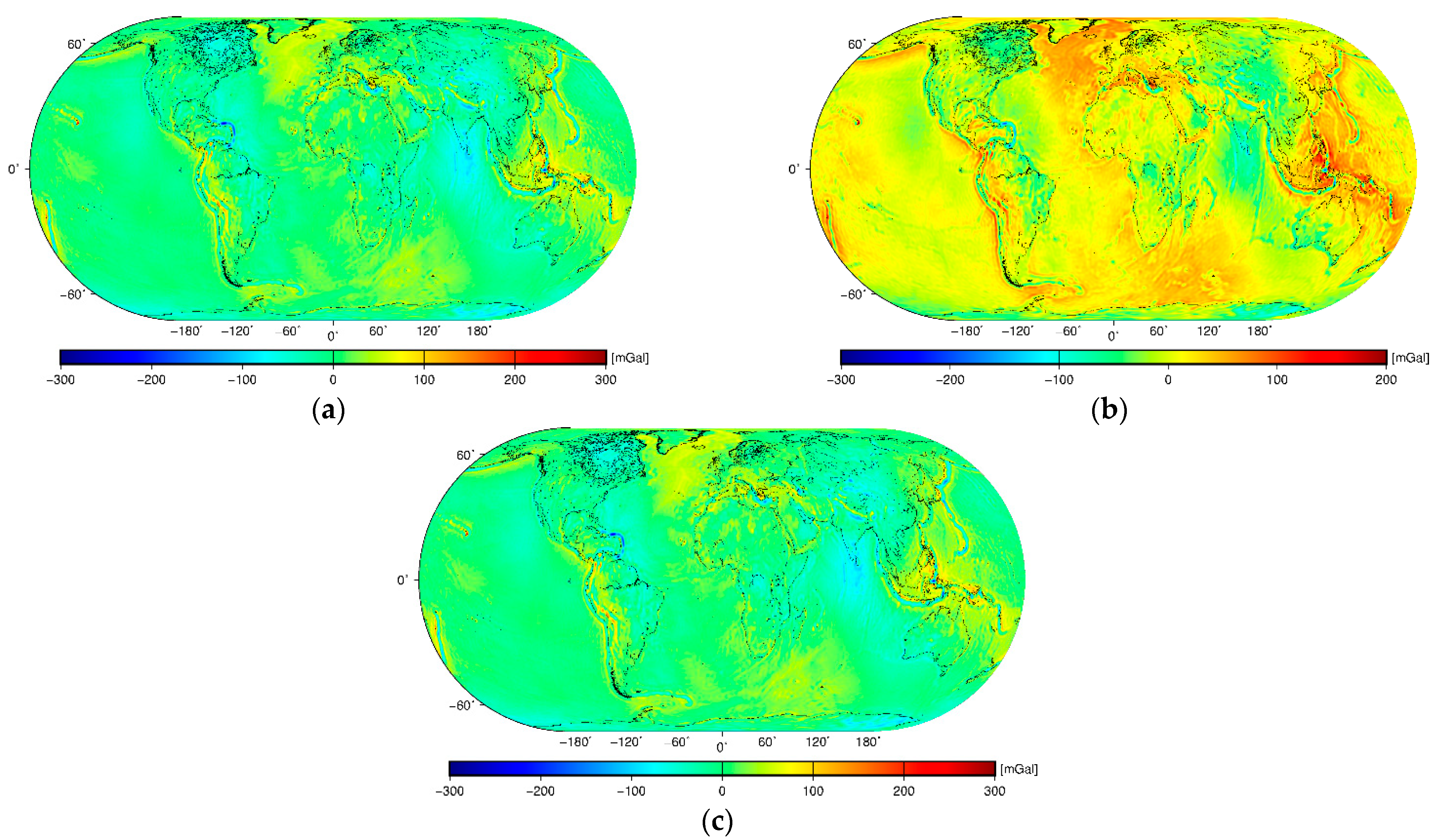
Figure 7.
Global maps of the isostatic gravity disturbances: (a) Airy–Heiskanen , (b) Pratt–Hayford , and (c) Vening Meinesz–Moritz .
Figure 7.
Global maps of the isostatic gravity disturbances: (a) Airy–Heiskanen , (b) Pratt–Hayford , and (c) Vening Meinesz–Moritz .
Table 8.
Long-wavelength geoid models computed up to a maximum degree (5, 10, 15, 20, and 25) of spherical harmonics.
Table 8.
Long-wavelength geoid models computed up to a maximum degree (5, 10, 15, 20, and 25) of spherical harmonics.
| Maximum Degree of Geoid | Min [m] | Max [m] | Mean [m] | STD [m] |
|---|
| 5 | −78 | 74 | −1 | 27 |
| 10 | −102 | 75 | −1 | 29 |
| 15 | −103 | 76 | −1 | 29 |
| 20 | −105 | 77 | −1 | 29 |
| 25 | −103 | 78 | −1 | 29 |
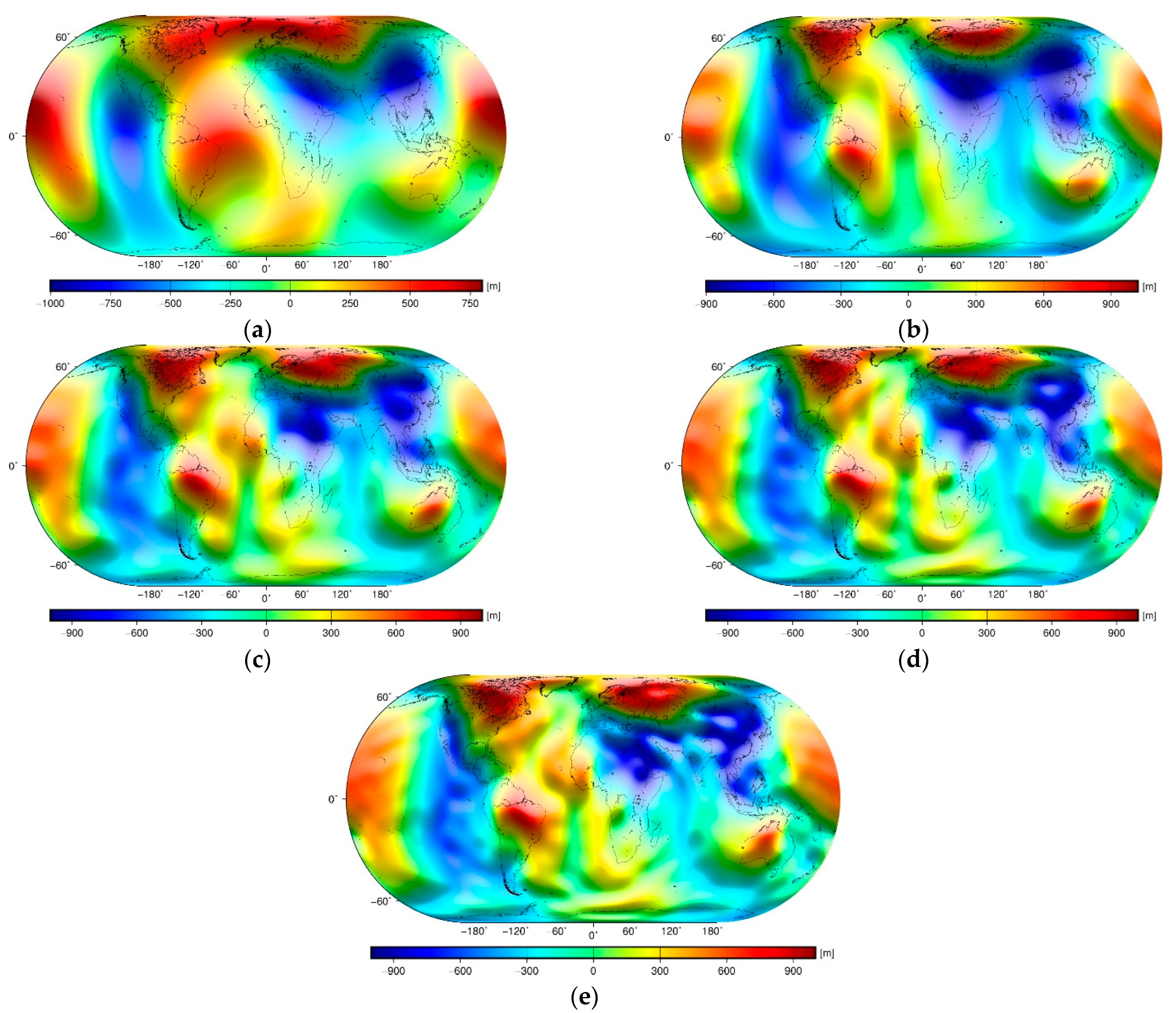
Figure 8.
Long-wavelength geoid models computed up to a maximum degree of spherical harmonics: (a) 5, (b) 10, (c) 15, (d) 20, and (e) 25.
Figure 8.
Long-wavelength geoid models computed up to a maximum degree of spherical harmonics: (a) 5, (b) 10, (c) 15, (d) 20, and (e) 25.
The global geoidal geometry (
Figure 1a) is characterized by relatively small fluctuations, mostly within ±100 m. The largest variations have a long-wavelength spatial pattern that is attributed to large-scale structures within the mantle and the crust (such as the African superswell). More localized geoidal undulations attributed mainly to topographic and ocean floor relief are, on the other hand, less pronounced. Nevertheless, we could recognize a signature of large orogens and partially also the ocean floor relief (such as some oceanic subductions, mid-oceanic ridges, and major volcanic islands). The topographic signature of the Andes is particularly well pronounced. The topographic signature of the Himalayas and Tibet is also clearly manifested, with relatively large geoidal modifications up to ~30 m along the Himalayan foothills. The spatial pattern in the free-air gravity map (
Figure 1b) is characterized by relatively small gravity fluctuations, mostly within the interval ±100 mGal. A long-wavelength pattern due to (large-scale) mantle and crustal density structures is still recognized, but this signature is much less pronounced in the gravity map than in the geoidal geometry. In contrast, the lithospheric density and geometry signature are more clearly exhibited in the free-air gravity map. Nevertheless, since most of the major topographic features and large lithospheric density structures are in an isostatic equilibrium, the largest gravity variations (roughly within ±300 mGal) mark mainly uncompensated or overcompensated structures along active convergent tectonic margins.
The most pronounced feature over continents in the Bouguer gravity map (
Figure 5a) is the isostatic signature of major orogens, while the offshore gravity pattern is dominated by a gravitational signature of the ocean floor relief. In the corresponding Bouguer geoid (
Figure 4a), this pattern is almost absent. Instead, we see a prevailing long-wavelength pattern with maxima in the Central Pacific and minima in Central Eurasia.
The crust-stripped gravity map (
Figure 5b) largely mimics a Moho geometry. The contrast between a thin oceanic crust and a much thicker continental crust is manifested by mostly positive gravity disturbances over oceans that are coupled by negative gravity disturbances over continents. The largest negative values correspond to a maximum Moho deepening under orogens of the Himalayas, Tibet, and the Andes (e.g., [
54]). A relatively vague manifestation of the isostatic signature in the Rocky Mountains was explained by their formation attributed to a flat-slab subduction of the Pacific Ocean plate underneath the North American plate (e.g., [
87]). The crust-stripped geoidal geometry (
Figure 4b) to a large extent resembles the Bouguer geoid (
Figure 4a).
The mantle gravity pattern (
Figure 5c) reflects significant lateral density variations within the lithospheric mantle that are mainly attributed to its thermal state (especially under oceans). Mantle gravity lows mark volcanically and seismically active convergent tectonic margins (in the Pacific, Mediterranean, and Caribbean). Mantle gravity lows along mid-oceanic spreading ridges increase with the ocean floor’s age. This prevailing trend was explained by an increasing density due to a conductive cooling of the oceanic lithosphere. Tenzer et al. [
55] demonstrated that the mantle gravity disturbances increase nonlinearly with the ocean floor’s age. They also identified an additional systematic trend between the mantle gravity disturbances and the ocean floor depth that was explained by thermal lithospheric contraction (due to conductive cooling) that is isostatically compensated by ocean floor deepening. For more information about the oceanic lithospheric structure and its relation with ocean floor depth and age as well as gravity changes, we refer readers to theoretical and numerical studies by Davis and Lister [
88], Sclater et al. [
89], Parsons and Sclater [
90], Parsons and McKenzie [
91], Richter and McKenzie [
92], Houseman and McKenzie [
93], Robinson and Parsons [
94], Phipps and Smith [
95], Stein and Stein [
96], Shoberg et al. [
97], DeLaughter et al. [
98], Huang and Zhong [
99], Hillier and Watts [
100], Doin and Fleitout [
101], Crosby et al. [
102], Tenzer et al. [
22], and references therein. The mantle gravity pattern over continents is more complex, reflecting the lithospheric mantle composition governed by a tectonic province configuration and its age (e.g., [
103,
104,
105,
106]). Gravity lows mark active continental divergent margins [
23], while a thermal signature along transform faults is mostly missing. Old, cold, tectonically stable cratonic formations are typically characterized by mantle gravity highs [
107].
Whereas a spatial pattern in the mantle gravity map reflects mainly the lithospheric mantle structure and its thermal state, the mantle geoidal geometry (
Figure 4c) exhibits both lithospheric mantle as well as deep mantle signatures. This is evident, for instance, in the Pacific, where we see not only the signature of a large low-shear-velocity province (LLSVP) in the Central Pacific, but also the lithospheric mantle signature of mid-oceanic ridges in the Southeast Pacific. We could recognize the thermal signature of the oceanic lithospheric mantle in the mantle geoid, even if it is much less consistent than in the corresponding mantle gravity map. The thermal signature of the continental lithospheric mantle is much less pronounced in the mantle geoidal geometry. We could partially recognize a contrast between younger orogenic lithospheric structures under the Rocky Mountains compared to the older cratonic formations of the North American Craton. Similarly, smaller mantle geoid heights along the East African Rift System and along the Red Sea Rift are coupled by larger values over cratonic formations that form most of West Africa. Moreover, mantle geoid lows along the Alpine-Himalayan orogenic belt are coupled to the north by larger values over cratonic formations in North Eurasia. These findings indicate that the thermal signature of the lithospheric mantle is still more or less superimposed over the mantle convection signature in the mantle geoid pattern.
The lithospheric thickness variations are the most pronounced features in the lithosphere-stripped gravity (
Figure 5d) and geoid (
Figure 4d) maps. Similarities in both spatial patterns are explained by the relatively deep location of the LAB. Nevertheless, the LAB geometry is obviously still slightly more pronounced in the lithosphere-stripped gravity map. As stated above, the lithosphere-stripped gravity and geoid maps exhibit a very similar spatial pattern attributed to the lithosphere–asthenosphere boundary. Contrary to this finding, the spatial patterns in the sub-lithospheric mantle gravity (
Figure 5e) and geoid (
Figure 4e) maps completely differ. In the former, gravity lows to some extent mark mantle upwelling currents under mid-oceanic spreading ridges. Tenzer and Chen [
23] explained this finding by the existence of a molten asthenosphere, particularly below mid-oceanic spreading ridges, although the asthenosphere is mostly almost solid. Nonetheless, the sub-lithospheric mantle gravity map in fact does not exhibit any particular density structure anomaly, except for a more pronounced signature of subducted slabs in the West Pacific. The thermal signature of the asthenosphere under the continental lithospheric mantle is slightly more pronounced under some cratonic formations (Laurentian, Baltic and Amazonian Shields, and São Francisco and East Antarctic Cratons). This finding agrees with the hypothesis that in the thickest cratonic portions of very fast seismic velocity (e.g., [
108,
109]), the cold and dense layers within the cratonic crust or the lithospheric mantle are isostatically compensated and neutrally buoyant due to the positive buoyancy of depleted cratonic mantle peridotites [
110].
The sub-lithospheric mantle geoid pattern (
Figure 4e) differs significantly from the long-wavelength geoidal geometry (
Figure 1a). The West Pacific geoid high is mostly absent, while the sub-lithospheric mantle geoid high spreads over most of the Central Pacific. The North Atlantic geoid high is also absent in the sub-lithospheric mantle geoid map. Instead, we see two geoid highs in the Hudson Bay region and Northeast Eurasia. The Indian Ocean geoid low coincides with the sub-lithospheric mantle geoid low, but this anomaly is distributed much more broadly over most of South Eurasia while further spreading over Northeast Africa and the North Indian Ocean. The sub-lithospheric mantle geoid high in the Central Pacific is apparently delineated by oceanic subductions in the North Pacific and by mid-oceanic ridges in the East Pacific, but the exact location of their margins could not clearly be ascertained (due to a prevailing long-wavelength geoidal pattern). A more detailed discussion of these findings is postponed until
Section 5.
The Airy–Heiskanen, Pratt–Hayford, and Vening Meinesz–Moritz isostatic geoids (
Figure 6) very closely resemble the long-wavelength geoidal geometry (
Figure 1a). Interestingly, even more detailed features in all three isostatic geoid models are very similar to the geoid pattern. We could still depict, for instance, the topographic signature of Tibet and the Himalayas, especially along the Himalayan foothills, even after applying isostatic correction. The largest localized differences between the geoid and isostatic geoids are seen along the Andes, where the topographic signature is almost completely removed. The Airy–Heiskanen and Vening Meinesz–Moritz isostatic gravity maps (
Figure 7a,c) are very similar, with both having a smooth pattern. The application of isostatic correction thus removed the signature of isostatically uncompensated or overcompensated lithospheric structures to a large extent, especially along active convergent tectonic margins. As a result, the long-wavelength pattern is more pronounced in both isostatic geoid models. Interestingly, this long-wavelength pattern is more clearly manifested in the Pratt–Hayford isostatic geoid (
Figure 7b).
As seen in
Figure 8, the spatial decomposition gradually filters out more detailed features in the geoidal geometry when decreasing the maximum degree of spherical harmonics used to compute the geoid models. Nevertheless, the topographic signature of Tibet and the Himalayas is still partially displayed in the long-wavelength geoidal geometry computed up to a degree of 10 and higher. This topographic signature becomes almost completely absent only in the geoidal geometry computed up to a maximum degree of 5. These results confirm that the separation of gravitational signatures from different depth structures inside the Earth is not unique. Thus, this method works only under the assumption that anomalous density structures increase with depth. In reality, however, this trend is typically the opposite (i.e., the largest density variations are within the upper crust).
6. Summary and Concluding Remarks
We investigated the possibility of enhancing a mantle signature in the long-wavelength geoidal geometry by applying gravimetric, isostatic, and spectral decomposition methods. In the gravimetric method, we applied gravimetric forward modelling to isolate and subsequently remove the gravitational contributions of crustal density and geometry variations from the geoidal geometry in order to enhance the mantle signature. In the isostatic method, we applied the Airy–Heiskanen, Pratt–Hayford, and Vening Meinesz–Moritz isostatic compensation schemes for this purpose. In the spectral decomposition method, we computed the long-wavelength geoidal geometry with a limited spectral resolution. In addition, we also inspected the possibility of using a filtering technique, but our results (not presented in this study) showed that the Gauss filter did not sufficiently smooth the geoidal geometry.
According to our numerical results, the gravimetric forward modelling better enhanced the mantle signature in the geoidal geometry than the isostatic and spectral decomposition methods. Whereas the former modified the geoidal geometry substantially, the latter mostly only smoothed the long-wavelength geoidal geometry. A similar finding was related to mantle and isostatic gravity maps. Whereas the mantle gravity map relatively realistically manifested a thermal signature of the lithospheric mantle, the isostatic gravity maps mostly enhanced the long-wavelength gravity pattern that very closely agreed with the corresponding long-wavelength geoidal geometry. Evidently, the concerning question is how realistic modifications of the geoidal geometry by subtracting the gravitational contribution of crust are, because available global models of the crustal density structure and geometry (such as the CRUST1.0 and LITHO1.0 models) have a limited accuracy and resolution.
We further used lithospheric models to subtract the gravitational contributions of lithospheric mantle density and lithospheric thickness variations from the mantle geoid. This procedure yielded the sub-lithospheric mantle geoid that should better exhibit the signature of the mantle convection pattern than the mantle geoid. The result revealed the existence of two positive sub-lithospheric mantle geoid anomalies in the Central Pacific and along the Atlantic Ocean and two negative anomalies in the East Pacific and South Eurasia.
Despite the overall similarities between the major features in the sub-lithospheric mantle geoid and dynamic topography models, large differences between their spatial patterns were also found. This finding confirmed that the spatial pattern of the sub-lithospheric mantle geoid is not compatible (despite overall similarities) with the spatial pattern of dynamic topography. The main reason is that the former reflects lateral mantle density anomalies below the lithosphere–asthenosphere boundary, while the latter represents topographic manifestations of vertical stresses due to convection flow. Moreover, large positive anomalies in the sub-lithospheric mantle geoid at locations with a maximum lithospheric thickness suggest large inaccuracies in the CRUST1.0 and LITHO1.0 models. A detailed inspection of these errors will be the subject of a forthcoming study.


