Article

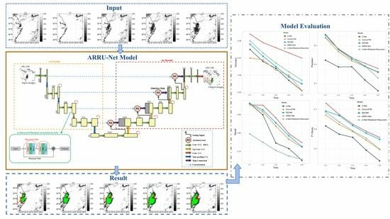
Recognition of Severe Convective Cloud Based on the Cloud Image Prediction Sequence from FY-4A

1
Faculty of Information Science and Engineering, College of Marine Technology, Ocean University of China, Qingdao 266100, China
2
Laoshan Laboratory, Qingdao 266237, China
3
Sanya Oceanographic Institution, Ocean University of China, Sanya 572024, China
4
PLA Unit 31016, Beijing 100081, China
5
Key Laboratory of Science and Technology on Operational Oceanography, Chinese Academy of Sciences, Guangzhou 510301, China
*
Author to whom correspondence should be addressed.
Remote Sens. 2023, 15(18), 4612; https://doi.org/10.3390/rs15184612
Submission received: 8 August 2023 / Revised: 15 September 2023 / Accepted: 18 September 2023 / Published: 20 September 2023
(This article belongs to the Special Issue Analysis of Satellite Cloud Images via Deep Learning Techniques)

Abstract

:
Severe convective weather is hugely destructive, causing significant loss of life and social and economic infrastructure. Based on the U-Net network with the attention mechanism, the recurrent convolution, and the residual module, a new model is proposed named ARRU-Net (Attention Recurrent Residual U-Net) for the recognition of severe convective clouds using the cloud image prediction sequence from FY-4A data. The characteristic parameters used to recognize severe convective clouds in this study were brightness temperature values TBB9, brightness temperature difference values TBB9−TBB12 and TBB12−TBB13, and texture features based on spectral characteristics. This method first input five satellite cloud images with a time interval of 30 min into the ARRU-Net model and predicted five satellite cloud images for the next 2.5 h. Then, severe convective clouds were segmented based on the predicted image sequence. The root mean square error (RMSE), peak signal-to-noise ratio (PSNR), and correlation coefficient (R2) of the predicted results were 5.48 K, 35.52 dB, and 0.92, respectively. The results of the experiments showed that the average recognition accuracy and recall of the ARRU-Net model in the next five moments on the test set were 97.62% and 83.34%, respectively.

Graphical Abstract

1. Introduction

Cloud research is paramount in atmospheric and meteorological systems. The recognition of severe convective clouds has always been important in researching meteorological disaster prevention [1,2,3].
The task of satellite cloud image prediction is a time-space sequence prediction task, which is to predict the position and shape of the cloud cluster and the change of brightness temperature value of the infrared channel for a certain period. Currently, there are three methods to predict satellite cloud images: block matching, optical flow, and artificial intelligence. Jamaly et al. improved the accuracy of cloud motion estimation regarding velocity and direction by utilizing the cross-correlation and cross-spectrum analysis methods as matching criteria based on the block matching principle [4]. Dissawa et al. proposed a method for real-time motion tracking of clouds based on cross-correlation and optical flow and applied it to the entire sky image based on the ground [5]. Shakya et al. developed a fractional-order technique for calculating optical flow and applied it to cloud motion estimation in satellite image sequences. In addition, cloud prediction was carried out using optical flow interpolation and extrapolation models based on conventional anisotropic diffusion [6]. In recent years, under the background of big data, more and more artificial intelligence methods have been used to predict cloud images. Son et al. proposed a deep learning model (LSTM–GAN) based on cloud movement prediction in satellite images for PV forecasting [7]. Xu et al. proposed a generative antagonistic network-long-short memory model (GAN-LSTM) for FY-2E satellite cloud image prediction [8]. Bo et al. used a convolutional short-term memory network to predict cloud position. This method can realize end-to-end prediction without considering the speed and direction of cloud movement [9]. Traditional methods and existing artificial intelligence methods have problems with low-resolution and blurred images in cloud image extrapolation.
One of the main bases for recognizing severe convective clouds using satellite imagery is spectral signatures. Many scholars have proposed several brightness temperature thresholds for the identification of severe convective clouds in different research areas, such as 207 K [10], 215 K [11], 235 K [12], etc. Mecikalski et al. used infrared water vapor brightness temperature difference and bright temperature difference between split widow channels as one of the criteria for recognizing severe convective clouds [13]. Jirak et al. have studied hundreds of mesoscale convective systems for four months continuously and aimed to identify convective clouds in infrared cloud images by using the brightness temperature value of a black body of less than 245 K as the recognition condition [14]. Sun et al. reduced false detection by introducing the different information of two channels and improving the effect of the algorithm in penetrating recognition of convective clouds [15]. Mitra et al. created a multi-threshold approach to detect severe convective clouds throughout the day and at night [16].
In addition to spectral characteristics, cloud texture structure can be used as an essential basis for recognition. Welch et al. used a gray-level co-occurrence matrix to extract LANDSAT satellite images for cloud classification and achieved good results [17]. Zinner combined the displacement vector field calculated according to the image-matching algorithm and the spectral images of adjacent times to determine the regions with severe convective development in the cloud map, and the images of different bands were used to recognize severe convective clouds at different stages of development [18]. Bedka et al. proposed an infrared window zone texture method to identify the upward thrust of severe convective clouds [19].
This study has improved the ability of the disaster warning system to predict severe convective weather, providing more accurate guidance in mitigating the impact of severe convective weather-induced disasters. First, to improve the accuracy of recognizing severe convective clouds, we proposed using the ARRU-Net network for predicting the following 2.5 h of satellite cloud images and recognizing convective clouds within them. Second, we introduced the attention mechanism, the residual model, and the recurrent convolution to enhance the prediction and recognition capabilities of the model. Third, we integrated severe convective clouds’ spectral and texture features to explore more feature parameters and improve recognition accuracy. This method eliminated cirrus clouds and increased the recognition accuracy of severe convective clouds.
The rest of the paper is organized as follows. The study area, the FY-4A satellite AGRI Imager data, and data processing are described in Section 2. The configuration of the ARRU-Net model, severe convective cloud label-making method and model performance evaluation method are described in Section 3. The comparison experiments of cloud image prediction and recognition of severe convective cloud based on the cloud image prediction sequence are described in Section 4. The conclusions are given in Section 5.

2. Study Area and Data
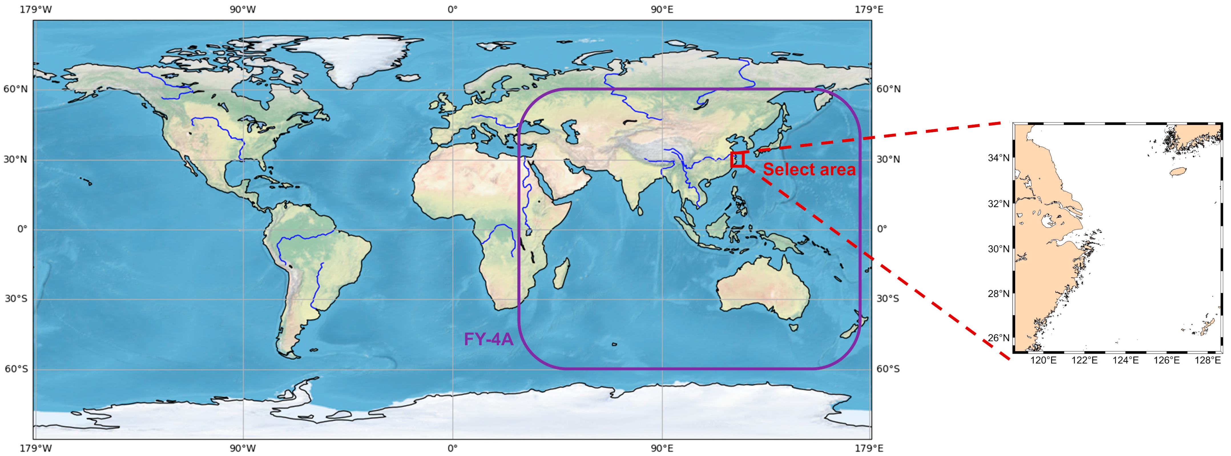
2.1. Study Area

The study area was latitude of 118.52°E–128.72°E and longitude of 25.28°N–35.48°N, covering the eastern coast of China and the northwest Pacific. The study area is shown in Figure 1. Because the eastern part of China is connected with the western part of the Pacific Ocean, the change of cloud systems there is more active. Introducing the information of cloud systems in the western part of the Pacific Ocean into the study area has a good auxiliary effect on the cloud system prediction in the coastal areas of China.

2.2. FY-4A Data

There are several meteorological detection sensors onboard FY-4A. Among them, AGRI Imager can scan an area in minutes, adopt the off-axis three-mirror main optical system, obtain more than 14 bands of earth cloud images at high frequency, and use an onboard black body for high-frequency infrared calibration to ensure the accuracy of observation data. AGRI consists of a total of 14 channels that span the range from visible to infrared light. These channels cover a wide geographical area, ranging from 80.6°N to 80.6°S and from 24.1°E to 174.7°W [20]. Since the visible light and shortwave infrared band of the FY-4A satellite cannot be used at night, this paper selected water vapor and long-wave infrared channel data from the L1 data of the multi-channel imager of FY-4A satellite for all-weather cloud prediction and strong convective cloud identification. Figure 2 shows an example of cloud data from 14 channels of the FY-4A satellite AGRI Imager. The observational parameters for each channel are presented in Table 1.

2.3. Data Preprocessing

Before using FY-4A AGRI Imager data for the study, it was necessary to preprocess the data, which mainly included geometric correction, radiometric calibration, and data normalization. After radiation calibration, the grayscale images were converted into brightness temperature images. The original raster files were projected onto a unified coordinate system through geometric correction. The data were then normalized to eliminate the influence caused by differences in the value range.

2.3.1. Geometric Correction

In the L1 data of the FY-4A AGRI Imager, a corresponding calibration table is provided for the image data layer of each channel. If we take the DN value corresponding to a particular position in the image data layer as an index, we then find the reflectivity or brightness temperature value corresponding to the index position in the calibration table to realize the radiation calibration process. Before using FY-4A AGRI Imager data for the study, it was necessary to preprocess the data, which mainly included data extraction, geometric correction, radiometric calibration, and data normalization.

2.3.2. Radiometric Calibration

The latitude and longitude data selected in this paper range from 118.52°E to 128.72°E and 25.28°N to 35.48°N. The formula for calculating the number of rows in the projected image is as follows,
c o l u m n = l o n m a x l o n m i n r e s
r o w = l a t m a x l a t m i n r e s
where c o l u m n denotes the number of columns of the image after projection, and r o w represents the number of rows after projection. l o n m a x , l o n m i n denote the maximum and minimum values of the longitude range, l a t m a x , l a t m i n denote the maximum and minimum values of the latitude range, and r e s represents the spatial resolution of the data used in this study, which was 0.4°.
Each pixel in the original satellite image was mapped into the projected image by the equal longitude and latitude projection transformation formula, which is as follows,
x = l o n l o n m i n r e s
y = l a t m a x l a t r e s
where x represents the abscissa in the image after projection, and y represents the ordinate in the image after projection.

2.3.3. Data Normalization

The data used in this study were the FY-4A satellite multi-channel imager water vapor and long-wave infrared band (FY-4A AGRI Imager 9–14 channel) data, and these bands after radiation calibration processing. The value in the channel was brightness temperature value, and the data range of the brightness temperature values was determined to be 124~325 by calibration. Therefore, for mapping purposes, this paper assigned 124 as the minimum value and 325 as the maximum value and mapped the data to the [0, 1] interval through the calculation method of the following formula,
x * = ( x m i n ) ( m a x m i n )  
where m i n is the minimum value in the sample data and m a x is the maximum value of the sample data.

3. Method

Based on the U-Net network [21] with the attention mechanism, the recurrent convolution, and the residual module, a new model was proposed, named ARRU-Net, for the recognition of severe convective clouds using the cloud image prediction sequence from FY-4A data. The data used in this study were the FY-4A AGRI imager 9–14 channel data. This method first input five satellite cloud images with a time interval of 30 min into the ARRU-Net model and predicted five satellite cloud images for the next 2.5 h. Then, the ARRU-Net model segmented the severe convective clouds based on the predicted image sequence.

3.1. The Proposed ARRU-Net Model

Based on the U-Net network, this study introduces a new network named ARRU-Net using the attention mechanism and the residual module, which changes the original U-Net convolution into a recurrent convolution, as shown in Figure 3.

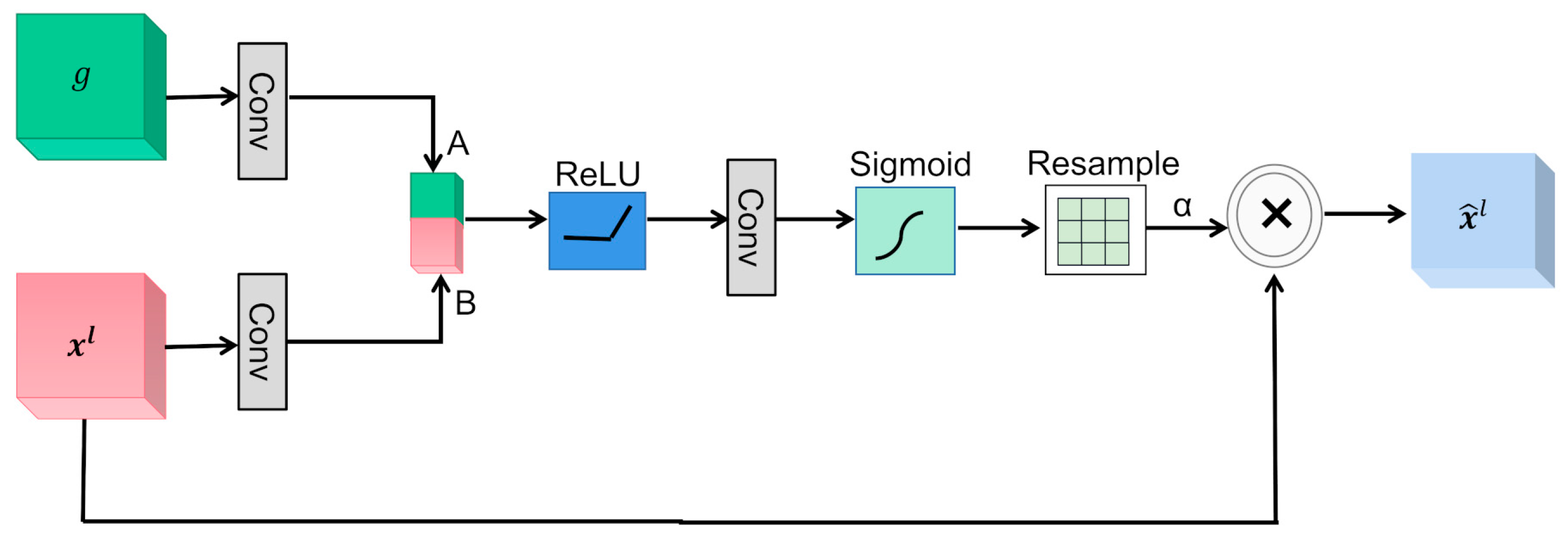
3.1.1. Attention Mechanism

In meteorological satellite data, surrounding geographical features and the resemblance between snow cover and cloud clusters can cause the learning direction of models to deviate from the intended target. Additionally, meteorological satellite data contain multiple spectral channels, each playing a distinct role in cloud detection. In light of these challenges, incorporating an attention mechanism into cloud detection models for meteorological satellite imagery can facilitate the focused learning of differences between cloud clusters and other regions and the varying impacts of each channel on cloud formation. This approach aims to enhance the efficiency and accuracy of cloud detection.
The structure of the attention module is shown in Figure 4. This attention mechanism takes two feature maps as inputs, g and xl, which are linearly transformed into A and B through 1 × 1 convolution. The resulting feature maps are then added together and passed through a ReLU activation function to obtain the intermediate feature map. After another 1 × 1 convolution operation, as well as sigmoid function and resampling, the attention coefficient α is obtained. Finally, the attention coefficient α is multiplied by xl to obtain the output feature map.

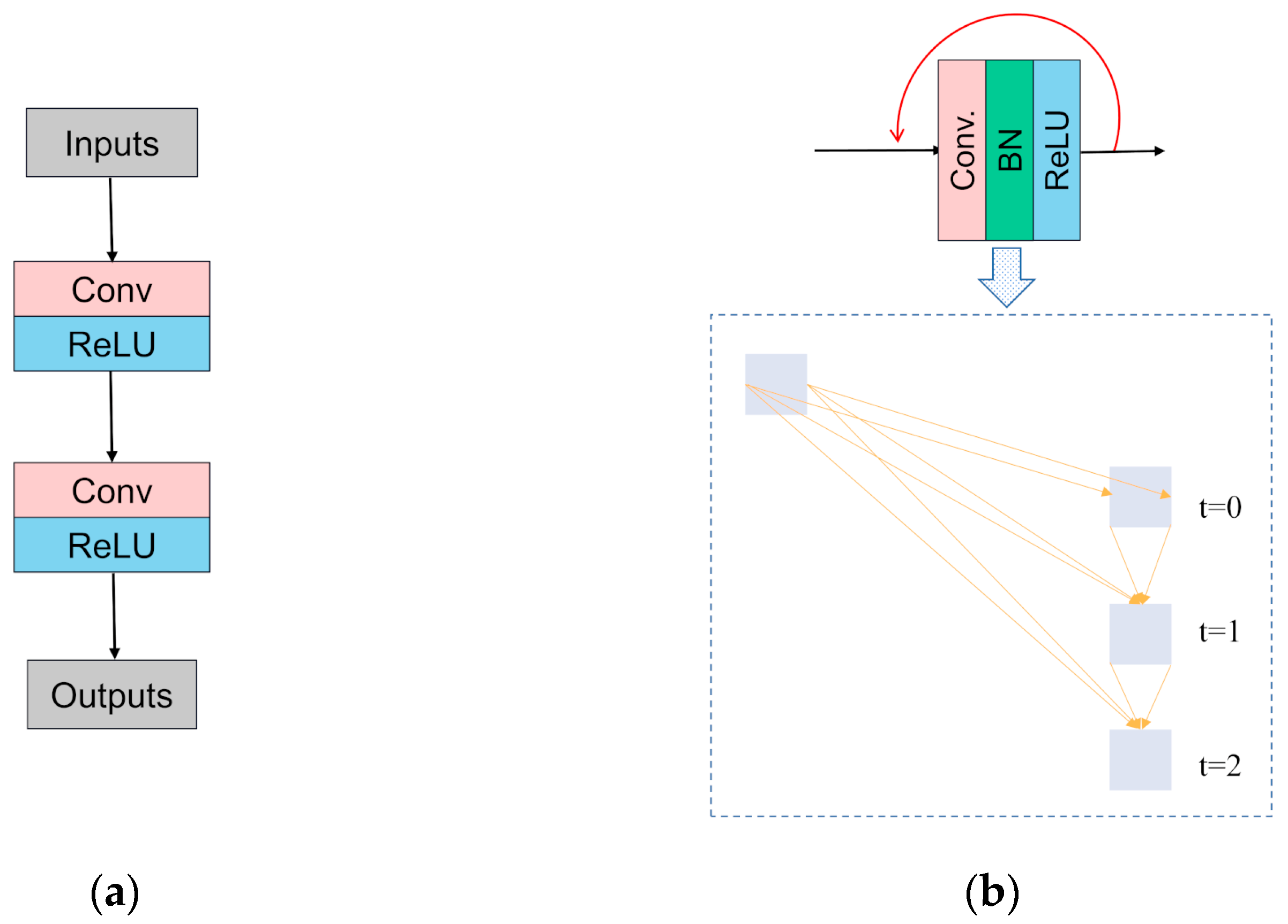
3.1.2. Recurrent Convolutional Block

Recurrent convolution is widely employed in text classification [22]. It has also found applications in computer vision, such as object recognition, as demonstrated by Liang et al. [23], and image segmentation, as demonstrated by Alom et al. [24].
This model changes the convolutional layers of U-Net into recurrent convolutional layers to learn multi-scale features of different receptive fields and fully utilize the output feature map, as shown in Figure 5. Recurrent convolution can extract spatial features from cloud imagery data by applying convolutional operations at each time step. These features capture information such as different cloud types’ shapes, textures, and structures, thereby providing richer input features for subsequent predictive tasks. In each recurrent convolutional block, the Conv + BN + ReLU operation is repeated t times by adjusting the total time step parameter to t.

3.1.3. Residual Connection

Residual connection [25] is a widely used technique in deep learning. Using direct summation, it combines the final output with a nonlinear transformation of the original output and the input. This method has been shown to effectively address issues such as network degradation [26,27] and shattering gradient during backpropagation, while also making training easier.
The residual connection enables the direct addition of the input cloud imagery to the output cloud imagery, thereby supplementing the lost feature information during the convolutional process. It also helps mitigate the degradation problem often observed in deep networks, allowing for extracting more comprehensive cloud characteristics within convolutional layers of the exact resolution. Consequently, this approach enhances the model’s generalization capability. The structure of the residual connection is shown in Figure 6.

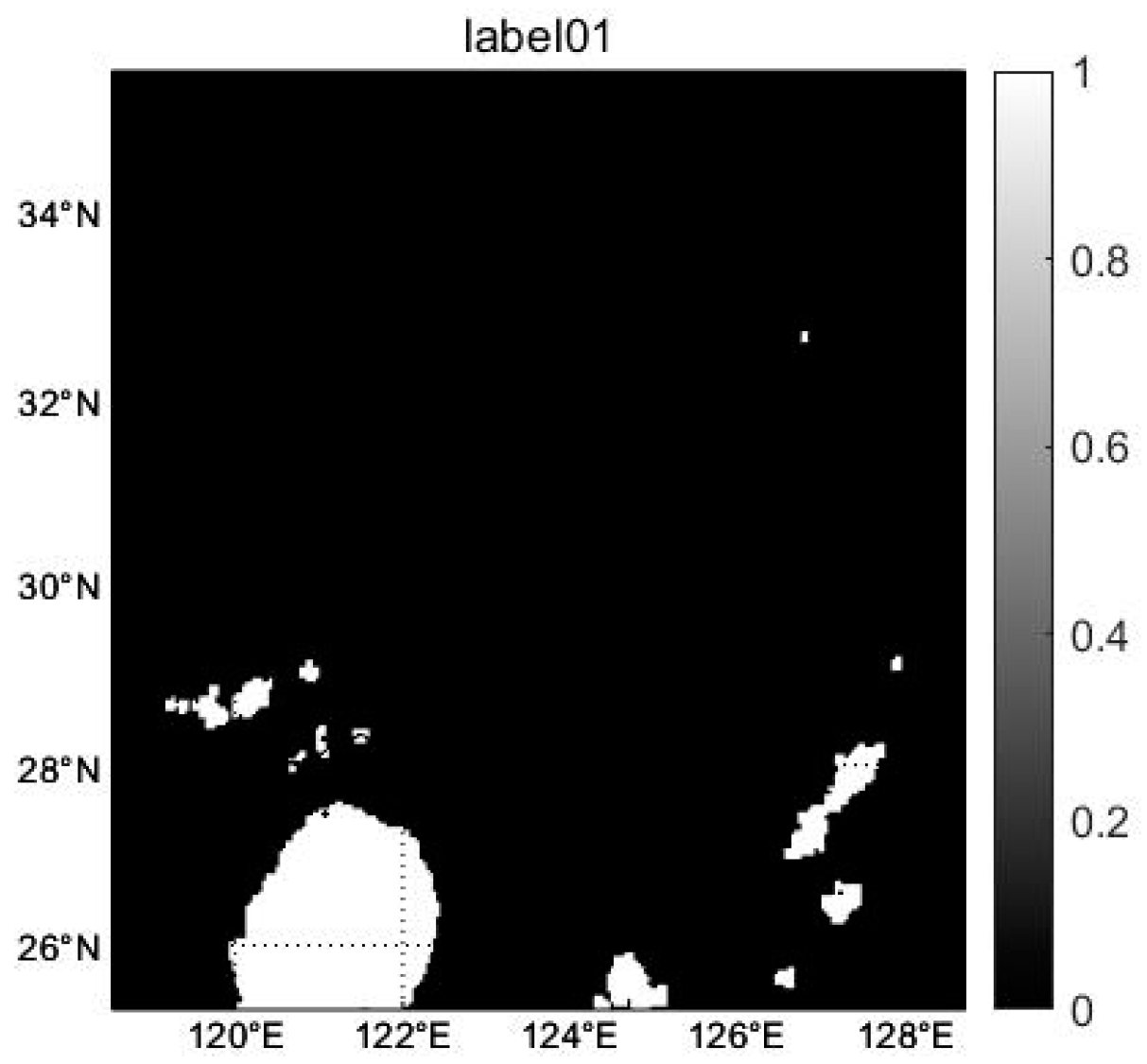
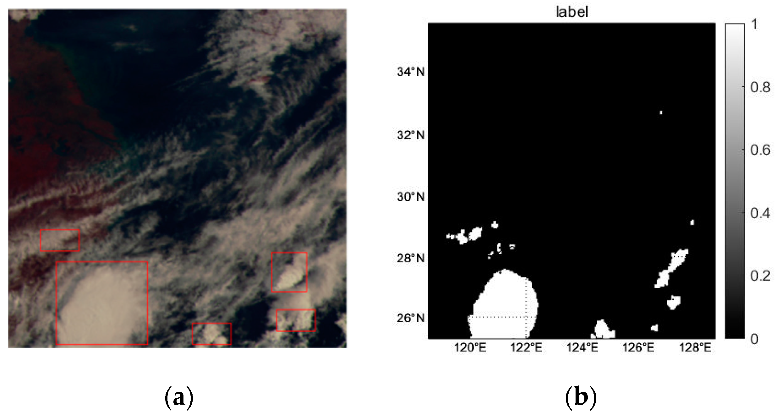
3.2. Severe Convective Cloud Label-Making Method

The characteristic parameters used to recognize severe convective clouds in this study were brightness temperature value TBB9, brightness temperature difference values TBB9−TBB12 and TBB12−TBB13, and texture features based on spectral characteristics.

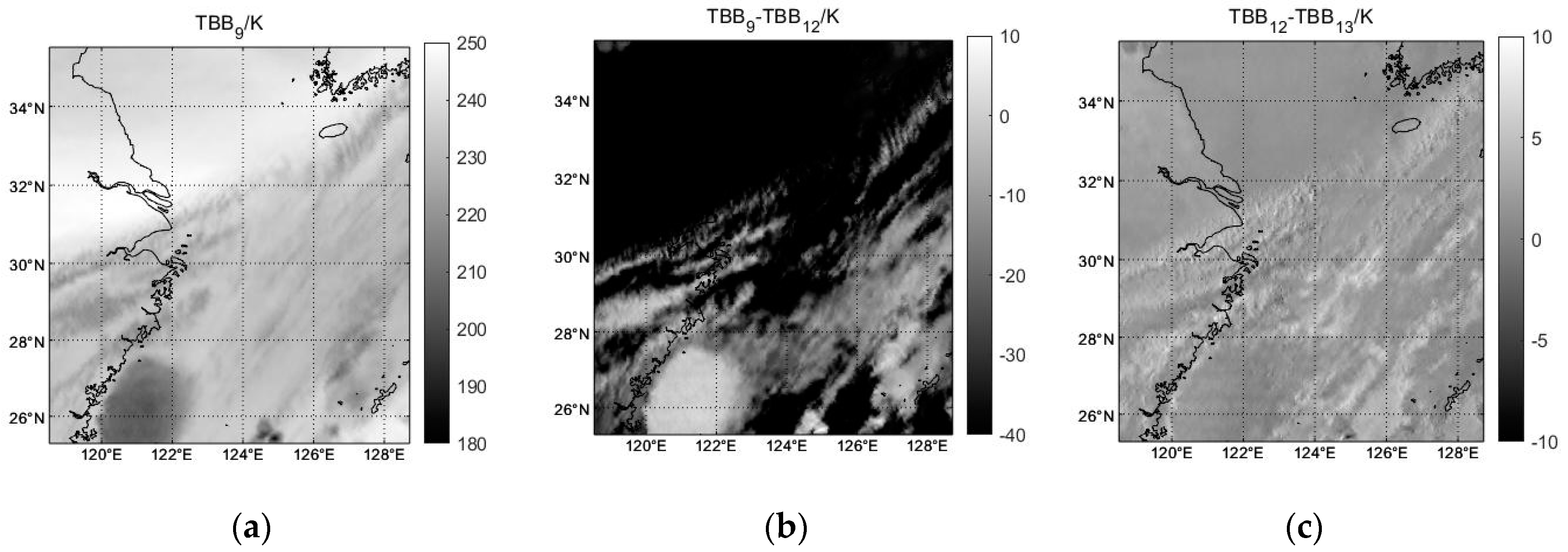
3.2.1. Analyze Spectral features

The 9th band (6.25 µm) of FY-4A is the water vapor band, and the 12th band (10.7 µm) and 13th band (12.0 µm) are long-wave infrared bands. Let the brightness temperature of a pixel in the satellite images of the 9th, 12th, and 13th bands with the same pixel position and at the same time be TBB9, TBB12, and TBB13, respectively. Through analysis, three spectral characteristic quantities are selected: brightness temperature at the ninth band TBB9, brightness temperature difference value TBB9−TBB12, and TBB12TBB13. Figure 7 shows the three spectral features selected in this paper for recognizing severe convective clouds.

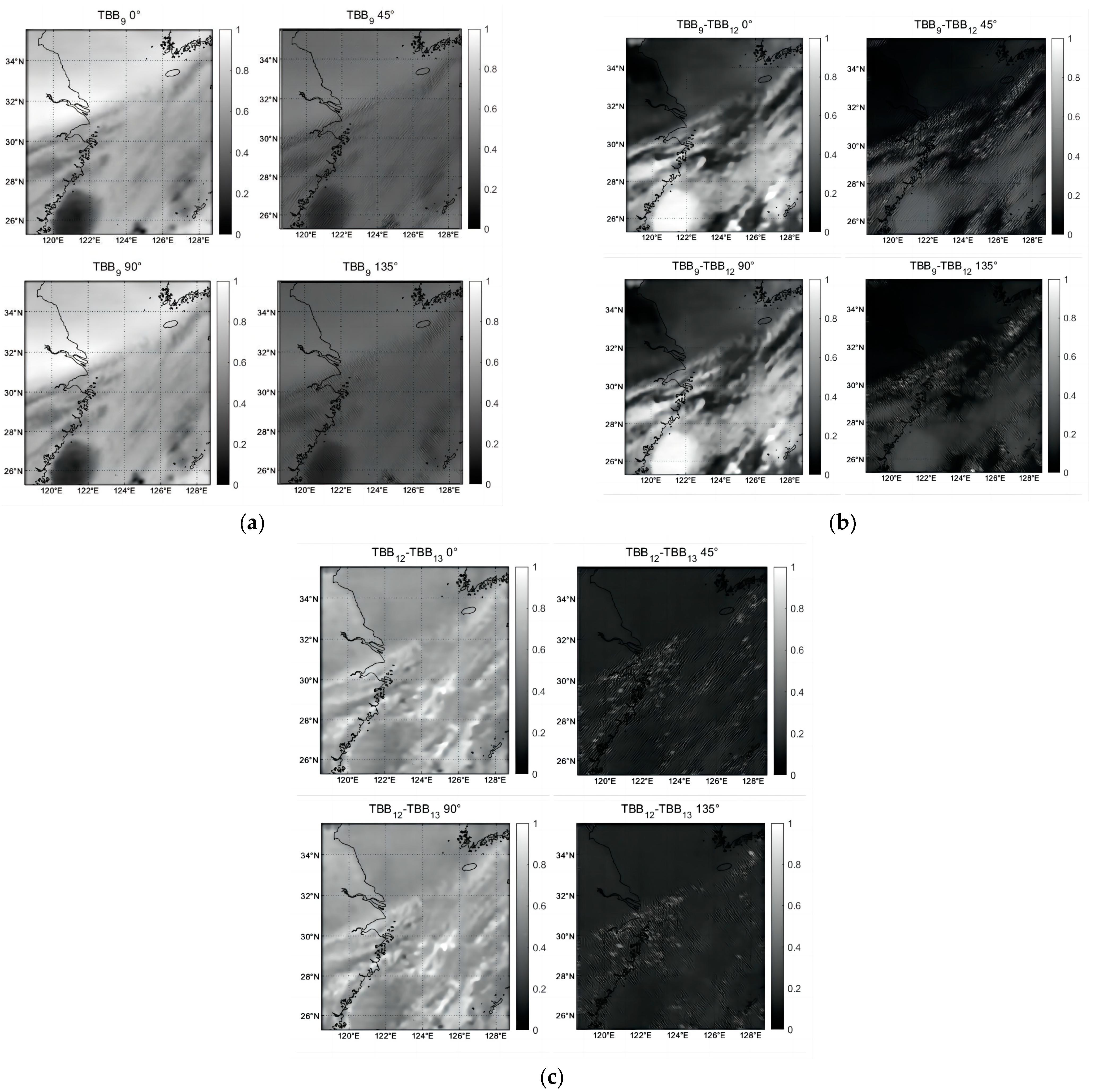
3.2.2. Extract Texture Features

Gabor transform was used to extract the texture features of severe convective cloud images in different directions. Gabor transform is a short-time window Fourier transform with a Gaussian window function [28], which aims to satisfy two-dimensional images’ locality in spatial and frequency domains. In two-dimensional image processing, the Gabor filter has good filtering performance, is similar to the human visual system, and has a good texture detection function [29]. The two-dimensional Gabor filtering function is as follows:
G ( x , y , f , θ ) = e x p { 1 2 [ ( x p S x ) 2 + ( y p S y ) 2 ] } × c o s ( 2 π f × x p )
where x p = x c o s θ + y s i n θ , y p = y c o s θ x s i n θ . S x and S y are the ranges of variables changing on the x and y axes, respectively, representing the size of the selected Gabor wavelet window; f is the frequency of the sine function; and G is the Gabor filtering function g ( x , y ) .
Figure 8 shows the texture features extracted by Gabor filter at 0°, 45°, 90°, and 135° directions.

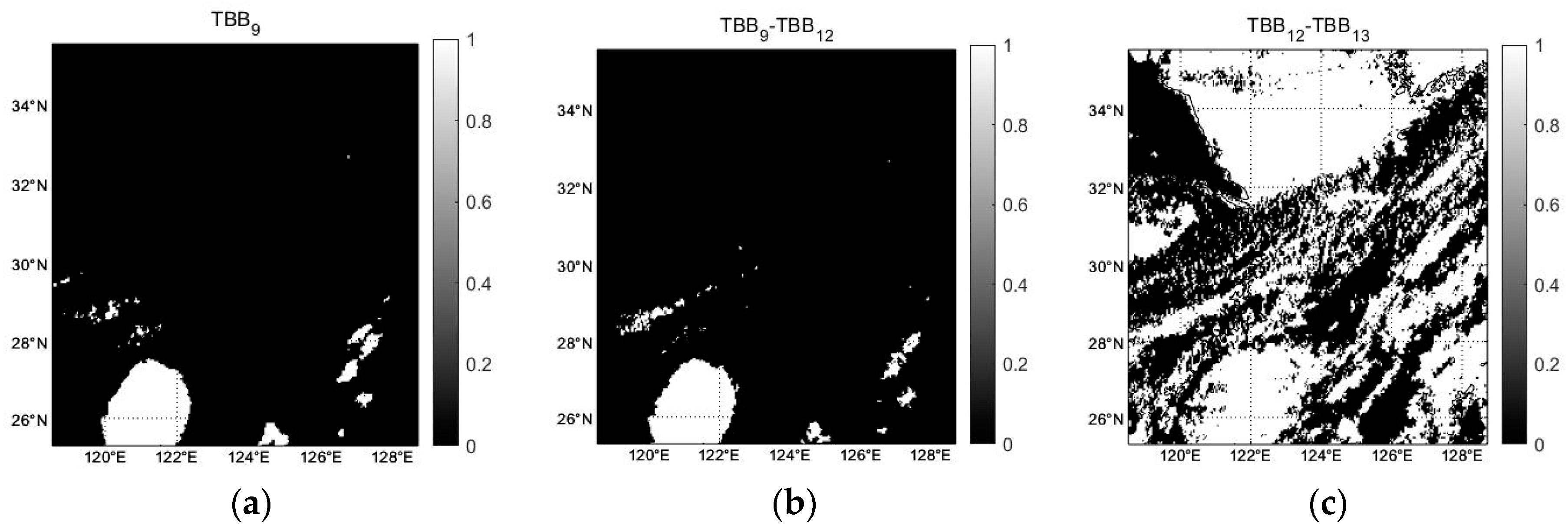
3.2.3. Image Binarization

The cloud clusters in which the brightness temperature of the water vapor channel is more than 220 K were removed, and the TBB9 spectral features were binarized, as shown in Figure 9a.
The brightness temperature difference TBB9−TBB12 was greater than −4 K in the water vapor-infrared window region and was used for the preliminary extraction of convective clouds. The spectral characteristics of TBB9−TBB12 were binarized, as shown in Figure 9b.
There were still cirrus and other noises in the convective cloud data preliminarily extracted by the brightness temperature difference of water vapor-infrared window, and the split-window brightness temperature difference method used in the experiments excluded noise such as partial cirrus clouds by selecting TBB12−TBB13 < 2 K as the threshold value, as shown in Figure 9c.

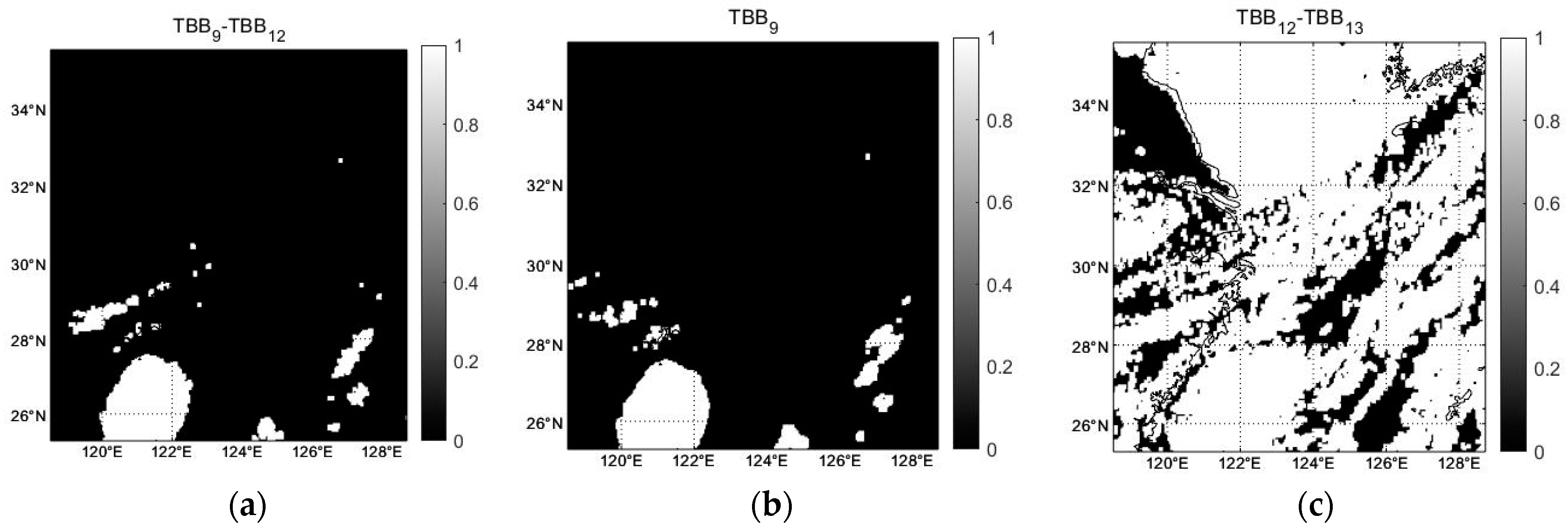
3.2.4. Closed Operations and Intersection Operations

(1)
A closed operation was carried out on the preliminary recognition results of severe convection by TBB9, TBB9−TBB12, and TBB12−TBB13, as shown in Figure 10.
(2)
Take the intersection operation of the two pictures in Figure 10a,b to obtain the labels needed for the final severe convection recognition, as shown in Figure 11.
Set the area threshold to 4, and the area with less than 4 pixels will be excluded from the binarized image, as shown in Figure 12.

3.3. Model Performance Evaluation Method

3.3.1. Model Performance Evaluation of Cloud Image Prediction

In order to quantitatively evaluate the prediction effect of the model, this study selected the evaluation indexes of peak signal-to-noise ratio (PSNR), root-mean-square error (RMSE), and correlation coefficient (R2). The calculation formulas are as follows:
P S N R = 10 l o g 10 ( M A X 2 M S E )  
R M S E = 1 M N i = 1 M j = 1 N [ I ( i , j ) K ( i , j ) ] 2
R 2 = 1 1 M N i = 1 M j = 1 N [ I ( i , j ) K ( i , j ) ] 2 1 M N i = 1 M j = 1 N [ I ( i , j ) ¯ K ( i , j ) ] 2  
where M A X 2 is the maximum possible value of a picture pixel. M and N are the height and width of the image, I ( i , j ) represents the pixel value of the i -th row and the j -th column in the observed image, and K ( i , j ) represents the pixel value of the i -th row and the j -th column in the model predicted image.

3.3.2. Model Performance Evaluation of Recognition of Severe Convective Cloud

To further validate the proposed model in this article, four evaluation metrics—accuracy, precision, recall, and F1-score—were used to quantitatively analyze the results of recognizing severe convective clouds. The calculation formulas for these four evaluation metrics are as follows:
a c c u r a c y = T P + T N T P + T N + F P + F N
p r e c i s i o n = T P T P + F P  
r e c a l l = T P T P + F N
F 1 S c o r e = 2 × p r e c i s i o n × r e c a l l p r e c i s i o n + r e c a l l

4. Results

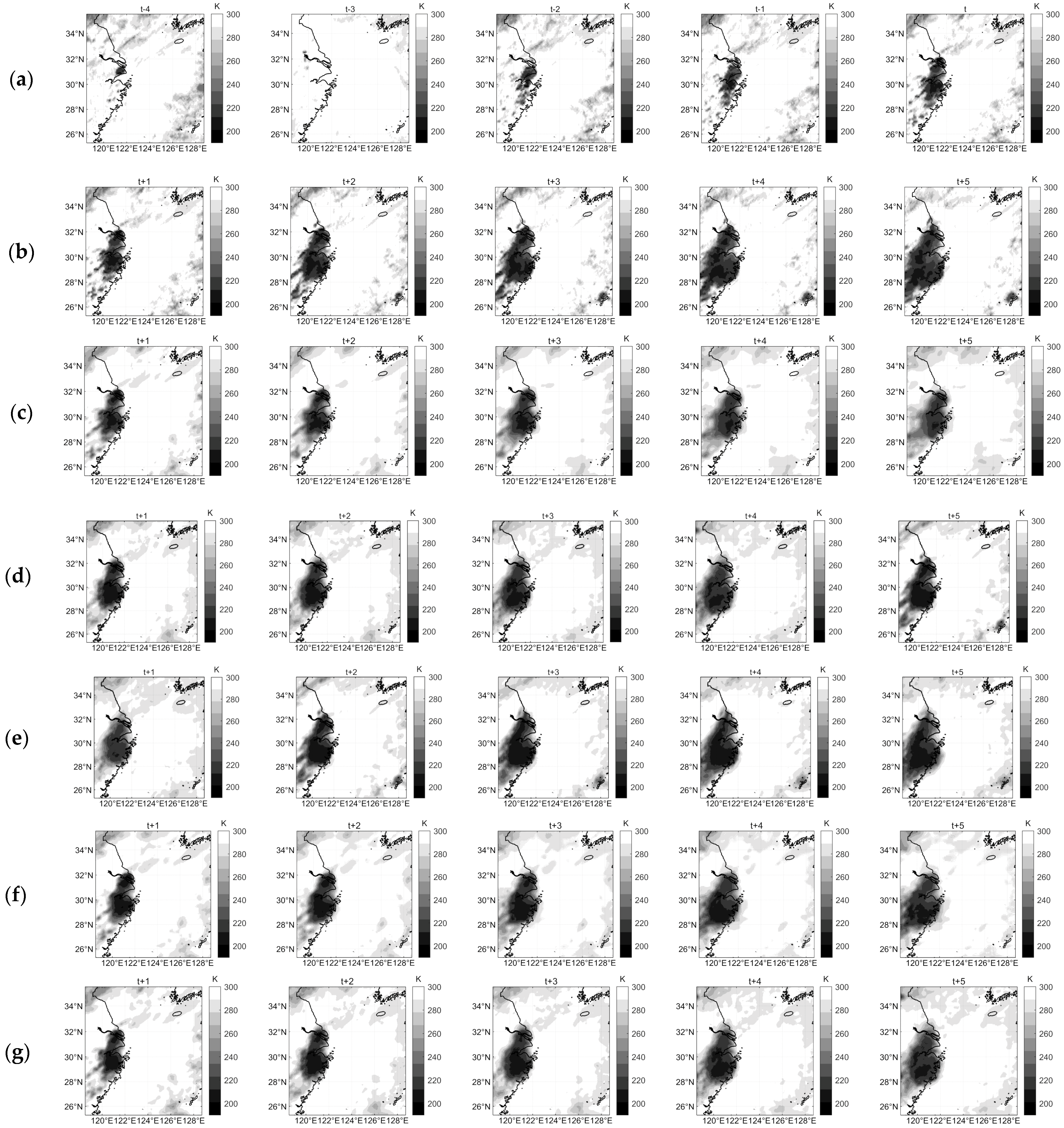
4.1. Cloud Image Prediction

4.1.1. Training

The length of each series was set to 5 time steps, and the time interval of each time node was 30 min; [ x t 4 , x t 3 , x t 2 , x t 1 , x t ] was the input data, [ x t + 1 , x t + 2 , x t + 3 , x t + 4 , x t + 5 ] was the output data, and t was the current moment. From June to September 2021 and 2022, 5000 time series were selected, of which 4000 time series were used as the training set, 500 time series as the validation set, and the remaining 500 data as the test set, for a total of 150 training epochs using the RMSprop optimizer.

4.1.2. Comparison of Cloud Image Prediction Models

Various deep learning models were used to compare the effect of cloud image prediction. The predicted results are shown in Figure 13.
It can be seen from Figure 13 that compared with the ARRU-Net model, the prediction image of other models was blurred. Only the general shape of the cloud could be seen; the fine-grained details of the clouds were significantly compromised, and the image became more and more blurred with time. However, the image predicted by the ARRU-Net model proposed in this study was closer to the label image, and the sharpness of the image was significantly higher than that of U-Net. With the change of time, the sharpness of the image changed little, and more cloud details could be predicted.
In order to evaluate the comparison results of this method with other models more objectively, the PSNR, RMSE, and R2 indexes of the four model prediction images on the test set were calculated, as shown in Figure 14. It can be seen from the figure that the prediction effect of ARRU-Net was better than that of other models. The average PSNR of the images predicted by ARRU-Net in the next five moments was more than 33 dB, the average RMSE at five moments was less than 7 K, and the average R2 at five moments was higher than 0.88. The ARRU-Net model achieved an average RMSE reduction of 1.3 K and a PSNR increase of 1.95 dB compared to U-Net in predicting the following five time steps on the test set. It is proved that this method can predict images that are clearer and more similar to the label images and have higher accuracy for long-term prediction.
We compared our method, ARRU-Net, with five other methods: Opticalflow-LK [30], DBPN [31], SRCloudNet [32], AFNO [33], and GAN+Mish+Huber [34]. Among the approaches, SRCloudNet, GAN+Mish+Huber, and AFNO were the newest state-of-the-art methods. As shown in Table 2, the ARRU-Net model outperformed some other methods.

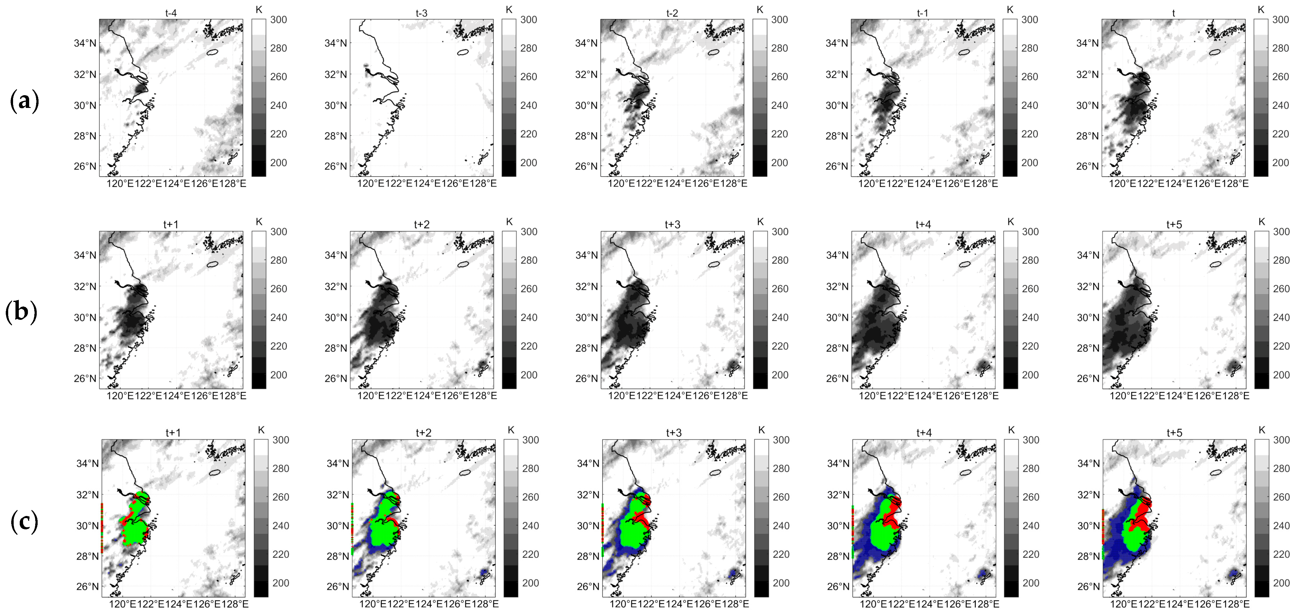
4.2. Recognition of Severe Convective Cloud Based on Cloud Image Prediction Sequence

4.2.1. Training

ARRU-Net and other models were used to recognize the severe convective clouds on cloud image prediction sequence. The models’ inputs were the predicted satellite cloud image sequence, and the outputs were the recognition result of the satellite cloud image sequence. The label images were formed according to the label-making method introduced in Section 3.2. The RMSprop optimizer was used for 150 training epochs.

4.2.2. Comparison of Recognition of Severe Convective Cloud Based on the Cloud Image Prediction Sequence

Figure 15 shows an example of recognition results for a predicted image sequence in a test set using the ARRU-Net model. The following is an example of the segmentation results of the predicted image sequence, where the gray base map is the predicted image, green represents the hit pixel, blue represents the missed image, and red represents the falsely detected pixel. The ARRU-Net model presented in this study had significantly more green hits than other models and had more red misses and fewer blue misses than other models.
Figure 15 shows the severe convection cloud recognition results of the ARRU-Net model and other models on the same test data for the predicted satellite cloud images. As can be seen from the Figure 16, the average accuracy and recall for cloud recognition were 97.62% and 83.34%, respectively, compared with the U-Net model, with a 2% increase in accuracy and a 4% increase in recall, indicating that this method can effectively eliminate cirrus clouds and improve the accuracy of severe convective cloud recognition. Therefore, quantitative and qualitative analysis show the apparent advantages of this method, and the ability of the ARRU-Net model to capture cloud features was improved, achieving more accurate severe convective cloud recognition.
We compared our method ARRU-Net with four deep-learning methods: GCN-LSTM [35], SegNet [36], GC–LSTM [37], and CNN + SVM/LSTM [38]. As shown in Table 3, the accuracy was 97.62%, which was much higher than that of other deep-learning methods.

5. Conclusions

The study was conducted to recognize severe convective clouds based on the FY-4A satellite image prediction sequence to provide more accurate guidance to mitigate the impact of severe convective weather. This study proposed the ARRU-Net model for predicting the following 2.5 h of satellite cloud images and recognizing convective clouds within them. Based on the U-Net network with the attention mechanism, the recurrent convolution, and the residual module, a new model was proposed, named ARRU-Net, for the recognition of severe convective clouds using the cloud image prediction sequence from FY-4A data. The characteristic parameters used to recognize severe convective clouds in this study were brightness temperature values TBB9, temperature difference values TBB9−TBB12 and TBB12−TBB13, and texture features based on spectral characteristics.
The results of the experiments indicated that the proposed method surpassed other comparative models. The RMSE, PSNR, and R2 of the predicted results were 5.48 K, 35.52 dB, and 0.92, respectively. The ARRU-Net model achieved an average RMSE reduction of 1.3 K and a PSNR increase of 1.95 dB compared to U-Net in predicting the following five time steps on the test set. The average accuracy and recall for cloud recognition were 97.62% and 83.34%, respectively, compared with the U-Net model, with a 2% increase in accuracy and a 4% increase in recall, indicating that this method can effectively eliminate cirrus clouds and improve the accuracy of severe convective clouds recognition.
Despite the promising results of this study, the model’s performance in predicting cloud images decreased over time. This was due to a sparse data, which can cause significant changes in the objects between adjacent images. Consequently, the prediction and segmentation of longer-term and small-scale convective clouds were affected. Further research is necessary to enhance the predicted images’ resolution and improve long-term sequence prediction accuracy.

Author Contributions

Conceptualization, X.Y. and Y.L.; methodology, Q.C., X.Y. and M.C.; software, Q.C. and X.Y.; investigation, X.Y. and Y.L.; writing—original draft preparation, Q.C.; writing—review and editing, X.Y., Y.L. and Q.X.; supervision, Q.X. and P.Z. All authors have read and agreed to the published version of the manuscript.

Funding

This research was funded by Laoshan Laboratory science and technology innovation projects, grant number No. LSKJ202201202, the Hainan Key Research and Development Program, grant number No. ZDYF2023SHFZ089, Fundamental Research Funds for the Central Universities, grant number No. 202212016 and the Hainan Provincial Natural Science Foundation of China, grant number No. 122CXTD519.

Data Availability Statement

Not applicable.

Acknowledgments

The authors would like to thank the China National Satellite Meteorological Center, which is freely accessible to the public.

Conflicts of Interest

The authors declare no conflict of interest.

References

  1. Gernowo, R.; Sasongko, P. Tropical Convective Cloud Growth Models for Hydrometeorological Disaster Mitigation in Indonesia. Glob. J. Eng. Technol. Adv. 2021, 6, 114–120. [Google Scholar] [CrossRef]
  2. Gernowo, R.; Adi, K.; Yulianto, T. Convective Cloud Model for Analyzing of Heavy Rainfall of Weather Extreme at Semarang Indonesia. Adv. Sci. Lett. 2017, 23, 6593–6597. [Google Scholar] [CrossRef]
  3. Sharma, N.; Kumar Varma, A.; Liu, G. Percentage Occurrence of Global Tilted Deep Convective Clouds under Strong Vertical Wind Shear. Adv. Space Res. 2022, 69, 2433–2442. [Google Scholar] [CrossRef]
  4. Jamaly, M.; Kleissl, J. Robust cloud motion estimation by spatio-temporal correlation analysis of irradiance data. Sol. Energy 2018, 159, 306–317. [Google Scholar] [CrossRef]
  5. Dissawa, D.M.L.H.; Ekanayake, M.P.B.; Godaliyadda, G.M.R.I.; Ekanayake, J.B.; Agalgaonkar, A.P. Cloud motion tracking for short-term on-site cloud coverage prediction. In Proceedings of the 2017 Seventeenth International Conference on Advances in ICT for Emerging Regions (ICTer), Colombo, Sri Lanka, 6–9 September 2017; pp. 1–6. [Google Scholar]
  6. Shakya, S.; Kumar, S. Characterising and predicting them ovement of clouds using fractional-order optical flow. IET Image Process. 2019, 13, 1375–1381. [Google Scholar] [CrossRef]
  7. Son, Y.; Zhang, X.; Yoon, Y.; Cho, J.; Choi, S. LSTM–GAN Based Cloud Movement Prediction in Satellite Images for PV Forecast. J. Ambient Intell. Humaniz. Comput. 2023, 14, 12373–12386. [Google Scholar] [CrossRef]
  8. Xu, Z.; Du, J.; Wang, J.; Jiang, C.; Ren, Y. Satellite image prediction relying on GAN and LSTM neural networks. In Proceedings of the ICC 2019-2019 IEEE International Conference on Communications (ICC), Shanghai, China, 20–24 May 2019; pp. 1–6. [Google Scholar]
  9. Bo, M.; Ning, Y.; Chenggang, C.; Jing, C.; Peifeng, X. Cloud Position Forecasting Based on ConvLSTM Network. In Proceedings of the 2020 5th International Conference on Power and Renewable Energy (ICPRE), Shanghai, China, 12–14 September 2020; pp. 562–565. [Google Scholar]
  10. Harr, T.J.; Vonder, T.H. The Diurnal Cycle of West Pacific Deep Convection and Its Relation to the Spatial and Temporal Variation of Tropical MCS. J. Atmos. Sci. 1999, 56, 3401–3415. [Google Scholar]
  11. Fu, R.; Del, A.D.; Rossow, W.B. Behavior of Deep Convection Clouds in the Tropical Pacific Deduced from ISCCP Radiances. J. Clim. 1990, 3, 1129–1152. [Google Scholar] [CrossRef]
  12. Vila, D.A.; Machado, L.A.T.; Laurent, H. Forecast and Tracking of Cloud Clusters Using Satellite Infrared Imagery: Methodology and Validation. Weather Forecast. 2008, 23, 233–244. [Google Scholar] [CrossRef]
  13. Mecikalski, J.R.; Bedka, K.M. Forecasting Convective Initiation by Monitoring the Evolution of Moving Cumulus in Daytime GOES Imagery. Mon. Weather Rev. 2006, 134, 49–78. [Google Scholar] [CrossRef]
  14. Jirak, I.L.; Cotton, W.R.; McAnelly, R.L. Satellite and Radar Survey of Mesoscale Convective System Development. Mon. Weather Rev. 2003, 131, 2428–2449. [Google Scholar] [CrossRef]
  15. Sun, L.-X.; Zhuge, X.-Y.; Wang, Y. A Contour-Based Algorithm for Automated Detection of Overshooting Tops Using Satellite Infrared Imagery. IEEE Trans. Geosci. Remote Sens. 2019, 57, 497–508. [Google Scholar] [CrossRef]
  16. Mitra, A.K.; Parihar, S.; Peshin, S.K.; Bhatla, R.; Singh, R.S. Monitoring of Severe Weather Events Using RGB Scheme of INSAT-3D Satellite. J. Earth Syst. Sci. 2019, 128, 36. [Google Scholar] [CrossRef]
  17. Welch, R.M.; Sengupta, S.K.; Goroch, A.K.; Rabindra, P.; Rangaraj, N.; Navar, M.S. Polar Cloud and Surface Classification Using AVHRR Imagery: An Intercomparison of Methods. J. Appl. Meteorol. 1992, 31, 405–420. [Google Scholar] [CrossRef]
  18. Zinner, T.; Mannstein, H.; Tafferner, A. Cb-TRAM: Tracking and Monitoring Severe Convection from Onset over Rapid Development to Mature Phase Using Multi-Channel Meteosat-8 SEVIRI Data. Meteorol. Atmos. Phys. 2008, 49, 181–202. [Google Scholar] [CrossRef]
  19. Bedka, K.; Brunner, J.; Dworak, R.; Feltz, W.; Otkin, J.; Greenwald, T. Objective Satellite-Based Detection of Overshooting Tops Using Infrared Window Channel Brightness Temperature Gradients. J. Appl. Meteorol. Climatol. 2010, 49, 181–202. [Google Scholar] [CrossRef]
  20. Yang, J.; Zhang, Z.; Wei, C.; Lu, F.; Guo, Q. Introducing the New Generation of Chinese Geostationary Weather Satellites, Fengyun-4. Bull. Am. Meteorol. Soc. 2017, 98, 1637–1658. [Google Scholar] [CrossRef]
  21. Ronneberger, O.; Fischer, P.; Brox, T. Convolutional networks for biomedical image segmentation. In Proceedings of the Medical Image Computing and Computer-Assisted Intervention–MICCAI 2015 Conference Proceedings, Munich, Germany, 5–9 October 2015. [Google Scholar]
  22. Lai, S.; Xu, L.; Liu, K.; Zhao, J. Recurrent convolutional neural networks for text classification. In Proceedings of the AAAI Conference on Artificial Intelligence, Austin, TX, USA, 25–30 January 2015; Volume 29. [Google Scholar]
  23. He, K.; Zhang, X.; Ren, S.; Sun, J. Deep Residual Learning for Image Recognition. In Proceedings of the Conference on Computer Vision and Pattern Recognition, Las Vegas, NV, USA, 27–30 June 2016; pp. 770–778. [Google Scholar]
  24. Alom, M.Z.; Yakopcic, C.; Taha, T.M.; Asari, V.K. Nuclei Segmentation with Recurrent Residual Convolutional Neural Networks Based U-Net (R2U-Net). In Proceedings of the NAECON 2018-IEEE National Aerospace and Electronics Conference, Dayton, OH, USA, 23–26 July 2018; pp. 228–233. [Google Scholar]
  25. Liang, M.; Hu, X. Recurrent Convolutional Neural Network for Object Recognition. In Proceedings of the Conference on Computer Vision and Pattern Recognition, Boston, MA, USA, 7–12 June 2015; pp. 3367–3375. [Google Scholar]
  26. Orhan, E.; Pitkow, X. Skip Connections Eliminate Singularities. In Proceedings of the International Conference on Learning Representations, Vancouver, BC, Canada, 30 April–3 May 2018; Volume 24, pp. 183–243. [Google Scholar]
  27. He, K.; Zhang, X.; Ren, S.; Sun, J. Identity Mappings in Deep Residual Networks. In Proceedings of the Computer Vision–ECCV 2016: 14th European Conference, Amsterdam, The Netherlands, 11–14 October 2016; pp. 630–645. [Google Scholar]
  28. Jain, A.K.; Farrokhnia, F. Unsupervised Texture Segmentation Using Gabor Filters. Pattern Recognit. 1991, 24, 1167–1186. [Google Scholar] [CrossRef]
  29. Knowlton, K.; Harmon, L. Computer-Produced Grey Scales. Comput. Graph. Image Process. 1972, 1, 1–20. [Google Scholar] [CrossRef]
  30. Bouguet, J.Y. Pyramidal implementation of the affine Lucas Kanade feature tracker description of the algorithm. Intel Corp. 2001, 1, 4. [Google Scholar]
  31. Haris, M.; Shakhnarovich, G.; Ukita, N. Deep back-projection networks for super-resolution. In Proceedings of the Conference on Computer Vision and Pattern Recognition, Salt Lake City, UT, USA, 18–23 June 2018; pp. 1664–1673. [Google Scholar]
  32. Zhang, J.; Yang, Z.; Jia, Z.; Bai, C. Superresolution imaging with a deep multipath network for the reconstruction of satellite cloud images. Earth Space Sci. 2021, 10, 1029–1559. [Google Scholar] [CrossRef]
  33. Guibas, J.; Mardani, M.; Li, Z.; Tao, A.; Anandkumar, A.; Catanzaro, B. Proceedings of the Adaptive Fourier neural operators: Efficient token mixers for transformers. International Conference on Learning Representations, Virtual Event, 25–29 April 2022; pp. 1–15. [Google Scholar]
  34. Wang, R.; Teng, D.; Yu, W. Improvement and Application of GAN Models for Time Series Image Prediction—A Case Study of Time Series Satellite Nephograms. Res. Sq. 2022, 29, 403–417. [Google Scholar]
  35. Zhou, J.; Xiang, J.; Huang, S. Classification and Prediction of Typhoon Levels by Satellite Cloud Pictures through GC–LSTM Deep Learning Model. Sensors 2020, 20, 5132. [Google Scholar] [CrossRef]
  36. Badrinarayanan, V.; Kendall, A.; Cipolla, R. Segnet: A deep convolutional encoder-decoder architecture for image segmentation. IEEE Trans. Pattern Anal. Mach. Intell. 2017, 39, 2481–2495. [Google Scholar] [CrossRef]
  37. Tao, R.; Zhang, Y.; Wang, L.; Cai, P.; Tan, H. Detection of precipitation cloud over the tibet based on the improved U-net. Comput. Mater. Contin. 2020, 5, 115–118. [Google Scholar] [CrossRef]
  38. Heming, J.T.; Prates, F.; Bender, M.A.; Bowyer, R.; Cangialosi, J.; Caroff, P.; Coleman, T.; Doyle, J.D.; Dube, A.; Faure, G. Review of recent progress in tropical cyclone track forecasting and expression of uncertainties. Trop. Cyclone Res. Rev. 2019, 8, 181–218. [Google Scholar] [CrossRef]
Figure 1. Illustration of the selected area and the observation area of the FY-4A satellite.
Remotesensing 15 04612 g001
Figure 2. Examples of FY-4A AGRI imager all-channel observation images.
Remotesensing 15 04612 g002
Figure 3. The proposed ARRU-Net model structure with recurrent residual and attention modules: (a) encoder; (b) decoder; (c) recurrent residual convolutional units.
Remotesensing 15 04612 g003
Figure 4. Attention mechanism structure of the proposed ARRU-Net model.
Remotesensing 15 04612 g004
Figure 5. Two kinds of convolutional block: (a) a basic unit of the U-Net convolution; (b) the recurrent convolution of the proposed ARRU-Net model.
Remotesensing 15 04612 g005
Figure 6. Residual connection structure of the proposed ARRU-Net model.
Remotesensing 15 04612 g006
Figure 7. Three spectral feature images: (a) brightness temperature value TBB9; (b) brightness temperature difference value TBB9−TBB12; (c) brightness temperature difference value TBB12−TBB13.
Remotesensing 15 04612 g007
Figure 8. Three texture features extracted by Gabor filter at 0°, 45°, 90°, and 135° directions. (a) TBB9; (b) TBB9−TBB12; (c) TBB12−TBB13.
Remotesensing 15 04612 g008
Figure 9. Image binarization: (a) brightness temperature of the water vapor channel TBB9 < 220 K; (b) brightness temperature difference TBB9−TBB12 > −4 K; (c) brightness temperature difference of water vapor-infrared window TBB12−TBB13 < 2 K.
Remotesensing 15 04612 g009
Figure 10. The preliminary recognition results of severe convection after closed operation: (a) TBB9; (b) TBB9−TBB12; (c) TBB12−TBB13.
Remotesensing 15 04612 g010
Figure 11. The image of recognition result after intersection operation of Figure 10a,b.
Remotesensing 15 04612 g011
Figure 12. The image of recognition result after area threshold: (a) original image; (b) the final label image.
Remotesensing 15 04612 g012
Figure 13. Comparison of the results of cloud image prediction models: (a) input; (b) label; (c) U-Net; (d) ConvLSTM; (e) 3DCNN; (f) U-Net+Residual+Recurrent; (g) ARRU-Net.
Remotesensing 15 04612 g013
Figure 14. Model performance evaluation of cloud image prediction results: (a) PSNR; (b) R2; (c) RSME.
Remotesensing 15 04612 g014
Figure 15. Comparison of the results of recognition of severe convective cloud based on the cloud image prediction sequence: green represents the hit pixel, blue represents the missed image, and red represents the falsely detected pixel. (a) input; (b) label; (c) U-Net; (d) ConvLSTM; (e) 3DCNN; (f) U-Net+Residual+Recurrent; (g) ARRU-Net.
Remotesensing 15 04612 g015aRemotesensing 15 04612 g015b
Figure 16. Model performance evaluation of severe convective cloud image recognition results: (a) Accuracy; (b) Precision; (c) Recall; (d) F1-score.
Remotesensing 15 04612 g016
Table 1. FY4A AGRI Imager parameters by channel *.
Channel TypeCentral WavelengthSpectral BandwidthSpatial ResolutionMain Applications
VIS/NIR0.47 µm0.45–0.49 µm1 kmAerosol, visibility
0.65 µm0.55–0.75 µm0.5 kmFog, clouds
0.825 µm0.75–0.90 µm1 kmAerosol, vegetation
Shortwave IR1.375 µm1.36–1.39 µm2 kmCirrus
1.61 µm1.58–1.64 µm2 kmCloud, snow
2.25 µm2.1–2.35 µm2kmCloud phase, aerosol, vegetation
Midwave IR3.75 µm3.5–4.0 µm2 kmClouds, fire, moisture, snow
3.75 µm3.5–4.0µm4 kmLand surface
Water vapor6.25 µm3.5–4.0 µm2 kmUpper-level WV
7.1 µm3.5–4.0µm4 kmMidlevel WV
Longwave IR8.5 µm8.0–9.0 µm4 kmVolcanic, ash, cloud top, phase
10.7 µm3.5–4.0 µm4 kmSST, LST
12.0 µm3.5–4.0 µm4 kmClouds, low-level WV
13.5 µm3.5–4.0 µm4 kmClouds, air temperature
* Available online: http://www.sac347.org.cn/nsmc/cn/instrument/AGRI.html (accessed on 1 May 2022).
Table 2. Comparison of the performance of our model and other methods in cloud image prediction.
LiteratureSatelliteModelPSNR (dB)
Bouguet et al. [30]/Opticalflow-LK24.40
Haris et al. [31]/DBPN32.36
Zhang et al. [32]Himawari-8SRCloudNet32.43
Guibas et al. [33]/AFNO25.22
Wang et al. [34]FY-4A/AGRIGAN+Mish+Huber31.49
Our modelFY-4A/AGRIARRU-Net35.52
Table 3. Comparison of the performance of our model and other methods in cloud image recognition.
LiteratureSatelliteModelAccuracy
Zhou et al. [35]Himawari-8GCN-LSTM91.51%
Badrinarayanan et al. [36]/SegNet86.80%
Tao et al. [37]Himawari-8GC–LSTM95.12%
Heming et al. [38]/CNN + SVM/LSTM91.67%
Our modelFY-4A/AGRIARRU-Net97.62%
Disclaimer/Publisher’s Note: The statements, opinions and data contained in all publications are solely those of the individual author(s) and contributor(s) and not of MDPI and/or the editor(s). MDPI and/or the editor(s) disclaim responsibility for any injury to people or property resulting from any ideas, methods, instructions or products referred to in the content.

