Article

Estimation of Tropical Cyclone Intensity via Deep Learning Techniques from Satellite Cloud Images

1
Research Center for Wind Engineering and Engineering Vibration, Guangzhou University, Guangzhou 510006, China
2
School of Computer Science and Cyber Engineering, Guangzhou University, Guangzhou 510006, China
3
Hong Kong Observatory, Hong Kong 999077, China
*
Author to whom correspondence should be addressed.
Remote Sens. 2023, 15(17), 4188; https://doi.org/10.3390/rs15174188
Submission received: 2 August 2023 / Revised: 23 August 2023 / Accepted: 24 August 2023 / Published: 25 August 2023
(This article belongs to the Special Issue Analysis of Satellite Cloud Images via Deep Learning Techniques)

Abstract

:
Estimating the intensity of tropical cyclones (TCs) is usually involved as a critical step in studies on TC disaster warnings and prediction. Satellite cloud images (SCIs) are one of the most effective and preferable data sources for TC research. Despite the great achievements in various SCI-based studies, accurate and efficient estimation of TC intensity still remains a challenge. In recent years, machine learning (ML) techniques have gained fast development and shown significant potential in dealing with big data, particularly with images. This study focuses on the objective estimation of TC intensity based on SCIs via a comprehensive usage of some advanced deep learning (DL) techniques and smoothing methods. Two estimation strategies are proposed and examined which, respectively, involve one and two functional stages. The one-stage strategy uses Vision Transformer (ViT) or Deep Convolutional Neutral Network (DCNN) as the regression model for directly identifying TC intensity, while the second strategy involves a classification stage that aims to stratify SCI samples into a few intensity groups and a subsequent regression stage that specifies the TC intensity. Further efforts are made to improve the estimation accuracy by using smoothing manipulations (via four specific smoothing techniques) in the scenarios of the aforementioned two strategies and their fusion. Results show that DCNN performs better than ViT in the one-stage strategy, while using ViT as the classification model and DCNN as the regression model can result in the best performance in the two-stage strategy. It is interesting that although the strategy of singly using DCNN wins out over any concerned two-stage strategy, the fusion of the two strategies outperforms either the one-stage strategy or the two-stage strategy. Results also suggest that using smoothing techniques are beneficial for the improvement of estimation accuracy. Overall, the best performance is achieved by using a hybrid strategy that consists of the one-stage strategy, the two-stage strategy and smoothing manipulation. The associated RMSE and MAE values are 9.81 kt and 7.51 kt, which prevail over those from most existing studies.

1. Introduction

TCs are highly destructive natural disasters, and accurate assessment of their activities are essential for the prevention and reduction of TC disasters. Among all TC parameters, intensity is perhaps the most complex one as it not only physically depends upon lots of factors, such as background environment, TCs’ inner structures and their interactions, but also capriciously varies with location and time sometimes. Consequently, research on TC intensity has been a major priority in the fields of meteorology and oceanography. However, due to the vast scale of TC structures and their complicated evolution in spatial-temporal domain during the life-cycle, it remains a challenge to characterize TC intensity via earth-based instruments especially before TCs’ landfall.
With the help of ever developing equipment and technology, humans can now obtain more credible information of TCs even over seas from reconnaissance aircrafts and airborne devices. However, such instruments are too expensive for routine usage at a global scale, which restricts the coverage of associated observations in terms of space and time. By contrast, satellite remote sensing data, in particular SCIs, provide abundant information of TCs and accompanied background environment over vast oceans in an uninterrupted way. As a result, they have been widely used for both academic studies and application practices.
Continuous efforts have been made to estimate TC intensity from SCIs. The Dvorak technique, initially documented by Dvorak, is a set of TC analytical methods that identify TC fingerprints and produce preliminary judgments of TC intensity, and then utilize different cloud textures and change patterns to refine final estimations [1]. This technique has been further developed such as by Velden et al. [2,3,4]. Many other estimation methods have also been proposed since the beginning of this century, including the fixed-intensity Advanced Microwave Sounding Unit (AMSU) method [5], manual techniques for intensity estimation using SSM/I images [6], a near-real-time technique for characterizing the shape and dynamics of TCs and correlating them with TC intensity [7], and a TC intensity estimation method using spatial characteristic analogue in satellite data [8]. Moreover, studies on the deviation angle variation (DAV) method for estimating TC intensity using geostationary infrared (IR) brightness and temperature data [9], estimation of wind speed at flight altitude using conventional TC information and IR satellite images [10], multiple linear regression models for estimating TC intensity by IR satellite images [11], and empirical estimation of TC intensity by the SATCON weighted consensus algorithm [12] have been conducted as well.
Despite their widespread use in meteorology, the aforementioned techniques face some challenges when applied in practice. Typically, many techniques involve experience-based manipulations, which make the estimations tend to suffer from low efficiency and subjective errors. Therefore, there is a need to develop high-precision and objective methods for estimating TC intensity.
In recent years, machine learning (ML) techniques have gained fast development [13,14] and shown significant potential in dealing with many meteorological issues [15,16,17,18]. Among various ML techniques, the convolutional neural network (CNN) has attracted more and more attention for SCI-based estimation of TC intensity since, as an abstract feature extraction technology, it is capable of retrieving highly generalized information of TCs as well as identifying and classifying complex TC images [19,20]. For example, Combinido et al. [21] examined the performance of the VGG19 model driven by grayscale infrared (IR) images. Wimmers et al. [22] used 2D-CNN approach based on satellite passive microwave imagery. Chen et al. [23] built a CNN-TC regression model by taking into account the domain knowledge of meteorologists. Wang et al. [24] developed a CNN-based model with the help of H-8 geostationary satellite IR imagery. Zhang et al. [25] proposed a two-branch CNN model on the basis of IR and water vapor (WV) images. Lee et al. [26] further employed 3D-CNN to investigate the correlation between multi-spectral geostationary satellite images and TC intensity.
Another ML technique that varies significantly from CNN and its derivatives is Transformer, which currently dominates in the field of natural language processing (NLP). While CNN is operationally based on convolution calculations (which are good at capturing local features), Transformer is established on the basis of self-attention mechanism. This completely different mechanism enables Transformer to extract global features from longer sequences and improve computational efficiency through performing parallel computation during training and inference. In light of the striking success of Transformer in NLP, Dosovitskiy et al. [27] expanded it to the vision field and proposed Vision Transformer (ViT). Since its debut, ViT has achieved remarkable success in the vision field, outperforming most existing CNN models [28]. Undoubtedly, ViT has significant potential in meteorological remote sensing. In fact, Bi et al. [29] demonstrated that training ViT models with large amounts of reanalysis data can generate better results than those from numerical weather prediction (NWP). However, to the authors’ best knowledge, no studies have been reported on ViT-aided estimation of TC intensity.
It should be noted that the performance of ML models markedly depends on the quality and amount of input data, and it is not uncommon that a model performs well for some cases whilst it becomes degraded for others. Therefore, a cluster of ML techniques may be adopted concurrently to exert hybrid-related advantages.
This study focuses on ML-aided estimation of TC intensity based on SCIs. ViT is adopted for the first time to estimate TC intensity and its performance is examined through comparison with CNN. More importantly, special efforts are made to improve the estimation accuracy by comprehensive usage of multiple hybrid strategies. The remainder of the article is organized as follows. After an introduction of the datasets, data pre-processing and evaluation methods in Section 2, detailed performance of each ML model and ML-aided strategy is presented and discussed in Section 3. Main findings and conclusions are summarized in Section 4.

2. Methodology Statement

The adopted methodology is depicted in Figure 1, which mainly consists of the following four links: obtaining SCIs from open-source databases, conducting pre-processing manipulations (i.e., data augmentation and segmentation), training and validating different models, as well as analyzing and comparing estimation results.
Two basic DL-aided strategies are utilized to estimate TC intensity (in terms of maximum sustained wind, or MSW): the one-stage strategy that uses ViT or DCNN as the regression model for directly identifying MSW, and the two-stage strategy which involves a classification stage that aims to stratify SCI samples into a few intensity groups and a subsequent regression stage that specifies MSW. Further efforts are made to improve the estimation accuracy by using smoothing manipulations (via 4 techniques) in the scenarios of the two basic strategies and their fusion (i.e., a hybrid strategy).
The primary idea behind the two basic strategies lies in that input SCI samples are often unevenly distributed in varied intensity groups. While the groups containing more credible samples tend to generate ideally parameterized models and better estimation results, those with fewer samples are likely to suffer from insufficiently training and inferior model performance. Thus, it is expected that the two-stage strategy is helpful for minimizing the negative effects on those fewer-sample-featured groups caused by the “resourceful” groups.
Different from the above idea which tries to improve the estimation results during the identifying process (or simply, process-oriented), smoothing manipulation aims to refine the final results through the fusion of outputs from varied DL models or those from the same model but at different time steps (or result-oriented).

2.1. Datasets

2.1.1. Data Sources

The SCI data are derived from the Archives of Weather Home, Kochi University, Japan (http://weather.is.kochi-u.ac.jp/archive-e.html, accessed on 30 July 2022), which were captured by geostationary satellites “Himawari-8” and “MTSAT-1R” over the Northwest Pacific Ocean. Each grayscale infrared image (IR, 10.2–12.5 μm) contains 1800 × 1800 pixels that correspond to a geographic area of 70°N–20°S, 70°E–160°E. In total, 222,212 images are exploited in this study, which were taken at 1 h intervals during the life-cycles of 546 TCs from 2000 to 2021.
Corresponding label information, i.e., TC trajectory and intensity (defined as 10 min mean MSW; unit: knot or kt, 1 kt = 1.85 km/h = 0.514 m/s), is available from the Japan Meteorological Agency (JMA, Tokyo, Japan, https://www.data.jma.go.jp/, accessed on 15 June 2022). These labels are updated every 3 or 6 h. Note that the MSW values are provided in a form of integral multiples of 5 kt, and they would be marked as zero for MSW < 35 kt. JMA also stratifies TCs into 4 intensity categories according to MSW: typhoon (TY, 35–63 kt), strong typhoon (STY, 64-84 kt), very strong typhoon (VSTY, 85-104 kt), violent typhoon (VTY, >105 kt).
Besides the SCI datasets, this study also considers the reanalysis data estimated, respectively, via ADT (https://tropic.ssec.wisc.edu/real-time/adt/adt.html, accessed on 20 June 2022) and SATCON methods (https://tropic.ssec.wisc.edu/real-time/satcon/, accessed on 20 June 2022) for comparison purpose. These data are documented at 30 min intervals, and the TC intensity is expressed as the 1 min mean MSW which differs from the one issued by JMA. The method presented by Harper et al. [30] is adopted to convert between 1 min mean and 10 min mean MSWs.

2.1.2. Data Pre-Processing

There are two main tasks during this process: cropping TC structure from each original SCI, and data augmentation through image transformation.
The original SCIs cover a too large area with respect to a TC, which makes it difficult to identify TC intensity effectively via DL methods. Thus, it is required to extract the TC portion from the original image [31]. This can be fulfilled through automatically cropping manipulation in accordance with the best track data of targeted TCs, as shown in Figure 2a,b. After cropping, each image contains 400–500 pixels or spans 20°–25° along both longitude and latitude directions. The cropped SCIs are then standardized to a uniform size of 400 × 400 pixels. The standardized SCIs are further examined to ensure that TC structure is effectively covered in the processed images, and those with TC centers located beyond the images are discarded.
On the other hand, data augmentation aims to deal with the issue related to unbalanced distribution of SCI samples among different statues of TC intensity. Typically, the life-cycle of a TC consists of relatively longer periods of low-to-moderate intensity status and shorter episodes of high-intensity status. This unbalanced distribution of intensity status and therefore SCI samples can degrade the training quality for the models which usually require that the input samples should be evenly distributed along with the key targeted parameter (i.e., TC intensity). As demonstrated in Figure 2c–j, eight specific data augmentation manipulations, including image flipping, multi-angle rotation and noise addition, are employed in this study to collectively (i.e., regardless of intensity category) increase the number of TC samples. Images of TCs in the TY intensity category are then randomly down-sampled to improve the balance of samples among different intensity categories.
There are two points to be stressed. First, to ensure the objectivity and credibility of testing results, the dataset for testing (to be discussed in the following section) has only experienced cropping manipulation, whilst no operations for the aforementioned data augmentation have been conducted, as artificial transformations tend to destroy TCs’ morphological structures and make the processed SCIs physically meaningless. Second, although the process of data augmentation does moderate unbalanced-distribution-related issues, the samples of processed SCIs in categories with higher TC intensity levels are still lacking. By trial and error, better results can be achieved when the SCI samples are stratified into two categories: the one with MSW > 64 kt (referred to as STYS) and the one with MSW < 64 kt (referred to as TY). Thus, this stratification is exploited for the two-stage strategy.

2.1.3. Segmentation and Standardization

After pre-processing, the samples are segmented into three sets, i.e., training set, validation set and testing set, which are, respectively, used for training, validating and testing the DL networks. In total, 158,260 SCIs for 330 TCs from 2000 to 2013 are selected as the training set (refer to as TG, hereafter), 52,032 SCIs for 113 TCs from 2014 to 2017 are selected for validation (VG), and 11,921 SCIs for 103 TCs from 2018 to 2021 are selected for testing. Basic information of the three sets is tabulated in Table 1. Note that for the smoothing strategy, the testing set is further divided into two parts: one part (SCIs in 2020–2021) used to fit the smoothing models, while the other part (SCIs in 2018–2019) used to test the performance of smoothing models. It is essential to acknowledge that the practice of partitioning data by year introduces a certain degree of bias, given that more recent data tends to possess higher quality. However, even more crucially, this strategy guarantees complete independence between distinct datasets.
Meanwhile, both the pixel sizes and pixel values of SCIs for all the three sets are standardized to meet the input requirements of DL models. Each SCI is resized to contain 128 × 128 pixels for the DCNN model and 224 × 224 pixels for the ViT model, while the pixel values are normalized to be in the range of [–1, 1]. The normalization process is also helpful for enhancing the convergence during model training.

2.2. DCNN Model

CNN is a kind of ML network based on supervised learning. It has strong adaptability and is good at mining local features of data, extracting global training features and classification. However, simple CNN becomes unable to meet the universality and accuracy of various practical problems. Under such conditions, DCNN was proposed and has been utilized extensively.
As shown in Figure 3, a DCNN model usually consists of several functional modules/layers that can be combined in order and on request. Typical modules include the convolutional layer, pooling layer, dropout layer, and dense layer. The convolution layer contains multiple operational scanners, namely the convolution kernel, whose size is uniformly fixed within the layer. This layer is used to read the input information of the model and obtain various abstract features of the target through convolution calculation. The pooling layer filters matrix information through a series of pooling operations such as maximum pooling and average pooling. The dropout layer is used to maximize the efficiency of neural nodes by eliminating unimportant features. The dense layer is usually arranged at the end of the model, and is used to flatten the information of the previous layer as well as estimate the classification similarity by calculating a nonlinear function.
Functionally, the input and hidden layers cooperate to extract any potential features from the SCIs for identifying TC intensity, while the output layer conducts judgments and decisions according to the extracted results. It is clear that characterizing TC intensity essentially belongs to a regression problem. Therefore, the mean squared error (MSE) loss function (Equation (1)) and cross-entropy loss function (Equation (2)) are adopted herein to quantify the consistency of predictions against the actual results for the regression models and category models, respectively:
Loss MSE = 1 N i = 1 n ( y ^ i y i ) 2
L o s s   c r o s s e n t r o p y = 1 N i = 1 N c = 1 M y i c ln [ p ( y i c ) ]
where y i ^ represents the prediction of the true MSW values y i , N is the number of SCI samples, y i c is the label of the c-th classification (1 for positive judgments and 0 for negative judgments) for the i-th SCI, M is the number of categories, and p ( y i c ) denotes the probability of the prediction associated with y i c , which can be expressed via the softmax function:
p ( y i c ) = exp ( f y i c ) c = 1 C exp ( f y i c )
where f y i c is the original score of the model for prediction y i c , which is calculated by the output layer based on the 1000 × 1 dimensional output vector x (or the characteristic vector) from previous layers:
f y i c = W x + b
in which W (with dimensions 2 × 1000) represents the coefficient matrix which quantifies the weight for each element in x during the judging/prediction process, and b (with dimensions 2 × 1) is the bias vector.
Both W and b should be determined through training. In this study, the stochastic gradient descent (SGD) method is utilized to provide efficient estimation of the model parameters. SGD iteratively updates the W and b by computing gradients of the loss function and adjusting them in the direction that minimizes the loss. Moreover, the model involves a few hyperparameters, including the number of neural network nodes, the learning rate and epoch. These parameters are usually pre-set and adjusted empirically based on training results. Based on previous tests, the models in this study uses a learning rate of 0.001, with a batch size of 64–128.
The model generates a predicted value for each SCI, which ranges from 0 to 1. As the labels in the regression models are normalized using Min-Max scaling, the predictions from the model should be dimensionalized to the standard MSW scale through reverse normalization. For the classification model, a threshold of 0.5 is used to determine whether the SCI belongs to the STYS or TY category. Samples with predictions greater than 0.5 are classified as STYS, while those with a value less than or equal to 0.5 are classified as TY.

2.3. The ViT Model

Transformer is a novel neural network architecture that mainly utilizes self-attention mechanism to extract internal features. Its network architecture is primarily constructed around the attention mechanism. Based on the input information, the self-attention mechanism first generates three vectors, namely Query (Q), Key (K) and Value (V), through matrix transformation. Then, these vectors undergo multiple matrix operations and weightings, through which the most significant information can be enhanced while the less relevant information tends to be weakened. This is similar to the dot product operation of two vectors: the calculation result tends to be maximized for similar vectors, whilst it would be minimized for two orthogonal vectors. By repeating such attention operations, the model can output a set of feature vectors that selectively emphasize the salient information in the input.
ViT is actually an expanded version of the standard Transformer in the vision field. Figure 4 shows the inner structure of a ViT model [27]. There are two main functional modules: feature extraction module (i.e., Transformer Encoder) and classification calculation module (right part of the figure). A typical workflow for ViT involves the following several procedures: dividing the input images into blocks with a certain size, reassembling the divided image blocks into a sequence, transferring the combined results to the multi-head self-attention for feature extraction, and performing classification.
Taking Figure 4 as an example, the left part of the figure (i.e., Patch + Position Embedding and Transformer Encoder) corresponds to the realization process for feature extraction. The main function of “Patch + Position Embedding” is to divide the input image x, (x∈RH×W×C, where H/W and C represent the sizes of the image and the number of channels) into a number of sub-images xp, (xp∈RN × P^2 × C), where N(= 9 herein) represents the number of sub-images, P represents the size of sub-image. This processing is also termed as convolution, which uses a sliding window with a specific step size. These sub-images are then transformed into long vectors using a linear transformation. Each vector is combined with a position-encoded vector, as depicted in Figure 4, the number 1 to 9. This position encoding vector is learnable and can be adjusted automatically through training. Each sub-image vector with the position information is called a token. Notably, a special class (Cls) token is inserted at position 0 in Figure 4, which aggregates information from the entire input sequence into a vector for the classification task. After patching and Position Embedding, the input tensor is processed through the Transformer Encoder for computation. In the self-attentive computation of Transformer, each token in the input tensor is attention-weighted and summed over the other tokens to generate the corresponding contextual representation. Finally, after several Transformer cycles, the classification information vector is passed to the classification computation module for scoring and generating the final output.
z 0 = x class   ; x p 1 E ; x p 2 E ; L ; x p N E + E pos , E R P 2 × C × D , E pos   R ( N + 1 ) × D
z l = MSA LN z l 1 + z l 1 , l = 1 L
z l = MLP LN ( z l ) + z l l = 1 L
y = LN z L 0
Mathematically, the above process can be summarized as Equation (5), where xclass represents the class token vector, i.e., the asterisk of the yellow forms in Figure 4; x p N represents each sub-image, and E represents a linear projection layer (or the fully connected layer); x p N E represents sub-image vector after transformation; E pos represents the position coding information vector; while z 0 is the processed input of Transformer Encoder. Next, the operations in Equations (6) and (7) will be repeated L times, where MSA indicates the multi-head self-attention operation [32] of the Transformer, and MLP represents multi-layer perceptron operations. Furthermore, regularization is required before the operations, denoted by LN. In Equations (5)–(7), z l , z l , and z l 1 / z l 1 represent the result of multi-head self-attention calculation, the calculation result of a complete transformer block, and the corresponding residual connection, respectively. After several looped calculations, the output z L 0 (the final classification information vector) will be regularization by Equation (8), which is regarded as a feature of the entire image to carry out the classification or regression task.

2.4. Smoothing Methods

Four smoothing techniques are exploited to refine the estimation of TC intensity based on the output predictions from different DL models or the same model but at varied time steps: (i) linear fitting, which is a statistical method used to establish linear relationships between variables; (ii) Gradient Boosting (GB), which is a machine learning method that combines multiple weak predictive models [33]. It works by iteratively adding new models that predict the residuals of the previous models, and then combines them to obtain a final prediction; (iii) Random Forest (RF), which is another ML algorithm that builds multiple decision trees and combines their predictions to obtain the final result. Each decision tree is trained on a random subset of the data, and the final prediction is obtained by aggregating the predictions of all trees; (iv) multi-layer perceptron, which is an artificial neural network consisting of multiple layers of interconnected nodes or neurons, and it is a powerful ML method for learning complex patterns. This study utilizes estimates of frames at time t − 2, t − 1, and t to fit or smooth the final output. The specific steps include: (i) sequentially organizing the output outcomes of the DL model in accordance with their temporal sequence; (ii) using estimates from the current frames and the previous two frames as inputs for four smoothing methods. This generates smoothed estimates for the current TC intensity; (iii) replacing the DL model estimate with the smoothed estimate and repeating the process for the next time step. This is performed iteratively until all test data estimates are replaced by smoothed estimates.

2.5. Other Techniques

2.5.1. ADT

As an enhancement of the standard Dvorak technology (DT), ADT was developed on the basis of the combination of DT and other algorithms or models [3,4]. DT was originally proposed as a subjective method for TC intensity estimation based on satellite images. It first locates the center of TC and then provides the intensity of the TC activity through cloud model analysis. With the wide application of DT, increasing number of people improve the standard DT by introducing other technologies. In the latest version of ADT (ADT 9.0), statistical models and dynamic models were integrated to eliminate subjective factors. After objective positioning, ADT uses the statistical analysis results of all intensity range TC samples to obtain the intensity estimation value based on regression statistics for a certain TC. One of the biggest advantages of ADT is that it can be applied to every stage of the TC life cycle, which is difficult to achieve for other technologies.

2.5.2. SATCON

Advanced satellite consensus (SATCON) [12,34] combines ADT estimation with other methods for estimating TC intensity based on satellite remote sensing, including AMSU, SSMIS, and ATMS and finally develops into a global TC intensity ensemble estimation system. Specifically, SATCON utilizes statistical weighting methods to maximize the advantages (or minimize the disadvantages) of each type of technology and generates a consensus strength estimation for various TC structures. The statistical validation of this method indicates that it is technically equivalent to the DT used by most meteorological organizations; however, in some cases, the algorithm can outperform the DT, and the root mean square error of its intensity is also lower than that of most current techniques. In addition, this method has its advantages, such as alerting forecasters to rapid changes in TC intensity that traditional methods (such as DT) may be unable to capture. Although SATCON performs better than other methods for estimating TC intensity, it still has some limitations, especially for real-time applications, as the estimation always depends on certain satellite data. As a result, it fails to continuously work or to provide constant feedback in time.

2.6. Model Performance

The performance of regression models are usually evaluated the following statistical indices: root mean square error (RMSE), mean absolute error (MAE), and mean absolute percentage error (MAPE).
RMSE = 1 n j = 1 n ( p j o j ) 2
MAE = 1 n j = 1 n p j o j
MAPE = 100 % n j = 1 n p j o j o j
where p j represents the prediction (estimated values, which are similar to the variable y i ^ in Equation (1)) of observation values (true values, which are similar to the variable y i in Equation (1)) o j , and n represents the number of samples.
For the classification models in this study, the performance is qualified via precision (P), recall rate (R), and F1 score (F). Table 2 presents the confusion matrix which compiles the classifier results for calculating the PRF values. Here, NTP represents true positive prediction, NTN denotes true negative prediction, NFP refers to false positive prediction, and NFN stands for false negative prediction. It is clear from the definitions (Equations (12)–(15)) of PRF, P indicates the accuracy of positive predictions, R represents the percentage of correctly identified positive samples among all positive samples, while F1-score is used to evaluate the overall performance of the model as it provides the harmonic mean of P and R.
A c c u r a c y = N T P + N T N N T P + N T N + N F P + N F N
P r e c i s i o n = N T P N T P + N F P
Recall = N T P N T P + N F N
F 1 = 2 Recall × Pr e c i s i o n Recall + Pr e c i s i o n

2.7. Computational Platform

The DCNN model and supervised learning algorithms are coded using Python 3.7 with Keras 2.2.4 and Tensorflow 2.1.0 package. The model training was accomplished on an NVIDIA GeForce RTX 2080 Ti × 4 GPU and parallel computing management software CUDA (v10.1), acceleration library cuDNN (v7.6.0.64).

3. Results and Discussions

3.1. The One-Stage Strategy

Figure 5 illustrates the learning curves of the two regression models, i.e., DCNN and ViT, during the training (TG) and validating (VG) processes. As demonstrated, the DCNN model can be optimized rapidly, whereas ViT requires more epochs for optimization. Meanwhile, the minimum loss value of DCNN during validating is much less than the one of ViT. Based on these results, it can be tentatively concluded that DCNN outperforms ViT for the regression of TC intensity.
Since each epoch in Figure 5 corresponds to a parameterized model during the training and validating processes, we can select the best model according to the minimum value of the loss function from validating. Table 3 and Figure 6 summarize the overall performance of the best DCNN and ViT models. Again, it is seen that the DCNN model prevails over the ViT model. There are two possible reasons for this somewhat unexpected observation. First, ViT requires much more data to achieve an optimized status during training [27], while the amount of training set in this study is insufficient to further optimize the model parameters. Second, ViT contains many tricks and optimizations for classify problems, which however do not work for regression tasks.
Results in Figure 6 also indicate that both the DCNN and ViT models tend to underestimate the TC intensity for samples with high intensity levels. This trend is consistent with the fact that the number of SCI samples decreases with increasing TC intensity.
To further explore the above finding, Figure 7 examines the distribution of estimation errors (in terms of both absolute and relative errors, i.e., RMSE and MAPE) with geographic coordinate. To better understand the results exhibited in the figure, Figure 8 depicts the appearance probability of TC geneses and TCs with different intensity levels. From Figure 7, large RMSE values are basically located at: (i) Luzon peninsula and surrounding areas to its west/northwest where TCs (usually with high-intensity levels) are markedly influenced by landfall-related effects, (ii) southeast of the Northwest Pacific that is dominated by TC geneses, (iii) central south of the Northwest Pacific where both TC geneses and stronger TCs usually exist. By contrast, conditions for the relative error vary from those for RMSE significantly: almost all large MAPE values site around the periphery of TC-influenced areas where TCs tend to dissipate, whilst the central areas are featured by small values. There are also some patches where large values of both RMSE and MAPE exist, e.g., (155°E, 9°N). From Figure 8, the appearance probability of TCs at these locations is quite low.
The above findings can be reasonably explained by: (a) the morphological structures of TC geneses and TCs during or after landfall are much more complicated, whilst this complexity makes the input samples to be insufficient for training versatile DL models adequately; (b) the SCI samples of TCs with higher intensity levels are fewer than those with low-intensity-featured TCs, which degrades the model performance for stronger TCs. It is worth noting that the utilization of image transportation during data pre-processing can do reduce the negative influence caused by imbalanced distribution of samples to some extent. However, to improve the model substantially, more data that cover each typical condition are still required.

3.2. The Two-Stage Strategy

3.2.1. Performance of Classification Models

The first stage involved in the two-stage strategy aims to stratify input samples into a few intensity groups (two groups in this study, i.e., TY and STYS) via classification models. Thus, it is helpful to clarify the performance of these classification models for better understanding that of the two-stage strategy.
The learning curves for the classification models are presented in Figure 9. Table 4 compares the classification results via the DCNN and ViT models. The average values of prediction accuracy, recall rate, and F1 score for both models exceed 80%. Overall, the accuracy of DCNN is similar to the one reported by Wang [24] via CNN, while the ViT model performs better than DCNN especially for samples with higher intensity levels (by 2.5%). Both models perform noticeably better for TY category than for STYS, which is attributed to the fact that the former category contains larger amount of data and allows the models to be trained more efficiently.
To detail the performance of the two classification models, Table 5 and Table 6 exhibit the confusion matrix of predictions against the true labels. Results indicate that STY has the lowest recognition recall (66%). This phenomenon can be explained by the fact that STY (64–84 kt) and TY (34–63 kt) are two neighboring intensity categories, and there should be more samples belonging to varied categories but possessing much similar morphological features of the TC cloud, which makes the classification more challenging. Except for the STY category, the recognition recall for both models in other categories tends to increase with the increase of intensity level, which is consistent with the fact that the morphological characteristics of TCs from two farther-spaced intensity categories differ from each other more clearly.

3.2.2. Performance of the Two-Stage Strategy

Table 7 compares the performance of four specific scenarios for the two-stage strategy. Here, X_Y denotes a combination of X model for classification and Y model for regression, hereafter. The classification models are trained and optimized via the entire samples, while the regression models are treated similarly but via the samples associated with one of the two TC-intensity groups. The performance of the two-stage strategy is examined via the combined usage of the optimized classification model and regression model based on the testing dataset for the classification model.
As expected, ViT_DCNN achieves the best performance. However, comparison of the results in Table 3 and Table 7 reveals that the two-stage strategy does not surpass the one-stage strategy via DCNN. One major reason lies in that for the two-stage strategy, the misclassified samples at the first stage can bring in enlarged errors for the regression results at the second stage, and such errors cannot be diminished through better training the regression models.
Figure 10 shows the box plots of the estimation bias for each of the four JMA intensity categories via the four specific two-stage strategies. The red line represents median, while the grey points represent outlier. It is evident that the TC intensity of samples in STY, VSTY and VTY are all statistically underestimated. This systematic bias is primarily attributed to the insufficiency of SCI samples in categories with high-intensity levels. It seems that the DL models are trained to perform in a similar way to what they have learned from the majority of input samples, whilst samples beyond the categories of such majority tend to be treated as the same kind to the majority.
Figure 11 examines the geographic distribution of estimation errors from two two-state strategies, i.e., ViT_DCNN and ViT_ViT. Comparison of the results with those in Figure 7, no evident differences are found, although the overall errors in Figure 11 are slightly larger than those in Figure 7.

3.3. Smoothing Manipulation

3.3.1. Based on One-State Strategy

As shown in Figure 12, all the smoothing methods applied resulted in improved estimates, with ViT showing a more significant improvement. Among these methods, the linear weighting method and MLP fit produced the most notable improvements, reducing the DCNN’s RMSE by approximately 9% and ViT’s by almost 14%. Moreover, a comparison with Figure 6 indicates that the smoothing method was effective in reducing underestimation errors for high-intensity samples.
Similarly, Figure 13 examines the estimation errors after smoothing using DCNN and ViT models. A comparison with Figure 7 reveals that the RMSE is significantly lower in the central as well as in the southern region of Northwest Pacific, indicating the effectiveness of the smoothing method in reducing errors in high-intensity samples. However, there is not much change in the MAPE before and after smoothing as shown in Figure 13. Generally, MAPE demonstrates higher sensitivity to observations exhibiting abrupt intensity changes, which are prone to occur during coastal landfalls or during initial phases of rapid intensification in the open ocean. Consequently, it is plausible that the smoothing methods may not substantially enhance these specific scenarios.

3.3.2. Based on Two-State Strategy

In this section, we present an examination of the smoothing estimates of the two-state strategy model. Table 8 presents the evaluation indices for the various model combinations. For the sake of brevity, we use abbreviations of the models to denote the combinations, such as X_Y_Z, where X is the classification model, Y is the regression model, and Z is the smoothing method. Since DCNN performs better than ViT in the one-state strategy, DCNN is then utilized as the regression model.
Table 8 shows that the optimal model combination is using ViT for classification, DCNN for regression, and MLP for smoothing. However, even with the best combination model, the performance is still not better than the one-state strategy best model after smoothing linear weighting. Our analysis indicated that the classification performance has a significant impact on the results. For example, while ViT is only 2% more accurate than DCNN in the classification model, it can reduce the RMSE by almost 1 kt. Further analysis revealed that the MAE of TC samples correctly identified by ViT was only 7.4 kt, but for misclassified samples, it was as high as 17.3 kt. This suggests that enhancing the classification’s performance can significantly improve the TC estimation.
Figure 14 depicts the distribution of estimation errors of the two best models in this section. In contrast to Figure 11, the smoothing method applied to the two-state strategy results in reduced RMSE and MAPE in the central and southern regions of Northwest Pacific. However, the estimates do not show improvement across regions compared to the smoothed estimation error for the one-state as shown in Figure 13.

3.3.3. Smoothed Estimation Based on Hybrid Strategies

Further, we conduct an in-depth exploration of the hybrid of one-state strategy and two-state strategy approaches for evaluation. Figure 15 illustrates the scatter plot of the approach and the corresponding error results. Similar to Table 8, Figure 15 also employs abbreviations to denote the combinations of models. In the abbreviation V_D_D, ‘V’ indicates the use of ViT as the classification model, first ‘D’ denotes the employment of DCNN as the regression estimation model in two-state strategy. While second ‘D’ represents estimation conducted directly using DCNN in one-state strategy. The complete abbreviation indicates the hybrid of one-state strategy and two-strategy.
Figure 15a displays the hybrid strategies without any smoothing method, which have outperformed the other two strategies. Next, four smoothing treatments were applied to the hybrid strategies, and as anticipated, all results in Figure 15b–e outperformed the previous strategies. It is worth noting that linear fitting smoothing and MLP smoothing are still the best performing in hybrid strategies.
We have conducted a further comparison of the error distributions for different latitudes and longitudes. The results presented in Figure 16 demonstrate that the error is reduced for almost the entire central region of Northwest Pacific, with the MAPE showing a particularly noticeable improvement. While the hybrid strategy performs better in comparison to Figure 7, Figure 11, Figure 13 and Figure 14, the TC estimates for the near coastal areas do not show any significant improvement. Apart from the influence of abrupt intensity changes on coastal regions, the quantity or quality of SCIs in these areas might also potentially introduce disturbances to the results.

3.4. Comparison with Other Techniques

The best estimation results obtained from this study (i.e., via V_D_D_Linear and V_D_D_MLP) are compared with their counterparts via varied techniques from other studies. The reference sources are selected to account for the condition over the Northwest Pacific Ocean. As reflected, SATCON has achieved the best performance among all the sources, but our hybrid strategies win out over all other methods. The best model proposed in this study surpasses methods like VGG19 and TCIENet due to two primary factors. Firstly, our approach utilizes the advanced ViT classifier. This classifier integrates an attention mechanism capable of capturing global information, thereby enhancing the sample classification capability. The incorporation of ViT contributes to the reduction in the final error of our hybrid strategy. Secondly, this study introduces a smoothing technique. Given the gradual evolution characteristic of TC, the application of the smoothing technique to the model’s output yields more stable estimations, consequently leading to a notable decrease in the overall TC estimation error.
It should be stressed that the estimation results via DL models are vulnerably influenced by factors such as data sources and selectors, and it is difficult to compare these results objectively and fairly. For instance, there are variations in the selection of labels, best-track data, and gust duration involved in the definition of MSW. Additionally, there may be variations in the types of adopted images. While some studies only use IR images, others may also incorporate WV satellite cloud images, among others. Finally, the test samples may also differ from one another. While some studies use recent TCs as the test set, others select TC samples from the past. These factors inevitably contribute to biases in both image quality and label precision.
Comparison of the results in Figure 17 and Figure 18 with those in Table 9 also reveals some discrepancies. Typically, the proposed DL-aided methods demonstrate superior performance over SATCON. This discrepancy is expected to be attributed to the utilization of different baseline data for evaluating varied techniques. In principle, it is the best way to compare the estimation results with in situ data. However, such records are usually unavailable in the Northwest Pacific basin. Moreover, the selection of SCIs in this study unavoidably introduces deviations in relation to labels from varying sources. In such cases, the baseline data can be selected from the TC best-track dataset. As the best-track data issued from JMA and CMA are suggested to be more reliable for TCs over the Northwest Pacific basin [35,36], they are used as the baseline data in this study to train, validate and test the DL-aided models.
To further demonstrate the validity of the proposed methods and strategies, we conduct a detailed comparison of our results with those from two of the most authoritative and representative technologies, i.e., ADT and SATCON, as shown in Figure 17 and Figure 18. From Figure 17, the DL-aided methods perform better than ADT and SATCON, with the RMSE and MAE decreased by approximately 30%. On the other hand, results from Figure 18 indicate that the DL-aided methods can provide more stable (i.e., performance varies less significantly) and meanwhile less biased estimations.
Figure 19 further details the comparison and depicts the evolution of estimations obtained via different methods against the best-track records. Again, the proposed DL models perform better than ADT and SATCON, particularly during the periods when TCs experience sudden variation in intensity. There are also some points to be stressed. First, at the initial stage of the TCs, most of the methods (in particular the DL methods) tend to overestimate TC intensity slightly. Second, ADT and SATCON show significant overestimation when TC intensity exceeds ~100 kt. Third, the DL models are more likely to underestimate TCs at high-intensity status.
To further explore the phenomena observed in Figure 19, we scrutinize the variations of estimation results together with associated SCIs among different developing stages, i.e., formation stage, mature stage and dissipation stage, as shown in Figure 20. For TCs at both the formation and dissipation stages, the morphological structures of TC cloud are manifold, and the samples becomes relatively insufficient to generate versatile DL models. During the mature period, the MSW values for the four cases all exceed 100 kt. Obviously, there are limited samples to train the DL models for this case adequately, and they are more likely to underestimate TC intensity.

4. Concluding Remarks

In this study, we exploited two mainstream DL models, i.e., DCNN and ViT, and some smoothing techniques to estimate TC intensity from SCIs. Several strategies were proposed to improve the estimation performance, including the one-stage strategy, the two-stage strategy and a hybrid strategy consisting of the above strategies and smoothing manipulations. Main results and conclusions are summarized as below.
(1)
For the one-stage strategy, both DCNN and ViT were used as the regression models. Results suggested that DCNN outperformed ViT slightly, with the RMSE for ViT being approximately 1 kt larger than that for DCNN.
(2)
For the two-stage strategy, a classification model and a regression model were combined to firstly classify input samples into several intensity groups and then to specify the TC intensity. Despite the reasonable idea behind this strategy, it did not lead to further improvement of the model performance. The minimum RMSE was a bit larger (0.6 kt) than that of DCNN for the one-stage strategy.
(3)
We further exploited different smoothing methods to refine the output results from either the regression/classification models or their combinations. The results demonstrated that the DCNN regression model with linear weighting and MLP methods outperformed the optimal model for the one-stage strategy, with RMSE values decreased by 1.08 kt and 1.00 kt, respectively.
(4)
We also combined the one-stage strategy, two-strategy and smoothing manipulation together to form the V_D_D_Linear and V_D_D_MLP hybrid strategies. Such hybrid strategies generated the best performance in this study, with the RMSE value equal to 9.81 kt.
(5)
Finally, the model performance presented in this study was compared to those reported by others. Results showed that the DL model performed better than most existing methods.
Although better estimation performance has been achieved through combined usage of multiple DL techniques and strategies, it should be clarified that fundamental improvements of ML-aided estimation of TC intensity should essentially come from the advancement of either the quantity/quality of data for model training or the ML models themselves. Thus, we can further optimize the DL models and their hybrid as discussed in this study by using: (i) more credible data (e.g., aircraft observations) instead of traditional best-track records as SCIs’ label information; (ii) larger amount of data and more types of SCIs (e.g., enhanced SCIs and WV images); (iii) additional physical knowledge and/or other kinds of input information that affects TC intensity (e.g., sea surface temperature, vorticity, and vertical wind shear). Meanwhile, we can use more advanced DL models, such as the Swin Transformer [38] and DeiT [39], which have been demonstrated to possess some overwhelming advantages against DCNN or ViT in certain respects.

Author Contributions

B.T., investigation, visualization, data curation, and writing—original draft. J.F., funding acquisition, project administration, and supervision. Y.D., methodology development and investigation. Y.H. (Yongjun Huang), visualization and data curation. P.C., data curation. Y.H. (Yuncheng He), formal analysis, writing—editing, conceptualization, funding acquisition, and project administration. All authors have read and agreed to the published version of the manuscript.

Funding

The authors wish to acknowledge the financial support provided by the National Science Fund for Distinguished Young Scholars (Grant No: 51925802), the National Natural Science Foundation of China (Grant No: 52178465), the Natural Science Foundation of Guangdong Province for Distinguished Young Scholars (Grant No: 2023B1515020117), the Guangzhou Municipal Science and Technology Project (Grant No: 202201021330190101) and the Ministry of Education, China-111 Project (Grant No: D21021).

Data Availability Statement

The data utilized in this research can be accessed openly from multiple sources. The primary sources include the Archives of Weather Home at Kochi University, Japan (http://weather.is.kochi-u.ac.jp/archive-e.html, accessed on 30 July 2022), the Japan Meteorological Agency (JMA, https://www.data.jma.go.jp/, accessed on 15 June 2022), as well as the ADT (https://tropic.ssec.wisc.edu/real-time/adt/adt.html, accessed on 20 June 2022) and SATCON methods (https://tropic.ssec.wisc.edu/real-time/satcon/, accessed on 20 June 2022).

Acknowledgments

The authors would like to thank our colleagues who made suggestions for our paper and the developers who selflessly provided the source code to the researchers.

Conflicts of Interest

The authors declare no conflict of interest.

References

  1. Dvorak, V.F. Tropical cyclone intensity analysis using satellite data. In NOAA Technical Report NESDIS, 11; US Department of Commerce, National Oceanic and Atmospheric Administration, National Environmental Satellite, Data, and Information Service: Washington, DC, USA, 1984; pp. 1–47. [Google Scholar]
  2. Velden, C.S.; Olander, T.L.; Zehr, R.M. Development of an objective scheme to estimate tropical cyclone intensity from digital geostationary satellite infrared imagery. Weather Forecast. 1998, 13, 172–186. [Google Scholar] [CrossRef]
  3. Velden, C.; Harper, B.; Wells, F.; Beven, J.L.; Zehr, R.; Olander, T.; Mayfield, M.; Guard, C.C.; Lander, M.; Edson, R. The Dvorak tropical cyclone intensity estimation technique: A satellite-based method that has endured for over 30 years. Bull. Am. Meteorol. Soc. 2006, 87, 1195–1210. [Google Scholar] [CrossRef]
  4. Olander, T.L.; Velden, C.S. The advanced Dvorak technique (ADT) for estimating tropical cyclone intensity: Update and new capabilities. Weather Forecast. 2019, 34, 905–922. [Google Scholar] [CrossRef]
  5. Kidder, S.Q.; Goldberg, M.D.; Zehr, R.M.; DeMaria, M.; Purdom, J.F.; Velden, C.S.; Grody, N.C.; Kusselson, S.J. Satellite analysis of tropical cyclones using the Advanced Microwave Sounding Unit (AMSU). Bull. Am. Meteorol. Soc. 2000, 81, 1241–1260. [Google Scholar] [CrossRef]
  6. Bankert, R.L.; Tag, P.M. An automated method to estimate tropical cyclone intensity using SSM/I imagery. J. Appl. Meteorol. 2002, 41, 461–472. [Google Scholar] [CrossRef]
  7. Piñeros, M.F.; Ritchie, E.A.; Tyo, J.S. Estimating tropical cyclone intensity from infrared image data. Weather Forecast. 2011, 26, 690–698. [Google Scholar] [CrossRef]
  8. Fetanat, G.; Homaifar, A.; Knapp, K.R. Objective tropical cyclone intensity estimation using analogs of spatial features in satellite data. Weather Forecast. 2013, 28, 1446–1459. [Google Scholar] [CrossRef]
  9. Rodríguez-Herrera, O.G.; Wood, K.M.; Dolling, K.P.; Black, W.T.; Ritchie, E.A.; Tyo, J.S. Automatic tracking of pregenesis tropical disturbances within the deviation angle variance system. IEEE Geosci. Remote Sens. Lett. 2014, 12, 254–258. [Google Scholar] [CrossRef]
  10. Knaff, J.A.; Longmore, S.P.; DeMaria, R.T.; Molenar, D.A. Improved tropical-cyclone flight-level wind estimates using routine infrared satellite reconnaissance. J. Appl. Meteorol. Climatol. 2015, 54, 463–478. [Google Scholar] [CrossRef]
  11. Zhao, Y.; Zhao, C.; Sun, R.; Wang, Z. A multiple linear regression model for tropical cyclone intensity estimation from satellite infrared images. Atmosphere 2016, 7, 40. [Google Scholar] [CrossRef]
  12. Velden, C.S.; Herndon, D. A consensus approach for estimating tropical cyclone intensity from meteorological satellites: SATCON. Weather Forecast. 2020, 35, 1645–1662. [Google Scholar] [CrossRef]
  13. LeCun, Y.; Bengio, Y.; Hinton, G. Deep learning. Nature 2015, 521, 436–444. [Google Scholar] [CrossRef] [PubMed]
  14. Schmidhuber, J. Deep learning in neural networks: An overview. Neural Netw. 2015, 61, 85–117. [Google Scholar] [CrossRef]
  15. Han, X.; Li, X.; Yang, J.; Wang, J.; Zheng, G.; Ren, L.; Chen, P.; Fang, H.; Xiao, Q. Dual-Level Contextual Attention Generative Adversarial Network for Reconstructing SAR Wind Speeds in Tropical Cyclones. Remote Sens. 2023, 15, 2454. [Google Scholar] [CrossRef]
  16. Tong, B.; Wang, X.; Fu, J.; Chan, P.; He, Y. Short-term prediction of the intensity and track of tropical cyclone via ConvLSTM model. J. Wind Eng. Ind. Aerodyn. 2022, 226, 105026. [Google Scholar] [CrossRef]
  17. Pang, S.; Xie, P.; Xu, D.; Meng, F.; Tao, X.; Li, B.; Li, Y.; Song, T. NDFTC: A new detection framework of tropical cyclones from meteorological satellite images with deep transfer learning. Remote Sens. 2021, 13, 1860. [Google Scholar] [CrossRef]
  18. Sun, Z.; Zhang, B.; Tang, J. Estimating the Key Parameter of a Tropical Cyclone Wind Field Model over the Northwest Pacific Ocean: A Comparison between Neural Networks and Statistical Models. Remote Sens. 2021, 13, 2653. [Google Scholar] [CrossRef]
  19. He, K.; Zhang, X.; Ren, S.; Sun, J. Deep Residual Learning for Image Recognition. In Proceedings of the IEEE Conference on Computer Vision and Pattern Recognition, Las Vegas, NV, USA, 27–30 June 2016; pp. 770–778. [Google Scholar]
  20. Zhao, M.; Zhong, S.; Fu, X.; Tang, B.; Pecht, M. Deep residual shrinkage networks for fault diagnosis. IEEE Trans. Ind. Inform. 2019, 16, 4681–4690. [Google Scholar] [CrossRef]
  21. Combinido, J.S.; Mendoza, J.R.; Aborot, J. A convolutional neural network approach for estimating tropical cyclone intensity using satellite-based infrared images. In Proceedings of the 2018 24th International Conference on Pattern Recognition (ICPR), Beijing, China, 20–24 August 2018; pp. 1474–1480. [Google Scholar]
  22. Wimmers, A.; Velden, C.; Cossuth, J.H. Using deep learning to estimate tropical cyclone intensity from satellite passive microwave imagery. Mon. Weather Rev. 2019, 147, 2261–2282. [Google Scholar] [CrossRef]
  23. Chen, B.; Chen, B.-F.; Lin, H.-T. Rotation-blended CNNs on a new open dataset for tropical cyclone image-to-intensity regression. In Proceedings of the 24th ACM SIGKDD International Conference on Knowledge Discovery & Data Mining, London, UK, 19–23 August 2018; pp. 90–99. [Google Scholar]
  24. Wang, C.; Zheng, G.; Li, X.; Xu, Q.; Liu, B.; Zhang, J. Tropical cyclone intensity estimation from geostationary satellite imagery using deep convolutional neural networks. IEEE Trans. Geosci. Remote Sens. 2021, 60, 4101416. [Google Scholar] [CrossRef]
  25. Zhang, R.; Liu, Q.; Hang, R. Tropical cyclone intensity estimation using two-branch convolutional neural network from infrared and water vapor images. IEEE Trans. Geosci. Remote Sens. 2019, 58, 586–597. [Google Scholar] [CrossRef]
  26. Lee, J.; Im, J.; Cha, D.-H.; Park, H.; Sim, S. Tropical cyclone intensity estimation using multi-dimensional convolutional neural networks from geostationary satellite data. Remote Sens. 2019, 12, 108. [Google Scholar] [CrossRef]
  27. Dosovitskiy, A.; Beyer, L.; Kolesnikov, A.; Weissenborn, D.; Zhai, X.; Unterthiner, T.; Dehghani, M.; Minderer, M.; Heigold, G.; Gelly, S. An image is worth 16x16 words: Transformers for image recognition at scale. arXiv 2020, arXiv:2010.11929. [Google Scholar]
  28. Wang, D.; Zhang, Q.; Xu, Y.; Zhang, J.; Du, B.; Tao, D.; Zhang, L. Advancing plain vision transformer toward remote sensing foundation model. IEEE Trans. Geosci. Remote Sens. 2022, 61, 5607315. [Google Scholar] [CrossRef]
  29. Bi, K.; Xie, L.; Zhang, H.; Chen, X.; Gu, X.; Tian, Q. Accurate medium-range global weather forecasting with 3D neural networks. Nature 2023, 619, 533–538. [Google Scholar] [CrossRef] [PubMed]
  30. Harper, B.; Kepert, J.; Ginger, J. Guidelines for Converting between Various Wind Averaging Periods in Tropical Cyclone Conditions; World Metrological Organization WMO/TD 1555. 2010, p. 64. Available online: https://library.wmo.int/doc_num.php?explnum_id=290 (accessed on 25 August 2023).
  31. Tong, B.; Sun, X.; Fu, J.; He, Y.; Chan, P. Identification of tropical cyclones via deep convolutional neural network based on satellite cloud images. Atmos. Meas. Tech. 2022, 15, 1829–1848. [Google Scholar] [CrossRef]
  32. Vaswani, A.; Shazeer, N.; Parmar, N.; Uszkoreit, J.; Jones, L.; Gomez, A.N.; Kaiser, Ł.; Polosukhin, I. Attention is all you need. proceedings of the Advances in Neural Information Processing Systems, Long Beach, CA, USA, 4–9 December 2017; pp. 5998–6008. [Google Scholar]
  33. Friedman, J.H. Greedy function approximation: A gradient boosting machine. Ann. Stat. 2001, 29, 1189–1232. [Google Scholar] [CrossRef]
  34. Knaff, J.A.; DeMaria, R.T. Forecasting tropical cyclone eye formation and dissipation in infrared imagery. Weather Forecast. 2017, 32, 2103–2116. [Google Scholar] [CrossRef]
  35. Ren, F.; Liang, J.; Wu, G.; Dong, W.; Yang, X. Reliability analysis of climate change of tropical cyclone activity over the western North Pacific. J. Clim. 2011, 24, 5887–5898. [Google Scholar] [CrossRef]
  36. Bai, L.; Tang, J.; Guo, R.; Zhang, S.; Liu, K. Quantifying interagency differences in intensity estimations of Super Typhoon Lekima (2019). Front. Earth Sci. 2022, 16, 5–16. [Google Scholar] [CrossRef]
  37. Ritchie, E.A.; Wood, K.M.; Rodríguez-Herrera, O.G.; Piñeros, M.F.; Tyo, J.S. Satellite-derived tropical cyclone intensity in the North Pacific Ocean using the deviation-angle variance technique. Weather Forecast. 2014, 29, 505–516. [Google Scholar] [CrossRef]
  38. Liu, Z.; Lin, Y.; Cao, Y.; Hu, H.; Wei, Y.; Zhang, Z.; Lin, S.; Guo, B. Swin transformer: Hierarchical vision transformer using shifted windows. In Proceedings of the IEEE/CVF International Conference on Computer Vision, Montreal, BC, Canada, 11–17 October 2021; pp. 10012–10022. [Google Scholar]
  39. Touvron, H.; Cord, M.; Douze, M.; Massa, F.; Sablayrolles, A.; Jégou, H. Training data-efficient image transformers & distillation through attention. In Proceedings of the 38th International Conference on Machine Learning, Virtual Event, 18–24 July 2021; Volume 139, pp. 10347–10357. [Google Scholar]
Figure 1. Technical flowchart.
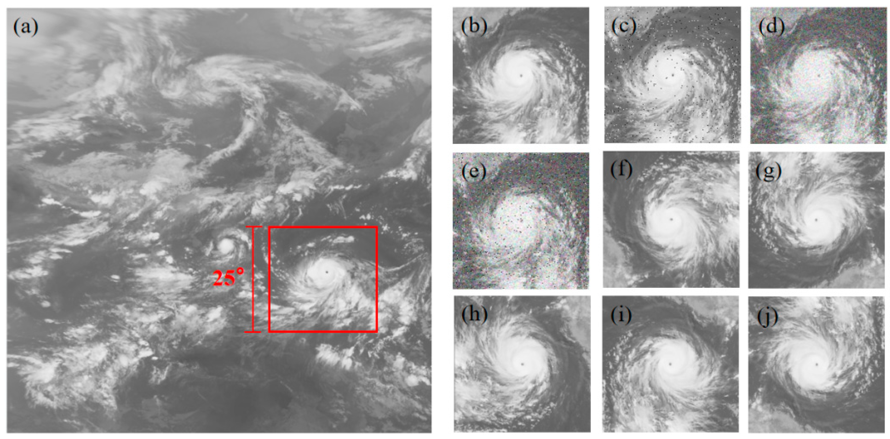
Remotesensing 15 04188 g001
Figure 2. Image transformation: (a) original image; (b) cut-out images; (c) adding salt and pepper noise; (d) adding Gaussian noise; (e) adding salt and pepper and Gaussian noise; (f,g,h) rotating 90°, 180°, 270° anticlockwise; (i) horizontal flip; (j) vertical flip.
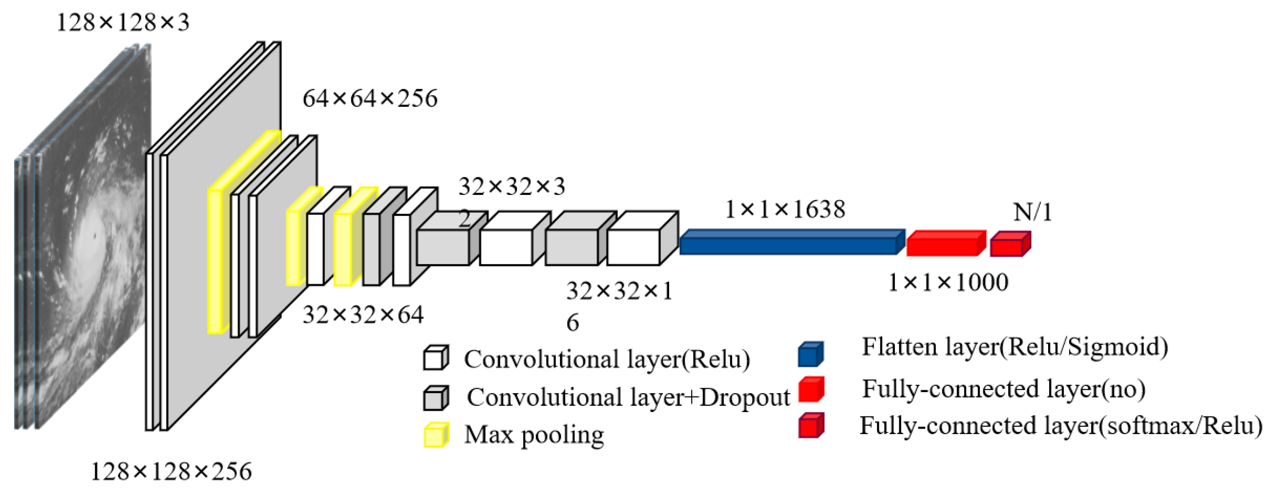
Remotesensing 15 04188 g002
Figure 3. Structures of the DCNN network.
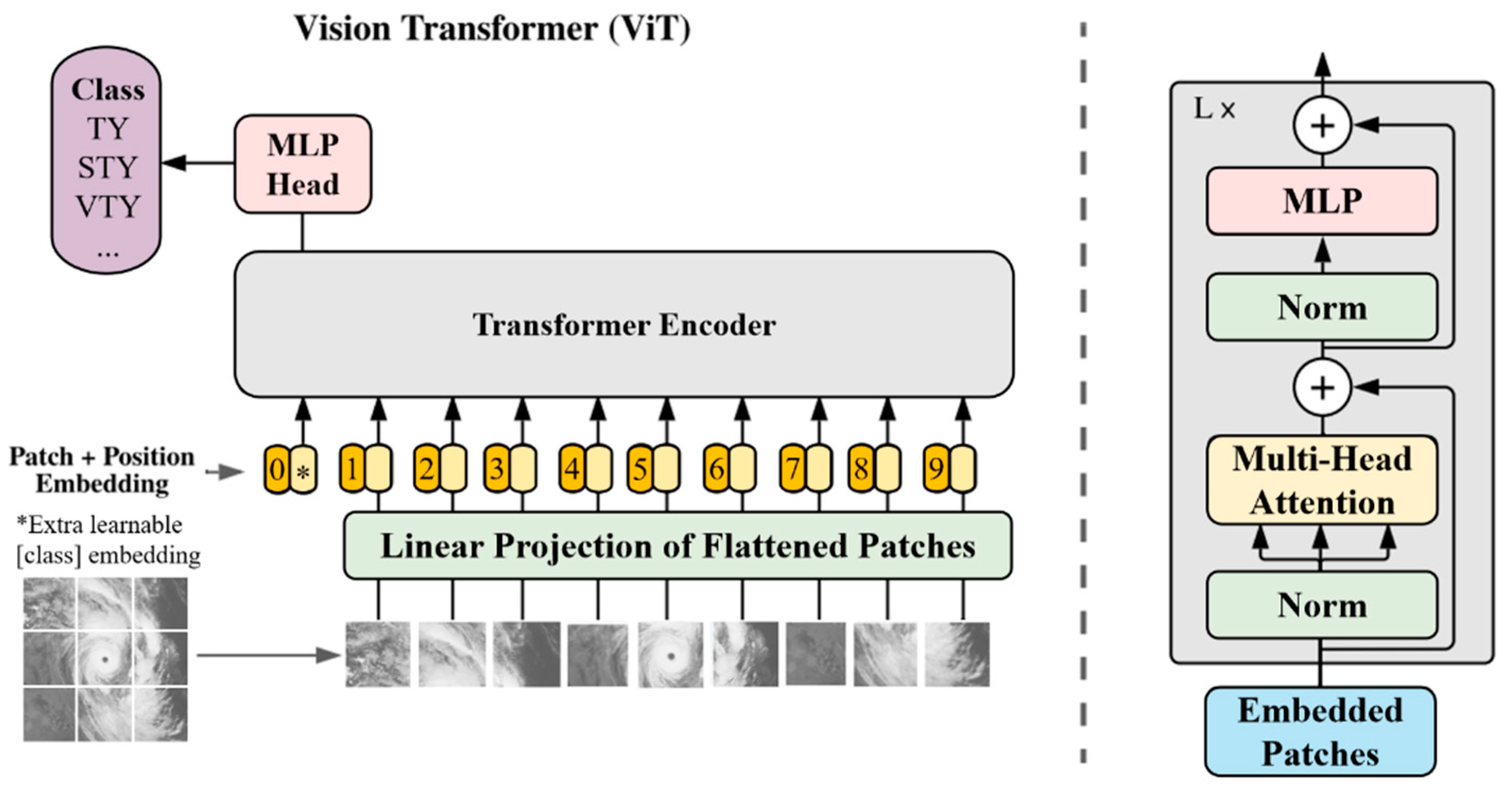
Remotesensing 15 04188 g003
Figure 4. Analysis of the overall structure of ViT.
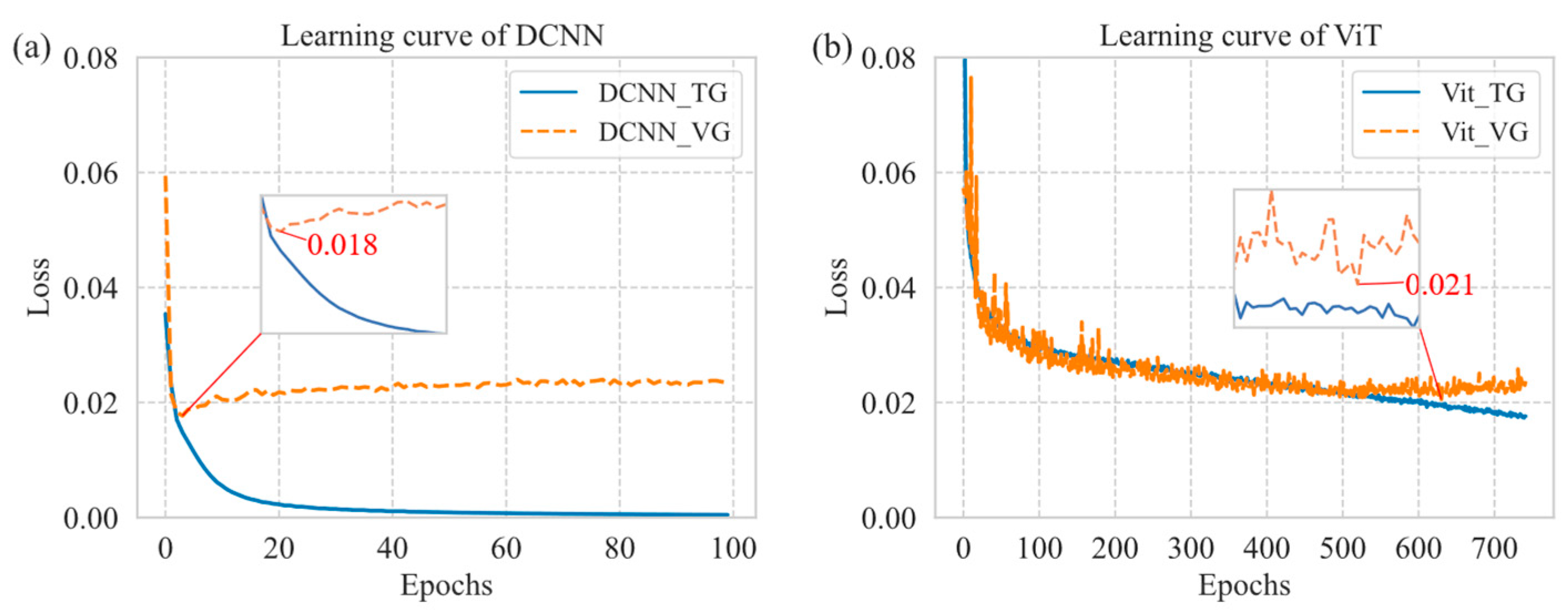
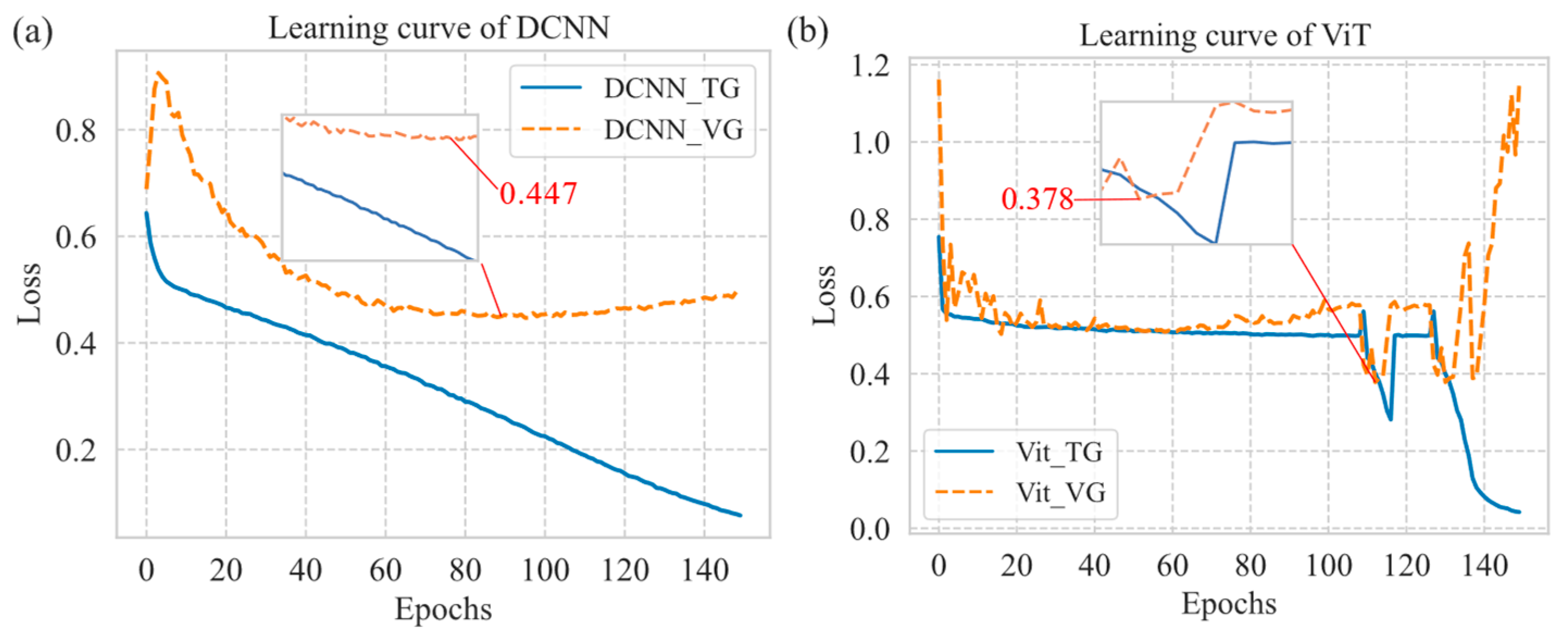
Remotesensing 15 04188 g004
Figure 5. TC intensity regression model learning curves: (a) DCNN; (b) ViT.
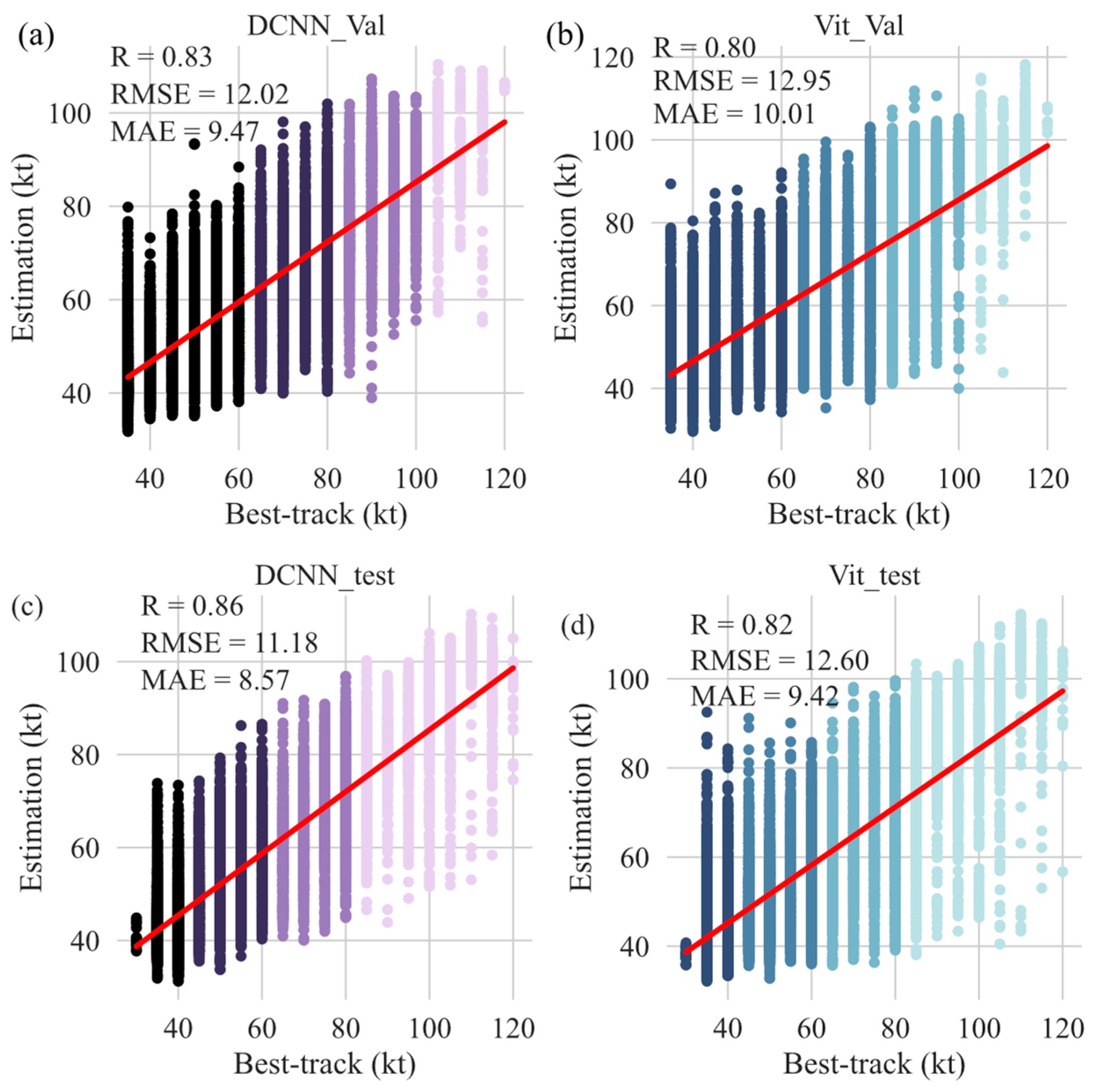
Remotesensing 15 04188 g005
Figure 6. Estimations from validating (Val) and testing (test) processes of DCNN and ViT for the one-stage strategy, compared with best-track data. Red line denotes linear fit of estimation in function of best-track data: (a) DCNN validation, (b) ViT validation, (c) DCNN testing, and (d) ViT testing.
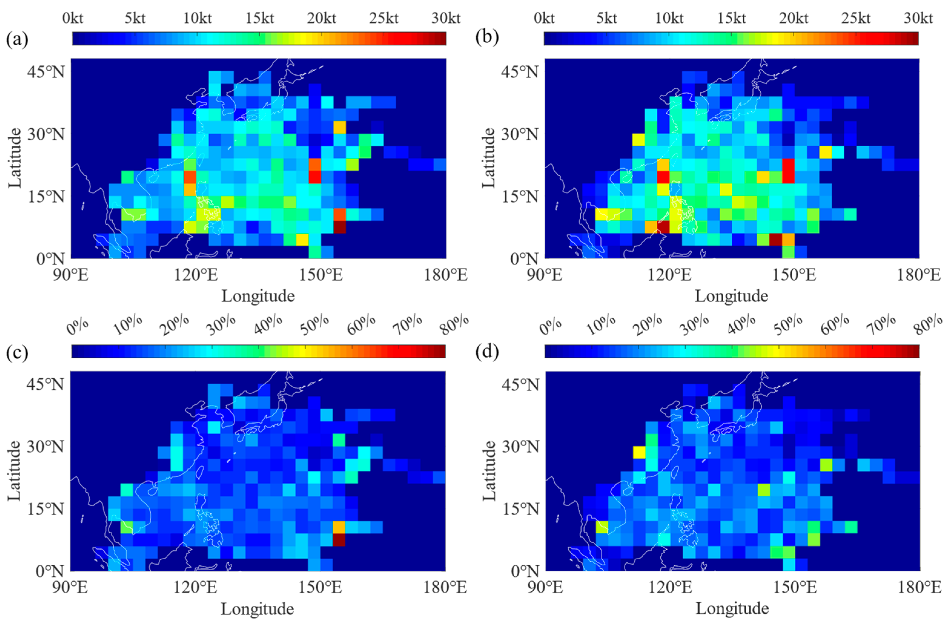
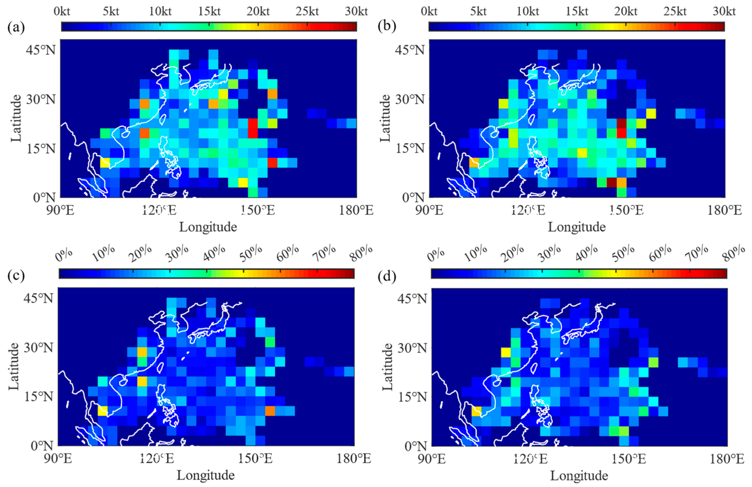
Remotesensing 15 04188 g006
Figure 7. Geographic distribution of estimation errors for DCNN and ViT from one-state strategy: (a) RMSE for DCNN, (b) RMSE for ViT, (c) MAPE for DCNN, and (d) MAPE for ViT.
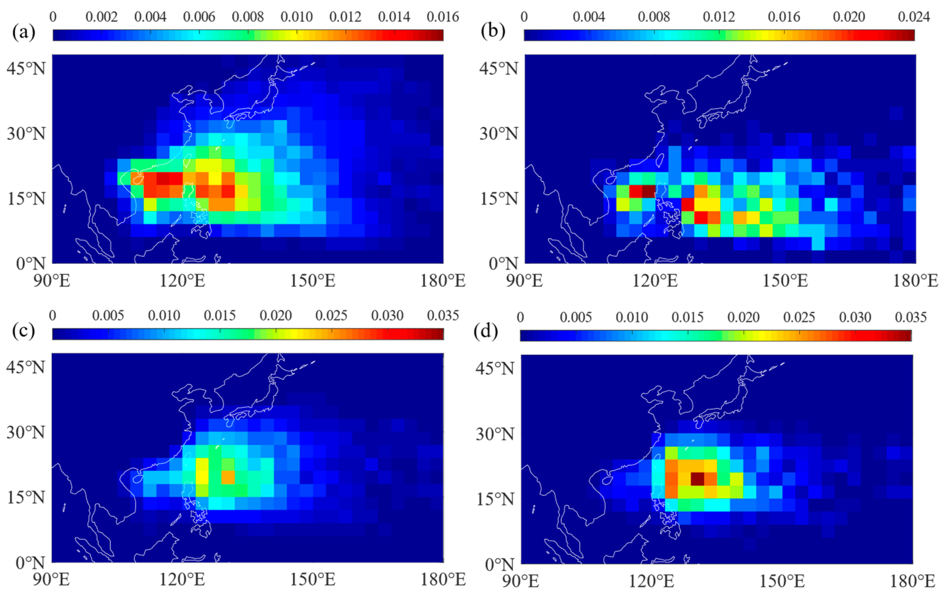
Remotesensing 15 04188 g007
Figure 8. Geographic distribution of appearance probability of: (a) TCs, (b) TC genesis, (c) TCs with MSW > 65 kt, and (d) TCs with MSW > 80 kt.
Remotesensing 15 04188 g008
Figure 9. Learning curves of classification models: (a) DCNN; (b) ViT.
Remotesensing 15 04188 g009
Figure 10. Boxplots of estimation bias for different models via two-stage strategies: (a) DCNN_DCNN, (b) DCNN_Vit, (c) ViT_ViT, and (d)ViT_DCNN.
Remotesensing 15 04188 g010
Figure 11. Geographic distribution of estimation errors from two two-state strategies: (a) RMSE for ViT_DCNN, (b) RMSE for ViT_ViT, (c) MAPE for ViT_DCNN, and (d) MAPE for ViT_ViT.
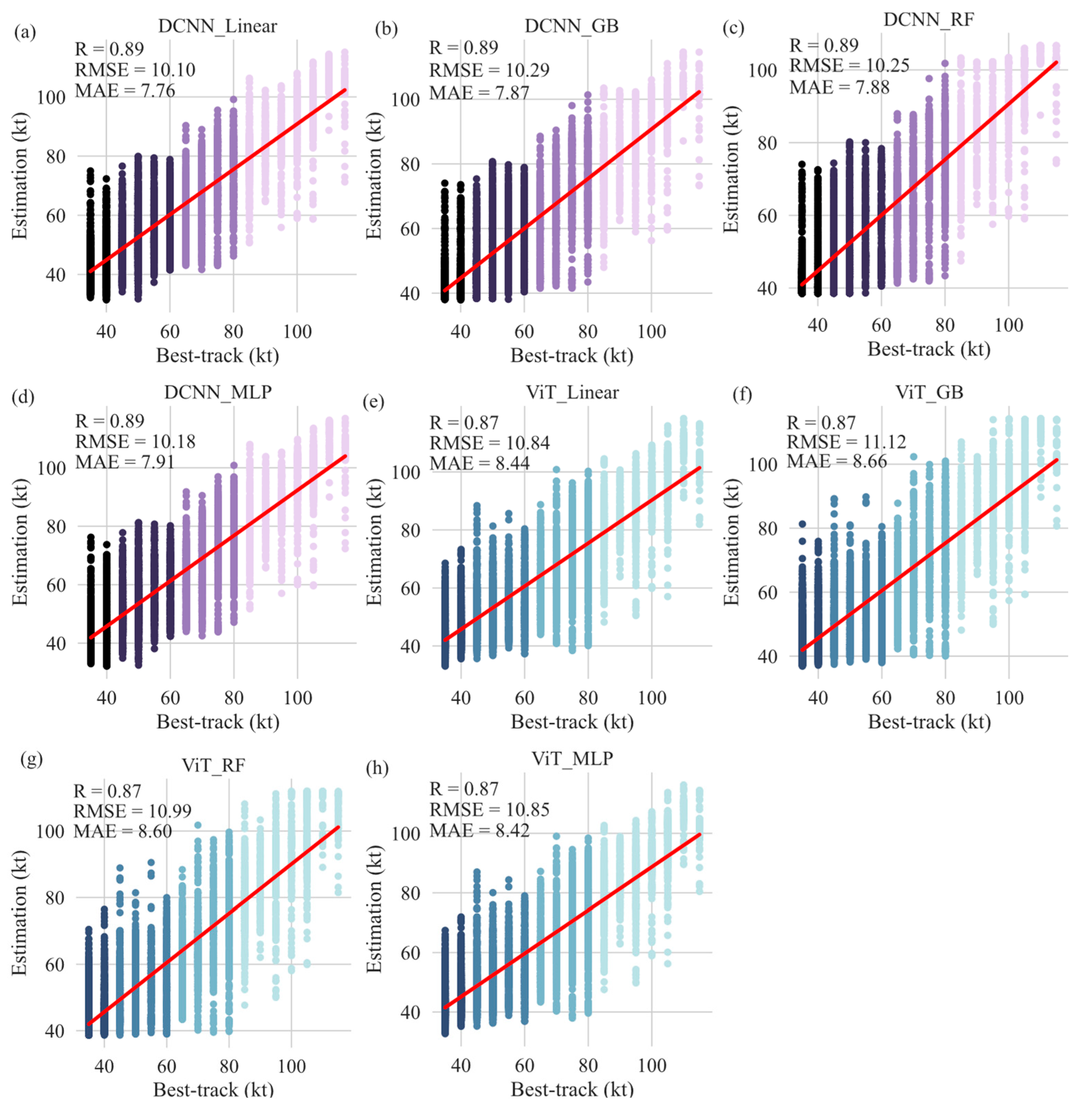
Remotesensing 15 04188 g011
Figure 12. Smoothed estimations from testing process of DCNN and ViT for the one-stage strategy via different smoothing methods: (a,e) using linear weighting; (b,f) using GB; (c,g) using RF; (d,h) using MLP, compared with best-track data.
Remotesensing 15 04188 g012
Figure 13. Geographic distribution of smoothed estimation errors for DCNN_Linear and ViT_MLP from one-state strategy: (a) RMSE for DCNN_Linear, (b) RMSE for ViT_MLP, (c) MAPE for DCNN_Linear, and (d) MAPE for ViT_MLP.
Remotesensing 15 04188 g013
Figure 14. Geographic distribution of smoothed estimation errors for V_D_Linear and V_D_MLP from two-state strategy: (a) RMSE for V_D_Linear, (b) RMSE for V_D_MLP, (c) MAPE for V_D_Linear, and (d) MAPE for V_D_MLP.
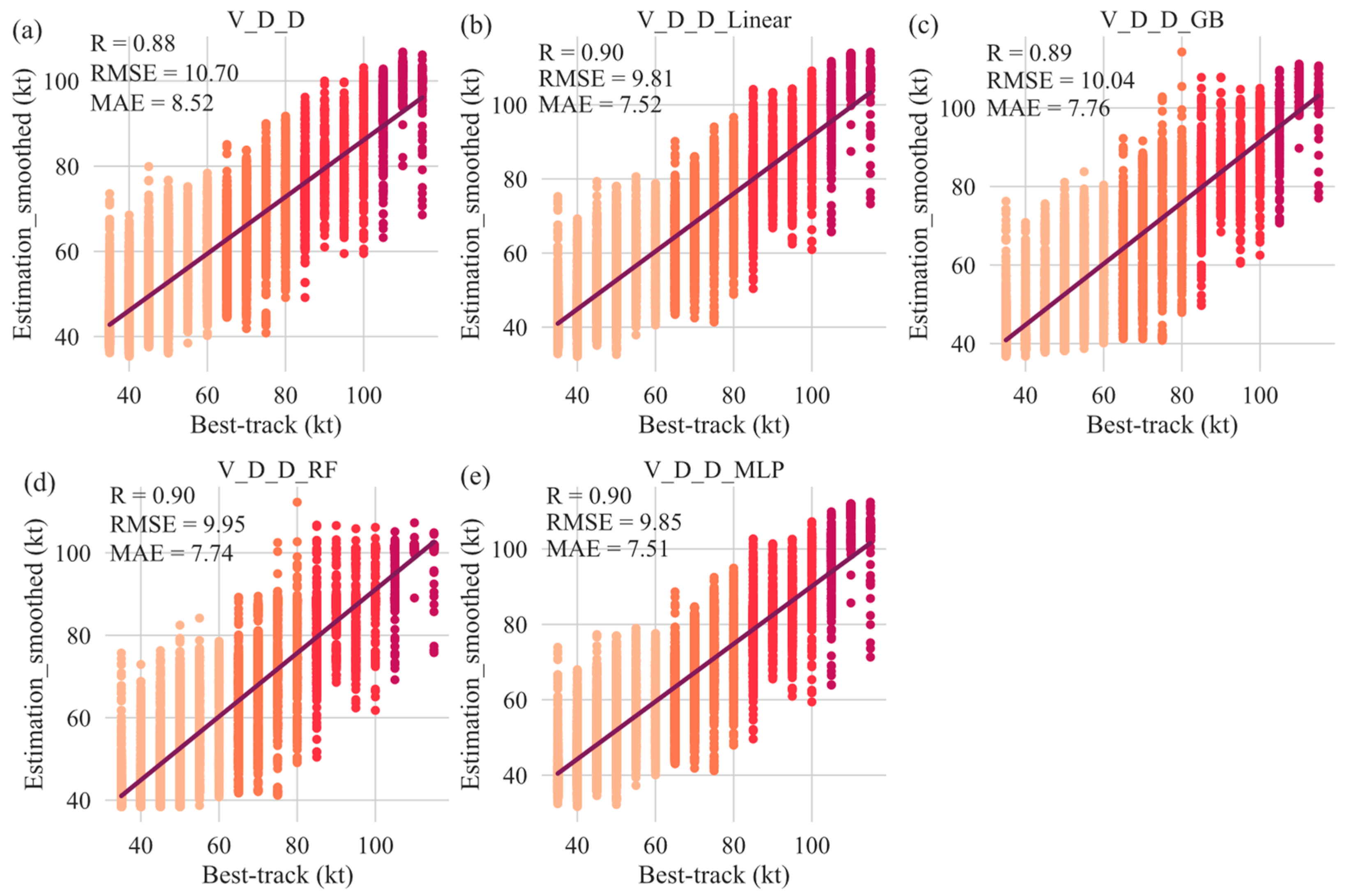
Remotesensing 15 04188 g014
Figure 15. Smoothed estimations from testing process of hybrid strategy models, compared with best-track data: (a) V_D_D, (b) V_D_D_Linear, (c) V_D_D_GB, (d) V_D_D_RF, and (e) V_D_D_MLP.
Remotesensing 15 04188 g015
Figure 16. Geographic distribution of smoothed estimation errors for V_D_D_Linear and V_D_D_MLP from one-state strategy: (a) RMSE for V_D_D_Linear, (b) RMSE for V_D_D_MLP, (c) MAPE for V_D_D_Linear, and (d) MAPE for V_D_D_MLP.
Remotesensing 15 04188 g016
Figure 17. Histogram of errors obtained via different techniques: (a) RMSE, (b) MAE, (c) MAPE, and (d) R coefficient.
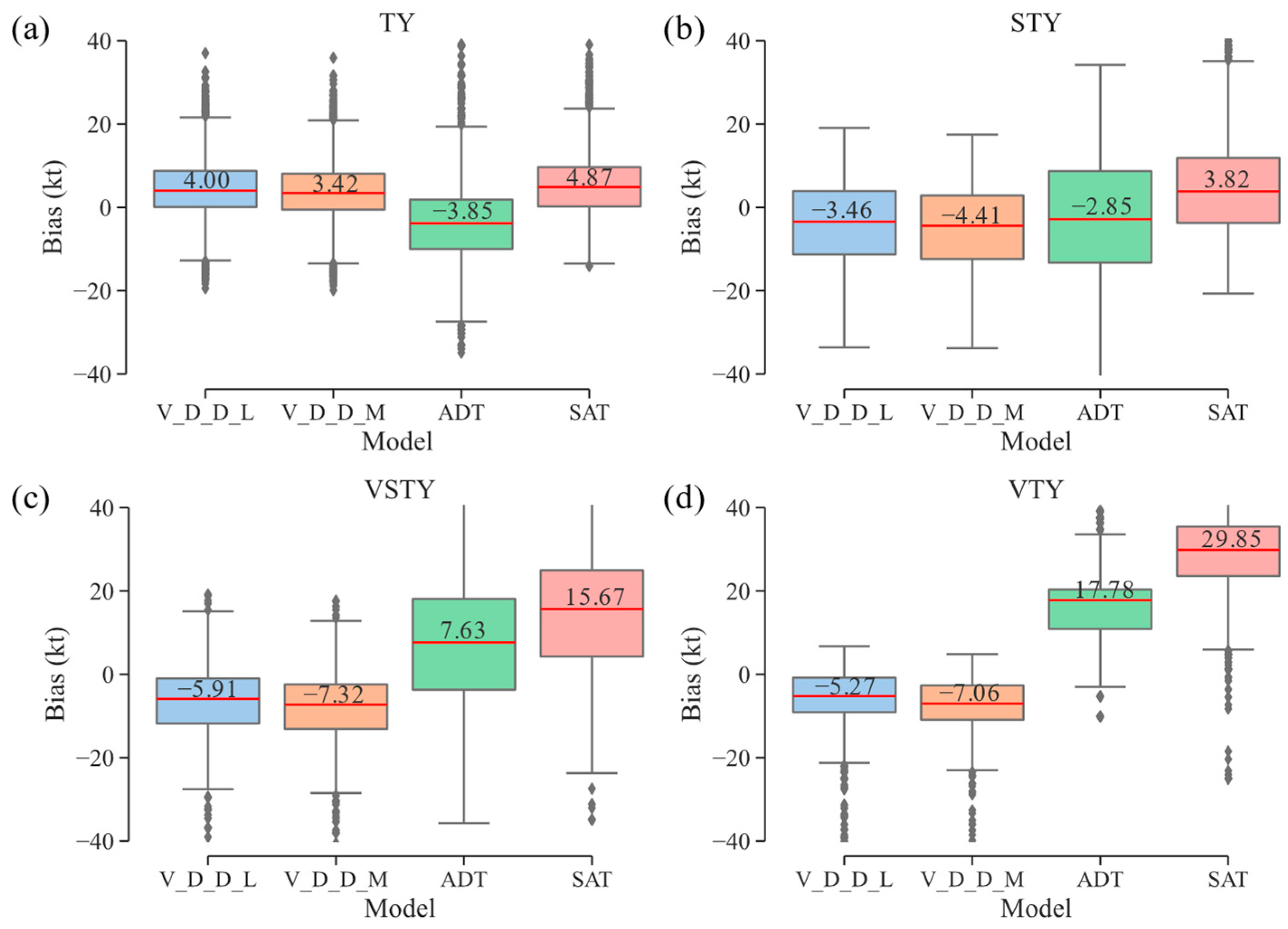
Remotesensing 15 04188 g017
Figure 18. Boxplots of estimation bias for different techniques: (a) for TY intensity samples, (b) for STY intensity samples, (c) for VSTY intensity samples, and (d) for VTY intensity samples.
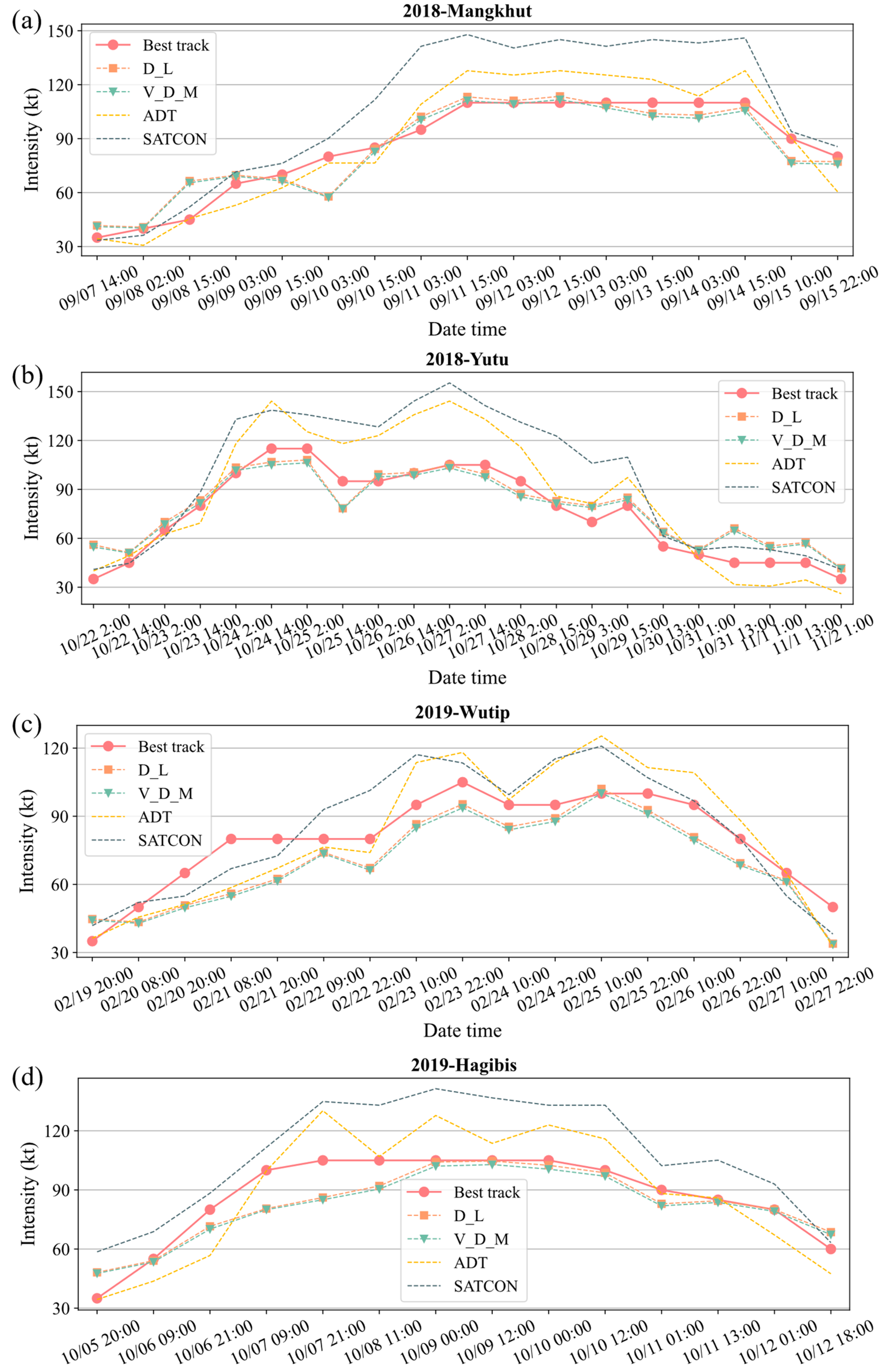
Remotesensing 15 04188 g018
Figure 19. Comparison of estimations via varied methods for four TCs: (a) Mangkhut in 2018, (b) Yutu in 2018, (c) Wutip in 2019, and (d) Hagibis in 2019.
Remotesensing 15 04188 g019
Figure 20. Estimation errors for 4 TCs at varied developing stages (A, B, C represent the formation, mature, and dissipation stage): (a) Mangkhut in 2018; (b) Yutu in 2018; (c) Wutip in 2019; (d) Hagibis in 2019.
Remotesensing 15 04188 g020
Table 1. The number of samples.
YearsTCsSCI Samples
Train2000–2013330158,260
Validation2014–201711352,032
Test2018–202110311,920
Table 2. Confusion matrix of parameters for calculating PRF values.
Confusion MatrixPredicted
PositiveNegative
ActualPositiveNTPNFN
NegativeNFPNTN
Table 3. Performance of regression model during testing process.
ModelDatasetRMSEMAEMAPER
DCNNValidation12.029.470.160.83
Testing11.188.570.160.86
ViTValidation12.9510.010.180.80
Testing12.609.420.170.82
Table 4. Overall performance of the DCNN and ViT classification models.
ModelCategoryValidation AccuracyTesting AccuracyPrecisionRecall RatioF1-Score
DCNNTY0.8050.8340.8750.8640.870
STYS0.7620.7800.771
ViTTY0.8310.8540.8850.8870.886
STYS0.7970.7950.796
Table 5. Confusion matrix of predictions from the DCNN classification model.
DCNNTrue Label
TYSTYSSum
STYVSTYVTY
Predicted labelTY6600768150227540
STYS1041148613265274380
Sum76412254147654911920
Table 6. Confusion matrix of predictions from the ViT classification model.
ViTTrue Label
TYSTYSSum
STYVSTYVTY
Predicted labelTY6775729130177651
STYS866152513465324269
Sum76412254147654911920
Table 7. Performance of four scenarios for the two-stage strategy.
ScenarioRMSEMAEMAPER
DCNN_DCNN12.829.370.170.81
DCNN_ViT13.4510.000.180.79
ViT_ViT12.709.630.170.82
ViT_DCNN11.788.880.160.84
Table 8. Overall performance of the two-state strategy smoothed models.
ModelRMSE (kt)MAE (kt)MAPER
D_D_Linear12.079.160.160.84
D_D_GB12.059.170.160.84
D_D_RF12.009.150.160.84
D_D_MLP12.139.150.160.84
V_D_Linear10.648.100.150.88
V_D_GB10.908.290.150.87
V_D_RF10.858.300.150.87
V_D_MLP10.658.090.150.88
Table 9. Comparison of the best estimation performance in this study with those in references.
ModelRMSE (kt)MAE (kt)TC YearReference
ADT9.011.248.672018Olander et al. [4]
DAV-T14.3-2007–2011Ritchie et al. [37]
SATCON8.97.702008–2010Velden and Herndon [12]
TCIENet10.127.942017Zhang and Liu [25]
CNN-TC12.25-2015–2016Chen et al. [23]
VGG1913.23-2015–2016Combinido et al. [21]
CNN 110.19-2015–2018Wang et al. [24]
V_D_D_Linear9.817.522018–2019This study
V_D_D_MLP9.857.51
1 dataset is split randomly in the given proportion.
Disclaimer/Publisher’s Note: The statements, opinions and data contained in all publications are solely those of the individual author(s) and contributor(s) and not of MDPI and/or the editor(s). MDPI and/or the editor(s) disclaim responsibility for any injury to people or property resulting from any ideas, methods, instructions or products referred to in the content.

