1. Introduction
In the field of remote sensing, hyperspectral imaging, and multispectral imaging systems occupy an important position. Hyperspectral imaging has been widely used in mineral detection, environmental detection [
1], climate monitoring [
2], and classification [
3]. Hyperspectral images are obtained by hyperspectral sensors capturing sunlight reflected from an object or scene. During the acquisition of the image, it is affected by the light, resulting in a reduced spatial resolution of the image [
4], but with rich spectral information. In contrast, multispectral images have only a few bands, but the images are rich in spatial information. In the past two decades, a lot of efforts have been made to obtain hyperspectral images with high spatial resolution, and image fusion is the most economical, applicable, and effective means among all methods. The fusion mainly extracts effective high spatial resolution information from source images such as multispectral images and panchromatic images (PAN) and incorporates it into hyperspectral images. Fusion into hyperspectral images to obtain hyperspectral images with high spatial resolution helps to accurately identify observation scenes with high spatial resolution, etc. The most common fusion method is to obtain high spatial resolution hyperspectral images (HRHS) by fusing high spatial resolution multispectral images (HR-MSI) and low spatial resolution hyperspectral images (LR-HSI). At the same time, when an image is reduced in size, the redistribution of pixel information and interpolation algorithms results in a loss of detail or distortion of the original image, a process known as the “scaling effect”. Conversely, when a low-resolution image is scaled up to a higher resolution, this is often accompanied by a loss of information, and the image may appear blurred, distorted, or show unrealistic details, a process known as the “counter-scaling effect”.
In the early studies of fusion algorithms, sharpening methods were mainly used to fuse PANs and MSIs possess high spatial resolutions [
5]. In 2019, Meng et al. [
6] reviewed the development history of pansharpening and divided it into two main categories: component replacement (CS) [
7,
8] and multi-resolution analysis (MRA) [
9,
10,
11], among which the more famous methods are based on hue–intensity–saturation (HIS) [
12], wavelet-based techniques [
13,
14], principal component analysis (PCA) [
15], the Laplace pyramid [
16], etc. Yokoya et al. [
17] found that sharpening fusion methods does not improve the spatial resolution of each spectral band very well after conducting extensive experiments. There is also a growing interest in the study of multispectral and hyperspectral image fusion (MHF) algorithms. A method often referred to as the multi-sharpening process involves the most popular techniques, including matrix factorization [
18,
19,
20,
21,
22,
23,
24] and tensor decomposition [
25,
26,
27,
28,
29,
30,
31,
32]. In addition, some new research results have appeared in recent years. For example, in 2020, Feng et al. [
33] proposed a two-by-two matching based on a spatial–spectral graphical regularization operator for the hyperspectral band selection method, which encodes its geometric structure by constructing a spatial–spectral information map using spatial–spectral adjacencies. In 2021, Huang et al. [
34] proposed a subspace clustering algorithm for hyperspectral images, which improves the model’s noise immunity by introducing an adaptive spatial regularization method. In 2022, Qin et al. [
35] proposed a multi-focus image fusion method based on sparse representation (DWT-SR) by decomposing multiple frequency bands and shortening the algorithm’s running time by utilizing GPU parallel computing, which features high contrast and richer spatial details. In 2022, Zhang et al. [
36] proposed a sparse demixing method in order to avoid inaccuracy in extracting the endmember information and to retain the original domain super-pixel inter-correlation and spectral variability in the approximated image domain. In 2023, Y et al. [
37] designed a new attentional reinforcement learning network to accomplish the spatio-temporal prediction of wind power.
The matrix-based decomposition method is widely used in MHF problems because of its clear motivation and excellent performance. After matrix decomposition, the potential factors have a strong physical meaning, such as endmember and abundance are non-negative [
22,
38,
39]. In 2011, Yokoya et al. [
18] used a coupled non-negative matrix decomposition (CNMF) unmixing method to decompose hyperspectral and multispectral data into endmember matrices and abundance matrices alternatively; the cost function in the model is non-convex, resulting in an unsatisfactory algorithm fusion. In the same year, Kawakami et al. [
40] decomposed the target image HRHS into a basis matrix and a sparse matrix and then recombined the spectral basis matrix of LR-HSIs and the coefficient matrix of HR-MSIs to obtain them. In 2014, Simoes et al. [
21] introduced total variation (TV) regularization in a subspace-based HRHS fusion framework, which effectively eliminated the noise. In 2015, Lanaras et al. [
41] completed the acquisition of HRHSs by jointly unmixing two input images into a pure reflection spectral matrix and a mixed sparse matrix. In 2018, Kahraman et al. [
42] proposed a graph regularization
-sparse constrained non-negative matrix decomposition-based image fusion method that enhances the fusion performance by using the
and streamwise regularization to enhance the unmixing. In 2021, Mu et al. [
43] introduced a spectral-constrained regularization term to avoid spectral distortion and maintain spectral integrity based on the coupled non-negative matrix decomposition (CNMF) algorithm. In 2022, Khader et al. [
44] proposed a new non-negative matrix factorization decomposition-inspired deep unfolding network (NMF-DuNet) to fuse LR-HSIs and HR-MSIs using a non-negative coefficient matrix and orthogonal transformation coefficient constraints. In 2022, Han et al. [
45] proposed a fusion model based on spatial nonlocal similarity and low-rank prior learning to solve the problem of the existing methods that cannot simultaneously consider the spatial and spectral domain structure of hyperspectral image cubes; however, there problems still exist, such as the partial loss of spectral correlation, and the complexity of the algorithm is high. In 2023, Lin et al. [
46] proposed a highly interpretable deep HSI-MSI fusion method based on a 2D image CNN-based Gaussian denoiser, which can fuse the LR-HSIs and HR-MSIs under a known imaging system and achieve good fusion performance.
While there are many other improved algorithms based on matrix decomposition, they all require the conversion of 3D data into a 2D data format, resulting in difficult exploitation of the spatial–spectral correlation in LR-HSIs. In contrast, the fusion method based on tensor decomposition can effectively avoid such defects and becomes a new research hotspot for the MHF problem. It regards LR-HSIs and HR-MSIs as a 3D data cube consisting of two spatial dimensions and one spectral dimension (i.e., spatial × spatial × spectral), where the spectral dimension is the key to identifying objects in the scene. Based on this fact, in 2018, Kanatsoulis et al. [
47] proposed a coupled tensor decomposition-based (CTD) framework to solve the MHF problem, and, using canonical polyadic decomposition (CPD) uniqueness, they proved that HRHSs can be recovered under mild conditions. Xu et al. [
48] constructed the nonlocally similar patch tensor of LR-HSIs based on HR-MSIs, calculated the smoothing order of all patches used for clustering, preserved the relationship between HRHSs and HR-MSIs by CPD, and proposed a multispectral and hyperspectral fusion algorithm based on the CPD decomposition of the nonlocally coupled tensor. In 2020, Prévost et al. [
25] extended a similar idea to the Tucker decomposition for solving MHF problems with better results. In the same year, Xu et al. [
27] proposed a one-way TV-based fusion method, which decomposes the HRHS into a core tensor and three modal dictionary forms, and imposes the
-norm and the one-way TV characterizing sparsity and piecewise smoothness, respectively. In 2021, Peng et al. [
49] introduced a global gradient sparse nonlocal low-rank tensor decomposition model to characterize the nonlocal and global properties of HRHSs, which can effectively capture the spatial and spectral similarity of the nonlocal cube, and introduced spatial–spectral total variation (SSTV) regularization to reconstruct HRHSs on the nonlocal domain low-rank cube, thus obtaining global spatial piecewise smoothness and spectral consistency. In 2022, Prévos et al. [
50] proposed a fast coupling method based on the Tucker approximation into this work to take full advantage of the coupling information contained in hyperspectral and multispectral images of the same scene. After a large number of experiments, CPD and Tucker have been proven to have excellent recoverability on the MHF problem, and the frameworks of both have shown excellent performance; however, the failure to utilize the physical interpretation of the potential factors makes it difficult for both to utilize the a priori information to improve the algorithmic fusion effect. In addition, a new tensor decomposition, called tensor ring (TR) decomposition, is proposed in [
51], which decomposes higher-rank tensors into cyclically contracted third-rank tensor sequences. This method inherits the representation capability of CPD and extends the low-rank exploration capability of Tucker decomposition. In 2022, Chen et al. [
52] proposed a factorially smoothed TR decomposition model, which solved the problem that the spatial–spectral continuity of HRHSs could not be preserved in the existing TR decomposition model; however, the algorithm has high requirements on hardware equipment in the case of a large amount of spectral data. In summary, CPD and Tucker decomposition are not necessarily better than the methods for low-rank matrix estimation, and TR decomposition is not necessarily the best choice.
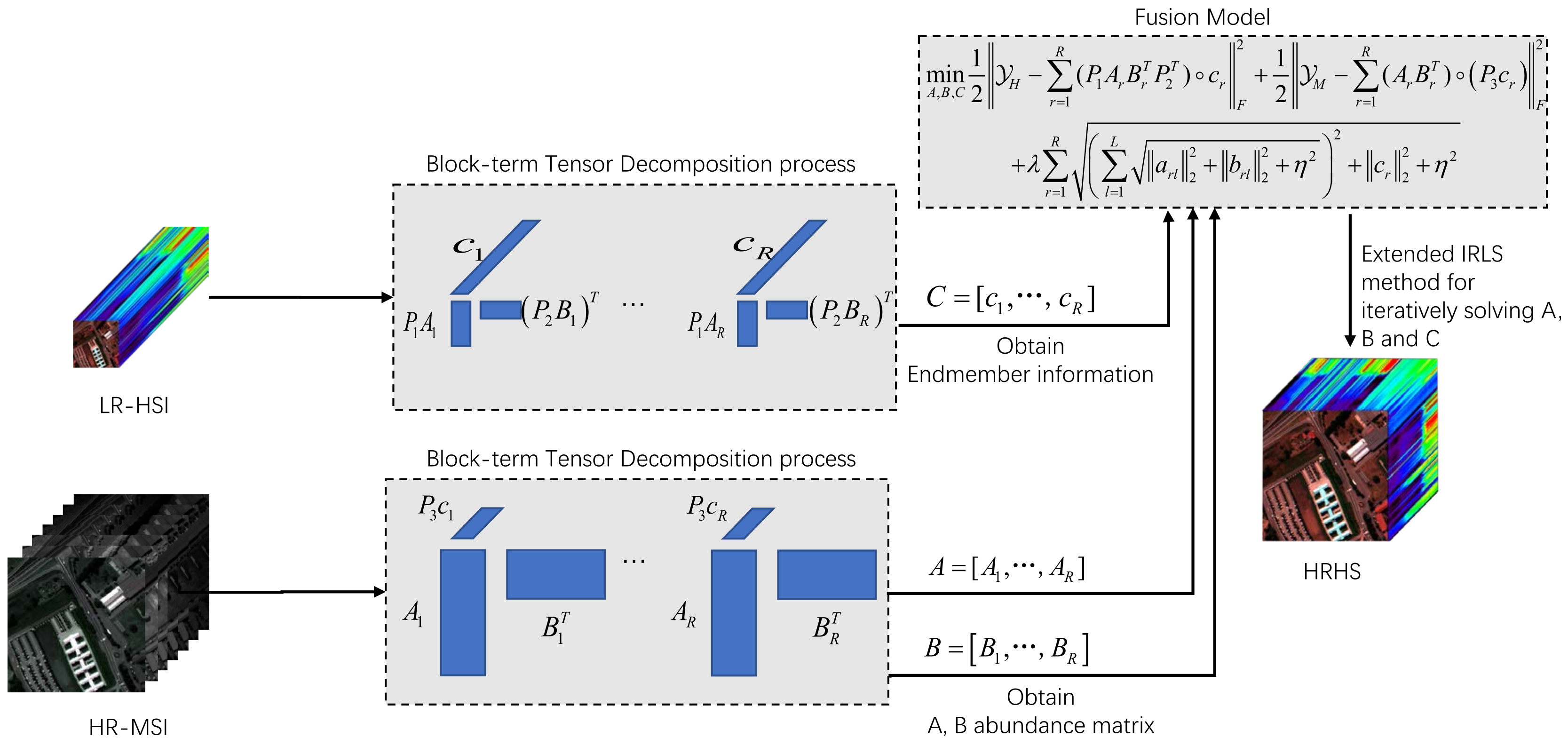
In contrast, linear mixed models (LMM) using matrixed LR-HSI and HR-MSI low-rank structures can circumvent such problems, and their endmembers and abundances possess a strong physical interpretation, which can be further improved by imposing structured constraints or regularization on them, especially in the presence of noise, where this information is particularly important. In 2018, Li et al. [
32] demonstrated, under a relatively restricted condition, that the coupled matrix decomposition model is able to identify recovered HRHSs. For example, if the abundance matrix of an HR-MSI is sparse, i.e., under tensor notation, the LMM can be rewritten to approximate the 3D spectral data as the sum of the outer products of the endmembers (vectors) and the abundance maps (matrices). This approach can fully match the matrix-vector third-order tensor decomposition, which decomposes the tensor into the sum of the component tensors, each of which in turn consists of matrix-vector outer products [
53]. The matrix-vector third-order tensor factorization can also be regarded as the block-term tensor decomposition (BTD). Therefore, matrices and vectors in the BTD can be used as abundance maps and vectors, respectively, with non-negativity and coupling properties. In 2019, Zhang et al. [
54] proposed a coupled non-negative BTD model [
55,
56,
57]. The BTD was used to decompose the spectral images to take full advantage of the physical significance of their potential factors, but the use of regularization to improve the algorithm’s performance and application in multiple scenarios was not considered. In 2021, Ding et al. [
58] reformulated the recovery HRHS process as a special block-term tensor model, imposing constraints and regularization to improve the performance of the algorithm, but failed to take into account the effects between individual abundance matrices, and there were limitations in the experimental scenario. In 2022, Guo et al. [
59] proposed a coupled non-negative block-term tensor decomposition algorithm based on regularization. Consider the sparsity and smoothness of the individual abundance and the endmember matrix; to these, add the
-norm and bidirectional TV. However, the
-norm has a non-smoothness property and is not the best choice for the regularizer. The algorithm takes too long to run. Therefore, a joint-structured sparse block-term tensor decomposition model (JSSLL1) based on joint-structured sparsity is proposed by introducing the
-norm to promote the structured sparsity of the block matrix composed of potential factors and eliminate the scaling effects present in the model, The
-norm is introduced to the endmember to counteract the counter-scaling effects in the decomposition model. Finally, the block matrix and endmember are coupled together, and the
-norm is imposed on them to promote the elimination of the block matrix. The contributions of the proposed algorithm are as follows.
During the reconstruction of an HRHS, in order to promote the sparsity of the abundance matrix and counteract the scaling effect existing in the abundance matrix during image recovery, the two abundance matrices are superimposed to obtain the chunk matrix, and the blending parametrization -norm is added to it.
In the process of reconstructing an HRHS, the counter-scaling effect of the endmember vector is considered and avoided by adding the -norm to the endmember vector.
In the block-term tensor factorization model, the accuracy of the rank is a key factor that is unknown a priori. Inaccurate rank estimation may cause noise or artifacts to interfere with the experimental results. In order to solve this problem, this paper introduces the reweighted coupling of the block matrix and the endmember matrix and introduces the mixing norm. Through this method, the influence of the inaccuracy of the rank estimation can be reduced while maintaining flexibility, so as to improve the reliability of the experimental results.
Below is the remainder of this article.
Section 2 describes the background and related works.
Section 3 describes the MHF method and optimization scheme based on the joint-structured sparse LL1 model.
Section 4 describes the experimental setup, visualization of experimental results, evaluation metrics, and classification results and develops the discussion.
Section 5 summarizes the algorithm proposed in this paper and future improvement directions.
2. Background
Because LR-HSIs possess two spatial dimensions and one spectral dimension, they can be regarded as third-order tensors. In recent years, with the continuous improvement of the MHF algorithm, the tensor decomposition method has been widely used because of its ability to avoid an excessive loss of spatial and spectral information. The two more common models are the CPD and Tucker models.
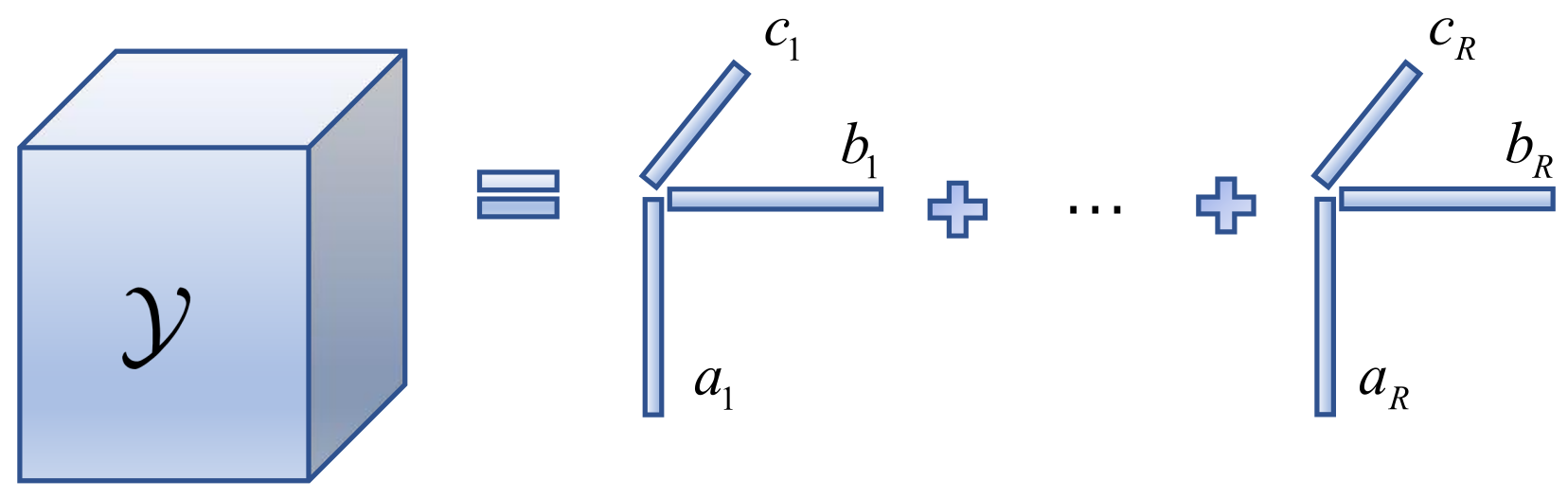
The CPD model [
60] is a tensor rank decomposition model. The procedure is shown below, which allows the decomposing of the tensor into the total of multiple tensors of rank one. The mathematical model is as follows (note: see
Appendix A for an explanation of the relevant symbols in the text).
where
,
, and
are second-order factor matrices;
is a third-order tensor.
Figure 1 represents the flow of CPD.
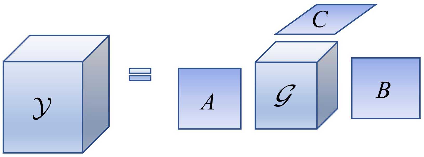
The Tucker model [
61] is also widely used in the field of imaging, and it is a higher-order form of principal component analysis (PCA), which focuses on decomposing the tensor into a core tensor and three-factor matrices. The Tucker decomposition process is shown in
Figure 2. The mathematical model is expressed as [
62]:
where
,
, and
are the factor matrices;
is a third-order core tensor.
In addition to the two tensor models mentioned above, the BTD model is gradually being applied to the field of image fusion because the potential factors have a good physical interpretation, such as in the work performed previously [
59]. In solving the MHF problem, compared with the CPD and Tucker models, potential factors in the BTD model, respectively, represent the abundance and the endmember, which have a physical sense of non-negativity and spatial smoothness, and contribute to the utilization of various prior knowledge in the image fusion process.
By combining the advantages of the CPD and Tucker models, the BTD of
(abbreviation: LMN model) in general form can be expressed as:
where
,
,
, and
. The LMN decomposition process is shown in
Figure 3. The above description shows that the BTD is approximating the tensor
by
R component tensors, and each tensor is a Tucker of
. If each component tensor rank is one, it can be treated as a CPD. Similarly, if
, then Equation (
3) is the Tucker model of
. In other words, the BTD can decompose a tensor into the sum of multiple component tensors, and this process can be viewed as the CPD, while each component tensor decomposition is viewed as a Tucker decomposition. This overcomes the problem that each component tensor rank must be one in the CPD and lifts the restriction that the Tucker decomposition has only one component tensor. It is a combination of the CPD and the Tucker decomposition.
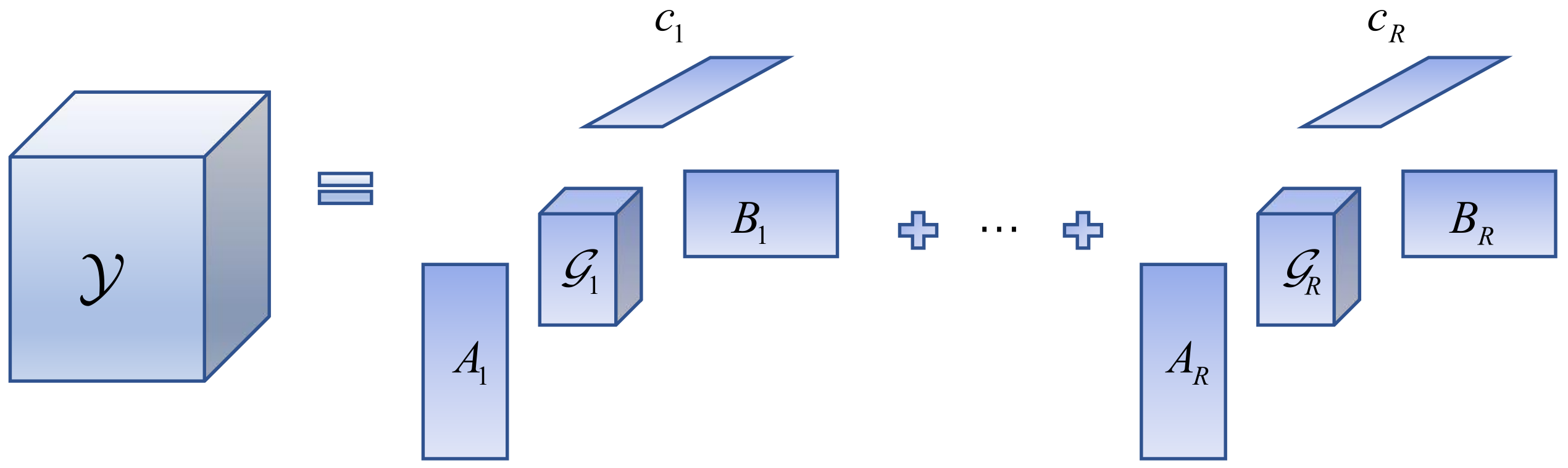
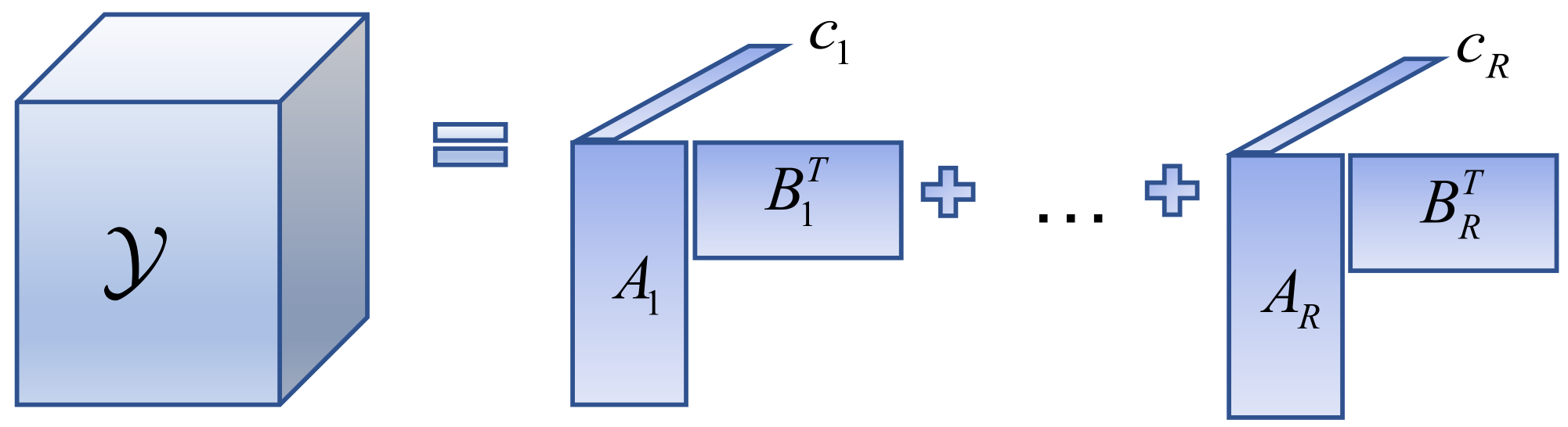
Usually, the special BTD model is adopted to resolve the MHF problem. The special BTD model of
(abbreviation: LL1 model) is obtained when each member tensor degenerates to an
matrix, and each
takes the same value. The decomposition process of the LL1 model is shown in
Figure 4. The mathematical model is as follows:
where
,
, and
. Among these,
and
are, respectively, the subblocks of the block matrices
A and
B, denoted as
,
. In general, the full column rank requirement for
and
is
. Under mild conditions, the LL1 model possesses a nice property, i.e.,
and
are identifiable until the alignment and scaling ambiguities arise, which is induced as follows (Theorem 4.7 of [
56]). The potential factors
and
represent the abundance information; the former represents the abundance information of the endmember
r, and the latter represents the
rth endmember.
In summary, the CPD and Tucker models are both low-rank models (see
Figure 1 and
Figure 2), capable of “encoding” dependencies in different dimensions of the data and often used in spectral image modeling with good recoverability [
25,
47]. Although this is useful for recovering an HRHS, it is not necessarily better than the BTD-based MHF approach in practice. The BTD-based MHF framework can be used to introduce the structural information of potential factors using their physical interpretation, which helps to standardize the MHF criteria with a priori knowledge.
4. Experiments and Analysis
4.1. Datasets
4.1.1. Standard Datasets
The Pavia University dataset [
59] was acquired by the Reflection Optical System Imaging Spectrometer (ROSIS) over the city of Pavia. The size of the acquired image is 610 × 340 and consists of 115 spectral bands with an image resolution of 1.3 m. To enhance the experimental effect, the sub-image located in the upper left corner of the image was selected as the experimental image after removing the band containing water vapor. The size of the experimental image is 256 × 256 × 102, and the image contains rich features such as houses, roads, and trees.
The Indian Pines dataset [
59] was acquired by the Airborne Visible Infrared Spectroscopic Imager (AVIRIS) over Indian, U.S.A. The AVIRIS wavelength range is between 0.4
m and 2.5
m with a spatial resolution of 20 m. After removing 24 bands that cannot be reflected by water, the remaining bands were used for the study. Given the experimental requirements, the final image size selected was 144 × 144 × 200.
4.1.2. Local Dataset
The dataset of Ningxia Sand Lake [
59] was acquired by the WFV4 multispectral imager on the Gaofen-1 (GF1) satellite and the AHSI hyperspectral imager on the Gaofen-5 (GF5) satellite over Ningxia Sand Lake. The WFV4 wavelength range is 0.45–0.89
m, the spatial resolution is 16 m, and the size of the acquired multispectral image is 12,000 × 13,400. The wavelength range of AHSI is 0.4–2.5
m, the spatial resolution is 30 m, it consists of 330 bands, and the size of the acquired hyperspectral image is 2774 × 2554. After removing 187 bands with high noise again, the remaining bands are used as the research object. The experimental images were intercepted at the same position as the acquired multispectral and hyperspectral images, and the final selected image sizes were 254 × 254 × 3 for the HR-MSI and 254 × 254 × 143 for the LR-HSI, respectively.
4.2. Experimental Setup
4.2.1. Experimental Environment
Eight algorithms, CNMF [
18], Hysure [
21], FUSE [
22], SCOTT [
25], IRSR [
45], STEREO [
47], BTD [
54], and SCLL1 [
58], were selected as comparison tests. Among them, SCOTT and STEREO are based on the Tucker and CPD models to solve the MHF problem, respectively; the BTD and SCLL1 are based on the BTD model to solve the MHF problem. Considering the different experimental environments of each algorithm, it is often difficult to achieve the effect in the original literature by directly adopting the parameter settings of the original literature under the current experimental environment, so this paper optimizes the parameters of other algorithms under the current experimental environment. Specifically, standard normally distributed pseudo-random numbers are used as initialization values for all algorithms, and the optimal parameter values are selected through ablation experiments; the hyperspectral decomposition threshold in the CNMF experiments is set to
, the multispectral decomposition threshold is set to
, and the outer recirculation decomposition threshold is set to
. The value of the weighting parameter in STEREO is set to
. The regularization parameter is set to
and
in SCLL1, and the parameters of the other algorithms that are not mentioned in the original text are used to set the parameters. The CPU in the experimental equipment is Intel(R) Xeon(R) Gold 6154; the RAM size is 256G. The operating system is 64-bit Windows 10. The experimental platform is Matlab R2017b.
4.2.2. Degradation Model
The local datasets are acquired using multispectral and hyperspectral sensors in the acquisition process to directly obtain the HR-MSI and LR-HSI, respectively. However, the standard dataset is different in that it is a hyperspectral dataset acquired by a hyperspectral sensor and lacks a corresponding multispectral dataset to perform fusion experiments. Therefore, the standard dataset is generally used as a reference image when fusion experiments are being performed, and the HR-MSI and LR-HSI used in the experiments are obtained from it by degradation, respectively. In this paper, the degradation model follows the literature [
22,
32,
68] and strictly follows the Wald agreement. The process of acquiring the LR-HSI is such that the standard dataset is fuzzed using a 9 × 9 Gaussian kernel and sampled at 4-pixel intervals. The process of acquiring the HR-MSI is referred to in the literature [
47]. At last, noise is added for the LR-HSI and HR-MSI.
4.3. Numerical Evaluation Indicators
In order to evaluate the differences between the algorithms proposed in this paper and the comparison algorithms in further detail, it is necessary to evaluate them with the help of numerical evaluation metrics, in addition to direct observation of the HRHS quality and difference images of each algorithm. In recent years, many evaluation metrics have emerged with the continuous improvement of the algorithms, but metrics such as the peak signal-to-noise ratio (PSNR), structural similarity (SSIM) [
69], correlation coefficient (CC), universal image quality index (UIQI) [
70], root mean squared error (RMSE), Erreur Relative Globale Adimensionnelle de Synthese (ERGAS) [
71], spectral angle mapper (SAM) [
72], and TIME, which appear in the literature [
4,
17], are widely used, and they can comprehensively assess the superiority of the algorithms in terms of spatial information, spectral information, and algorithm efficiency. The specific details of these evaluation metrics are described in detail in our separate work [
59]. Among these, the larger the PSNR value, the better the image quality; the closer the SSIM, CC, and UIQI values are to one, the better the quality of the HRHS fusion; the closer the values of the RMSE, ERGAS, SAM, and TIME are to 0, the better the fusion effect. Detailed definitions follow:
The peak signal-to-noise ratio (
PSNR) evaluates the level of image distortion or noise. The general situation of
PSNR is between 30 dB and 50 dB. In the ideal case, it is expected to be as high as possible, with
∞ representing the optimal value. It should be specifically noted that when the
PSNR is more than 30 dB, it is difficult for the human eye to see the difference between the fused image and the reference image. The definitions are as follows.
The structural similarity (
SSIM) is used to calculate the structural similarity between the HRHS and the reference image in the spatial domain [
69]. The
SSIM ranges from −1 to 1. When the two images are identical, the
SSIM value is equal to one. The definitions are as follows.
The correlation coefficient (
CC) describes the degrees of spectral likeness with respect to the objective image, as well as the fusion image. The
CC is based on a scale from −1 to 1. The closer the
CC is to one, the higher their positive correlation. The definitions are as follows.
The universal image quality index (
UIQI) [
70] is specifically used to detect the average correlation between the reference image and the fused image. If the fused image is closer to the reference image, the
UIQI value is closer to a value of one, which means a better reconstruction effect. The definitions are as follows.
The root mean squared error (
RMSE) is an important index describing the root mean squared error between each band of the reference image and the fused image. If the fused image is closer to the reference image, the
RMSE value will be closer to a value of 0. The definitions are as follows.
The Erreur Relative Globale Adimensionnelle de Synthese (
ERGAS) [
71] is an important measure of the global quality and spectral variability of the reconstructed image. If
ERGAS is closer to a value of 0, the reconstruction effect will be better. The definitions are as follows.
The spectral angle mapper (
SAM) [
72] is a metric used to measure the magnitude of the angle between the pixel spectra of the source image and the fused image. If the
SAM value is closer to a value of 0, the two images match more, and the similarity is higher. The definitions are as follows.
where
and
are the
i-th band of the initial and fused images, and
and
are the average pixel values of the initial and fusion images, respectively.
and
are the mean values of
and
, respectively.
,
, and
are used to express the standard deviation, variance, and covariance, respectively.
is a constant. Here, the larger the value of
PSNR, the closer the
SSIM,
CC, and
UIQI values are to 1, and the closer the
RMSE,
ERGAS, and
SAM values are to 0, indicating a better fusion effect.
The signal-to-noise ratio (
SNR) is the ratio of signal to noise in an image. A high signal-to-noise ratio is reflected in a clean and noise-free image, while a low signal-to-noise ratio makes the image rough and noisy, and the image quality is not translucent and has insufficient contrast. The definitions are as follows.
4.4. Classification Accuracy Evaluation
Here, we examine the effect of the HRHS on the pixel-level classification task. The fused images obtained by each fusion algorithm contain 11,781 labeled samples with the sample categories of Asphalt, Meadows, Trees, Painted Metal Sheets, Self-Blocking Bricks, and Shadows, and the amount for each sample categories is 2705, 5195, 1089, 1338, 1250, and 204, respectively. The fused images are used as the dataset for the classification algorithm, and 1% of the random points of each category of labeled samples is used as training samples, and the remaining 99% of the random points is used as test samples. Then, 1.5% of each category is taken as the validation set. The classification results of each HRHS were evaluated using three metrics: the overall accuracy (OA), average accuracy (AA), and kappa coefficient (). Detailed definitions are as follows.
The overall classification accuracy (OA) refers to the ratio of the number of correctly categorized image elements to the total number of categories in an HRHS.
The kappa coefficient (
) is an index to evaluate the degree of agreement or accuracy between the classification results and the actual features and is calculated as follows:
where
g is the total number of categories, i.e., the total amount of columns in the confusion matrix;
is the total amount of correct classification, i.e., the count of the pixels on row
i and column
i of the confusion matrix;
and
are the total pixel counts of
i rows and
i columns, respectively; and
N indicates the total amount of pixels to be used for accuracy estimation.
The average categorization accuracy (AA) indicates the average value of each accuracy for each category.
4.5. Model Parameter Selection
4.5.1. Selection of the Parameters and
The parameters appearing in the model can affect the effectiveness of the fusion algorithm. For the regularization parameter
and the smoothing parameter
that appear, a reasonable choice is made by ablation experiments. This is completed as follows: Firstly,
and
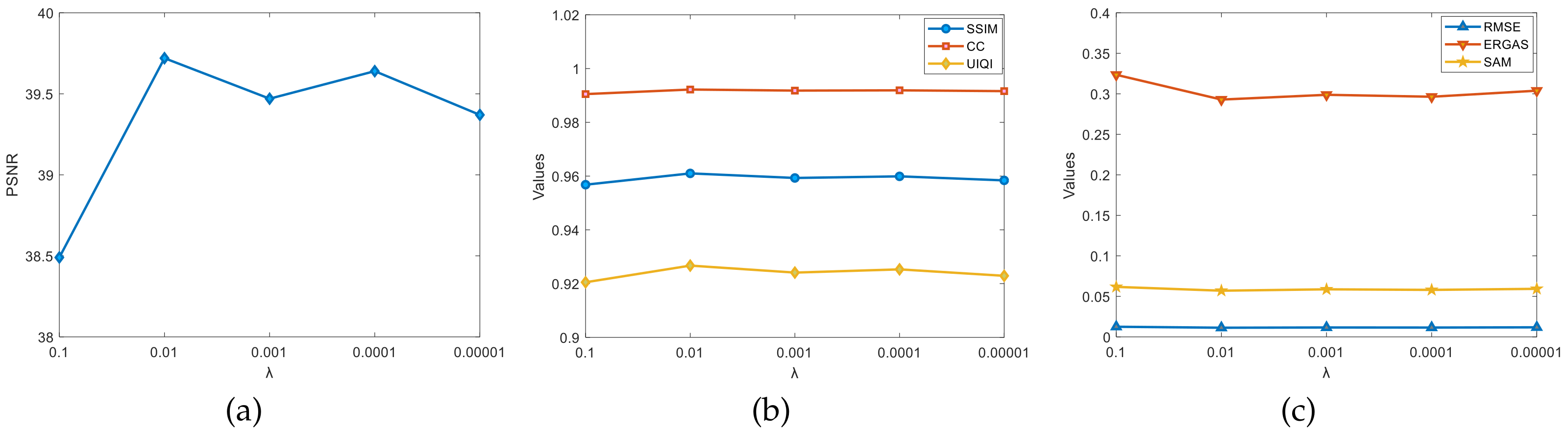
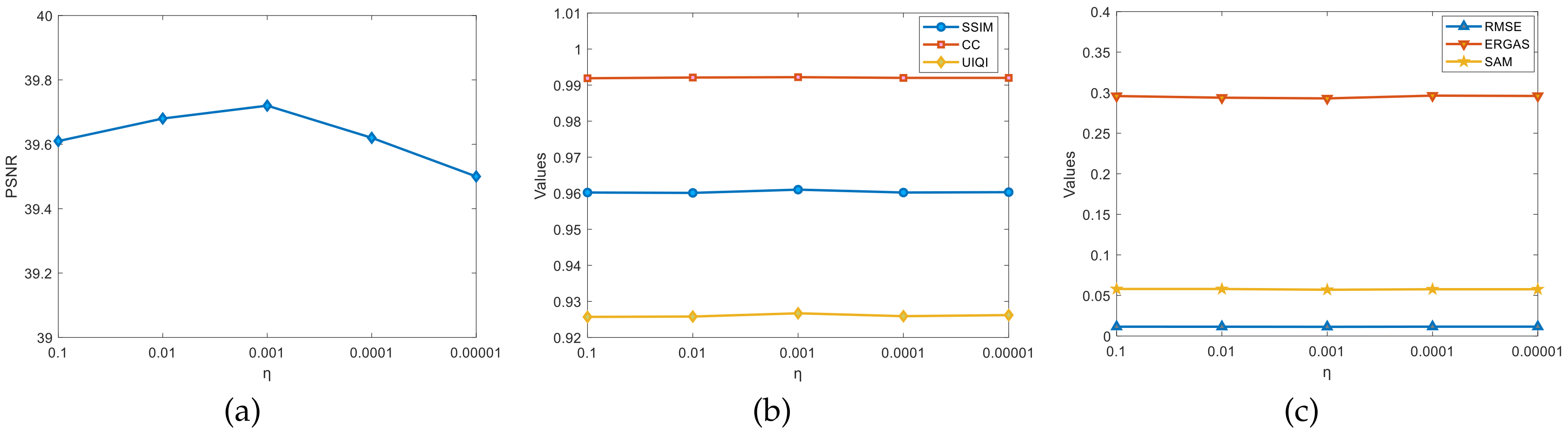
are randomly selected for the experiments to roughly estimate the interval of better results. Secondly, we fix the value of one of the parameters and assign a regular value to the other parameter, observing the changes in the evaluation indicators, such as the PSNR, and finding the better value. Finally, the optimal solution is found around the better value. With the above ideas, the parameter selection process for the Pavia University dataset is given, as shown in
Figure 6 and
Figure 7. By fixing one parameter, the other parameter is scaled down 10 times each time; it was observed that the change in the PSNR and other indexes in the graph was found when
,
, the evaluation indexes reached the optimum, and the algorithm fusion effect was the best. (Note: Other datasets selected the parameter values by this method).
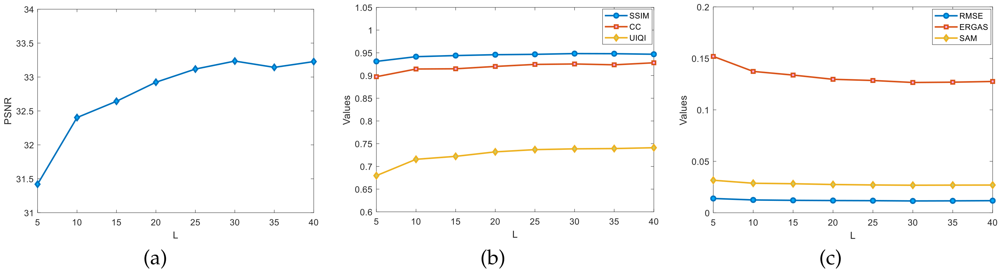
4.5.2. Rough Estimation of the Ranks L and R
For the LL1 fusion-based algorithm, the ranks L and R of the potential factors affect the overall performance of the algorithm. The selection process regarding the ranks L and R of the Pavia University dataset and the Indian Pines dataset are listed here, regarding the data in the experiments are the average of ten independent experiments conducted.
4.5.3. Estimation of L and R on Pavia University Dataset
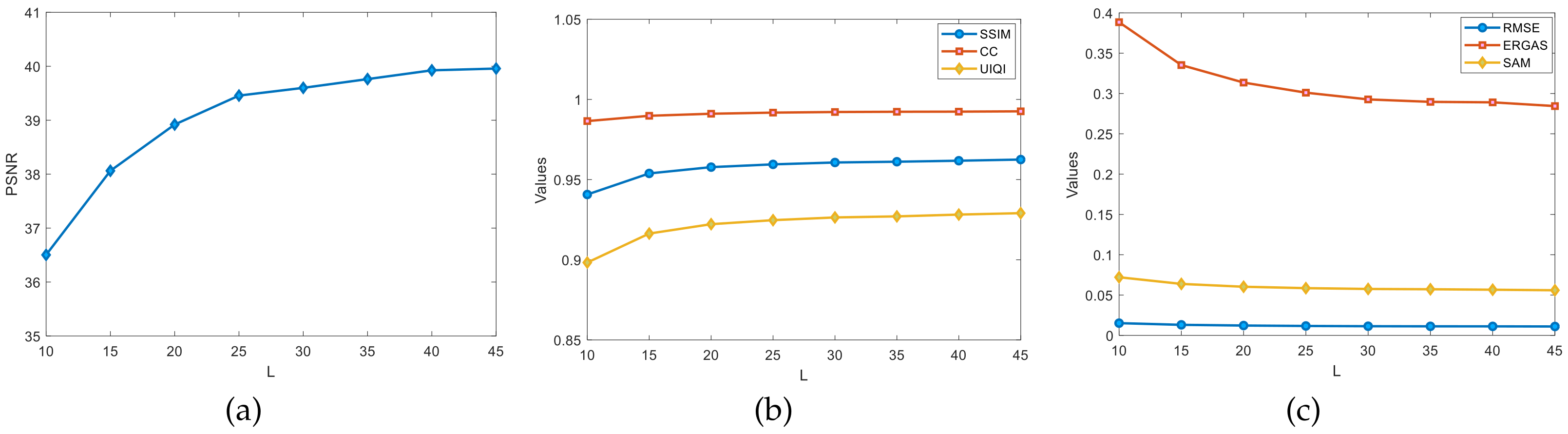
Regarding the rough estimates of the ranks
L and
R in the experiments on the Pavia University dataset, as shown in
Figure 8, the graphs show the changes in the evaluation metrics, such as the PSNR, SSIM, and CC, for different ranks of
L. The
L-value is estimated by fixing the rank
R. Set
here. The
L-value grows at a rate of 5 per increase from 10. It is clearly observed from
Figure 8a that the PSNR values vary more significantly for
L in the
range. The PSNR change remained essentially flat in the
range. In
Figure 8b,
L is in the
range where the three indicators SSIM, CC, and UIQI change more significantly. In summary, it can be roughly estimated that the optimal value of rank
L is around
.
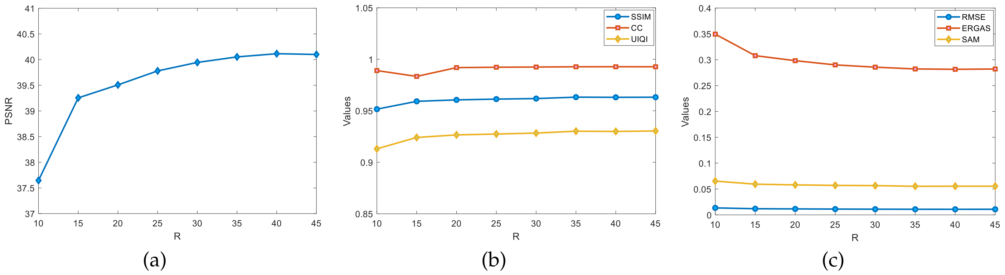
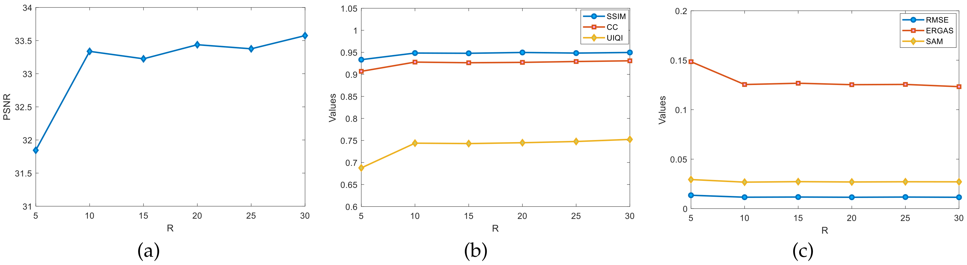
Figure 9 shows the graphs of the variation of evaluation metrics, such as the PSNR, SSIM, and CC, for different ranks of
R in the Pavia University dataset. Fix the rank
L to estimate the R-value, set
, and the
R-value grows at a rate of 5 per increase from 10. As seen in
Figure 9a, the PSNR values increase rapidly with
R in the
range; there is a slow change in the PSNR during the
range; and the PSNR values remained essentially flat in the
range. In
Figure 9b,c, when
R in the
range, the three test metrics of the SSIM, CC, and UIQI improve more significantly, while the RMSE and SAM remain basically stable. In
Figure 9c, there is a significant increase in the ERGAS values in the range
. In the rest of the ranges, all of the tested metrics have basically leveled off without any major improvement. In summary, it can be roughly estimated that the optimal value of the rank
R is around
.
4.5.4. Estimation of L and R on Indian Pines Dataset
Regarding the rough estimates of the ranks
L and
R in the Indian Pines dataset experiment, as shown in
Figure 10, the graphs show the changes in the evaluation metrics, such as the PSNR, SSIM, and CC, for different ranks of
L. Fix the rank
R to estimate
L. Initialize
. The rank
L grows from five at a rate of five per increase. The variation of PSNR values was observed from
Figure 10a where the PSNR values are more significantly improved with
L in the
range. The PSNR appears to decrease in the
range but not significantly. In the
range, it is more stable. In
Figure 10b,c,
L is in the interval of
. The test indexes, such as the SSIM and CC, have more obvious improvements, and, in summary, the optimal value of the rank
L can be roughly estimated to be around
.
Figure 11 shows the graphs of the changes in the evaluation metrics, such as the PSNR, SSIM, and CC, for different ranks of
R on the Indian Pines dataset. Fixing the rank
L estimates
R. By initializing
, the rank
R grows at a rate of five per increase starting from five. Observe the change in the PSNR values from
Figure 11a where the PSNR values were most significantly enhanced by
R in the
range. The PSNR shows more pronounced upward and downward fluctuations in the
range but largely maintains an upward trend. In
Figure 11b,c,
R has a more significant improvement in the test metrics, such as SSIM and CC, in the
range. In the rest of the ranges, the effect is not significantly improved. In summary, an inappropriate choice of the rank
R suppresses the experimental effect of the fusion algorithm, so the optimal value of the rank
R is roughly estimated to be around
.
4.5.5. Signal-To-Noise Ratio Selection
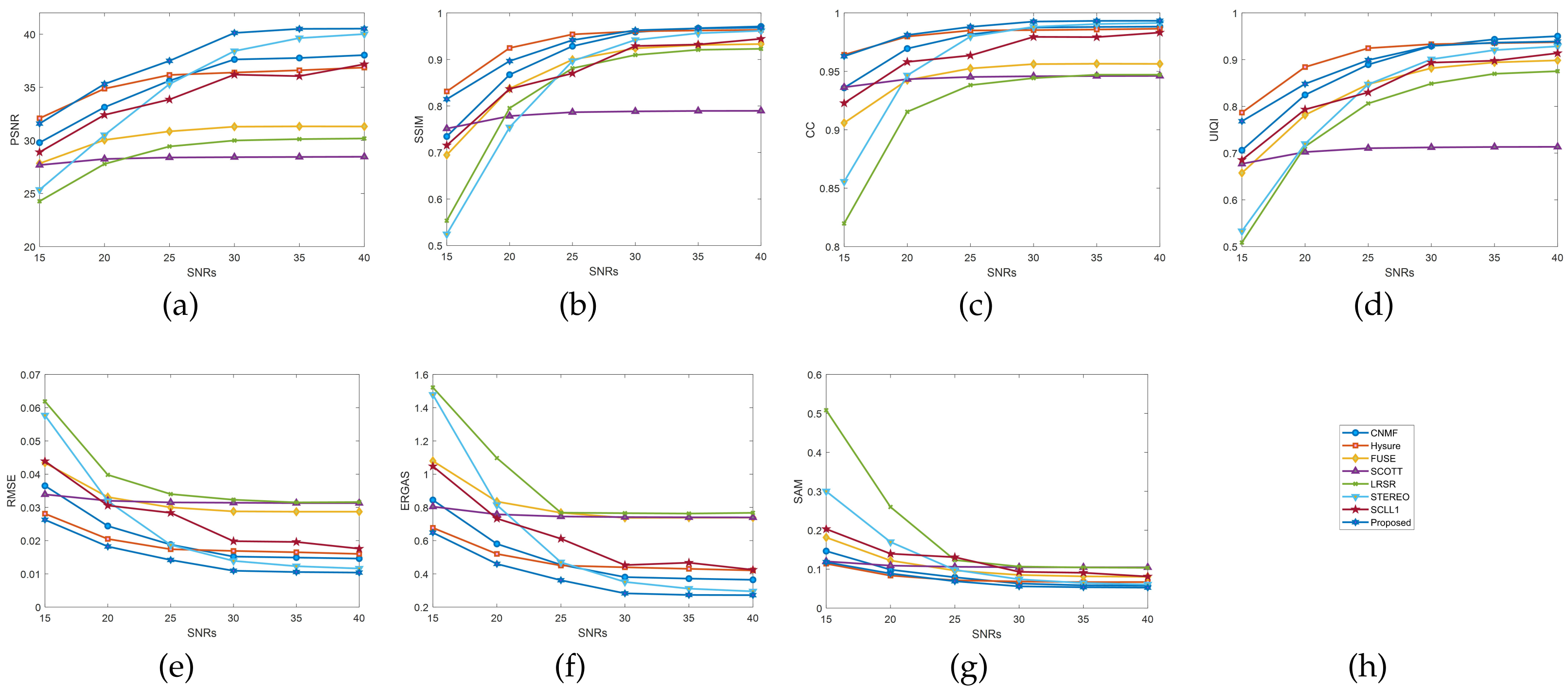
The signal-to-noise ratio (SNR) is also one of the important factors affecting the fusion results of algorithms. The SNR of each algorithm is different, and it is necessary to select an SNR that all algorithms can “accept” to avoid the phenomenon of comparing the optimal and non-optimal results. The selected SNRs (unit: dB) range from
with a 5 dB interval. All experiments were conducted using the Pavia University dataset. The experimental results are shown in
Figure 12. The values of the SNR range is
. Evaluation indicators, such as the PSNR, SSIM, and CC, were significantly improved. In the range
, all evaluation indicators tend to be stable. This shows that the performance of all algorithms is maximally released when
dB.
4.6. Regularization Validity Discussion
A 2D-CNBTD was proposed in previous work [
55], but the algorithm is not perfect and also suffers from low algorithm efficiency, long running time, and noise/artifacts. Therefore, based on the above considerations, a new algorithm (JSSLL1) is proposed in this paper. As shown in
Table 1, the numerical evaluation metrics of the three algorithms, BTD, 2D-CNBTD, and JSSLL1, are given on the Pavia University dataset, Indian Pines dataset, and NingXia Sand Lake dataset, respectively. The better values are indicated in bold, and the time optimum is noted as 0 s. Other evaluation metrics, such as the PSNR and SSIM, are described in
Section 4.3. Among these, the PSNR is used to evaluate the image distortion; the SSIM and UIQI evaluate the spatial features of the fused images; the CC, RMSE, and other metrics are used to evaluate the spectral features of the fused images. From
Table 1, it can be seen that the spatial feature metrics SSIM and UIQI of 2D-CNBTD and JSSLL1 are greatly improved compared with those before improvement. The CC, RMSE, and SAM metrics of the spectral features are also significantly improved. The PSNR is significantly improved as well, which can effectively remove noise from the images. The experimental results of 2D-CNBTD and JSSLL1 on the Pavia University dataset and the NingXia Sand Lake dataset show that the difference between these in the spatial and spectral feature indexes is not obvious; on the NingXia Sand Lake dataset, the PSNR value of JSSLL1 is better; on the Indian Pines dataset, each piece of data for JSSLL1 is closer to the optimal value. In summary, the JSSLL1 algorithm can effectively suppress noise, is suitable for more complex environments, has a lower computational complexity, and can achieve the goal in the least amount of time.
4.7. Standard Dataset Experimental Results and Discussion
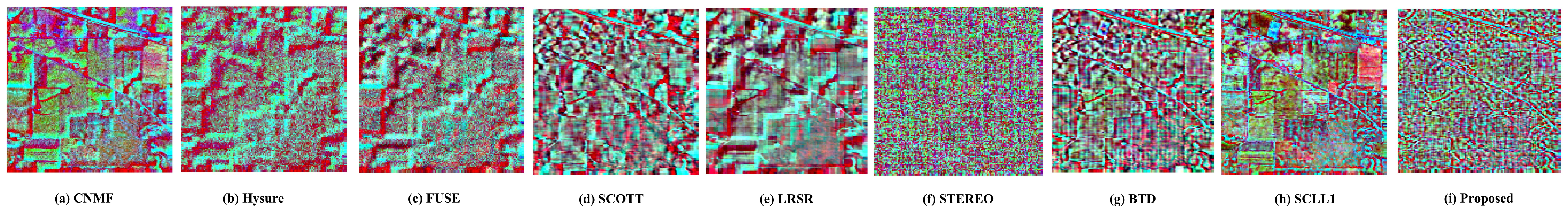
This section shows the experimental results of the eight fusion algorithms on the Pavia University dataset and the Indian Pines dataset. The experimental results include visual images of the fusion results, difference images, and the numerical results of evaluation metrics.
4.7.1. Pavia University Dataset Experimental Results and Discussion
Through the above experiments, the parameters of the Pavia University dataset are set as:
,
, and
dB. Due to the specificity of the model in this paper, the estimation and selection of the rank can be “overestimated”, so the roughly estimated ranks R and L are slightly adjusted upwards and set to:
,
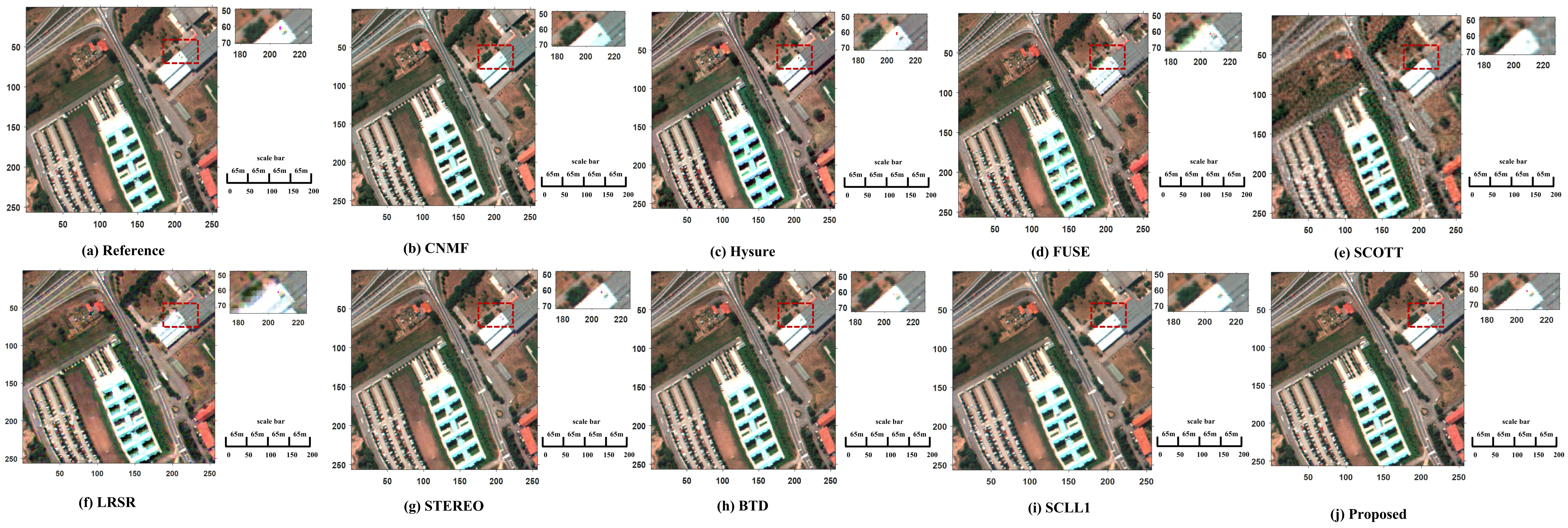
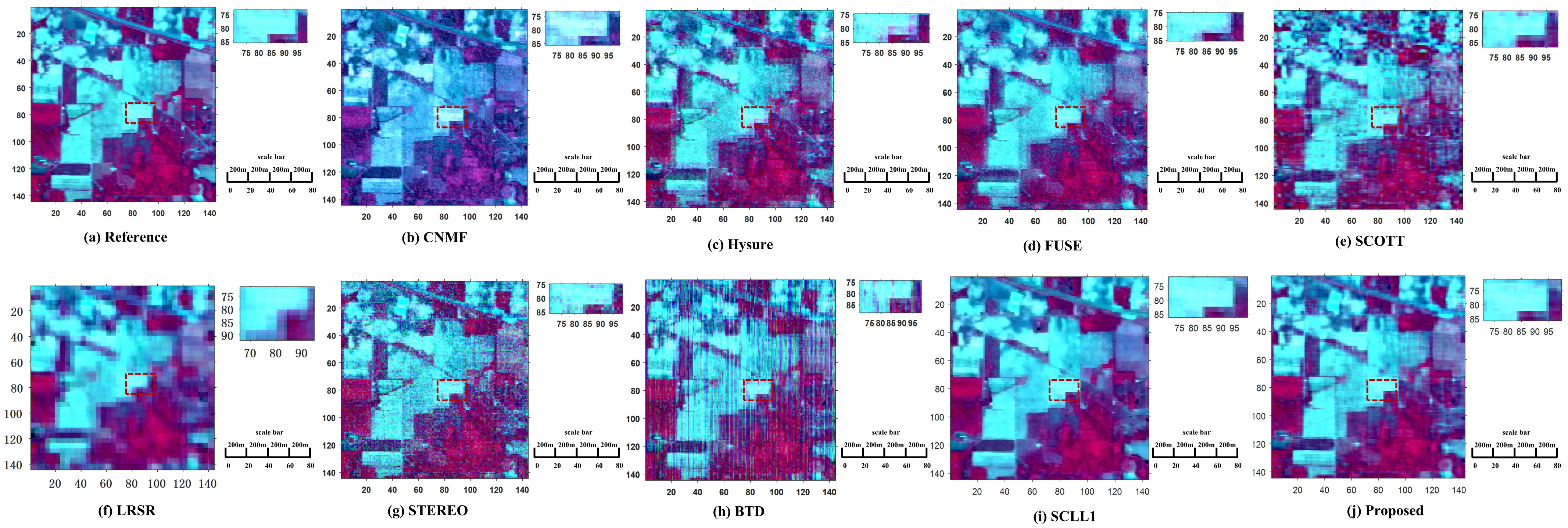
. The algorithm superiority was evaluated by observing the visualized images. For the Pavia University dataset, the three bands 61, 25, and 13 were selected as the red, green, and blue bands, respectively, and fused to generate pseudo-color images. The HRHS is shown in
Figure 13.
Figure 13a shows the original image of the Pavia University dataset. In order to see the differences in HRHSs more clearly, the red box part in each HRHS image is enlarged, and the enlarged part is shown in the upper right corner. The difference images of all algorithms are shown in
Figure 14.
As can be seen in the enlarged part shown in
Figure 13, compared with the reference image, some spatial information is lost in the HRHS image of CNMF; a large number of blurred blocks and noise appear in the fusion result of SCOTT, and the spatial information is seriously missing; the fusion results of SCLL1 and the BTD are clearer; no blurred blocks and noise are seen, but some spatial information is lost. The HySure and STERE fusion results in a low loss of spectral and spatial information; no noise and blurred blocks are seen in the fusion results of the algorithm proposed in this paper, and the spatial information is also preserved.
Figure 14 shows the difference images obtained after the difference between the target image and the fused image. Among these, the difference images of CNMF, Hysure, FUSE, LRSR, and SCLL1 have a lot of texture information; SCOTT has less texture information; the difference images of STEREO, the BTD, and the algorithm of this paper are more similar and do not see more texture information, but, in comparison, STEREO and the BTD still have some building outline information.
When the PSNR is greater than 30 dB, it is difficult to observe the difference in the images with the naked eye, and the algorithm needs to be evaluated in terms of both the spectral and spatial features with the help of some evaluation metrics. The evaluation indexes of the Pavia dataset are shown in
Table 2. As can be seen from the data in the table, the metrics describing the spectral and spatial information, the SSIM, CC, RMSE, ERGAS, and SAM of the algorithm in this paper, are closer to the optimal values, and only the UIQI is slightly inferior to the CNMF algorithm, which means that the algorithm in this paper performs the best in terms of spatial information, spectral information, image contrast, and brightness in the process of reconstructing images. In terms of the PSNR values, this paper’s algorithm can effectively reject noise. Under the same number of iterations and in the same environment, the running time of this paper’s algorithm, compared with the BTD and SCLL1, has been significantly improved.
4.7.2. Pavia University Dataset Classification Experimental Results and Discussion
Image classification is one of the important application scenarios for high-resolution hyperspectral images. Acquiring high-resolution hyperspectral images is another important purpose of image fusion. A high-quality fused image will make the classification experiment “half the work”. The experimental data contain information about buildings, vegetation, roads, bare soil, and other features. Therefore, a lightweight spectral–spatial convolutional network (
) [
73] with a low complexity and few network parameters was chosen to perform classification experiments on the fused images from Pavia University, as well as the original images for each algorithm. A 3 × 3 deep convolutional (Conv) filter was used for the experiments, and a filter with a convolution kernel of 1 × 1 was chosen for spectral feature extraction. A 3 × 3 filter was chosen for spatial feature extraction. All other parameter settings in this paper follow the literature [
73]. Each experiment was repeated ten times. The results of the classification experiments on the Pavia dataset are shown in
Table 3.
As shown in
Table 3, the HRHS image classification results of each algorithm are shown by the evaluation index. It should be specifically noted here that the HRHS of CNMF, Hysure, and the other algorithms are obtained by downsampling the original image, so the closer the classification result is to the original image, the better the classification result will be. Therefore, compared with other algorithms, the HRHS classification result data of the algorithms in this paper, STEREO and the BTD, are closer to the reference image; the HRHS image classification effects of CNMF and Hysure are the second, and the HRHS image classification effects of FUSE, SCOTT and SCLL1 are the worst.
4.7.3. Indian Pines Dataset Fusion Experiment Results and Discussion
The parameters for the Indian Pines dataset are set to
,
, and
dB. Due to the specificity of the model in this paper, the estimation and selection of the rank can be “overestimated”, so the roughly estimated ranks
R and
L are slightly adjusted upward and set to
,
. Here, the three bands 61, 25, and 13 are selected as the red, green, and blue bands, respectively, and fused to generate pseudo-color images. The HRHS is shown in
Figure 15, and
Figure 15a shows the original image of the Indian Pines dataset. To see the differences in the HRHS more clearly, the red-boxed part of each HRHS plot is enlarged, and the enlarged part is shown in the upper right corner. The difference images for all algorithms are shown in
Figure 16.
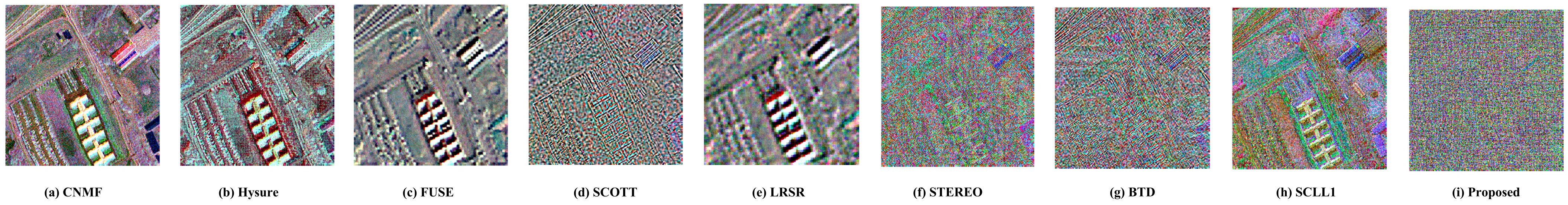
As can be seen in the enlarged part shown in
Figure 15, compared with
Figure 14a, the HRHS of CNMF appears distorted; the HRHS of Hysure, SCOTT, STEREO, and the BTD has a large fuzzy block and noise with serious loss of spatial information. The HRHS of FUSE, SCLL1, and this paper’s algorithm is clear; neither noise nor fuzzy block are seen, and the loss of spatial information is less.
Figure 16 shows the difference images of each algorithm on the Indian Pines dataset. Among these, the difference images of CNMF, Hysure, FUSE, SCOTT, LRSR, the BTD, and SCLL1 show a lot of spatial texture, indicating that there is a serious loss of spatial information in the HRHS obtained by the above algorithms; the difference images of STRTEO and the algorithms in this paper do not show more spatial texture, indicating that the HRHS images of these two algorithms are closer to the reference image.
The data in
Table 4 show that among the metrics describing the spectral and spatial information, the UIQI, CC, RMSE, ERGAS, and SAM of this algorithm are closer to the optimal values, and only the SSIM is slightly inferior to the SCLL1 algorithm, indicating that this algorithm loses less spatial and spectral information in the process of reconstructing images, and the HRHS fused images are closer to the original dataset. In terms of the PSNR, this algorithm can better suppress noise; meanwhile, compared with the BTD and SCLL1, the running time of this algorithm is shorter.
4.8. Local Dataset Fusion Experimental Results and Discussion
The Ningxia Sand Lake dataset was acquired by two high-resolution satellites over the Sand Lake successively, and, here, the original dataset has been aligned and corrected by ENVI 5.3 software. By experimental verification,
and
are not changed.
R and
L are set as
,
. Then, the three bands, 59, 38, and 20, are selected as the red, green, and blue bands, respectively, and fused to generate pseudo-color images. The HRHS is shown in
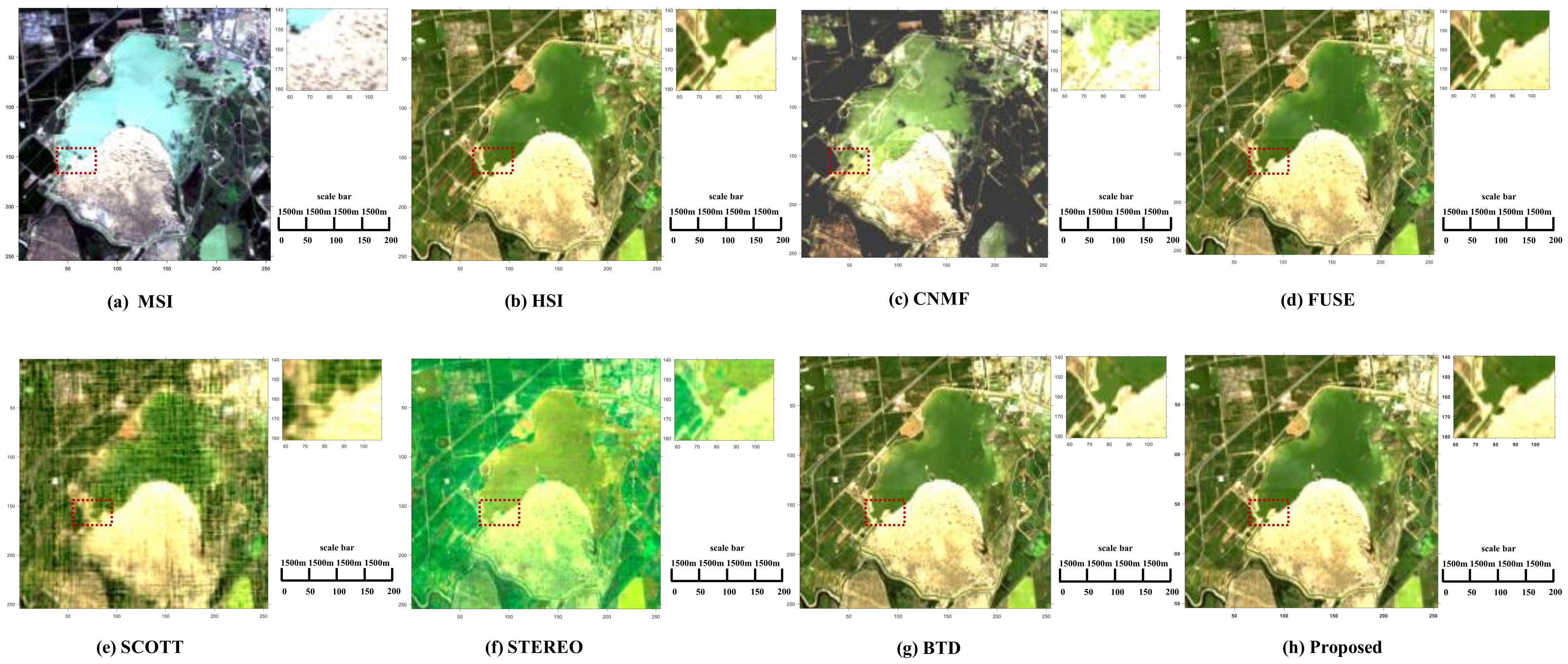
Figure 17.
Figure 17a,b show the HR-MSI and LR-HSI acquired by the satellites, respectively. In order to see the HRHS differences of each algorithm more clearly, each red boxed part of the HRHS plot is enlarged, and the enlarged part is shown in the upper right corner.
As can be seen from the enlarged part in
Figure 17, compared with the reference image, the HRHS of CNMF and STEREO showed distortion. The presence of a great number of fuzzy blocks and noise in the HRHS images of SCOTT and STEREO, shows that their spatial information was lost in the fusion process; the HRHS of FUSE and the BTD showed a small number of blurred blocks. In comparison, the HRHS of the algorithm in this paper was clearer; neither noise nor blurred blocks were seen, and less spatial information was lost.
The Hysure and SCLL1 algorithms show outliers when experimenting on the NingXia Sand Lake dataset, and the LRSR algorithm also requires downsampling of the collected dataset for local dataset experiments, which is referred to as “pseudo-fusion”, while the algorithm in this paper directly fuses the two images. Therefore, these three algorithms are not compared. The numerical data of the other algorithms are shown in
Table 5. Bold means the best value. Among the indicators describing the spatial and spectral information, the UIQI, CC, RMSE, ERGAS, and SAM of the algorithms proposed in this paper are closer to the optimal values, and the SSIM is a little smaller than the BTD numerical indicators. This means that the algorithm in this paper can retain the spatial structure and spectral information in LR-HSI and HR-MSI images well during the process of reconstructing HRHS images; the PSNR value is also the highest, which shows that the proposed algorithm also performs well in suppressing noise.
4.9. Analysis of Algorithm Complexity
The computational complexity of this model primarily involves matrix operations and element-wise computations. To calculate the complexity of the model, we can analyze the computational cost of each term and sum them up.
Each term in the model involves both matrix operations and element-wise computations. Specifically, the model consists of the following components:
First term: . Second term: . Regularization term: .
For each term, we can separately consider the computational complexity of matrix operations and element-wise computations.
The first term involves matrix multiplication, element-wise multiplication, and summation. The most time-consuming part is the matrix multiplication. Assuming has dimensions , and have dimensions and , and and are dimension-adaptation matrices. The matrix multiplication has a complexity of approximately , followed by element-wise multiplication and summation with a complexity of .
The second term is similar to the first term, involving matrix multiplication, element-wise multiplication, and summation. Assume has dimensions , and have dimensions and , and is a dimension-adaptation matrix. The matrix multiplication has a complexity of , followed by element-wise multiplication and summation with a complexity of .
The regularization term involves element-wise operations such as squaring, square root, summation, and multiplication. Assuming each vector , , and has a dimension of K, the computational complexity for each r is approximately , resulting in a total complexity of .
Therefore, adding up the complexities of these three components, the overall computational complexity of the model is approximately .


