Article

A Machine-Learning-Based Study on All-Day Cloud Classification Using Himawari-8 Infrared Data

1
School of Remote Sensing and Information Engineering, North China Institute of Aerospace Engineering, Langfang 065000, China
2
Hebei Collaborative Innovation Center for Aerospace Remote Sensing Information Processing and Application, Langfang 065000, China
3
Aerospace Information Research Institute, Chinese Academy of Sciences, Beijing 100094, China
*
Author to whom correspondence should be addressed.
These authors contributed equally to this work.
Remote Sens. 2023, 15(24), 5630; https://doi.org/10.3390/rs15245630
Submission received: 14 October 2023 / Revised: 17 November 2023 / Accepted: 1 December 2023 / Published: 5 December 2023

Abstract

:
Clouds are diverse and complex, making accurate cloud type identification vital in improving the accuracy of weather forecasting and the effectiveness of climate monitoring. However, current cloud classification research has largely focused on daytime data. The lack of visible light data at night presents challenges in characterizing nocturnal cloud attributes, leading to difficulties in achieving continuous all-day cloud classification results. This study proposed an all-day infrared cloud classification model (AInfraredCCM) based on XGBoost. Initially, the latitude/longitude, 10 infrared channels, and 5 brightness temperature differences of the Himawari-8 satellite were selected as input features. Then, 1,314,275 samples were collected from the Himawari-8 full-disk data and cloud classification was conducted using the CPR/CALIOP merged cloud type product as training data. The key cloud types included cirrus, deep convective, altostratus, altocumulus, nimbostratus, stratocumulus, stratus, and cumulus. The cloud classification model achieved an overall accuracy of 86.22%, along with precision, recall, and F1-score values of 0.88, 0.84, and 0.86, respectively. The practicality of this model was validated across all-day temporal, daytime/nighttime, and seasonal scenarios. The results showed that the AInfraredCCM consistently performed well across various time periods and seasons, confirming its temporal applicability. In conclusion, this study presents an all-day cloud classification approach to obtain comprehensive cloud information for continuous weather monitoring, ultimately enhancing weather prediction accuracy and climate monitoring.

1. Introduction

Cloudiness, a consequence of the presence of minuscule water vapor particles or ice crystals in the atmosphere, is closely intertwined with numerous climatic phenomena [1]. According to the International Satellite Cloud Climatology Project [2,3], the global annual average cloud cover covers two-thirds of the Earth’s surface. As the primary regulators of the Earth’s radiation balance, the water cycle, and biogeochemical cycles [4,5], distinct cloud types produce varying radiative effects. Therefore, the precise categorization of cloud types and understanding of their distribution patterns hold significant practical importance [6,7]. The pursuit of effective and precise cloud classifications remains a prominent focus in meteorological research [8].
In past decades, cloud classification has predominantly been carried out using traditional methods and machine-learning-based techniques. Traditional methods include thresholds and statistical mathematical methods. However, these methods rely heavily on empirical knowledge when dealing with data, resulting in low classification efficiency. With continuous developments in computer science, several machine learning methods have emerged. Machine learning methods do not require extensive prior knowledge and offer high computational efficiency and excellent classification performance [9]. Therefore, conventional machine learning methods such as Random Forest (RF) and Support Vector Machine (SVM) approaches have been widely used in cloud classification research [10]. Wohlfarth et al. [11] used data from three visible channels and one infrared (IR) channel obtained from the Landsat-8 satellite. They classified clouds into nine different cloud classes and four subsurface classes using the SVM algorithm, achieving an impressive classification accuracy of up to 95.4%. Yu et al. [12] proposed a cloud classification method based on an RF algorithm for FY-4A. This method was combined with CloudSat’s 2B-CLDCLASS cloud product to classify 8 single-layer cloud types and 12 multilayer cloud types. As the volume of data continues to increase, deep learning models such as deep neural networks (DNN) and artificial neural networks (ANN) are increasingly being used in cloud classification research. Cai et al. [13] employed FY-2C’s infrared channel 1 (10.3–11.5 μm) data in combined with a Convolutional Neural Network (CNN) model for cloud classification. Their classification divided clouds into 5 types, achieving an impressive average recognition rate of 90.6%. In addition, Gorooh et al. [14] proposed the Deep Neural Network Cloud-Type Classification (DeepCTC) model that can classify clouds into 8 different types with an overall classification accuracy of 85%. Machine learning techniques have surpassed traditional cloud classification methods in terms of both classification speed and accuracy. However, it is important to note that these methods are generally applicable to daytime cloud classification. Nighttime visible light data are often noisy and cannot be used for nighttime cloud classification. Therefore, one of the research questions addressed in this study is how to achieve nighttime cloud classification.
Researchers have commenced extensive studies using infrared data to more accurately monitor cloud evolution at night, eliminating the need for visible data and achieving successful research outcomes [15]. Tan et al. [16] proposed a nighttime cloud classification algorithm based on Himawari-8 satellite channel data and machine learning algorithms. They utilized data from 5 infrared channels, 3 brightness temperature difference (BTD) datasets, and latitude/longitude information as training features. By employing the RF algorithm, this approach achieved an overall accuracy of 0.79, classifying clouds into clear-sky, single-layer, and multilayer clouds. Li et al. [17] used infrared data from the Himawari-8 satellite to classify clouds. Their classification scheme included five types: clear, single-ice clouds, single-mixed clouds, single-water clouds, and multilayer clouds. They achieved an impressive overall classification accuracy of 0.81. Despite significant progress in nighttime cloud classification research, a critical analysis of existing research results revealed a limited number of nighttime cloud classifications. Typically, cloud classification is constrained to primary cloud categories without considering the finer distinctions between clouds.
This study addresses the challenges of nighttime cloud classification and the limited number of classifiers using the latitude/longitude, five brightness temperature differences (BTD), and ten IR channels from the Himawari-8 satellite. The combined Cloud-Profiling Radar (CPR) and Cloud-Aerosol LIDAR with Orthogonal Polarization (CALIOP) cloud-type product 2B-CLDCLASS-LIDAR were used as labels, which classified clouds into nine types: clear-sky (Clear), cirrus (Ci), deep convective (Dc), altostratus (As), altocumulus (Ac), nimbostratus (Ns), stratocumulus (Sc), stratus (St), and cumulus (Cu). By comparing various models using various metrics, such as overall accuracy, precision, recall, and F1-scores, this study investigated the viability of all-day cloud classification and the selection of optimal parameters. The goal was to improve both the quantity and accuracy of cloud classification, thus providing valuable additional reference data for nighttime meteorological observations.
Section 2 introduces the experimental data and methodology used in this study. Section 3 presents the experimental results and their implications. Finally, Section 4 and Section 5 present the discussion and conclusion, respectively.

2. Materials and Methods

2.1. Data Collection

This study used Level-1 infrared channel data from the Himawari-8 satellite and the cloud type product 2B-CLDCLASS-LIDAR, which is a joint project of CloudSat and CALIPSO. Additionally, longitude, latitude, and solar zenith angle data were employed for support.
(1)
Himawari-8 data
The Japan Meteorological Agency’s Geostationary Meteorological Satellite, Himawari-8, was launched on 7 July 2015. The data from this satellite can be accessed through the Japan Aerospace Exploration Agency (JAXA) (http://www.eorc.jaxa.jp/ptree/index.html, accessed on 15 May 2023) [18]. Compared with MTSAT-2 (Himawari-7), Himawari-8 is equipped with an Advanced Himawari Imager (AHI) sensor that has expanded from the original 5 bands to 16 bands, including 3 visible light bands, 3 near-infrared bands, and 10 infrared bands [19,20]. It covers the area from 60°S to 60°N and from 80°E to 200°E (Figure 1). The observation frequency of Himawari-8 has been increased to once every 10 min, providing abundant data for meteorological studies and continuous cloud observations [21]. This study used 10 infrared bands from the Himawari-8 satellite. Table 1 displays the parameters of the 10 infrared bands of the Level-1 products of Himawari-8 and their main applications.
The Level-2 (L2) cloud product of the Himawari-8 satellite provides a comprehensive set of cloud-related parameters, such as cloud type (CLTYPE), cloud top height, cloud top temperature, and cloud optical thickness. However, it is important to note that this product solely provides cloud information for observations made during the daytime period. The spatial resolution is 5 km and the temporal resolution is 10 min. A more detailed description of AHI Level-1/2 data is available at https://www.eorc.jaxa.jp/ptree/userguide.html, accessed on 20 June 2023.
This study used 10 infrared bands as basic data, ranging from band 7 to band 16. In addition, auxiliary data, including longitude, latitude, sun zenith angle, and CLTYPE, were incorporated. Figure 2 displays the cloud images of Himawari-8 satellite for its 10 infrared channels at UTC 03:20 on 1 July 2019.
(2)
CloudSat data
CloudSat and CALIPSO are part of the A-train that crosses the equator in the afternoon [22]. Both satellites provide near global views of clouds from sun-synchronous orbits and are available at https://www.cloudsat.cira.colostate.edu, accessed on 23 May 2023. CloudSat’s onboard CPR and CALIOP (a vision and near-infrared LIDAR) are 2 powerful onboard active instruments [23]. Currently, these are the only instruments capable of accurately detecting the vertical structure of clouds [24]. Owing to the different working wavelengths of CPR and CALIOP, they exhibit different sensitivities to different types of clouds. The millimeter-wave radar CPR has the advantage of detecting optically thick clouds and precipitation systems [25]. Combining their advantages, a joint product of CPR/CALIOP was developed to provide the most reliable vertical cloud information; this was named 2B-CLDCLASS-LIDAR. This product provides information on up to 10 cloud layers. These layers are characterized by a horizontal resolution of 1.4 × 1.8 km and a vertical resolution of 0.24 km. This dataset contains valuable details, including cloud layers, cloud heights, and cloud phases [26]. The CloudLayerType band elements range from 0 to 8 and represent different cloud types: Clear, Ci, As, Ac, St, Sc, Cu, Ns, and Dc. In this study, CloudLayerType band data were utilized as the labeling criteria. For a more comprehensive understanding of 2B-CLDCLASS-LIDAR, please refer to the CloudSat product brochure [27].
(3)
Cloud type of this study
In this study, 130 days of data (Table A1) were selected from November 2018, January 2019, March 2019, June 2019, and July 2019. The Himawari-8 CLTYPE products encompass 10 types (0–9 represent Clear, Ci, Cs, Dc, Ac, As, Ns, Cu, Sc, and St, respectively) and CPR/CALIOP products consist of only 9 types. To ensure consistency, the clouds were finally classified into 9 types based on the one-to-one mapping between the CPR/CALIOP and Himawar-8 clouds. Notably, in Himawari-8, Ci and Cs were merged into a one type called Ci clouds. The classification criteria are listed in Table 2.

2.2. Method

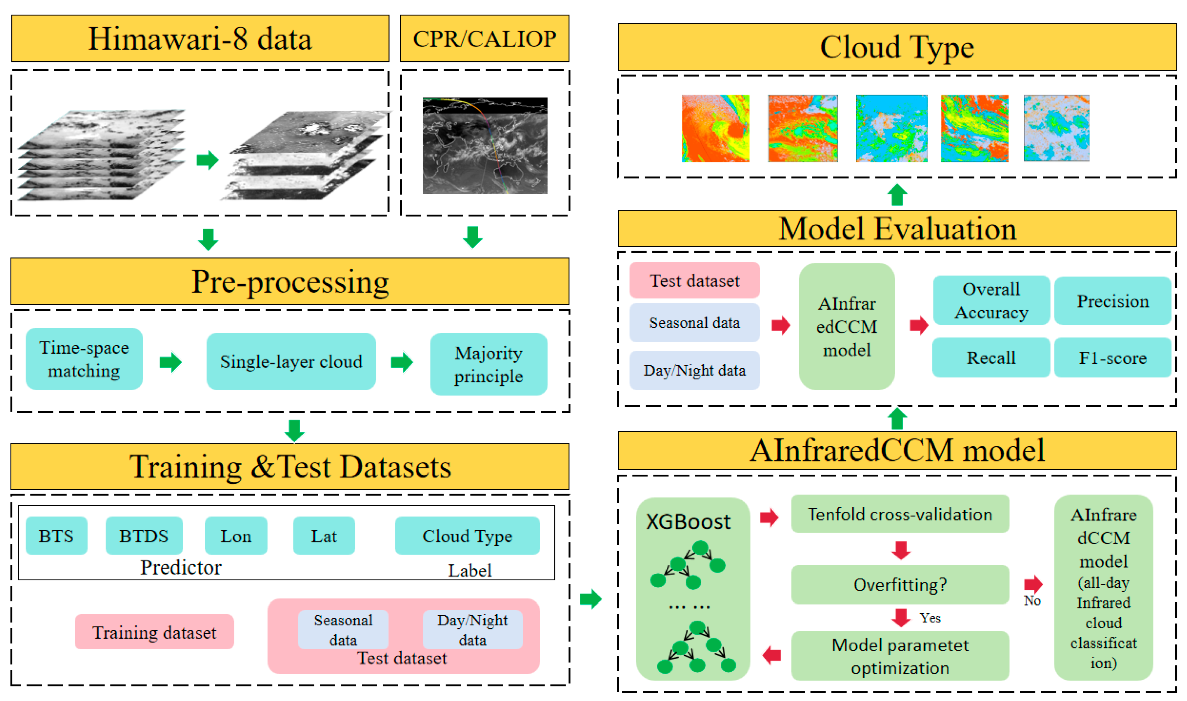
In this study, 10 different IR bands from Himawari-8 and 5 BTDs were used to select potential donor pixels. Longitude and latitude were used as additional constraints. In the following section, the proposed algorithm is referred to as the All-day Infrared Cloud Classification Model (AInfraredCCM). Figure 3 shows a conceptual diagram of the method used in this study and its comparison.
(1) Data collection and processing: This study utilized various sources, such as CloudLayerType, Himawari-8 Level-1 IR, latitude and longitude, and solar zenith angle data from the 2B-CLDCLASS-LIDAR product [26]. To obtain BTD information, pairwise differences were calculated between all the infrared channels. Subsequently, feature selection was performed using the feature analysis function within the machine learning module [28]. The final input feature set included 5 BTDs, 10 infrared channels, and latitude and longitude data. BTD (11.2–7.3 μm) can be employed to detect high- and mid-level clouds over land during the night. BTD (3.9–11.2) is known as useful BTD to detect low-level clouds. BTD (11.2–12.4 μm) is useful for distinguishing thin clouds from clear sky. BTD (12.4–10.4 μm) can serve as a substitute for visible light to describe cloud optical thickness. BTD (7.3–10.4 μm) is utilized for nighttime cloud detection by differencing the water vapor channel and the infrared channel [10,29]. After obtaining the BTD data, a series of data preprocessing steps were applied to both the Himawari-8 and CPR/CALIOP datasets. These steps include spatiotemporal matching, label extraction, data resampling, and cropping. Consequently, a training dataset consisting of 1,182,688 samples and a testing dataset consisting of 131,587 samples were created following a random 9:1 split ratio. The specific features contained in the dataset are listed in Table 3.
(2) Label extraction: To obtain cloud type samples for training, Himawari-8 and 2B-CLDCLASS-LIDAR products were subjected to temporal and spatial matching. Each pixel in the CloudLayerType dataset contained information on 10 cloud types, and each Himawari-8 pixel corresponded to a cloud type. During data matching, the first step was to compress the 10-layer data. If the CPR point corresponded to multilayer clouds with different cloud types in each layer, it was defined as a multilayer cloud; otherwise, it corresponded to the cloud type in the first layer. The second step involved a temporal and spatial matching process due to the difference in the spatial and temporal resolutions between AHI and CPR. This entailed selecting AHI data points within a 5 min time window of the CPR scan point and within a 5 km radius of the CPR point location [30,31]. In the third step, considering that the AHI observations did not include multilayer cloud types, the CPR points corresponding to multilayer clouds were eliminated. Finally, cloud type labels were assigned by majority rule based on the matching of AHI and CPR points [32,33].
(3) Model building: The processed dataset was used to train the XGBoost model, and the optimal model parameters were determined by Bayesian optimization. This step selection was made by sampling using the Bayesian optimization algorithm after estimating the distribution of the objective function in the parameter space through a Gaussian process model. It evaluated the overall classification accuracy of related models while searching for the best parameter combination across a finite number of iterations. Finally, the parameter combination with the highest overall classification accuracy was obtained and represented as the optimal model parameters.
(4) Model evaluation: The overall accuracy (OA), precision, recall, and F1-score were calculated based on ten-fold cross-validation [34]. If the final model achieved sufficient accuracy, it was selected; otherwise, the parameters were modified.
This study used the parameters shown in Table 4 as an example to better explain the metrics used for accuracy assessment. Assume that a dataset C consists of T samples; here, AS is the number of samples for class A clouds and BS is the number of samples for class B clouds. Table 4 shows the specific classification results from dataset C, which were used for model classification prediction.
The overall accuracy (OA) is a crucial measure, representing the proportion of correctly classified samples to the total number of samples [12]. A higher overall accuracy indicates a more reliable classification outcome. The overall accuracy is calculated as follows:
O A = T A + T B T A + F B + F A + T B
where TB represents an accurately classified cloud type B.
Precision is a metric that quantifies the proportion of correctly identified clouds in the target class, indicating fewer classification errors. Precision can be expressed as follows:
P r e c i s i o n = T A T A + F A
where TA denotes correctly identified class A clouds and FA denotes the misdiagnosis of class A clouds as class B clouds.
The recall pertains to the proportion of correctly identified class A clouds within the total number of identified class A clouds [35]. Recall can be represented as follows:
R e c a l l = T A T A + F B
where TA denotes the correct identification of class A clouds and FB denotes the misdiagnosis of class B clouds as class A clouds.
The F1-score combines precision and recall, with values ranging from 0 to 1. A higher score indicated that the model was more accurate. Compared with that using only precision or recall metrics, this score provides a more comprehensive evaluation of model accuracy [36]. The F1-score can be written as follows:
F 1 = 2 P r e c i s i o n R e c a l l P r e c i s i o n + R e c a l l
(5) The AInfraredCCM was conducted through all-day cloud classification for the entire research area using the test data.
XGBoost is an ensemble learning method that employs boosting principles. Unlike traditional boosting methods, XGBoost uses tree models (decision trees) as weak learners. It combines multiple weak learners to create a strong learner, gradually improving the model’s performance. XGBoost is adaptive; in each iteration, it introduces a new weak classifier that attempts to correct the errors of the previous round until the stopping condition is satisfied. The key characteristic of XGBoost is the integration of multiple weak learners into a strong learner, gradually improving the model accuracy through iterative error correction [37].
Bayesian optimization approach was employed to tune the model and identify the optimal parameters of the AInfraredCCM model. The n_estimators parameter was set within a range from 100 to 300, the learning_rate parameter was set within a range from 0.01 to 0.999, the max_depth parameter was set within a range from 10 to 100, and the min_child_weight parameter ranges from 1 to 10 during optimization. After 100 iterations, the AInfraredCCM was developed, and the model parameters are displayed in Table 5.

3. Results

3.1. Comparison with Other Methods

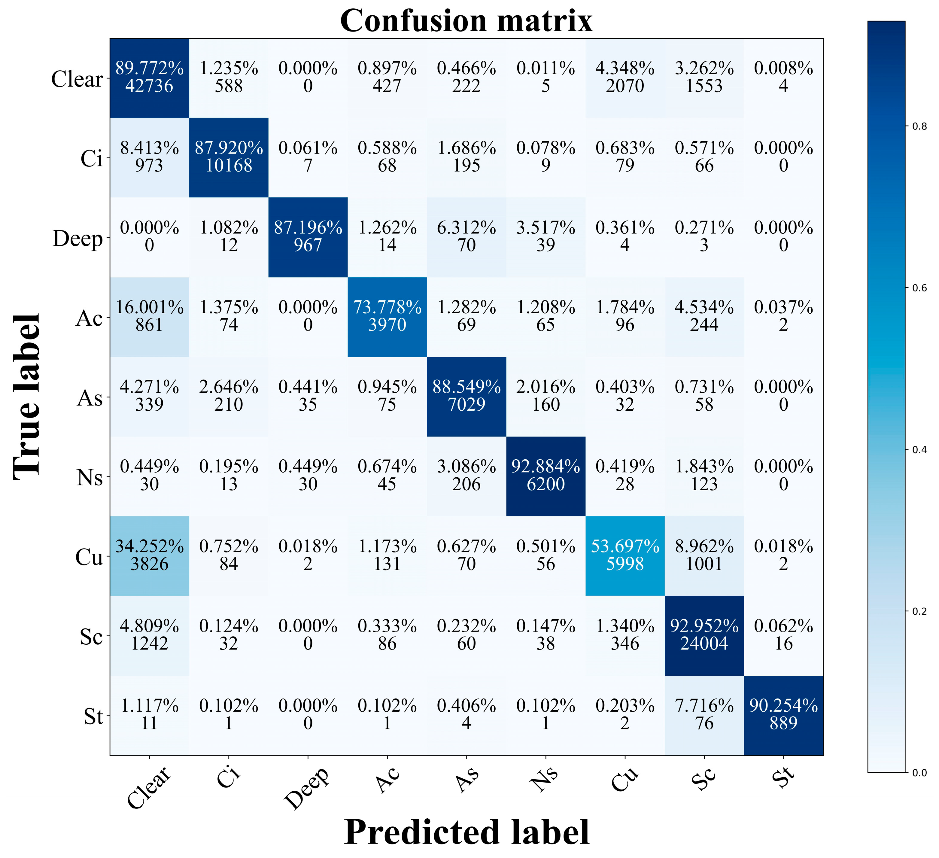
The results are based on an independent test dataset of approximately 130,000 pixels, which is divided into clear sky and eight different cloud forms. Table 6 shows the precision, recall, and F1-score of the AInfraredCCM for each form of cloud in the training dataset. The confusion matrix for various types of clouds is shown in Figure 4, wherein the vertical coordinate represents the true value and the horizontal coordinate represents the predicted value.
Based on the model’s classification results for the all-day data, the average overall accuracy for all cloud types was 86.22%, with a precision of 0.88, a recall of 0.84, and an F1-score of 0.86. Notably, Cu clouds exhibited considerably lower identification rates than the other cloud types, and both recall and F1-score are significantly lower than those of other cloud types (Table 6). The confusion matrix shown in Figure 4 graphically displays that most of Cu is misclassified as clear sky (34.252%) and Sc (8.962%). These phenomena can be attributed to the unique properties of Cu, which include two possibilities: one resembles Cu in clear weather and appears as thin, fragmented clouds that closely resemble clear in terms of reflectance, making them easy to misidentify; the alternative scenario is continuous Cu, which is denser and more vertically developed than clear-sky Cu and is frequently categorized as Sc.
To enhance the credibility of the model, the cross-validation results were compared with those obtained using various other models, including RF, LightGBM, AdaBoost, and GradientBoost. RF is a conventional machine learning model known for its versatility in handling both classification and regression tasks. LightGBM has been optimized for large datasets, offering high processing speed and low memory usage. This makes it particularly suitable for scenarios involving substantial amounts of data and high dimensional features [38]. Gradient Boosting is a boosting-based integrated learning technique known for its robustness to outliers and good performance in a variety of classification and regression problems. Similarly, AdaBoost is an integrated learning method that employs weighted voting to combine several weak classifiers. The weights are updated after each iteration based on the outcome of the previous round, thereby reducing overfitting and improving the management of sample imbalances. The best parameter combinations for each model were obtained after running several Bayesian optimizations. Table 7 provides more information about the optimal parameter combinations for the four models.
All models were trained using the selected parameters and tested for the classification of the training data. As demonstrated in Table 8 and Figure 5, the AInfraredCCM achieved the highest overall accuracy of 86.22% for the test datasets. Following was the AdaBoost classification model, which attained an accuracy of 85.83%. However, the AInfraredCCM outperformed AdaBoost across all three criteria, i.e., precision, recall, and the F1-score. The four indices of overall accuracy outside precision, recall, and F1-score were highest for the AInfraredCCM in the full analysis (OA—86.22%; precision—0.88; recall—0.84; F1-score—0.86). Table 8 lists the categorization metrics of the test datasets for the models.
Figure 6 illustrates the classification results of different models on 29 June 2019. A comparison between the images in the figure reveals that Gradient Boosting yields better classification results but with notable inconsistencies. The classification results of LightGBM, AdaBoost, and RF contained a relatively large number of errors and were ineffective for accurately classifying the Ci clouds. While all these models possess certain advantages, they failed to fully harness the dataset’s features for precise cloud classification. In contrast, the classification results derived from the AInfraredCCM exhibited relatively smooth boundaries and accurate classification results.
Table 9 provides a statistical summary of the cloud classification models, featuring columns for the employed model, the number and specific types of cloud classifications, features, time, overall accuracy, sample size, and references. When comparing this study with those of other researchers, the AInfraredCCM demonstrated superior cloud classification performance (Table 9). While the CNN and the Backpropagation Neural Network (BP) achieved higher overall accuracy (0.95 and 0.86, respectively), it is noteworthy that these models were exclusively designed for daytime data and did not incorporate nighttime data. Furthermore, the CNN and BP models covered only eight and six cloud types (including clear sky), respectively, whereas nine cloud type classifications were retrieved in this study. Considering both daytime and nighttime data, this study achieved an overall accuracy of 0.86. In contrast, Yu et al. also categorized clouds into nine types, but their approach was exclusively applicable to the daytime, with a significantly lower overall accuracy compared to this study. Similarly, Tan and Li conducted research throughout the day; however, their approach did not exceed the overall accuracy or number of cloud types in this study. In summary, the AInfraredCCM has notable advantages in cloud classification.

3.2. Comparison with Himawari-8 Cloud Classification Production

In this study, a comparative analysis approach was employed to compare the cloud classification results of AInfraredCCM with CLTYPE using test data. To facilitate this comparative analysis in this study, the CLTYPE data were mapped to those of 2B-CLDCLASS-LIDAR. Notably, since Himawari-8 products officially cover cloud daytime evaluations, comparison and evaluation were limited to the daytime scenarios. The comparison was conducted in three scenarios, and the results are summarized in Table 10.
The three scenarios (all-sky, cloudy, and clear-sky) produced correct identification probabilities of 0.48, 0.36, and 0.77, respectively. The results of AInfraredCCM are presented in Table 7 and Table 8. The model demonstrated superior performance, with overall accuracies of 86.22%, 87%, and 85% for all-sky, cloudy, and clear sky, respectively, outperforming the CLTYPE. The comparison data results are presented in Table 10; for further reference, Figures S1–S130 illustrate the disk classification results in contrast to those of the CLTYPE.

3.3. Effects of Day and Night on Cloud Classification

The results were meticulously examined individually under both daytime and nighttime conditions to assess the classification performance. An analysis of the efficacy of the AInfraredCCM during both the diurnal and nocturnal phases was carried out by assessing the overall precision, recall, and F1-score. Pixels in the test dataset with a solar zenith angle exceeding 80° were designated as nighttime, whereas the rest were designated as daytime [42]. Table 11 displays cloud classification results of the AInfraredCCM for daytime and nighttime.
Figure 7 presents the bar charts and provides a visual representation of the evalumetrics for the AInfraredCCM in daytime and nighttime. During the daytime, the AInfraredCCM achieved an average accuracy of 85.82% for all cloud types. All cloud classifications, except Cu, had accuracy levels above 0.8, accompanied by high recall and F1 scores, which indicated that the classification results were reliable. The AInfraredCCM performed better in nighttime than in daytime, attaining an impressive accuracy of 91.45%. In contrast, Cu had an overall accuracy of 0.77, whereas Dc, Ac, and As exhibited classification accuracies above 0.87. The confusion matrices presented in Figure 7 indicate that Cu was the cloud type with the weakest classification performance during both the daytime and the nighttime. This trend can be attributed to the presence of various types of Cu that exhibit complex characteristics. Some fragmented Cu clouds possess limited thickness and area along with high radiation transmittance, so their reflectance is very similar to that of the ground surface. These properties make them easy to be misclassified as clear sky, thus resulting in relatively low recognition accuracy for Cu throughout both during the daytime and nighttime evaluations.
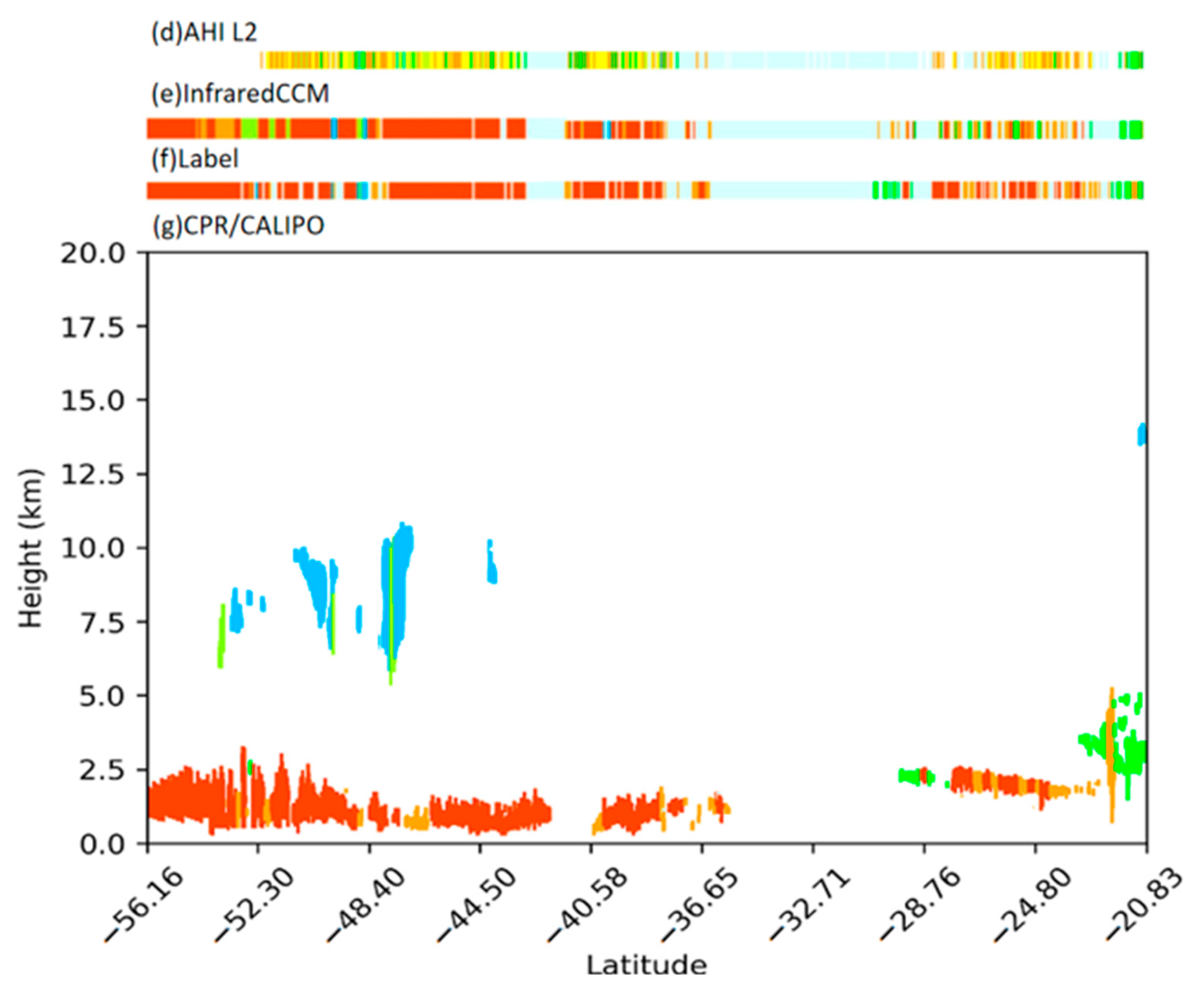
On 15 May 2019, at 04:20 UTC, a cloud map covering southeastern Australia and the South Pacific Ocean was classified using the AInfraredCCM. The data corresponding to the CPR/CALIOP orbit are visually depicted in Figure 8a. The brightness temperature data collected from the 10.4 μm channel of the CPR/CALIOP orbit are displayed in Figure 8b. The AInfraredCCM classification results for this specific region are presented in Figure 8c. The radar track for this scenario extends from the lower-right corner to the upper-left corner of the cloud map, encompassing both daytime and nighttime hours. In this case, the CLTYPE encompasses both daytime and nighttime data, with data in the latitude range from −52.45°S to −56.56°S representing the nighttime region, as depicted in Figure 8d. As part of this comprehensive study, nighttime data, in addition to daytime data, underwent cloud classification. The classification results (Figure 8e) exhibit a significant degree of alignment with the single-layer cloud data (Figure 8f) obtained from the 2B-CLDCLASS-LIDAR. Figure 8f illustrates the outcomes of the combined cloud products of the CPR/CALIOP and Himawari-8 data. Figure 8g provides an insight into the vertical profile of the cloud types along the orbit for CPR/CALIOP.

3.4. Effects of Different Seasons on Cloud Classification

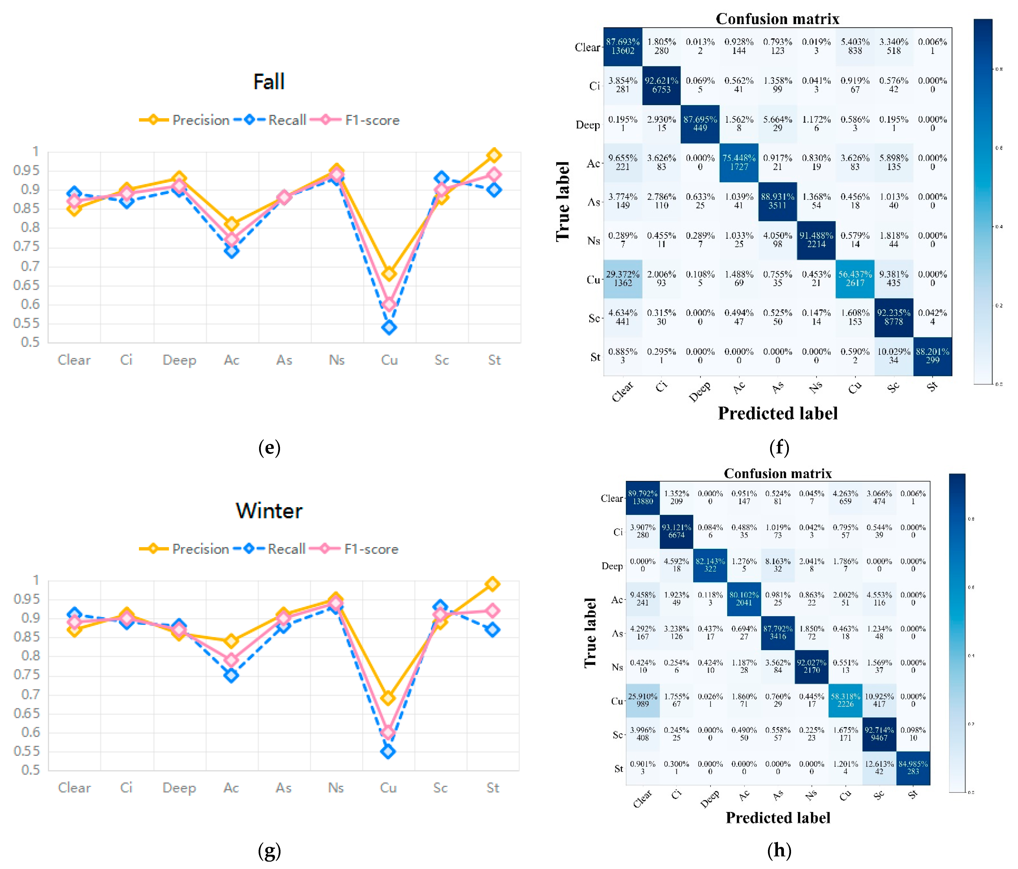
The model was evaluated across all four seasons to determine its suitability. Table 12 presents the performance of AInfraredCCM in different seasons. Figure 9 shows the confusion matrices for the four seasons. The test dataset incorporates data from the four seasons and includes samples from daytime and nighttime observations as well as diverse subsurface information. During spring, summer, autumn, and winter, the overall accuracy was consistently >85% (86.61%, 85.60%, 85.87%, and 87.27% for spring, summer, autumn, and winter, respectively), which is consistent with the overall accuracy of the model. Ci, Dc, Ns, and St exhibited accuracies greater than 90%, coupled with recall and F1-scores of approximately 0.9. However, the classification of Cu remains challenging. Based on the characteristics of Cu, in subsequent experiments, we divided it into continuous and fragmented forms to improve the detection rate of Cu.
Figure 10 shows a comparative analysis of the results for all four seasons, with individual cases (a)–(d) corresponding to spring, summer, autumn, and winter, respectively. The three columns represent the brightness temperature for each case and the classification results of the AInfraredCCM and the CLTYPE. In general, the brightness temperature of a cloud is inversely proportional to its altitude, with lower brightness temperatures indicating higher cloud cover.
Taking the spring scenario (a) as an example, the first image is a brightness temperature map captured on 15 May 2019 at 02:50 UTC. In this figure, the AInfraredCCM effectively classifies the entire cloud image into regions with lower brightness temperature values. However, CLTYPE struggles to identify nighttime areas. In the summer scenario (b) taken at the typhoon center at UTC 05:00 on 5 August 2017, the CLTYPE identified Ci and Dc within the core of the typhoon but encountered difficulties in distinguishing these clouds from clear skies over most of the region. This study is able to finely classify clouds based on their brightness and temperature characteristics. It also categorized fill areas in CLTYPE, thereby enhancing the coherence of the classification results. Owing to the complex cloud composition during typhoons, the classification results of AInfraredCCM are consistent with the actual conditions. In contrast, the CLTYPE exhibited inaccuracies such as mislabeling as Ac in autumn (c). Similarly, the winter scenario (d) resulted in Cu being erroneously classified as clear, with many small cloud structures being misclassified. This study employed a pixel-level cloud classification method that facilitated the identification of more fragmented clouds and cloud pixels that resemble clear skies.

4. Discussion

This study utilized Himawari-8 satellite infrared data and CPR/CALIOP cloud products for conducting comprehensive research on all-day cloud classification. The input features included latitude, longitude, brightness temperature, and brightness temperature difference data derived from Himawari-8. Cloud type labels were extracted from the CloudSat/CALIOP joint secondary product 2B-CLDCLASS-LIDAR. Following this, a cloud classification model was developed to handle all-day observations by leveraging satellite detection. Five machine learning models were employed for model development. The results highlight the superior performance of the AInfraredCCM based on the XGBoost model compared to that of the other models. It achieved impressive overall accuracy, precision, recall, and F1 scores of 86.22%, 0.88, 0.84, and 0.86, respectively.
The AInfraredCCM surpassed many previous models in terms of overall accuracy and cloud classification diversity (Table 9). Unlike previous studies that primarily focused on daytime data due to limited nighttime cloud product data, this study included both daytime and nighttime data. The model performed well at night, yielding an overall classification accuracy of 91.45%. Previous studies on nighttime cloud classification often had a limited range of cloud types. In this study, satellite data were categorized into nine types—clear, Ci, Dc, Ac, As, Ns, St, Sc, and Cu. Compared with other nighttime classification models, this model achieved classification of a broader range of cloud types while maintaining a good overall classification performance. However, due to the limited amount of nighttime data, it may result in a more favorable classification performance. In future research, it is advisable to increase the volume of nighttime data. Through the AInfraredCCM, continuous cloud classification was realized throughout the day with a time resolution of up to 10 min. These high-resolution and continuous cloud classification results provide a richer dataset for exploring various cloud parameters and support all-day meteorological monitoring.
After conducting a comparative and analytical evaluation of the classification results across all-day, daytime, nighttime, and four-season scenarios, it was evident that the classification performance for Cu clouds was relatively subpar. The confusion matrix (Figure 4, Figure 7 and Figure 9) clearly depicts that Cu clouds are predominantly misclassified as clear skies and Sc. This phenomenon is closely related to the developmental stages of Cu. Cu clouds were classified into two types: fragmented and continuous Cu. Fragmented Cu are usually small, which makes their detection using satellite observations challenging. These clouds are easily dispersed by wind and have a short lifespan. Consequently, satellite-based systems may mistakenly identify clear skies as broken Cu clouds. Additionally, Cu clouds, as a convective system forming in the lower atmosphere, can transition into Sc clouds. Cu exhibited distinct characteristics when the convection intensified. If their convection development is suppressed, then Cu clouds may transform into Sc, leading to frequent misidentifications between the two cloud types.
There are some limitations that need to be further investigated. First, the cloud type labels used in this research were derived from the 2B-CLDCLASS-LiDAR product, which is based on data from CPR/CALIOP. During the label screening process, only pixels with a single layer of clouds were selected for comparison with the CLTYPE. Moreover, the majority principle was employed for cloud type screening during filtering labels. It is important to note that this screening method may result in the omission of certain data with limited feature information, particularly in the case of fragmented Cu and optically thin Ci. To improve the quality of the dataset, more refined label-generation techniques should be explored in future studies. Second, errors can arise when observing the same object using the Himawari-8 and CloudSat satellites from different observation positions. Spatiotemporal matching errors may be more pronounced, especially in regions with large observation angles [43,44]. Therefore, error correction is vital. In future research, the cloud positions in the AHI data could be computed using cloud information, including longitude, latitude, and cloud top height, collected by CALIPSO satellites. The corrected cloud positions can then be used to create a more accurate dataset [34,45].

5. Conclusions

This study describes an algorithm for all-day cloud classification, referred to as AInfraredCCM, which is based on machine learning and utilizes Himawari-8 data. AHI and CPR/CALIOP data collected in November 2018, January 2019, March 2019, and June–July 2019 were used to develop the algorithm. After preprocessing, the data were randomly divided according to a ratio of 9:1. Of the data, 90% were allocated to the training and validation datasets for algorithm development, while the remaining 10% were reserved for testing. The predictors employed in this algorithm include 10 IR channels, 5 BTDs channels, and latitude and longitude information. The conclusions of this study are detailed here:
(1)
The overall accuracy, precision, recall, and F1-score of AInfraredCCM cloud classification were 86.22%, 0.88, 0.84, and 0.86, respectively. Notably, the here-proposed model outperformed the other models selected for this study (Table 8) and those proposed by other researchers (Table 9). These results indicate that it is an efficient all-day cloud classification method.
(2)
The model performed well when used for all-day cloud classification or when used separately for daytime and nighttime classification, which suggests that the AInfraredCCM provides continuous data for cloud classification research throughout the day.
(3)
The model was applied to both day and night scenarios as well as to four seasons and produced good classification results. In addition to Cu, this study demonstrated efficacy in classifying other cloud types. More emphasis should be laid on Cu in future studies.

Supplementary Materials

The following supporting information can be downloaded at: https://www.mdpi.com/article/10.3390/rs15245630/s1, Figures S1–S130 represent the thematic map of Himawari-8’s official cloud-type products and the classification results generated by the AInfraredCCM at UTC 4:00 for 130 days.

Author Contributions

The authors’ contributions are as follows: conceptualization, methodology, validation, formal analysis, and data curation, Y.F. and W.Z.; writing—original draft preparation, Y.F. and X.M.; writing—review and editing, all authors; supervision, Z.H. and Q.L.; funding acquisition, W.Z. and X.M.; and project administration, X.G. and T.Y. All authors have read and agreed to the published version of the manuscript.

Funding

The Major Project of High-Resolution Earth Observation System, No. 30-Y60B01-9003-22/23 and No. 30-Y30F06-9003-20/22; North China Institute of Aerospace Engineering Foundation of Doctoral Research, BKY-2021-31; Science and Technology Research Projects of Higher Education Institutions in Hebei Province, ZD2021303; Hebei Province Graduate Student Innovation Ability Training Funding Project, No. CXZZSS2023166, North China Institute of Aerospace Engineering’s University-level Innovation Project, No. YKY-2022-58.

Data Availability Statement

The data in this article can be found online at https://github.com/tpmao/cloud-classification-data, accessed on 13 October 2023.

Conflicts of Interest

The authors declare no conflict of interest.

Appendix A

Table A1 shows 130 images of the whole area of Himawari-8 from 2018 to 2019, which is used to compare and verify the model classification results with Himawari-8 CLTYPE in Section 3.2. The data are categorized into four folders based on the seasons.
Table A1. The statistics of AInfraredCCM classification results for the four seasons and corresponding CLTYPE of Himawari-8.
SeasonNo.Data IDNo.Data ID
Spring120190301_04001720190317_0400
220190302_04001820190318_0400
320190303_04001920190319_0400
420190304_04002020190320_0400
520190305_04002120190321_0400
620190306_04002220190322_0400
720190307_04002320190323_0400
820190308_04002420190324_0400
920190309_04002520190325_0400
1020190310_04002620190326_0400
1120190311_04002720190327_0400
1220190312_04002820190328_0400
1320190313_04002920190329_0400
1420190314_04003020190330_0400
1520190315_04003120190331_0400
1620190316_0400
Summer3220190601_04005120190620_0400
3320190602_04005220190622_0400
3420190603_04005320190623_0400
3520190604_04005420190624_0400
3620190605_04005520190625_0400
3720190606_04005620190626_0400
3820190607_04005720190627_0400
3920190608_04005820190628_0400
4020190609_04005920190630_0400
4120190610_04006020190701_0400
4220190611_04006120190702_0400
4320190612_04006220190703_0400
4420190613_04006320190704_0400
4520190614_04006420190705_0400
4620190615_04006520190706_0400
4720190616_04006620190707_0400
4820190617_04006720190708_0400
4920190618_04006820190709_0400
5020190619_04006920190710_0400
Autumn7020181101_04008520181116_0400
7120181102_04008620181117_0400
7220181103_04008720181118_0400
7320181104_04008820181119_0400
7420181105_04008920181120_0400
7520181106_04009020181121_0400
7620181107_04009120181122_0400
7720181108_04009220181123_0400
7820181109_04009320181124_0400
7920181110_04009420181125_0400
8020181111_04009520181126_0400
8120181112_04009620181127_0400
8220181113_04009720181128_0400
8320181114_04009820181129_0400
8420181115_04009920181130_0400
Winter10020190601_040011620190617_0400
10120190602_040011720190618_0400
10220190603_040011820190619_0400
10320190604_040011920190620_0400
10420190605_040012020190621_0400
10520190606_040012120190622_0400
10620190607_040012220190623_0400
10720190608_040012320190624_0400
10820190609_040012420190625_0400
10920190610_040012520190626_0400
11020190611_040012620190627_0400
11120190612_040012720190628_0400
11220190613_040012820190629_0400
11320190614_040012920190630_0400
11420190615_040013020190631_0400
11520190616_0400

References

  1. Tapakis, R.; Charalambides, A.G. Equipment and methodologies for cloud detection and classification: A review. Sol. Energy 2013, 95, 392–430. [Google Scholar] [CrossRef]
  2. Stubenrauch, C.J.; Rossow, W.B.; Kinne, S.; Ackerman, S.; Cesana, G.; Chepfer, H.; Di Girolamo, L.; Getzewich, B.; Guignard, A.; Heidinger, A.; et al. Assessment of Global Cloud Datasets from Satellites: Project and Database Initiated by the GEWEX Radiation Panel. Bull. Am. Meteorol. Soc. Bull. Am. Meteorol. Soc. 2013, 94, 1031–1049. [Google Scholar] [CrossRef]
  3. Rossow, W.B.; Mosher, F.; Kinsella, E.; Arking, A.; Desbois, M.; Harrison, E.; Minnis, P.; Ruprecht, E.; Seze, G.; Simmer, C. ISCCP cloud algorithm intercomparison. J. Appl. Meteorol. Clim. 1985, 24, 877–903. [Google Scholar] [CrossRef]
  4. Zhuang, Z.H.; Wang, M.; Wang, K.; Li, S.; Wu, J. Research progress of ground-based cloud classification technology based on deep learning. J. Nanjing Univ. Inf. Sci. Technol. (Nat. Sci. Ed.) 2022, 14, 566–578. [Google Scholar] [CrossRef]
  5. Zhao, C.; Garrett, T.J. Effects of Arctic haze on surface cloud radiative forcing. Geophys. Res. Lett. 2015, 42, 557–564. [Google Scholar] [CrossRef]
  6. Liu, Y.; Xia, J.; Shi, C.-X.; Hong, Y. An Improved Cloud Classification Algorithm for China’s FY-2C Multi-Channel Images Using Artificial Neural Network. Sensors 2009, 9, 5558–5579. [Google Scholar] [CrossRef]
  7. Chen, D.; Guo, J.; Wang, H.; Li, J.; Min, M.; Zhao, W.; Yao, D. The Cloud Top Distribution and Diurnal Variation of Clouds Over East Asia: Preliminary Results From Advanced Himawari Imager. J. Geophys. Res. Atmos. 2018, 123, 3724–3739. [Google Scholar] [CrossRef]
  8. Astafurov, V.G.; Skorokhodov, A.V. Using the results of cloudclassification based on satellite data for solving climatological andmeteorological problems. Russ. Meteorol. Hydrol. 2021, 46, 839–848. [Google Scholar] [CrossRef]
  9. Toğaçar, M.; Ergen, B. Classification of cloud images by using super resolution, semantic segmentation approaches and binary sailfish optimization method with deep learning model. Comput. Electron. Agric. 2022, 193, 106724. [Google Scholar] [CrossRef]
  10. Zhang, C.; Zhuge, X.; Yu, F. Development of a high spatiotemporal resolution cloud-type classification approach using Himawari-8 and CloudSat. Int. J. Remote Sens. 2019, 40, 6464–6481. [Google Scholar] [CrossRef]
  11. Wohlfarth, K.; Schröer, C.; Klaß, M.; Hakenes, S.; Venhaus, M.; Kauffmann, S.; Wilhelm, T.; Wohler, C. Dense Cloud Classification on Multispectral Satellite Imagery. In Proceedings of the 2018 10th IAPR Workshop on Pattern Recognition in Remote Sensing (PRRS), Beijing, China, 19–20 August 2018; pp. 1–6. [Google Scholar] [CrossRef]
  12. Yu, Z.; Ma, S.; Han, D.; Li, G.; Gao, D.; Yan, W. A cloud classification method based on random forest for FY-4A. Int. J. Remote Sens. 2021, 42, 3353–3379. [Google Scholar] [CrossRef]
  13. Cai, K.; Wang, H. Cloud classification of satellite image based on convolutional neural networks. In Proceedings of the 2017 8th IEEE International Conference on Software Engineering and Service Science (ICSESS), Beijing, China, 24–26 November 2017; pp. 874–877. [Google Scholar] [CrossRef]
  14. Afzali Gorooh, V.; Kalia, S.; Nguyen, P.; Hsu, K.-l.; Sorooshian, S.; Ganguly, S.; Nemani, R.R. Deep Neural Network Cloud-Type Classification (DeepCTC) Model and Its Application in Evaluating PERSIANN-CCS. Remote Sens. 2020, 12, 316. [Google Scholar] [CrossRef]
  15. Olesen, F.-S.; Grassl, H. Cloud detection and classification over oceans at night with NOAA-7. Int. J. Remote Sens. 1985, 6, 1435–1444. [Google Scholar] [CrossRef]
  16. Tan, Z.; Liu, C.; Ma, S.; Wang, X.; Shang, J.; Wang, J.; Ai, W.; Yan, W. Detecting Multilayer Clouds From the Geostationary Advanced Himawari Imager Using Machine Learning Techniques. IEEE Trans. Geosci. Remote Sens. 2022, 60, 4103112. [Google Scholar] [CrossRef]
  17. Li, W.; Zhang, F.; Lin, H.; Chen, X.; Li, J.; Han, W. Cloud Detection and Classification Algorithms for Himawari-8 Imager Measurements Based on Deep Learning. IEEE Trans. Geosci. Remote Sens. 2022, 60, 4107117. [Google Scholar] [CrossRef]
  18. Letu, H.; Nagao, T.M.; Nakajima, T.Y.; Riedi, J.; Ishimoto, H.; Baran, A.J.; Shang, H.; Sekiguchi, M.; Kikuchi, M. Ice Cloud Properties from Himawari-8/AHI Next-Generation Geostationary Satellite: Capability of the AHI to Monitor the DC Cloud Generation Process. IEEE Trans. Geosci. Remote Sens. 2019, 57, 3229–3239. [Google Scholar] [CrossRef]
  19. Min, M.; Bai, C.; Guo, J.; Sun, F.; Liu, C.; Wang, F.; Xu, H.; Tang, S.; Li, B.; Di, D.; et al. Estimating Summertime Precipitation from Himawari-8 and Global Forecast System Based on Machine Learning. IEEE Trans. Geosci. Remote Sens. 2019, 57, 2557–2570. [Google Scholar] [CrossRef]
  20. Min, M.; Wu, C.; Li, C.; Liu, H.; Xu, N.; Wu, X.; Chen, L.; Wang, F.; Sun, F.; Qin, D.; et al. Developing the science product algorithm testbed for Chinese next-generation geostationary meteorological satellites: Fengyun-4 series. J. Meteorol. Res. 2017, 31, 708–719. [Google Scholar] [CrossRef]
  21. Bessho, K.; Date, K.; Hayashi, M.; Ikeda, A.; Imai, T.; Inoue, H.; Kumagai, Y.; Miyakawa, T.; Murata, H.; Ohno, T.; et al. An Introduction to Himawari-8/9—Japan’s New-Generation Geostationary Meteorological Satellites. J. Meteor. Soc. Jpn. 2016, 94, 151–183. [Google Scholar] [CrossRef]
  22. Stephens, G.; Winker, D.; Pelon, J.; Trepte, C.; Vane, D.; Yuhas, C.; L’Ecuyer, T.; Lebsock, M. CloudSat and CALIPSO within the A-Train: Ten Years of Actively Observing the Earth System. Bull. Am. Meteorol. Soc. Bull. Am. Meteorol. Soc. 2018, 99, 569–581. [Google Scholar] [CrossRef]
  23. Winker, D.M.; Vaughan, M.A.; Omar, A.; Hu, Y.; Powell, K.A.; Liu, Z.; Hunt, W.H.; Young, S.A. Overview of the CALIPSO Mission and CALIOP Data Processing Algorithms. J. Atmos. Ocean. Technol. 2009, 26, 2310–2323. [Google Scholar] [CrossRef]
  24. Sassen, K.; Wang, Z.; Liu, D. Global distribution of cirrus clouds from CloudSat/Cloud-Aerosol Lidar and Infrared Pathfinder Satellite Observations (CALIPSO) measurements. J. Geophys. Res. 2008, 113, D00A12. [Google Scholar] [CrossRef]
  25. Stephens, G.L.; Vane, D.G.; Boain, R.J.; Mace, G.G.; Sassen, K.; Wang, Z.; Illingworth, A.J.; O’Connor, E.J.; Rossow, W.B.; Durden, S.L.; et al. THE CLOUDSAT MISSION AND THE A-TRAIN: A New Dimension of Space-Based Observations of Clouds and Precipitation. Bull. Am. Meteorol. Soc. 2002, 83, 1771–1790. [Google Scholar] [CrossRef]
  26. Unglaub, C.; Block, K.; Mülmenstädt, J.; Sourdeval, O.; Quaas, J. A new classification of satellite-derived liquid water cloud regimes at cloud scale. Atmos. Chem. Phys. 2020, 20, 2407–2418. [Google Scholar] [CrossRef]
  27. Wang, Z. CloudSat 2B-CLDCLASS-LIDAR Product Process Description and Interface Control Document; Process Description and Interface Control Document (PDICD) P1_R05; NASA: Washington, DC, USA, 2019; Volume 33.
  28. Zhang, A.; Fu, Y. Life Cycle Effects on the Vertical Structure of Precipitation in East China Measured by Himawari-8 and GPM DPR. Mon. Weather Rev. 2018, 146, 2183–2199. [Google Scholar] [CrossRef]
  29. Strabala, K.I.; Ackerman, S.A.; Menzel, W.P. Cloud Properties inferred from 8–12 µm Data. J. Appl. Meteor. Climatol. 1994, 33, 212–229. [Google Scholar] [CrossRef]
  30. Chen, S.; Cheng, C.; Zhang, X.; Su, L.; Tong, B.; Dong, C.; Wang, F.; Chen, B.; Chen, W.; Liu, D. Construction of Nighttime Cloud Layer Height and Classification of Cloud Types. Remote Sens. 2020, 12, 668. [Google Scholar] [CrossRef]
  31. Yue, Q.; Fetzer, E.J.; Kahn, B.H.; Wong, S.; Manipon, G.; Guillaume, A.; Wilson, B. Cloud-State-Dependent Sampling in AIRS Observations Based on CloudSat Cloud Classification. J. Clim. 2013, 26, 8357–8377. [Google Scholar] [CrossRef]
  32. Berry, E.; Mace, G.G. Cloud properties and radiative effects of the Asian summer monsoon derived from A-Train data. J. Geophys. Res. Atmos. 2014, 119, 9492–9508. [Google Scholar] [CrossRef]
  33. Behrangi, A.; Kubar, T.; Lambrigtsen, B. Phenomenological Description of Tropical Clouds Using CloudSat Cloud Classification. Mon. Weather Rev. 2012, 140, 3235–3249. [Google Scholar] [CrossRef]
  34. Yang, Y.; Sun, W.; Chi, Y.; Yan, X.; Fan, H.; Yang, X.; Ma, Z.; Wang, Q.; Zhao, C. Machine learning-based retrieval of day and night cloud macrophysical parameters over East Asia using Himawari-8 data. Remote Sens. Environ. 2022, 273, 112971. [Google Scholar] [CrossRef]
  35. Liu, C.; Yang, S.; Di, D.; Yang, Y.; Zhou, C.; Hu, X.; Sohn, B.-J. A Machine Learning-based Cloud Detection Algorithm for the Himawari-8 Spectral Image. Adv. Atmos. Sci. 2022, 39, 1994–2007. [Google Scholar] [CrossRef]
  36. Tan, Y.; Zhang, W.; Yang, X.; Liu, Q.; Mi, X.; Li, J.; Yang, J.; Gu, X. Cloud and Cloud Shadow Detection of GF-1 Images Based on the Swin-UNet Method. Atmosphere 2023, 14, 1669. [Google Scholar] [CrossRef]
  37. Fan, X.; Kong, J.L.; Zhong, Y.L.; Jiang, Y.Z.; Zhang, J.Y. Cloud Detection of Remote Sensing Images based on XGBoost Algorithm. Remote Sens. Technol. Appl. 2023, 38, 156–162. [Google Scholar]
  38. Mommert, M. Cloud Identification from All-sky Camera Data with Machine Learning. Astron. J. 2020, 159, 178. [Google Scholar] [CrossRef]
  39. Jiang, Y.; Cheng, W.; Gao, F.; Zhang, S.; Wang, S.; Liu, C.; Liu, J. A Cloud Classification Method Based on a Convolutional Neural Network for FY-4A Satellites. Remote Sens. 2022, 14, 2314. [Google Scholar] [CrossRef]
  40. Wang, B.; Zhou, M.; Cheng, W.; Chen, Y.; Sheng, Q.; Li, J.; Wang, L. An Efficient Cloud Classification Method Based on a Densely Connected Hybrid Convolutional Network for FY-4A. Remote Sens. 2023, 15, 2673. [Google Scholar] [CrossRef]
  41. Wang, Y.; Hu, C.; Ding, Z.; Wang, Z.; Tang, X. All-Day Cloud Classification via a Random Forest Algorithm Based on Satellite Data from CloudSat and Himawari-8. Atmosphere 2023, 14, 1410. [Google Scholar] [CrossRef]
  42. Cermak, J.; Bendix, J. A novel approach to fog/low stratus detection using Meteosat 8 data. Atmos. Res. 2008, 87, 279–292. [Google Scholar] [CrossRef]
  43. Guo, Q.; Feng, X.; Yang, C.; Chen, B. Improved Spatial Collocation and Parallax Correction Approaches for Calibration Accuracy Validation of Thermal Emissive Band on Geostationary Platform. IEEE Trans. Geosci. Remote Sens. 2018, 56, 2647–2663. [Google Scholar] [CrossRef]
  44. Kim, H.-W.; Yeom, J.-M.; Shin, D.; Choi, S.; Han, K.-S.; Roujean, J.-L. An assessment of thin cloud detection by applying bidirectional reflectance distribution function model-based background surface reflectance using Geostationary Ocean Color Imager (GOCI): A case study for South Korea. J. Geophys. Res. Atmos. 2017, 122, 8153–8172. [Google Scholar] [CrossRef]
  45. Vicente, G.A.; Davenport, J.C.; Scofield, R.A. The role of orographic and parallax corrections on real time high resolution satellite rainfall rate distribution. Int. J. Remote Sens. 2002, 23, 221–230. [Google Scholar] [CrossRef]
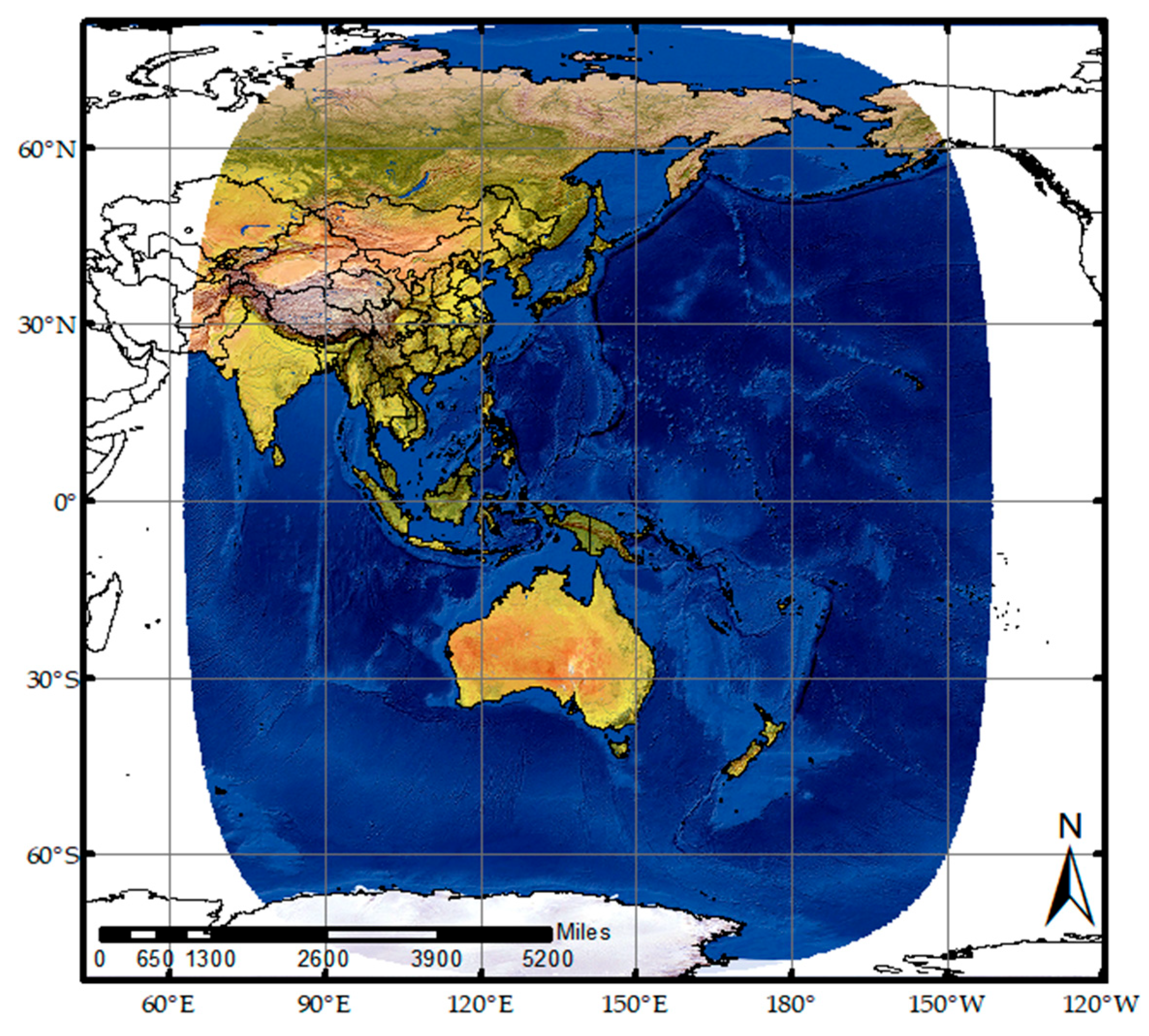
Figure 1. Illustration of the observation area of the Himawari-8 satellite.
Remotesensing 15 05630 g001
Figure 2. Cloud data for 10 channels of AHI.
Remotesensing 15 05630 g002
Figure 3. General flow diagram.
Remotesensing 15 05630 g003
Figure 4. Confusion matrix of the AInfraredCCM.
Remotesensing 15 05630 g004
Figure 5. Classification performance graphs of different models. (ae) Graphs of the precision, recall, and F1-scores of classification results of 5 models in different cloud types.
Remotesensing 15 05630 g005
Figure 6. Classification results of different models at 05:00 UTC on June 29, 2019. (a) Visible data, (b) thermal infrared data, (c) the brightness temperature map; (dh) sequentially present the classification results of GradientBoost, LightGBM, RF, AdaBoost, and AInfraredCCM, respectively.
Remotesensing 15 05630 g006aRemotesensing 15 05630 g006b
Figure 7. Evaluation of classification metrics of the AInfraredCCM for daytime/nighttime. (a,b) Bar graphs of precision, recall, and F1-score of different types of cloud classification results; (c,d) confusion matrix of different types of cloud classification in daytime and nighttime.
Remotesensing 15 05630 g007
Figure 8. Plot of classification results at 04:20 UTC on May 15, 2019. (a) RGB; (b) bright temperature; (c) AInfraredCCM results; (d,e) CLTYPE, AInfraredCCM results, and label; (f) the combined cloud products of the CPR/CALIOP and Himawari-8 data; (g) vertical profiles of the cloud types along the orbit of the CPR/CALIOP.
Remotesensing 15 05630 g008aRemotesensing 15 05630 g008b
Figure 9. Evaluation metrics of the model across 4 seasons; (ah) are the line graphs and confusion matrix of precision, recall, and F1-score in 4 seasons.
Remotesensing 15 05630 g009aRemotesensing 15 05630 g009b
Figure 10. Bright temperatures (K), AInfraredCCM classification results, and Himawari-8 CLTYPE for different seasons. (ad) Cloud map moments in the following order: 15 May 2019 UTC 02:50; 5 August 2017 UTC 05:00; 10 October 2018 UTC 03:30; and 1 February 2019 UTC 06:40, respectively.
Remotesensing 15 05630 g010
Table 1. Himawari-8 band parameters and applications.
BandsChannel TypeCenter Wavelength (μm)Spatial
Resolution (km)
Main Applications
7Midwave IR3.92Natural disasters, low cloud (fog) observation
8Water vapor6.22Observation of water vapor volume in the upper and middle layers
96.92Observations of water vaporization in the mesosphere
107.32
11Longwave IR8.62Cloud phase identification and SO2 detection
129.62Measurement of total ozone
1310.42Observation of cloud images and cloud top conditions
1411.22Observation of cloud images and sea surface water temperature
1512.42Observation of cloud images and sea surface water temperature
1613.32Measurement of cloud height
Table 2. Cloud type of this study.
Cloud LabelLabel of CPR/CALIOPLabel of CLTYPEName of Cloud
00 (Clear)0 (Clear)Clear
11 (Ci)1, 2 (Ci, Cs)Ci (Ci, Cs)
28 (Dc)3 (Dc)Dc
33 (Ac)4 (Ac)Ac
42 (As)5 (As)As
57 (Ns)6 (Ns)Ns
66 (Cu)7 (Cu)Cu
75 (Sc)8 (Sc)Sc
84 (St)9 (St)St
Table 3. Information of dataset.
DimensionNumberVariables
PredictorBTs (10)BT (3.9 μm), BT (6.2 μm), BT (6.9 μm), BT (7.3 μm), BT (8.6 μm), BT (9.6 μm), BT (10.4 μm), BT (11.2 μm), BT (12.4 μm), and BT (13.3 μm)
BTDs (5)BTD (11.2–7.3 μm), BTD (3.9–11.2 μm), BTD (11.2–12.4 μm),
BTD (12.4–10.4 μm), and BTD (7.3–10.4 μm)
Auxiliary data (2)Latitude and Longitude
Prediction1Cloud label from 2B-CLDCLASS-LIDAR and CLTYPE
Table 4. Classification results of the model on dataset C.
Number of Ever CategoryTotal Number
Number of category A cloudsNumber of category B clouds
Model classification resultNumber of category A cloudsTAFBT1
Number of category B cloudsFATBT2
Total number ASBST
Table 5. Parameters of the AInfraredCCM.
ParameterMeaningValue
n_estimatorsNumber of trees204
learning_rateMagnitude of the iterative model update0.2122
max_depthMaximum tree depth26
min_child_weightMinimum number of samples required in a leaf node3
Table 6. Precision, recall, and F1-score of the AInfraredCCM.
Cloud TypePrecisionRecallF1-Score
Clear0.850.890.87
Ci0.900.880.89
Dc0.930.870.90
Ac0.820.740.78
As0.890.880.89
Ns0.950.930.94
Cu0.680.570.60
Sc0.880.930.91
St0.980.900.94
Table 7. Optimal parameter combinations for the model.
AlgorithmParameted Range
Random Forest1. max_depth = 73
2. n_estimators = 280
LightGBM1. learning_rate = 0.095
2. max_depth = 22
3. n_estimators = 252
4. num_leaves = 35
AdaBoost1. learning_rate = 0.4224
2. max_depth = 74
3. n_estimators = 458
4. min_samples_leaf = 1
GradientBoost1. learning_rate = 0.4749
2. max_depth = 37
3. n_estimators = 10
Table 8. Evaluation for different models.
AlgorithmAccuracyPrecisionRecallF1-Score
Random Forest82.53%0.830.760.79
LightGBM74.60%0.700.640.66
GradientBoost80.96%0.780.770.78
AdaBoost85.83%0.870.830.85
AInfraredCCM86.22%0.880.840.86
Table 9. Cloud classification model statistical table.
ModelCategoryFeatureTimeOASampleReference
RFDc, Ns, Cu, Sc, St, Ac, As, Ci, and multiREF and BT of 13 channels, cloud top height, cloud optical
thickness, cloud effective radius
Day0.67272414Yu et al. (2021) [12]
BPClear, low cloud, middle cloud, thick cirrus clouds, thin cirrus cloud, deep convectiveIR1 (10.3–11.3), IR2 (11.5–12.5), WV (6.3–7.6), IR1-IR2, IR1-WV, IR2-WVDay0.862449Zhang et al. (2012) [39]
CNNClear, Ci, Ac, As, Sc, Dc, Ns, CuAll channel of FY-4ADay0.9515780Wang et al. (2023) [40]
RFClear, low cloud, middle cloud, thin cloud, thick cloud, multilayer cloud, cumulonimbusR (0.64), R (1.6), BT (11.2 μm), BTD (11.2–3.9 μm), BTD (11.2–7.3 μm), BTD (11.2–8.6 μm), BTD (11.2–12.3 μm)Day0.88127192Wang et al. (2023) [41]
RFClear, low cloud, middle cloud, thin cloud, thick cloud, multilayer cloud, cumulonimbusBT (11.2 μm), BTD (11.2–3.9 μm), BTD (11.2–7.3 μm), BTD (11.2–8.6 μm), BTD (11.2–12.3 μm)Night0.7972934Wang et al. (2023) [41]
RFClear, single, multiBT (3.9 um), BT (7.3 m), BT (8.6 μm),
BT (11.2 μm), BT (12.4 μm),
BTD (3.9–11.2 μm), BTD (8.6–11.2 μm), BTD (11.2–12.4 μm), latitude, longitude
Day and night0.7912553889Tan et al. (2022) [16]
DNNClear, single-ice, single-mixed, single-water, multiBT (3.9–13.3 μm), cosine of satellite zenith angle, simulated clear-sky radiancesDay and night0.811114591Li et al. (2022) [17]
AInfraredCCMClear, Ci, Dc, Ac, As, Ns, Cu, Sc, StBT (3.9–13.3 μm), BTD (11.2–9.6 μm),
BTD (3.9–11.2 μm), BTD (11.2–12.4 μm), BTD (12.4–10.4 μm), BTD (7.3–10.4 μm), latitude, longitude
Day and night0.861314275This study
Table 10. Accuracy rate of Himawari-8 CLTYPE and AInfraredCCM.
Himawari-8 CLTYPEAInfraredCCM
Full area0.480.86
Cloudy area0.360.87
Clear sky0.770.85
Table 11. Cloud classification results of the AInfraredCCM for daytime and nighttime.
TimeCloud TypeClearCiDcAcAsNsCuScSt
Accuracy = 85.82%
DaytimePrecision0.850.900.920.820.890.950.680.890.98
Recall0.890.880.860.720.880.930.540.920.90
F1-score0.870.890.890.770.880.940.600.910.94
Accuracy = 91.45%
NighttimePrecision0.900.920.990.870.920.960.770.930.97
Recall0.900.910.920.850.930.970.560.960.96
F1-score0.900.910.950.860.930.960.650.940.96
Table 12. Results of the four seasonal classifications.
SeasonCloud TypeClearCiDcAcAsNsCuScSt
Accuracy = 86.61%
SpringPrecision0.850.900.930.830.900.960.690.900.97
Recall0.900.870.870.750.870.940.560.930.90
F1-score0.880.880.900.790.890.950.620.920.93
Accuracy = 85.60%
SummerPrecision0.840.910.950.820.870.950.660.880.97
Recall0.880.890.890.740.880.930.500.920.93
F1-score0.860.900.920.780.880.940.570.900.95
Accuracy = 85.87%
AutumnPrecision0.850.900.930.810.880.950.680.880.99
Recall0.890.870.900.740.880.930.540.930.90
F1-score0.870.890.910.770.880.940.600.900.94
Accuracy = 87.27%
WinterPrecision0.870.910.860.840.910.950.690.890.99
Recall0.910.890.880.750.880.930.550.930.87
F1-score0.890.900.870.790.900.940.600.910.92
Disclaimer/Publisher’s Note: The statements, opinions and data contained in all publications are solely those of the individual author(s) and contributor(s) and not of MDPI and/or the editor(s). MDPI and/or the editor(s) disclaim responsibility for any injury to people or property resulting from any ideas, methods, instructions or products referred to in the content.