Abstract
Greenhouse gases such as CH4 generated by forest fires have a significant impact on atmospheric methane concentrations and terrestrial vegetation methane budgets. Verification in conjunction with “top-down” satellite remote sensing observation has become a vital way to verify biomass-burning emission inventories and accurately assess greenhouse gases while looking into the limitations in reliability and quantification of existing “bottom-up” biomass-burning emission inventories. Therefore, we considered boreal forest fire regions as an example while combining five biomass-burning emission inventories and CH4 indicators of atmospheric concentration satellite observation data. By introducing numerical comparison, correlation analysis and trend consistency analysis methods, we explained the lag effect between emissions and atmospheric concentration changes and evaluated a more reliable emission inventory using time series similarity measurement methods. The results indicated that total methane emissions from five biomass-burning emission inventories differed by a factor of 2.9 in our study area, ranging from 2.02 to 5.84 Tg for methane. The time trends of the five inventories showed good consistency, with the Quick Fire Emissions Dataset version 2.5 (QFED2.5) having a higher correlation coefficient (above 0.8) with the other four datasets. By comparing the consistency between the inventories and satellite data, a lagging effect was found to be present between the changes in atmospheric concentration and gas emissions caused by forest fires on a seasonal scale. After eliminating lagging effects and combining time series similarity measures, the QFED2.5 (Euclidean distance = 0.14) was found to have the highest similarity to satellite data. In contrast, Global Fire Emissions Database version 4.1 with small fires (GFED4.1s) and Global Fire Assimilation System version 1.2 (GFAS1.2) had larger Euclidean distances of 0.52 and 0.4, respectively, which meant that they had lower similarity to satellite data. Therefore, QFED2.5 was found to be more reliable while having higher application accuracy compared to the other four datasets in our study area. This study further provided a better understanding of the key role of forest fire emissions in atmospheric CH4 concentrations and offered reference for selecting appropriate biomass burning emission inventory datasets for bottom-up inventory estimation studies.
1. Introduction
Forest fires, one of the main natural disturbances in boreal forests [1,2], are known to have a long duration and wide spatial range and cause significant losses [3]. Boreal forests are located in high latitude areas and cover vast territories, making them ideal places to monitor global climate change [4]. Approximately 5–20 million hectares of forestland in boreal forests are burned out annually [5,6]. Boreal forests accounted for the majority (nearly 70%) of all tree cover losses caused by fires over the past 10 years [7,8]. In 2021, the key areas of global fires mainly included North America, Canada, Siberia and the Far East region. The average area of forest fires in Russia reached 1,679,534 hectares from 2012 to 2021 [8].
The forest fires are accompanied by the emissions of toxic gases and various harmful particles (ex: CH4), making a significant contribution to regional and global carbon emissions. It is estimated that the total global emissions of CO2, CO, and CH4 from forest fires are 3135 Tg C/year, 228 Tg C/year, and 167 Tg C/year, respectively, accounting for 45%, 21%, and 44% of all global source emissions [9]. The highest methane emissions from biomass burning in the northern forest region accounted for 45% of the global methane emissions during the summer of 2010, when forest fires were frequent (https://gml.noaa.gov/ccgg/carbontracker-ch4/ (accessed on 6 July 2023)). When severe forest fires occurred in the 2010 North American Northern Forest Severe Fire Incident, methane emissions accounted for 30% to 45% of the total gas emissions (https://gml.noaa.gov/ccgg/carbontracker-ch4/ (accessed on 6 July 2023)). As one of the main greenhouse gases, methane is more active in the atmosphere than carbon dioxide. Although it has a lower atmospheric concentration than carbon dioxide, it has 84 times higher warming potential within a 20-year scale [10]. The atmospheric concentration of methane is steadily increasing. For example, data from the Japanese Greenhouse Gases Observing Satellite (GOSAT) revealed that the global monthly mean CH4 concentration reached 1873 ppb in March 2023, with a growth rate of 15 ppb year−1 from March 2022 to March 2023 (https://www.gosat.nies.go.jp/recent-global-ch4.html (accessed on 6 July 2023)). Reducing methane emissions can be considered an effective way to quickly mitigate climate change because of methane’s shorter lifetime than CO2 [11]. However, the estimation of methane emissions is influenced by numerous factors (fire area, combustion type, season and wind speed) that make it challenging to accurately quantify the methane released by forest fires [12]. Considering the goal of emission reduction and understanding global climate change as well as the carbon cycle, it is vital to accurately estimate CH4 emissions from regional forest fires [13,14].
The widely used “bottom-up” Global Biomass Burning Emission Inventory (GBBEI) can provide bottom-up, near-surface and near-real-time data sources for estimating CH4 emissions from forest fires [15]. In order to better apply the existing GBBEI to the assessment of air pollutant emissions, existing research used emission comparisons from different inventory data using methods such as time correlation analysis and global chemical transport models (GEOS-Chem) and looked for differences between inventory data [16,17]. However, due to the dynamic characteristics of fire behavior and the input of related combustion parameters [18], GBBEI has discrepancies over spatial and temporal scales [19], making it challenging to estimate the reliability of GBBEI in quantifying fire-induced emissions in global continental regions [16].
Given the limitations of the “bottom-up” GBBEI, the IPCC explicitly proposed the standard of using atmospheric concentration measurements to assist inventory verification through the “IPCC 2006 National Greenhouse Gas Inventory Guidelines 2019 Revision”. It is based on determining atmospheric concentrations by remote sensing measurements and ground base station measurements in combination with the “top-down” (i.e., atmospheric inversion) model to estimate greenhouse gas emissions while verifying and correcting the results of traditional bottom-up national greenhouse gas inventories. With the consistent development of carbon satellite monitoring capabilities and accuracy, a growing number of studies are using atmospheric concentration satellite monitoring data and ground station observation data to verify and correct emission inventories while obtaining more reliable emission inventory products [12,20,21,22]. Regression statistics and fitting analysis methods are mostly used to compare carbon dioxide emissions and concentration information between inventory and satellite data at a large regional scale [20,22]. However, there are many methane emission sources, and we should try our best to eliminate interference from other emission sources (wetlands, permafrost, fuel combustion, etc.) [23,24]. Therefore, we selected forest fires as the main source of interference to reduce the interference from other emissions and reliably assess the accuracy of inventories.
Five commonly used GBBEIs, atmospheric concentration satellite data and ground station observation concentration data were selected in this study. As one of the most active greenhouse gases, methane was selected as our research object. In order to understand the relationship between methane emissions caused by fires in boreal forests and atmospheric concentrations from 2010 to 2020, we used numerical comparison, correlation analysis and trend consistency analysis to quantitatively analyze the consistency and differences between datasets at the regional scale. Furthermore, using satellite data as the measurement standard, we quantitatively explored the similarity between each inventory dataset and satellite data in terms of time trends using the time similarity method. Moreover, based on previous research findings on inventory data, we evaluated a more reliable inventory. With the help of this study, we can better address the rapid growth of greenhouse gas concentrations, implement targeted greenhouse gas emission control policies and provide theoretical support for mitigating regional and global climate change.
2. Materials and Methods
2.1. Materials
2.1.1. Study Area
In order to reduce the interference of other methane emission sources, areas with high forest cover and frequent forest fires were chosen. We determined a typical area of the boreal forest fires as our study area, by using ArcGIS10.7 software to conduct spatial overlay analysis on the basis of MCD12Q1 land cover data, MCD64A1 burned area data and a global forest disturbance drivers map (Figure S1) with limitations such as forest cover, forest loss-driven wildfires, and areas presented in patches due to excessive fires [25,26,27]. The study areas included Canada’s 45° N~60° N and 140 W~55 E area (hereinafter referred to as CAN) and Russia’s 50° N~65° N and 75° E~158° E area (hereinafter referred to as RUS) (Figure 1) with a period of 2010–2020. The study areas mainly included temperate coniferous forest and mixed coniferous and broad-leaved forest with a large forest area dominated by a temperate continental climate with cold and dry winters as well as warm and rainy summers.
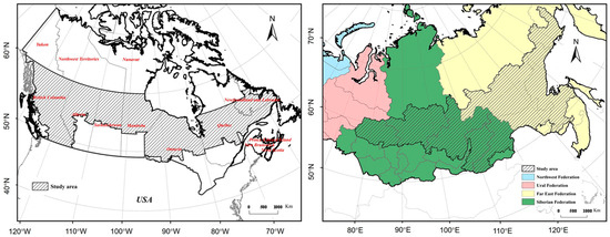
Figure 1.
Geographical location of the study areas ((left), CAN; (right), RUS).
2.1.2. Satellite XCH4 Observations
The comprehensive coverage of atmospheric concentration distribution information is vital for analyzing the spatiotemporal dynamic characteristics of regional atmospheric concentrations. We used the global atmospheric CH4 column concentration (XCH4) monthly data from Lei Liping’s research team from 2010 to 2020 [28]. This dataset was based on geostatistical methods and utilized the intrinsic autocorrelation of satellite observation data (GOSAT and SCIAMACHY satellite data) for optimal estimation, effectively filling the data gap. Based on the spatiotemporal Kriging interpolation method, the generated global XCH4 spatiotemporal continuous grid data were processed with a spatiotemporal resolution of 0.5° grid. The data were in tiff format, which could be used for analyzing the characteristics of global or regional atmospheric CH4 concentration changes. The data collected in this study are presented in Table S1.
2.1.3. Ground-Based XCH4 Data
Based on ground station observation data sourced from the World Data Center for Greenhouse Gases (WDCGG) (https://gaw.kishou.go.jp/ (accessed on 6 July 2023)) and the geographical location of the study area, two atmospheric background stations in Canada were selected (Figure S2). The study area included the East Trout Lake (ETL) and Fraserdale (FSD) stations. The station characteristics are shown in Table S2. Due to the limited number of existing ground stations in Russia, which were not distributed within the RUS study area, this study only used the concentration data from ground stations in the CAN study area as the basis for subsequent validation studies. At the same time, the monthly average CH4 concentration data from the global atmospheric background station in Monaloa, Hawaii (MLO) was selected as a point of comparison. The region is mainly controlled by marine climate and is less affected by local biological activities as well as anthropogenic emissions. The observed values are usually considered representative of the global average water level [29].
2.1.4. Global Biomass-Burning Emission Inventories
Five global biomass burning emission inventories were selected to study the differences and consistency between different inventories (Table S3). (1) GFED4.1s. The Global Fire Emissions Database Version 4.1 covers 14 ecosystem regions around the world from 1997 and presents 0.25° × 0.25° monthly global biomass combustion emissions data. It includes small fire emissions along with satellite information on fire activity and vegetation productivity (https://www.geo.vu.nl/~gwerf/GFED/GFED4/ (accessed on 14 July 2023)). (2) FINN2.5. The Fire Emission Inventory Dataset provides global 0.1° × 0.1° daily fire emission data from 2001 to the present. Currently, the FINN2.5 version dataset provides a distribution map of atmospheric combustion emissions for each component (https://www2.acom.ucar.edu/modeling/finn-fire-inventory-ncar (accessed on 14 July 2023)). (3) GFAS1.2. The Global Fire Assimilation System assimilates fire radiative power (FRP) observations from satellite sensors and provides 0.1° × 0.1° daily near real-time biomass burning emission data of global firepower from 2003 to the present (https://ads.atmosphere.copernicus.eu/cdsapp#!/dataset/cams-global-fire-emissions-gfas?tab=overview (accessed on 14 July 2023)). (4) FEER1.0. The Fire Energy and Emissions Research Dataset measures smoke emission rates using MODIS FRP and aerosol optical depth (AOD) and provides global 0.1° × 0.1° monthly as well as daily real-time biomass burning emission data from 2003 to the present (https://feer.gsfc.nasa.gov/data/ (accessed on 14 July 2023)). (5) QFED2.5. The Rapid Fire Emissions Dataset based on MOD14/MYD14 FRP Level 2 products and emission coefficients is estimated to provide 0.1° × 0.1° monthly and daily biomass burning emission data from 2000 to the present (https://portal.nccs.nasa.gov/datashare/iesa/aerosol/emissions/QFED/ (accessed on 14 July 2023)). According to different estimation methods, there are mainly two GBBEI categories. One is the burned-area-based approach (GFED4.1s, FINN2.5), and the other is the list of products based on the FRP estimation method (FEER1.0, GFAS1.2, QFED2.5) [30].
Since the temporal resolution of GBBEI represents month or day, the spatial resolution is 0.1°~0.25°, while the temporal resolution of the satellite dataset represents month and the spatial resolution is 0.5°~1°. To ensure the consistency between various types of data, the inventory dataset was resampled to 0.25° using the bilinear interpolation method. This method made our data images smooth, without step phenomena, reduced the blackness of linear features, and had higher spatial position accuracy. At the pixel scale, a pixel-by-pixel summation synthesis method was used to generate time series data for the inventory dataset at the monthly and annual scales.
2.2. Methods
2.2.1. Detrended Fluctuation Analysis
Detrended fluctuation analysis (DFA) is a scaling index calculation method proposed by Peng et al. in 1994 based on the DNA mechanism, which was used to analyze the long-range correlation of time series [31]. One advantage of the DFA method is that it can effectively filter out the trend components in the sequence and detect long-range correlations containing noise and superimposed polynomial trend signals. It is suitable for long-range power-law correlation analysis of non-stationary time series. Based on the principle of DFA, we used MATLAB2022 software to subtract an optimal (fitted) line, plane, or surface from the data. The processed data had a mean of zero. The specific formula principle can be found in the Supplementary Materials S1.
2.2.2. Pearson Correlation
The Pearson correlation coefficient (r) is commonly used to measure the linear correlation between variables and global synchronization. Its value ranges from −1 to 1. The closer the absolute value to 1, the stronger the linear correlation between variables. Among them, r > 0 indicates that there is a positive correlation between variables. On the contrary, it indicates there is a negative correlation between variables as well. The specific calculation formula is as follows.
In the equation, {xi, i = 1, 2, …, n} and {yi, i = 1,2, …, n} represent two sets of sequences with a length of n, and and represent the mean values of the two sets of sequences. The t-test is commonly used to test the significance of the Pearson correlation coefficient.
In the formula, n is the number of samples, r is the correlation coefficient, and t is the test value. The commonly used significance test levels are 0.05 (significant correlation) and 0.01 (extremely significant correlation).
2.2.3. Coefficient of Variation
The coefficient of variation (CV) is a statistical analysis method used to measure the magnitude of variability between variables [32]. The coefficient of variation is a standard for converting the degree of variation in variable attributes into a percentage form. It combines the standard deviation and mean of sample variables to describe the degree of variation between sample variables. The specific calculation formula is as follows.
2.2.4. Time Lagged Cross Correlation
Time lag cross-correlation (TLCC) is measured by gradually moving a time series vector and repeatedly calculating the correlation between two signals [33,34]. This method calculates the correlation coefficient of one-time series b with a lag of −k~k order and another time series a. Assuming that the correlation is strongest in order i, it indicates that the optimal lag order is i. If i < 0, then “a” has an i-order with leading The specific calculation formula is as follows.
In the equation, {ai, i = 1,2, …, N} and {bi, i = 1,2, …, N} are two sets of sequences with a length of N. and are the mean values of the two sets of sequences, with k being the order of lag.
2.2.5. Time Series Similarity Measurement—Euclidean Distance
Euclidean distance is the most direct method, and its concept is simple. When applying Euclidean distance to compare two time series, each point between the series establishes a one-to-one correspondence [35]. Based on the correspondence between points, the Euclidean distance is calculated as a distance measure (similarity) between two time series. For the same length sequences, the distance between each two points is calculated and summed. The smaller the distance, the higher the similarity. The specific calculation formula is as follows.
In the equation, {xi, i = 1,2, …, n} and {yi, i = 1,2, …, n} are two sequences of length n.
The studied research method is shown in Figure 2:
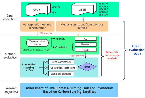
Figure 2.
Flow chart.
3. Results
3.1. Temporal Variation Characteristics of Atmospheric CH4 Concentrations
3.1.1. Monthly Variation Characteristic
Figure 3 shows the time series changes in the atmospheric CH4 concentration in the study area, being monitored by carbon satellites. The global CH4 concentration was observed at selected MLO stations on a monthly scale. Overall, there was a high degree of consistency in the time trends between the two data sources in different research areas. The concentration of XCH4 in the atmosphere showed a significant fluctuating upward trend between 2010 and 2020. Considering the specific values (Figure 3), the change trend for CAN was consistent with the global atmospheric CH4 concentration change trend. The atmospheric CH4 concentrations in the CAN (average value: 1804.45 ± 25.60 ppb) and RUS (average value: 1811.44 ± 26.38 ppb) areas were lower than the global average (average value: 1834.26 ± 26.51 ppb). Notably, the time series change trend for CAN lagged behind the global atmospheric CH4 concentration change trend, whereas that for RUS was the opposite. We assumed that this was related to the timing of large-scale forest fires in the study areas, which would bring inconsistent peak changes.
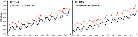
Figure 3.
Monthly average changes in satellite data for XCH4 (ppb) in areas affected by forest fires and globally (black—satellite data, red—MLO station, blue—linear fitting line for satellite data). The global monthly XCH4 trend is expressed as: y = 0.6807x + 1789, R2 = 0.9575.
Although large-scale synchronous monitoring can be accomplished using the atmospheric methane column concentration, retrieved from satellite remote sensing observation data [29], there are some limitations to the accuracy of satellite remote sensing observations compared to ground station observations. Therefore, monthly data from ETL and FSD stations within the CAN region were collected in this study, using the average level as the ground observation value. Since the data product retrieved by satellite is the average mole fraction of dry air in the CH4 column after full mixing of the atmosphere (Figure 4a), it is more diluted than the surface data. Therefore, the observation value at ground stations was higher than the satellite remote sensing retrieval data. Although there were differences in specific values between the two datasets, their time series trends were relatively similar. The difference (130.08 ± 10.16 ppb) between 2010 and 2020 showed good stability without significant seasonal fluctuations. This could explain the phenomenon of differences between satellites and MLO sites in Figure 1. Due to the global average presented by MLO sites, it was difficult to accurately reflect the gas concentration in a specific region.
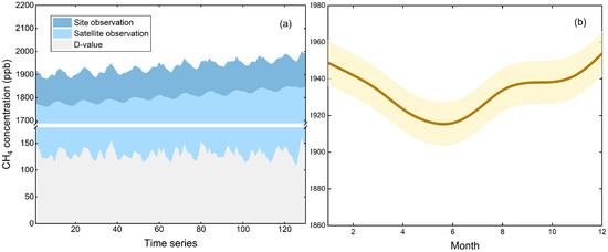
Figure 4.
(a) Actual values of satellite monitoring and ground station observations from 2010 to 2020 (D-value: difference between site observation and satellite observation); (b) multi-year monthly average CH4 concentrations and standard deviations (solid lines represent multi-year monthly average concentrations, and filling on both sides represents standard deviations).
3.1.2. Seasonal Variation Characteristic
The relative change on a monthly scale cannot be reflected only from the absolute change trend analysis of atmospheric concentration. By removing linear trends from the data through detrended fluctuation analysis [35], we focused on the fluctuation of trend data. In order to obtain the relative variation of the data, the annual relative variation values from the concentration data were extracted after removing the trend. The temporal variation differences for XCH4 in the CAN and RUS regions from 2010 to 2020 were obtained (ΔXCH4 referred to the difference between the annual mean of atmospheric CH4 concentration in the following year and the previous year) (Figure 5). The pretreated atmospheric methane column concentrations can be used as indicators to evaluate the methane source/sink of the study area relative to the regional average level [21]. As shown in Figure 5, there was a significant difference in the trend of atmospheric CH4 concentration changes between the two regions. The peak value in the CAN region was in October, and the valley value was in March. The values from August to December were positive. This indicated that the region was a methane source during these months. The atmospheric methane concentration showed a positive growth trend. However, the peak value in the RUS region was in August, and the valley value was in March. The values from July to September were greater than zero. Other months showed a decreasing trend. Due to lower temperatures in the RUS region compared to the CAN region, methane concentration changes showed a negative increase in winter.
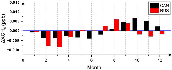
Figure 5.
Seasonal variation in atmospheric concentrations from 2010 to 2020.
At the same time, the seasonal variation in CH4 concentrations at atmospheric background stations in the CAN region was analyzed in this study. Moreover, the multi-year monthly average and standard deviation of atmospheric CH4 concentration were obtained while considering the average of two stations (Figure 4b). It showed atmospheric methane concentrations were low from April to July. Among them, the highest value of atmospheric CH4 concentration was in December (1953.74 ± 12.04 ppb), and the lowest value of atmospheric CH4 concentration was in June (1914.20 ± 12.04 ppb). Due to the unstable chemical properties of methane, illumination factors could lead to the oxidation of methane in the atmosphere [29] while resulting in a low value in summer.
3.1.3. Interannual Variation Characteristic
Considering annual changes (Figure 6a), there is a significant interannual fluctuation in atmospheric CH4 concentrations in various regions, with alternating positive and negative annual changes. However, the years of increase in both are not the same. In the CAN region, the atmospheric CH4 concentration showed positive growth in 2014, 2016, 2017, 2019 and 2020, with significant increases in 2014 and 2020. In the RUS region, the atmospheric CH4 concentration showed positive increases in 2014, 2016, 2018 and 2020, with significant increases in 2016 and 2020. The sudden increment represents the occurrence of abnormal activities that could have generated a large amount of CH4 during that year. As the study area included a typical region of global forest fires, it was found that the year with a sudden increment was closely related to historical events after considering historical forest fire events in the region. According to the interannual variation analysis of CH4 concentration observed by atmospheric background stations in the CAN region, the trend of atmospheric CH4 variation observed by ground stations was consistent and demonstrated a continuous upward trend (Figure 6b). During the observation period, the annual average growth rate of the atmospheric CH4 concentration was 0.37%, indicating a strong growth trend.
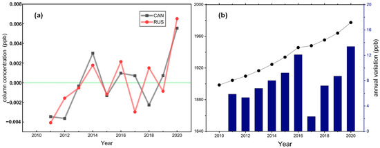
Figure 6.
(a) Year-to-year Δ XCH4 changes for the period 2010–2020. (b) The interannual variation in CH4 concentration at atmospheric background stations in the CAN region.
3.2. Temporal Variation Characteristics of CH4 Emissions
3.2.1. Monthly Variation Characteristic
The average CH4 emissions from the five emission inventory datasets showed significant fluctuations over time, with emissions rising from April to October each year (Figure 7). The overall emissions in RUS were higher than those in the CAN research area. This could be attributed to the fact that the forest area in Russia is the largest in the world, and forest fires are frequent. As shown in Figure 7, the estimated total emissions for the five emission inventories in the CAN study area from 2010 to 2020 ranged from 2.02 to 5.84 Tg CH4, while estimates for the RUS study area ranged from 3.97 to 14.23 Tg CH4. Among them, the estimated methane emissions from the GFED4s were the highest, while the QFED2.5 was relatively conservative. Based on the comprehensive (five types) emission inventory datasets, there were consistent mutation months in the CAN and RUS regions in 2018 and 2012 and 2019, respectively. The RUS region had few forest fires and no greenhouse gas emissions in winter due to the cold and dry climate.
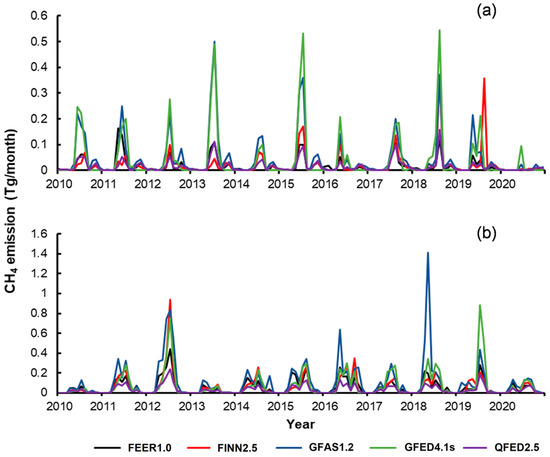
Figure 7.
Monthly time series changes in CH4 emissions from different inventory datasets: (a) CAN; (b) RUS.
3.2.2. Seasonal Variation Characteristic
As shown in Figure 8, there was a significant seasonal difference in CH4 emissions between the CAN and RUS regions, both exhibiting a seasonal cycle of highs in summer and autumn and lows in winter and spring. In other words, emissions showed a continuously increasing peak from May to September, indicating that forest fires are more common in the two regions during this period. Moreover, the box plot (Figure S3) shows that emission data were relatively scattered, reflecting the instantaneous and uncertain characteristics of gas emissions. Among them, the highest CH4 emissions occurred in July (CAN average: 0.11 Tg CH4, RUS average: 0.22 Tg CH4), and the lowest in January. This could be attributed to large-scale forest fires [36], mainly due to high summer temperatures and dry environment while resulting in an increase in the emissions of CH4 and other gases. However, the two study areas had extremely low air temperatures and ice formation in January, making them less prone to fires.
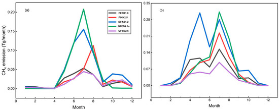
Figure 8.
Seasonal changes in CH4 emissions from 2010 to 2020: (a) CAN; (b) RUS.
3.2.3. Interannual Variation Characteristic
Except for the inconsistent years of FEER data mutation, most datasets showed consistent interannual trends in CH4 emissions (Figure 9). The estimated emissions for all datasets decreased slightly in the CAN region between 2010 and 2020 while slightly increasing in the RUS region. However, the interannual variation trend in CH4 emissions in the CAN and RUS research areas was not significant. The highest CH4 emissions in the CAN region were in 2013. There were small peaks in 2015 and 2018. This result can be explained by the phenomenon of El Niño drought years (2013 and 2015). The highest CH4 emissions in the RUS region occurred in 2012, with small peaks in 2016 and 2018. Based on the variation analysis numerical coefficient (Table S4), the estimated CH4 emissions from different datasets in the CAN region generally exhibited a high fluctuation trend (41.03% < CV < 60.70%), with an average CH4 emission value of 0.31 ± 0.17 Tg CH4 (±1 Std) and an average value of 0.18 ± 0.07~0.52 ± 0.29 Tg CH4 for each dataset. Similarly, the CH4 emissions in the RUS region also exhibited a high fluctuation trend (43.77% < CV < 62.01%), with the average values of each dataset ranging from 0.36 ± 0.16 to 1.27 ± 0.79 Tg CH4. Among them, the differences in the average emissions of each inventory were within a certain range. Figure 10 and Figure 11 show the similarities and differences in the spatial distribution of annual methane emissions. Five inventories showed consistent spatial heterogeneity in terms of annual total methane emissions, exhibiting a characteristic of spatial aggregation while also exhibiting differences in spatial numerical distribution. Except in the CAN region, the spatial distribution of methane emissions from GFED4.1s was different from those of the other four inventories, with fewer emissions in the southwest. In the CAN area, it was mainly concentrated in British Columbia and Alberta, and in the RUS area, it was concentrated in Amur Oblast.
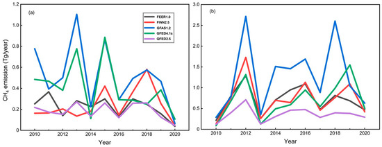
Figure 9.
Annual changes in CH4 emissions from 2010 to 2020: (a) CAN; (b) RUS.

Figure 10.
Spatial distribution of annual total methane emissions in the CAN region.
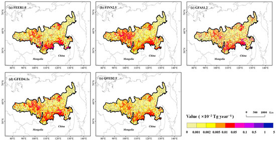
Figure 11.
Spatial distribution of annual total methane emissions in the RUS region.
3.3. Analysis of the Temporal Correlation between Atmospheric CH4 Concentration and CH4 Emissions
3.3.1. Ground Station Data and Satellite Data
Domestic and international research frequently uses ground station observation data and satellite remote sensing inversion data to verify the reliability of both. In order to verify the accuracy of remote sensing data, fitting regression analysis was first conducted on ground station data and satellite data in the CAN region from 2010 to 2020. By establishing a linear regression model, the correlation between the two datasets was obtained (Figure S4). The results indicated that the satellite inversion of CH4 concentration data (XCH4) used by the research institute had good consistency with ground observations of CH4 concentrations in time series (R2 = 0.93). It was evident that there was a high temporal correlation between satellite data and ground observation station data, and at the same time, ground stations could not fully cover the research area. Therefore, the CH4 concentrations retrieved from satellite remote sensing could be used as a measurement standard to evaluate the authenticity and accuracy of estimated values in various inventory datasets.
3.3.2. Analysis of Correlations between Inventory Datasets and between Inventory Datasets and Satellite Datasets
Based on preliminary data experiments, it was found that the changes in CH4 emissions at the interannual scale did not reflect the real-time characteristics of emissions. The interannual differences between inventory data and satellite data were significant due to the accumulation of annual values. Therefore, the correlation between inventory data and satellite data at the monthly scale (multi-year monthly average) was considered for analysis. As shown in Figure S5, there was a significant positive correlation between the estimated emissions from the five inventory datasets on monthly scales. However, the estimated emissions from the inventory datasets showed a negative correlation with the changes in atmospheric CH4 concentrations monitored by satellites. Therefore, it was assumed that a lagging effect was present in between.
In order to further understand the lag time between emissions and changes in atmospheric concentrations, the optimal lag order between gas emissions and changes in atmospheric concentrations was considered. Figure 12 shows the gradient distribution diagram of the Pearson correlation coefficient between the atmospheric concentration change and gas emissions in the CAN and RUS regions using the TLCC. As shown in Figure 12a, when the atmospheric CH4 concentration change lagged behind the CH4 emissions for 3 months, the correlation between the two was the strongest in the CAN region. Except for FINN2.5, the correlation coefficient under the optimal lag order was above 0.9 for all other datasets, and the significance was p < 0.01 (Figure S6a). In the RUS region, the optimal lag order for atmospheric CH4 concentration change was 1. Except for GFAS1.2, the correlation coefficients of all other datasets were above 0.8 and indicated a significant correlation when the lag time was 1 month (Figure S6b).
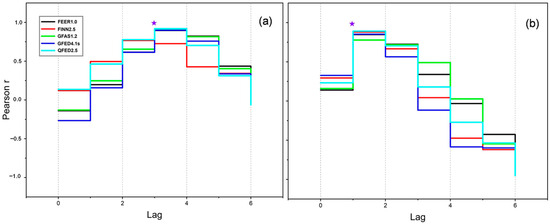
Figure 12.
Time lag cross-correlation analysis of emissions and atmospheric concentration changes (purple star—optimal lagging order): (a) CAN; (b) RUS.
The lagging effect of inventory emissions and atmospheric concentration changes in the CAN and RUS regions were eliminated based on the optimal lag order. As shown in Figure 13, the satellite Δ XCH4 exhibited a non-linear temporal variation, which was consistent with the inventory CH4 emissions. In this study, the change in atmospheric methane concentrations monitored by satellites was used as the standard to judge the quality of each inventory dataset. The Euclidean distance in the time series similarity measurement method was used to compare the satellite-measured concentrations after eliminating the lagging effects and five emission inventories [35]. As shown in Figure 14, the “distance” between the estimated CH4 emissions from the QFED2.5 inventory and the time series of satellite data to eliminate lagging effects was the smallest for both the CAN and RUS regions, indicating the highest similarity between the two. Based on consistency analysis of satellite data, the QFED2.5 emission inventory dataset performed better than other emission inventories (discussed in Section 4.1). It was consistent with the simulation results of Su et al. (2023) [17].
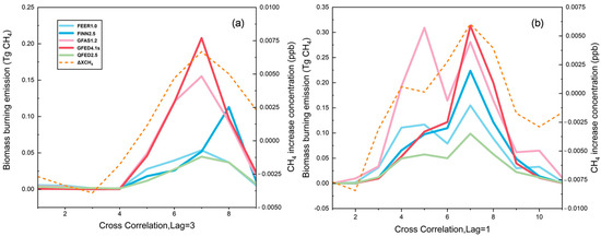
Figure 13.
Time variation trend between CH4 emissions inventories and satellite concentrations for eliminating lagging effects: (a) CAN; (b) RUS.
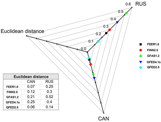
Figure 14.
Euclidean distance between emissions inventories and satellite concentrations for eliminating lagging effects.
4. Discussion
The temporal similarities and differences between the five existing GBBEI datasets and satellite monitoring datasets were discussed in this study. As demonstrated in this study, the QFED2.5 dataset had temporal trend more similar to that for satellite concentration data compared to the other inventories. Detailed explanations for the differences between the five GBBEIs will be discussed in Section 4.1, and explanations for lagging effect will be discussed in Section 4.2. The uncertainty in selecting the study area is discussed in Section 4.3.
4.1. Possible Explanations for Differences among the GBBEIs
This study showed that the estimated methane emissions from the QFED2.5 emission dataset in the CAN and RUS regions were consistently lower than those based on other datasets, while estimates based on GFED4.1s were consistently higher than those based on other datasets. Some possible reasons for these differences could be as follows.
The results for inventories based on FRP (QFED2.5) were lower than those based on burned area estimation (GFED4.1s) mainly due to the use of different remote sensing datasets and the physical differences between the forests. Therefore, the FRP generated by active fire detection was underestimated, while the fire area detected over the burned area was overestimated [36]. The reasons for this phenomenon are as follows: The locations, sizes and numbers of individual fires within the active fire pixels were unknown, and the active fire pixel may have been smaller than the occupied area of the actual fire perimeter. This was particularly significant in the northern forest areas [37]. Due to the spatial resolution of satellite data, the burned area is often overestimated. As the spatial resolution of MODIS burned area products is 500 m, when a small fire occurs (less than 500 m × 500 m), the entire pixel is assigned as burned out. This indicates that pixels are often misclassified as completely burned-out pixels [38]. Moreover, when using FRP derived from MODIS sensors, the average radiation power of northern forest fires is significantly lower compared to other regions (ex: North America), and this difference is related to the physical differences between forests. MODIS could not detect low-intensity fires in high-latitude areas and was also hindered by cloud cover [39]. Based on the above analysis, our results showed a high GFED4.1s and a low QFED2.5, mainly due to overestimation of the over fire area of the burned area products, as well as limitations in extracting fire radiative power from FRP derived from MODIS active fire products in high-latitude areas of northern forests.
There may be discrepancies in the input parameters when estimating the five types of inventories. The burned-area-based approach supports the monitoring of areas and can effectively evaluate the combustion emissions of large fires [40]. For example, compared to other inventories, GFED4.1s uses the MCD64A1 product, covering small fires that may be missed and resulting in higher estimated methane emissions. Although FINN1.5 is also a burned-area-based product, its combustion area estimation is relatively simple without complex spatial and temporal variability. It estimates the burned area of each fire pixel for all biomass types under one square kilometer. Compared to the estimation method based on area, the FRP-based approach has better monitoring effectiveness for small fires and short-term agricultural fires [41]. For FEER1.0, the process of deriving Ce (coefficient of smoke emission) is limited by MODIS AOD, which limits the impact of other emission sources [42]. Although GFAS1.0 uses the FRP method to estimate emissions, its emission coefficient is obtained through linear regression with the GFED3.1 dry matter combustion rate. Therefore, its emissions calculation is similar to that of the GFED series. Compared to other datasets, QFED2.5 combines the cloud correction method developed in GFAS1.0 and adopts more complex non-observational (ex: cloud obscuration) land area processing methods [43]. Therefore, this operation can filter out misjudged fire point pixels to a higher extent. In addition, the estimation method based on FRP can directly estimate the fuel consumption of energy released from fires, without being affected by uncertainties related to estimated fuel load and combustion integrity. Its combustion conversion rate is not affected by surface vegetation types [44] and could prevent the accumulation of multiple factor errors and reduce the uncertainty of emission estimation [45,46]. Although there were differences in the values between inventories in this study, they showed good consistency in their temporal trends. At the same time, it is currently difficult for the datasets to evaluate accurate emission values. Most studies compared the superiority of the inventory dataset to the trend consistency between the datasets [47,48]. Therefore, the level of the values cannot be used as a standard to measure the accuracy of inventory estimation. Moreover, in Section 3.3.2, we found that the coefficient of correlation for QFED2.5 with each inventory was above 0.8 (Figure S5), and its “similarity distance” with satellite data was the shortest (below 0.14). Based on the above possible reasons and the similar results with QFED2.5 as well as satellite concentration data obtained in this study, QFED2.5 was found to be superior to other biomass-burning emission inventories.
4.2. Explanation of the Lagging Effect
Considering the above analysis results, lagging effects were found to be present between the atmospheric methane concentration monitored by satellite and methane emissions estimated in the inventory. In this section, this phenomenon is verified, and a trend analysis is conducted on the atmospheric methane concentration as well as methane emissions before and after the severe forest fire events in the CAN and RUS regions from 2010 to 2020.
According to Figure 9b, the methane emissions from GBBEI in the RUS region were highest in 2012. The number of hotspots in the region from 2011 to 2013 was obtained (Figure 15) based on the FIRMS Active Fires on Earth Engine APP (https://globalfires.earthengine.app/view/firms (accessed on 14 July 2023)). As shown in Figure 15, 699,218 hotspots were detected in 2012, with the highest number of hot spots being 240,746 in July 2012, followed by May and June. The number of hotspots detected in these three months accounted for 72.02% of all hotspots detected in 2012. According to the Global Disaster Data Platform statistics (https://www.gddat.cn/newGlobalWeb/#/DisasBrowse (accessed on 6 July 2023)), a severe forest fire occurred in Siberia, Russia, in the summer of 2012. Based on the obtained fire points, a consistent analysis was conducted on the methane emissions and satellite concentrations before and after the wildfires in the RUS region in 2012. Similarly, based on Figure 9b and historical fire events, the year (2015) with consistent peak values for each inventory was designated as the year of severe fire occurrence in the CAN region. As shown in Figure 16, the atmospheric methane concentrations monitored by satellite lagged the methane emissions estimated by the inventories by about 2–3 months in the CAN area in 2015, whereas the serious forest fire event in the RUS area in 2012 lagged by about 0–1 month. This result is consistent with the multi-year monthly average data in Section 3.3.2. Therefore, two main reasons for the lagging effect can be proposed. First, there could be a corresponding time difference in the concentration changes received by carbon-monitoring satellites due to the distance required for the transmission of gas emissions to carbon satellite sensors. Second, the length of the lag time could be related to the amount of gas emissions. As shown in Figure 16, the methane emissions in the RUS region were about twice those of the CAN region. The larger the gas emissions in the region, the more severe the forest fire. This could be attributed to the greater heat released by the fire, the higher the rate of gas production [49] and the shorter the time to reach the carbon satellite sensor.
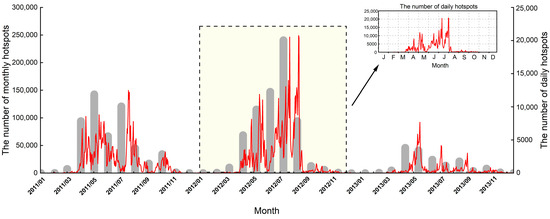
Figure 15.
The number of daily (red line) and monthly (grey column) hotspots in the RUS region from 2011 to 2013.
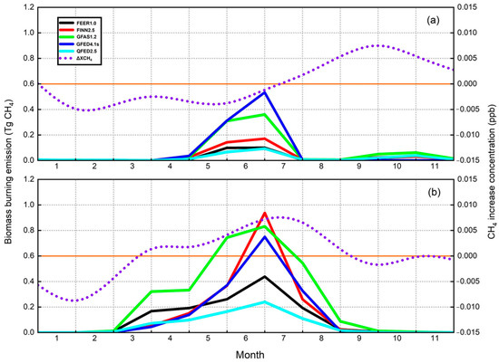
Figure 16.
Time variation trends of atmospheric methane concentrations monitored by satellite and methane emissions estimated by inventories during the most serious fire events from 2010 to 2020: (a) CAN: 2015; (b) RUS: 2012.
4.3. Uncertainty in the Selection of Research Areas
Due to the uncertainty in selecting reference data for the study area such as the MCD64A1 burned area map, MCD12Q1 land cover type map and the global forest loss driver classification map, our results were affected to some extent. MCD64A1 burned area data usually have a certain degree of overestimation because of their spatial resolution (500 m). When a small fire occurs (less than 500 m × 500 m), the entire pixel needs to be assigned as burned, which affected the selection of our research area [38]. The classification accuracy of MCD12Q1 land cover type data is lower than official standards [50]. At the same time, we chose the land cover from 2015 to represent the period from 2010 to 2020, which may have presented some shortcomings. The classification map of global forest loss drivers showed that in northern forests, especially in Russia, wildfires spread to previously logged areas or occurred after the fire. In these cases, it was difficult to attribute a single driving factor to these regions, as there were patterns of multiple driving factors within the same unit, despite being in different years during the analysis period (2001–2015). Moreover, the time range involved in this map had a certain impact on our research results [25]. We used the method of geographic weighted overlay analysis to determine our research areas. According to the setting of weight coefficients, the MCD64A1 burned area map contributed 15%, the MCD12Q1 land cover type map contributed 35%, and the global forest loss driver classification map contributed 50% to the uncertainty of the results.
5. Conclusions
Five commonly used GBBEIs, atmospheric concentration satellite data and ground station observation concentration data were selected in this study. Considering the typical area of global forest fires—the boreal forest as an example—CH4 with a lifespan of 10 years was used as the research object, and methods such as numerical comparison, trend consistency analysis and time lag cross-correlation analysis were adopted. The consistency and differences in time scales between different datasets from 2010 to 2020 were shown at the regional scale. The connection between emissions and atmospheric concentrations was thoroughly investigated. Using atmospheric concentrations observed by satellites as the standard, the datasets among existing GBBEIs were evaluated. In this study, we found a lagging effect to be present between the methane emissions estimated from the inventory datasets and the atmospheric methane concentrations observed by satellites. The lag time was not consistent in different regions. Furthermore, based on the measurement of time series similarity and previous research results, the QFED2.5 was found to be a more reliable inventory.
The relationship between CH4 emissions and atmospheric concentration changes in forest fire areas was investigated. By using the method of “atmospheric concentration measurement assisting inventory validation”, the reliability of existing GBBEIs was qualitatively evaluated, providing a reference for selecting appropriate GBBEIs in “bottom-up” inventory estimation research. Given the uncertainty and shortcomings of the existing inventory estimation, our analysis work could be helpful in the future by applying a higher spatiotemporal resolution and smaller unit fire events.
Supplementary Materials
The following supporting information can be downloaded at: https://www.mdpi.com/article/10.3390/rs15184547/s1, S1: Detrended fluctuation analysis calculation steps and formulas; Figure S1: Global forest disturbance drivers map; Figure S2: Distribution map of CAN regional stations; Figure S3: Seasonal box chart of CH4 emissions from 2010 to 2020 (black hollow circle: mean value, red solid line: median value, black diamond: outlier): (a) CAN; (b) RUS; Figure S4: Ground station data and observed remote sensing atmospheric concentration data; Figure S5: Correlation analysis between inventory dataset and atmospheric CH4 concentration data from 2010 to 2020: (a) CAN; (b) RUS; Figure S6: Correlation number between atmospheric concentration change and gas emission under optimal lag number (red star represents p < 0.01): (a) CAN; (b) RUS; Table S1: Data collection details; Table S2: Characteristics of two atmospheric background stations and MLO stations in the CAN region; Table S3: Summary of five biomass burning emission inventories; Table S4: Average CH4 emissions and standard deviation in CAN and RUS regions from 2010 to 2020.
Author Contributions
Conceptualization, S.Z. and L.W.; methodology, S.Z.; software, S.Z.; validation, S.Z.; formal analysis, S.Z., Y.S. and Z.Z.; investigation, S.Z.; resources, S.Z.; data curation, S.Z.; writing—original draft preparation, S.Z.; writing—review and editing, S.Z., L.W., Y.S., Z.Z., B.N. and Z.N.; visualization, S.Z., Y.S. and Z.Z.; supervision, L.W.; project administration, L.W.; funding acquisition, L.W. All authors have read and agreed to the published version of the manuscript.
Funding
This work was supported by the National Key Research and Development Program of China (2021YFE0117900); the National Natural Science Foundation of China [grant numbers U2244230].
Data Availability Statement
The data presented in this study are available on request from the corresponding author. The data are not publicly available due to privacy reasons.
Acknowledgments
We are grateful for the atmospheric CH4 column concentration product dataset provided by Lei. L’s team from the website at (https://data.casearth.cn/sdo/detail/6253cddc819aec49731a4bc4 (accessed on 14 July 2023)). We thank the World Data Centre for Greenhouse Gases (WDCGG) for providing XCH4 observed data products at (https://gaw.kishou.go.jp/ (accessed on 14 July 2023)).
Conflicts of Interest
The authors declare no conflict of interest.
References
- Kim, Y.; Tanaka, N.; Fukuda, M.; Kushida, K. Effect of forest fire on fluxes of CH4 and N2O in boreal forest soils, interior Alaska. In Non-CO2 Greenhouse Gases: Scientific Understanding, Control Options and Policy Aspects. Proceedings of the Third International Symposium, Maastricht, The Netherlands, 21–23 January 2002; Millpress Science Publishers: Rotterdam, The Netherlands; pp. 55–60.
- Koster, E.; Koster, K.; Berninger, F.; Aaltonen, H.; Zhou, X.; Pumpanen, J. Carbon dioxide, methane and nitrous oxide fluxes from a fire chronosequence in subarctic boreal forests of Canada. Sci. Total Environ. 2017, 601, 895–905. [Google Scholar] [CrossRef] [PubMed]
- Fu, X. The impact of forest fire on forest ecosystem. Mod. Agric. Res. 2021, 27, 101–103. [Google Scholar] [CrossRef]
- Chao, D. The Impact of Phenological Changes in Northern Forests on Carbon Budget. Master’s Thesis, Northeast Normal University, Changchun, China, 2020. [Google Scholar]
- Wooster, M.J.; Zhang, Y.H. Boreal forest fires burn less intensely in Russia than in North America. Geophys. Res. Lett. 2004, 31. [Google Scholar] [CrossRef]
- Stocks, B.J.; Fosberg, M.A.; Lynham, T.J.; Mearns, L.; Wotton, B.M.; Yang, Q.; Jin, J.Z.; Lawrence, K.; Hartley, G.R.; Mason, J.A.; et al. Climate change and forest fire potential in Russian and Canadian boreal forests. Clim. Chang. 1998, 38, 1–13. [Google Scholar] [CrossRef]
- Bai, Y.; Wang, B.; Wu, Y.; Liu, X. Experimental study on pyrolysis of surface litter of main forest types in Changbai Mountains. Fire Sci. Technol. 2022, 41, 705–709. [Google Scholar] [CrossRef]
- Wu, Y.; Shu, F.; Wang, M.; Zhang, H.; Si, L. A review of forest fires worldwide in recent years. J. Temp. For. Res. 2022, 5, 49–54. [Google Scholar] [CrossRef]
- Levine, J.S.; Cofer, W.R., III; Cahoon Jr, D.R.; Winstead, E.L. A driver for global change. Environ. Sci. Technol. 1995, 29, 120A–125A. [Google Scholar] [CrossRef]
- Feng, L.; Palmer, P.I.; Zhu, S.H.; Parker, R.J.; Liu, Y. Tropical methane emissions explain large fraction of recent changes in global atmospheric methane growth rate. Nat. Commun. 2022, 13, 1378. [Google Scholar] [CrossRef]
- Song, H.; Sheng, M.; Lei, L.; Guo, K.; Zhang, S.; Ji, Z. Spatial and Temporal Variations of Atmospheric CH4 in Monsoon Asia Detected by Satellite Observations of GOSAT and TROPOMI. Remote Sens. 2023, 15, 3389. [Google Scholar] [CrossRef]
- Guo, M.; Li, J.; Xu, J.; Wang, X.; He, H.; Wu, L. CO2 emissions from the 2010 Russian wildfires using GOSAT data. Environ. Pollut. 2017, 226, 60–68. [Google Scholar] [CrossRef]
- Goto, Y.; Suzuki, S. Estimates of carbon emissions from forest fires in Japan, 1979–2008. Int. J. Wildland Fire 2013, 22, 721–729. [Google Scholar] [CrossRef]
- Guo, L.F.; Ma, Y.F.; Tigabu, M.; Guo, X.B.; Zheng, W.X.; Guo, F.T. Emission of atmospheric pollutants during forest fire in boreal region of China. Environ. Pollut. 2020, 264, 114709. [Google Scholar] [CrossRef]
- Zhao, Y. Research on High-Resolution Multi-Year Emission Inventory of Biomass Combustion in Northeast China from 2001 to 2017. Master’s Thesis, Harbin Normal University, Harbin, China, 2020. [Google Scholar]
- Shi, Y.S.; Matsunaga, T. Temporal comparison of global inventories of CO2 emissions from biomass burning during 2002–2011 derived from remotely sensed data. Environ. Sci. Pollut. Res. 2017, 24, 16905–16916. [Google Scholar] [CrossRef] [PubMed]
- Su, M.Q.; Shi, Y.S.; Yang, Y.L.; Guo, W.Y. Impacts of different biomass burning emission inventories: Simulations of atmospheric CO2 concentrations based on GEOS-Chem. Sci. Total Environ. 2023, 876, 162825. [Google Scholar] [CrossRef] [PubMed]
- Xu, Y. Study on Evolution Characteristics and Dynamic Estimations of Open Biomass Burning Emissions, in China. Ph.D. Thesis, South China University of Technology, Guangzhou, China, 2020. [Google Scholar]
- Harrison, S.P.; Bartlein, P.J.; Brovkin, V.; Houweling, S.; Kloster, S.; Prentice, I.C. The biomass burning contribution to climate-carbon-cycle feedback. Earth Syst. Dyn. 2018, 9, 663–677. [Google Scholar] [CrossRef]
- Janardanan, R.; Maksyutov, S.; Ito, A.; Yukio, Y.; Matsunaga, T. Assessment of Anthropogenic Methane Emissions over Large Regions Based on GOSAT Observations and High Resolution Transport Modeling. Remote Sens. 2017, 9, 941. [Google Scholar] [CrossRef]
- Shi, Y.S.; Matsunaga, T.; Noda, H. Interpreting Temporal Changes of Atmospheric CO2 Over Fire Affected Regions Based on GOSAT Observations. IEEE Geosci. Remote Sens. Lett. 2017, 14, 77–81. [Google Scholar] [CrossRef]
- Chevallier, F.; Broquet, G.; Zheng, B.; Ciais, P.; Eldering, A. Large CO2 Emitters as Seen from Satellite: Comparison to a Gridded Global Emission Inventory. Geophys. Res. Lett. 2022, 49, e2021GL097540. [Google Scholar] [CrossRef]
- Köster, E.; Köster, K.; Berninger, F.; Pumpanen, J. Carbon dioxide, methane and nitrous oxide fluxes from podzols of a fire chronosequence in the boreal forests in Värriö, Finnish Lapland. Geoderma Reg. 2015, 5, 181–187. [Google Scholar] [CrossRef]
- Köster, E.; Köster, K.; Berninger, F.; Prokushkin, A.; Aaltonen, H.; Zhou, X.; Pumpanen, J. Changes in fluxes of carbon dioxide and methane caused by fire in Siberian boreal forest with continuous permafrost. J. Environ. Manag. 2018, 228, 405–415. [Google Scholar] [CrossRef]
- Curtis, P.G.; Slay, C.M.; Harris, N.L.; Tyukavina, A.; Hansen, M.C. Classifying drivers of global forest loss. Science 2018, 361, 1108–1111. [Google Scholar] [CrossRef] [PubMed]
- Romanov, A.A.; Tamarovskaya, A.N.; Gloor, E.; Brienen, R.; Gusev, B.A.; Leonenko, E.V.; Vasiliev, A.S.; Krikunov, E.E. Reassessment of carbon emissions from fires and a new estimate of net carbon uptake in Russian forests in 2001–2021. Sci. Total Environ. 2022, 846, 157322. [Google Scholar] [CrossRef] [PubMed]
- Ding, Q.; Feng, X. Change Analysis of Boreal Forest Fire Using MODIS Thermal Anomalies Product for European Russia. J. Geo-Inf. Sci. 2013, 15, 476–482. [Google Scholar] [CrossRef]
- Lei, L.; Song, H.; Li, L.; Zeng, Z.; He, Z. Global 50 km GOSAT and SCIAMACHY Atmospheric CH4 Column Concentration Product Data Set from 2003 to 2021; Aerospace Information Innovation Institute of the Chinese Academy of Sciences: Beijing, China, 2021. [Google Scholar] [CrossRef]
- Zhang, S. A Study of Atmospheric CH4 Concentration Spatio-Temporal Variation and Its Response to Anthropogenic Emissions in China Based on the Ground-Based and Satellite Observations. Master’s Thesis, East China Normal University, Shanghai, China, 2022. [Google Scholar]
- Pan, X.H.; Ichoku, C.; Chin, M.; Bian, H.S.; Darmenov, A.; Colarco, P.; Ellison, L.; Kucsera, T.; da Silva, A.; Wang, J.; et al. Six global biomass burning emission datasets: Intercomparison and application in one global aerosol model. Atmos. Chem. Phys. 2020, 20, 969–994. [Google Scholar] [CrossRef]
- Xu, Z.; Wan, J.W.; Li, G.; Su, F. Target Detection within Sea Clutter Based on Multifractal Detrended Fluctuation Analysis. Adv. Eng. Forum 2012, 4, 259–262. [Google Scholar] [CrossRef]
- Kvalseth, T.O. Coefficient of variation: The second-order alternative. J. Appl. Stat. 2017, 44, 402–415. [Google Scholar] [CrossRef]
- Podobnik, B.; Stanley, H.E. Detrended cross-correlation analysis: A new method for analyzing two nonstationary time series. Phys. Rev. Lett. 2008, 100, 084102. [Google Scholar] [CrossRef]
- Shen, C.H. Analysis of detrended time-lagged cross-correlation between two nonstationary time series. Phys. Lett. A 2015, 379, 680–687. [Google Scholar] [CrossRef]
- Agrawal, R.; Faloutsos, C.; Swami, A. Efficient similarity search in sequence databases. In Foundations of Data Organization and Algorithms, Proceedings of the 4th International Conference, FODO’93, Chicago, IL, USA, 13–15 October 1993; Springer: Berlin/Heidelberg, Germany, 1993; pp. 69–84. [Google Scholar]
- Van der Werf, G.R.; Randerson, J.T.; Giglio, L.; Collatz, G.J.; Kasibhatla, P.S.; Arellano, A.F. Interannual variability in global biomass burning emissions from 1997 to 2004. Atmos. Chem. Phys. 2006, 6, 3423–3441. [Google Scholar] [CrossRef]
- van Wees, D.; van Der Werf, G.R.; Randerson, J.T.; Andela, N.; Chen, Y.; Morton, D.C. The role of fire in global forest loss dynamics. Glob. Chang. Biol. 2021, 27, 2377–2391. [Google Scholar] [CrossRef]
- Shi, Y.S.; Sasai, T.; Yamaguchi, Y. Spatio-temporal evaluation of carbon emissions from biomass burning in Southeast Asia during the period 2001–2010. Ecol. Model. 2014, 272, 98–115. [Google Scholar] [CrossRef]
- Roberts, G.; Wooster, M.J.; Freeborn, P.H.; Xu, W. Integration of geostationary FRP and polar-orbiter burned area datasets for an enhanced biomass burning inventory. Remote Sens. Environ. 2011, 115, 2047–2061. [Google Scholar] [CrossRef]
- Randerson, J.T.; Chen, Y.; van der Werf, G.R.; Rogers, B.M.; Morton, D.C. Global burned area and biomass burning emissions from small fires. J. Geophys. Res.-Biogeosci. 2012, 117. [Google Scholar] [CrossRef]
- Giglio, L.; Randerson, J.T.; Van Der Werf, G.R. Analysis of daily, monthly, and annual burned area using the fourth-generation global fire emissions database (GFED4). J. Geophys. Res. Biogeosci. 2013, 118, 317–328. [Google Scholar] [CrossRef]
- Ichoku, C.; Ellison, L. Global top-down smoke-aerosol emissions estimation using satellite fire radiative power measurements. Atmos. Chem. Phys. 2014, 14, 6643–6667. [Google Scholar] [CrossRef]
- Darmenov, A.; da Silva, A. The Quick Fire Emissions Dataset (QFED): Documentation of Versions 2.1, 2.2 and 2.4. In Technical Report Series on Global Modeling and Data Assimilation; NASA TM-2013-104606; NASA: Washington, DC, USA, 2015; Volume 32, p. 183. [Google Scholar]
- Wooster, M.J.; Roberts, G.; Perry, G.L.W.; Kaufman, Y.J. Retrieval of biomass combustion rates and totals from fire radiative power observations: FRP derivation and calibration relationships between biomass consumption and fire radiative energy release. J. Geophys. Res.-Atmos. 2005, 110, 496. [Google Scholar] [CrossRef]
- Shi, Y.S.; Zang, S.Y.; Matsunaga, T.; Yamaguchi, Y. A multi-year and high-resolution inventory of biomass burning emissions in tropical continents from 2001–2017 based on satellite observations. J. Clean. Prod. 2020, 270, 122511. [Google Scholar] [CrossRef]
- Shi, Y.S.; Gong, S.Y.; Zang, S.Y.; Zhao, Y.; Wang, W.; Lv, Z.H.; Matsunaga, T.; Yamaguchi, Y.; Bai, Y.B. High-resolution and multi-year estimation of emissions from open biomass burning in Northeast China during 2001–2017. J. Clean. Prod. 2021, 310, 127496. [Google Scholar] [CrossRef]
- Whitburn, S.; Van Damme, M.; Kaiser, J.W.; van der Werf, G.R.; Turquety, S.; Hurtmans, D.; Clarisse, L.; Clerbaux, C.; Coheur, P.F. Ammonia emissions in tropical biomass burning regions: Comparison between satellite-derived emissions and bottom-up fire inventories. Atmos. Environ. 2015, 121, 42–54. [Google Scholar] [CrossRef]
- Pereira, G.; Siqueira, R.; Rosário, N.E.; Longo, K.L.; Freitas, S.R.; Cardozo, F.S.; Kaiser, J.W.; Wooster, M.J. Assessment of fire emission inventories during the South American Biomass Burning Analysis (SAMBBA) experiment. Atmos. Chem. Phys. 2016, 16, 6961–6975. [Google Scholar] [CrossRef]
- Martinho, V. Estimating relationships between forest fires and greenhouse gas emissions: Circular and cumulative effects or unidirectional causality? Environ. Monit. Assess. 2019, 191, 581. [Google Scholar] [CrossRef] [PubMed]
- Zheng, Q.-H.; Chen, W.; Li, S.-L.; Yu, L.; Zhang, X.; Liu, L.-F.; Singh, R.P.; Liu, C.-Q. Accuracy comparison and driving factor analysis of LULC changes using multi-source time-series remote sensing data in a coastal area. Ecol. Inform. 2021, 66, 101457. [Google Scholar] [CrossRef]
Disclaimer/Publisher’s Note: The statements, opinions and data contained in all publications are solely those of the individual author(s) and contributor(s) and not of MDPI and/or the editor(s). MDPI and/or the editor(s) disclaim responsibility for any injury to people or property resulting from any ideas, methods, instructions or products referred to in the content. |
© 2023 by the authors. Licensee MDPI, Basel, Switzerland. This article is an open access article distributed under the terms and conditions of the Creative Commons Attribution (CC BY) license (https://creativecommons.org/licenses/by/4.0/).