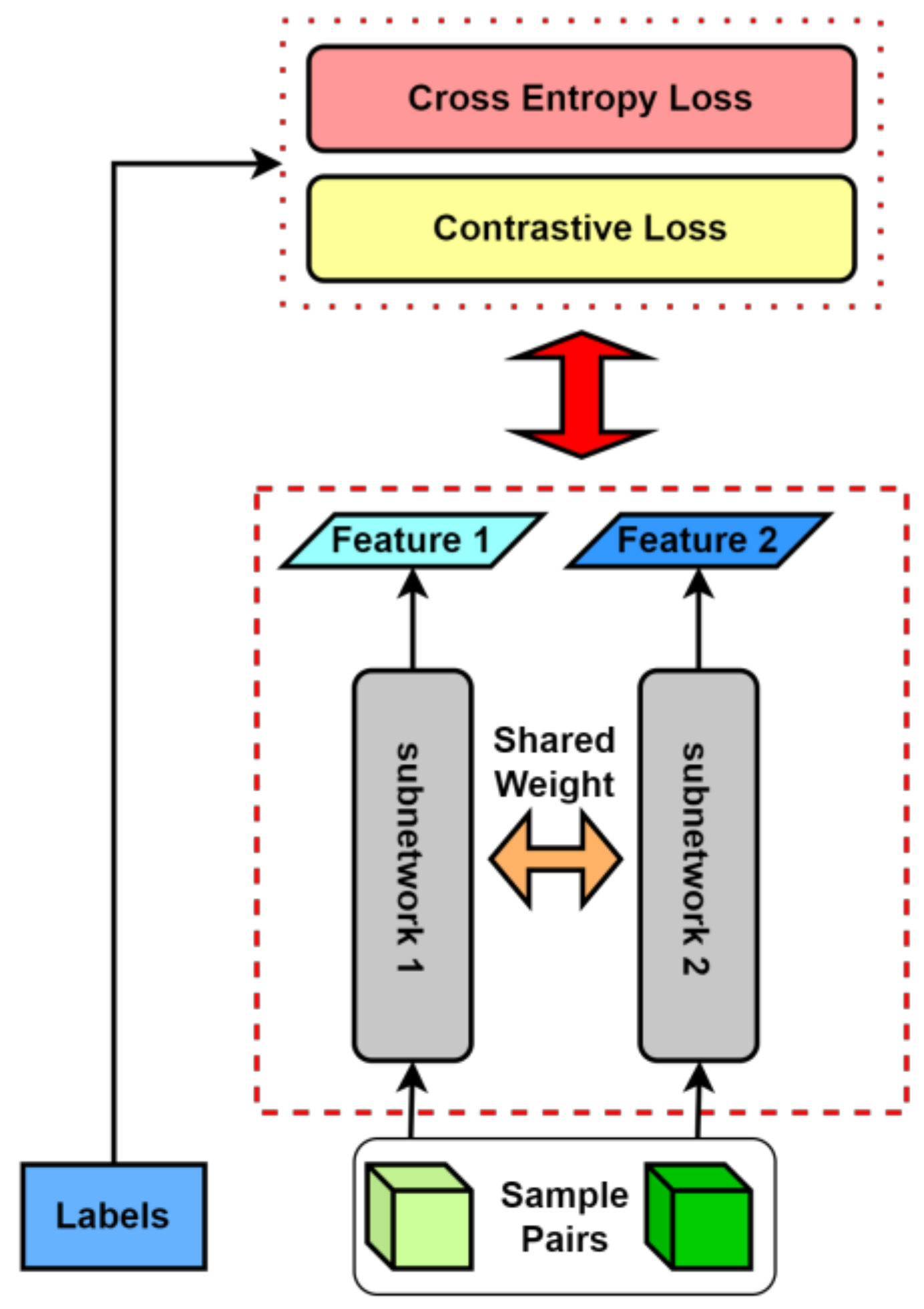
Figure 1.
Structure of a Siamese network.
Figure 1.
Structure of a Siamese network.
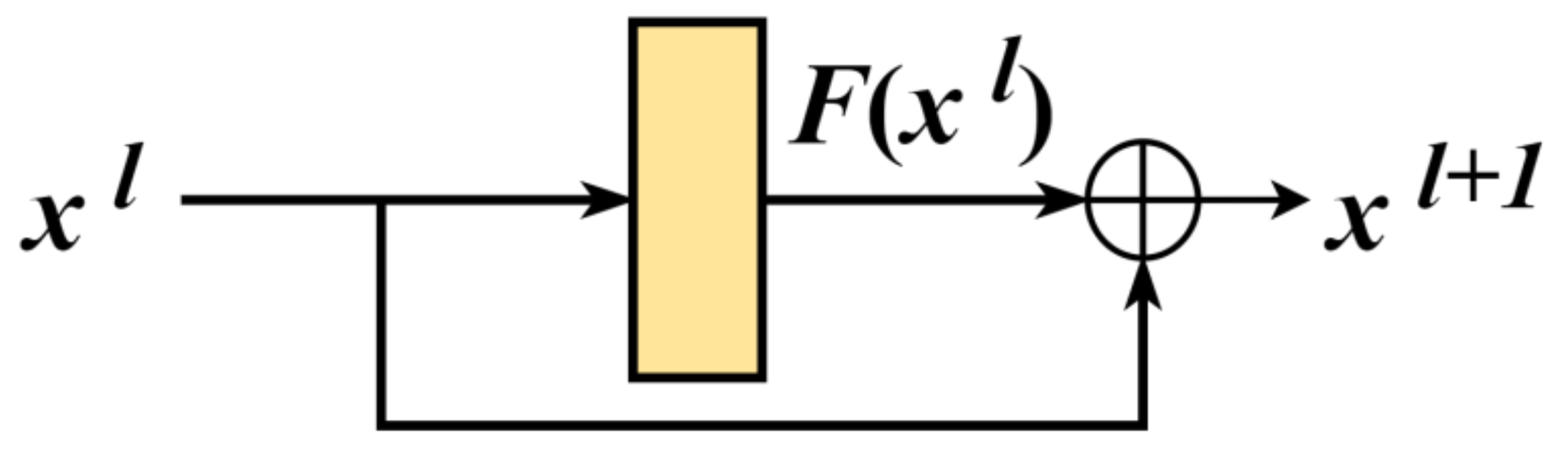
Figure 2.
Residual block.
Figure 2.
Residual block.
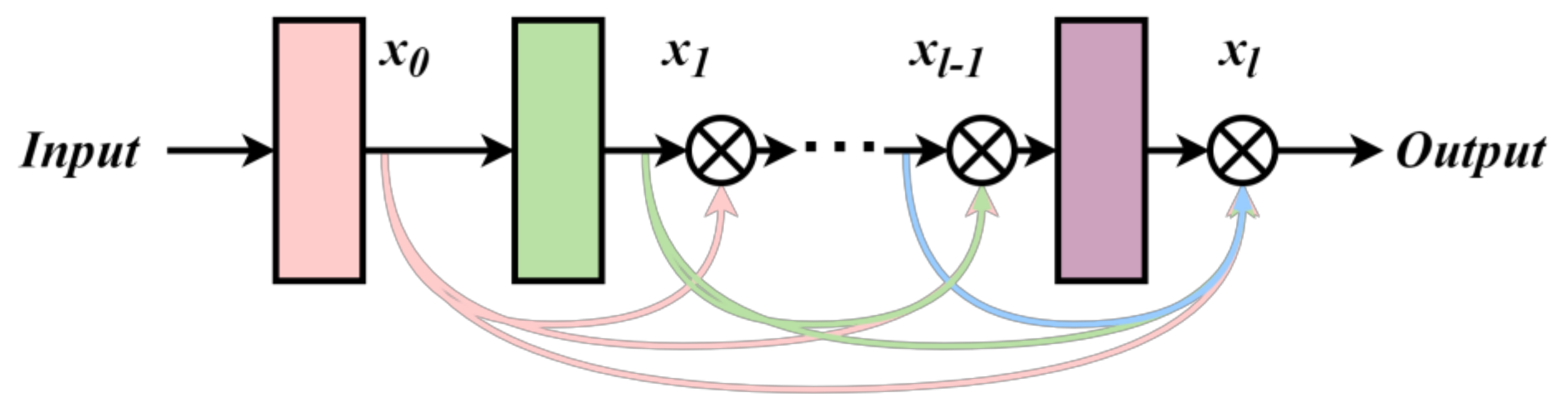
Figure 4.
Architecture of Res2Net.
Figure 4.
Architecture of Res2Net.
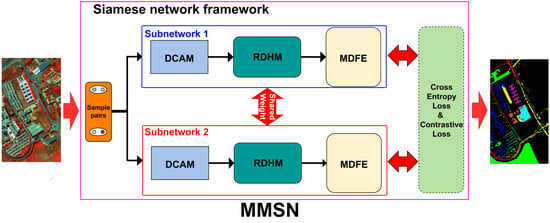
Figure 5.
Flowchart of the proposed MMSN. Two identical Siamese subnetworks consist of DCAM module, RDHM module and MDFE module.
Figure 5.
Flowchart of the proposed MMSN. Two identical Siamese subnetworks consist of DCAM module, RDHM module and MDFE module.
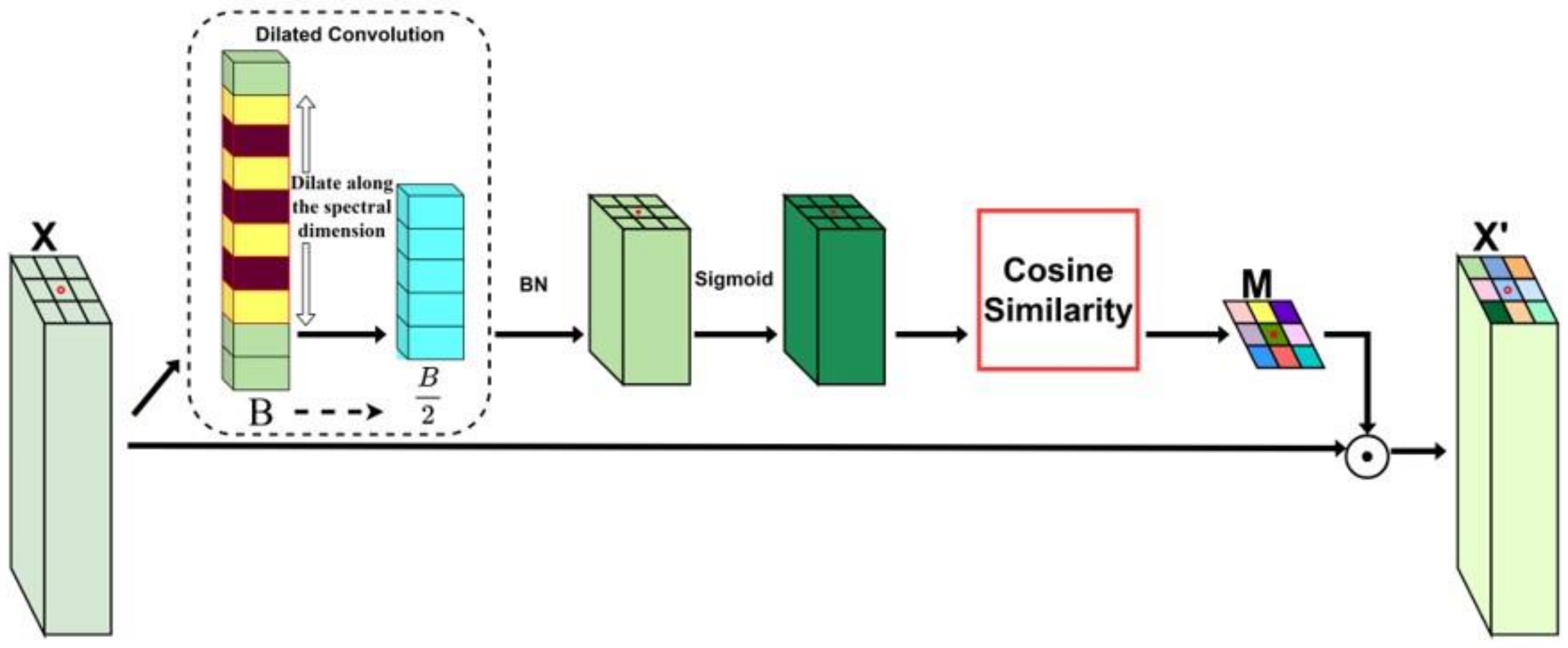
Figure 6.
Diagram of the DCAM. The input patch is X and the weighted output is . B represents the number of channels.
Figure 6.
Diagram of the DCAM. The input patch is X and the weighted output is . B represents the number of channels.
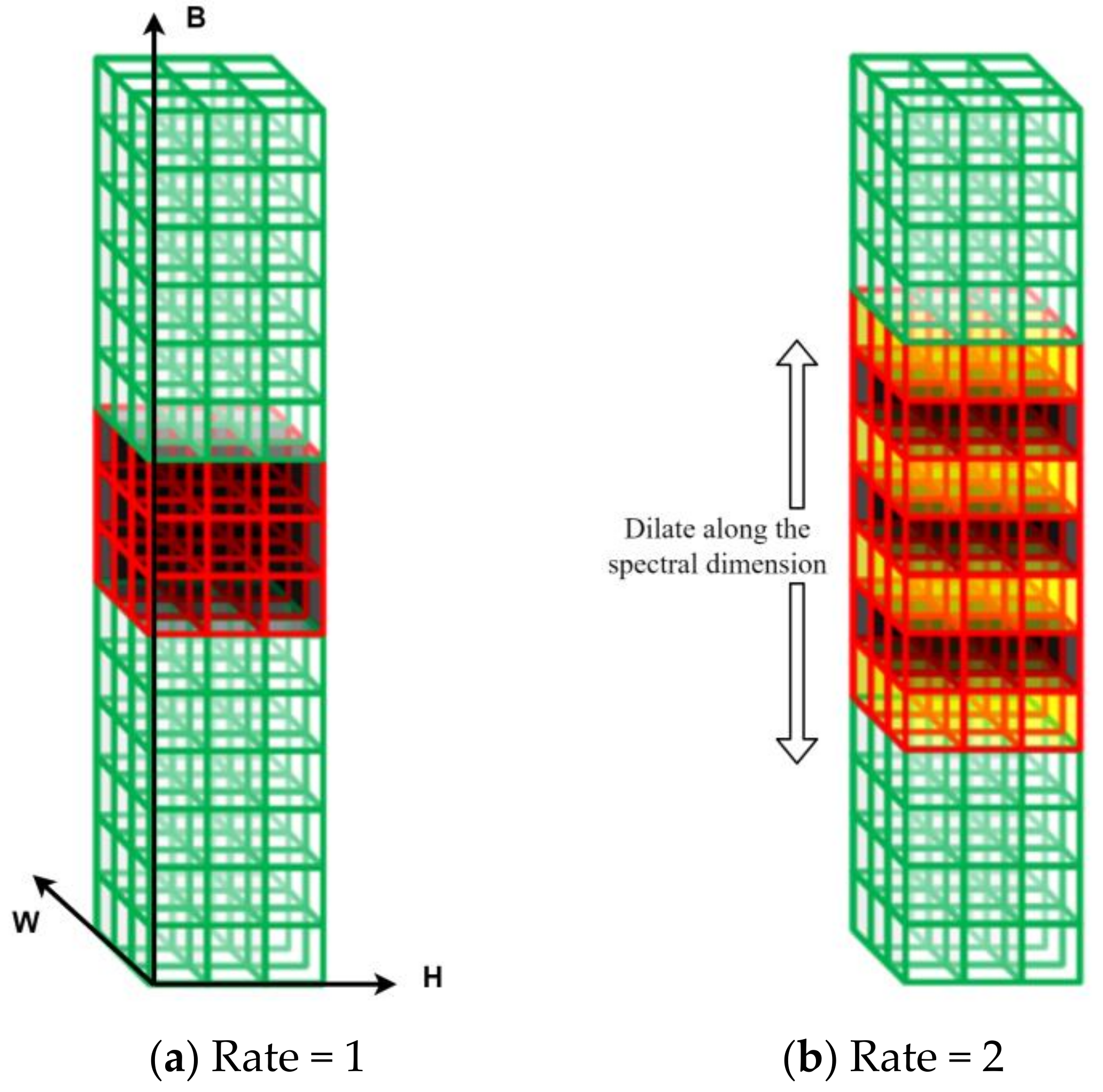
Figure 7.
Illustration of the dilated convolution process. (a) Dilated convolution with dilation rate 1, (b) Dilated convolution with dilation rate 2. The red lines represent the covered receptive field, the black cuboid represents the original convolution kernel, and the yellow part represents the dilated region. B represents the channel dimension, W represents the width dimension, and H represents the height dimension.
Figure 8.
Diagram of the RDHM module. The upper purple branch is global residual branch, the lower black skip branch is global dense branch, and the intermediate blue branch is local residual branch.
Figure 8.
Diagram of the RDHM module. The upper purple branch is global residual branch, the lower black skip branch is global dense branch, and the intermediate blue branch is local residual branch.
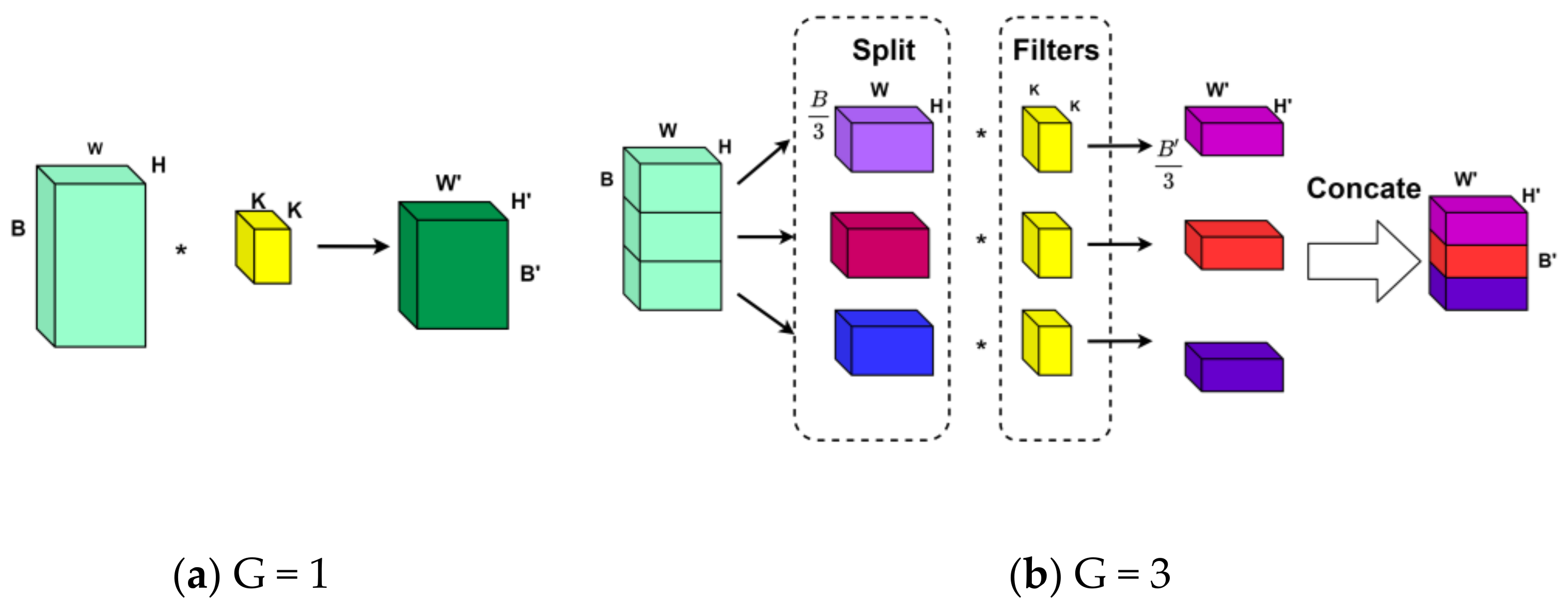
Figure 9.
Illustration of grouped convolution. (a) Grouped convolution with grouped number 1, (b) Grouped convolution with grouped number 3. K represents the size of the convolutional kernel, and “*” represents the convolution operation.
Figure 9.
Illustration of grouped convolution. (a) Grouped convolution with grouped number 1, (b) Grouped convolution with grouped number 3. K represents the size of the convolutional kernel, and “*” represents the convolution operation.
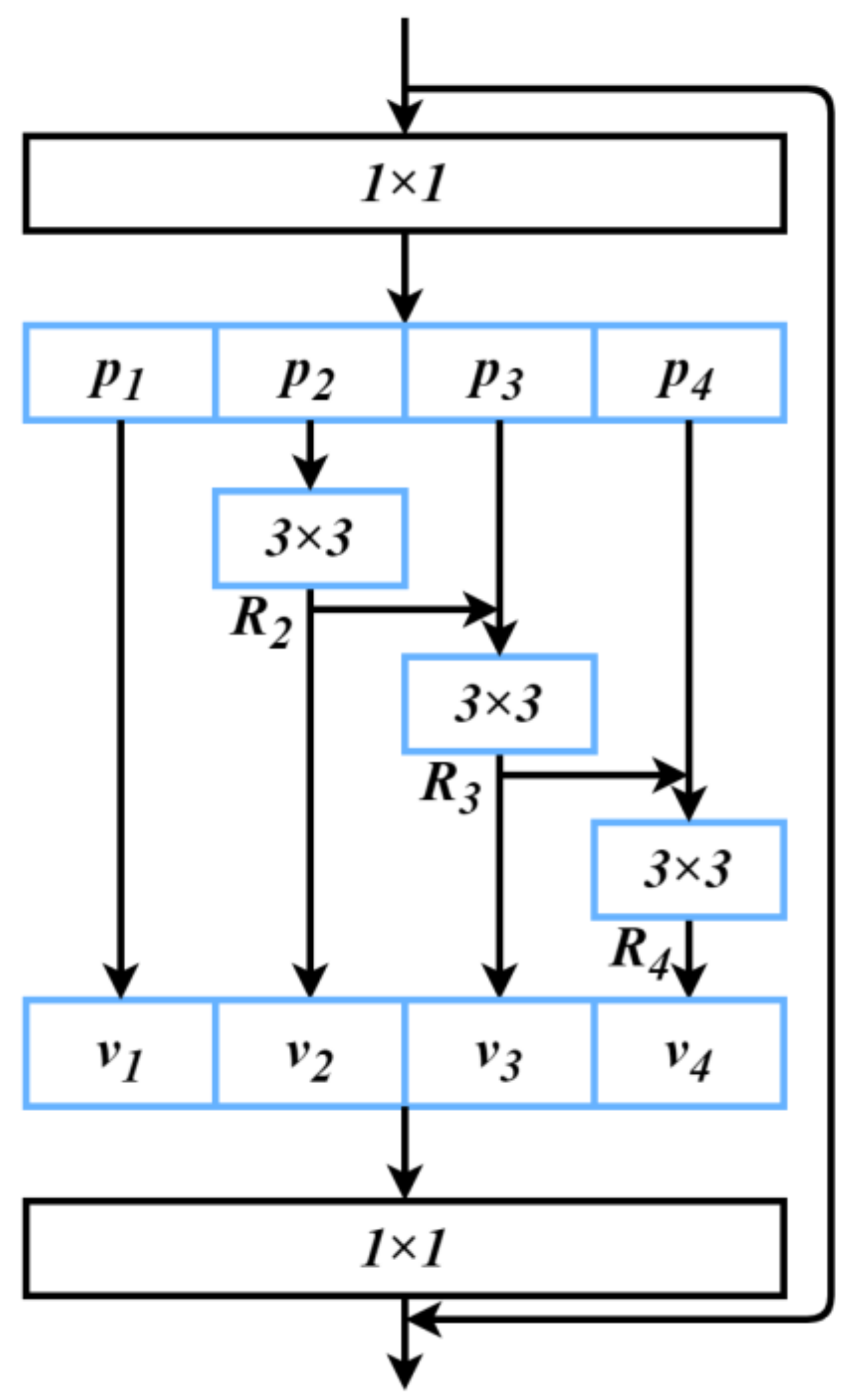
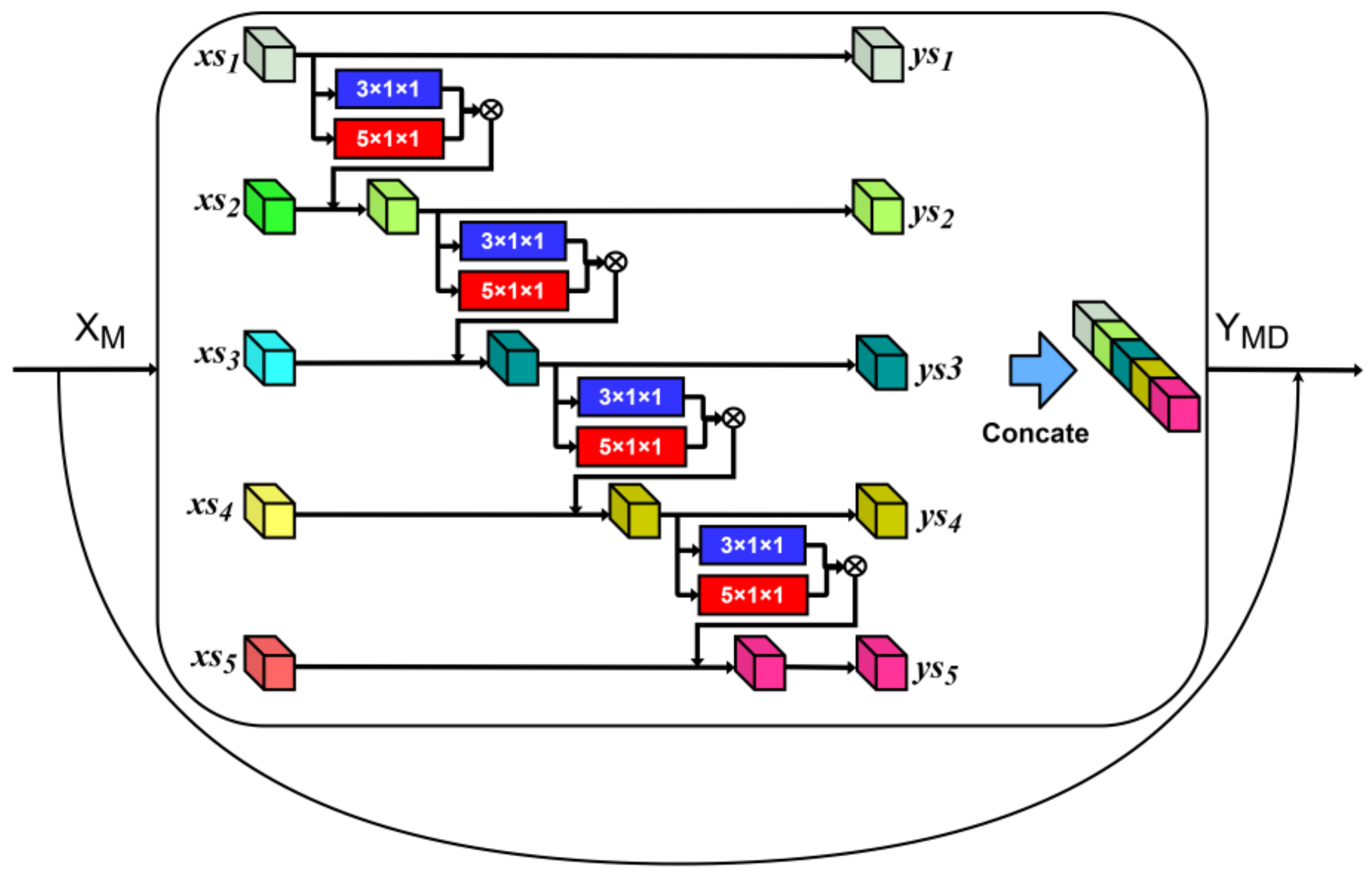
Figure 10.
Diagram of the MDFE module. The input is , the semantic feature output is , and rectangular boxes stand for the multikernels.
Figure 10.
Diagram of the MDFE module. The input is , the semantic feature output is , and rectangular boxes stand for the multikernels.
Figure 11.
A pseudocolor image and ground truth image of PU. (a) The pseudocolor image. (b) The ground truth image.
Figure 11.
A pseudocolor image and ground truth image of PU. (a) The pseudocolor image. (b) The ground truth image.
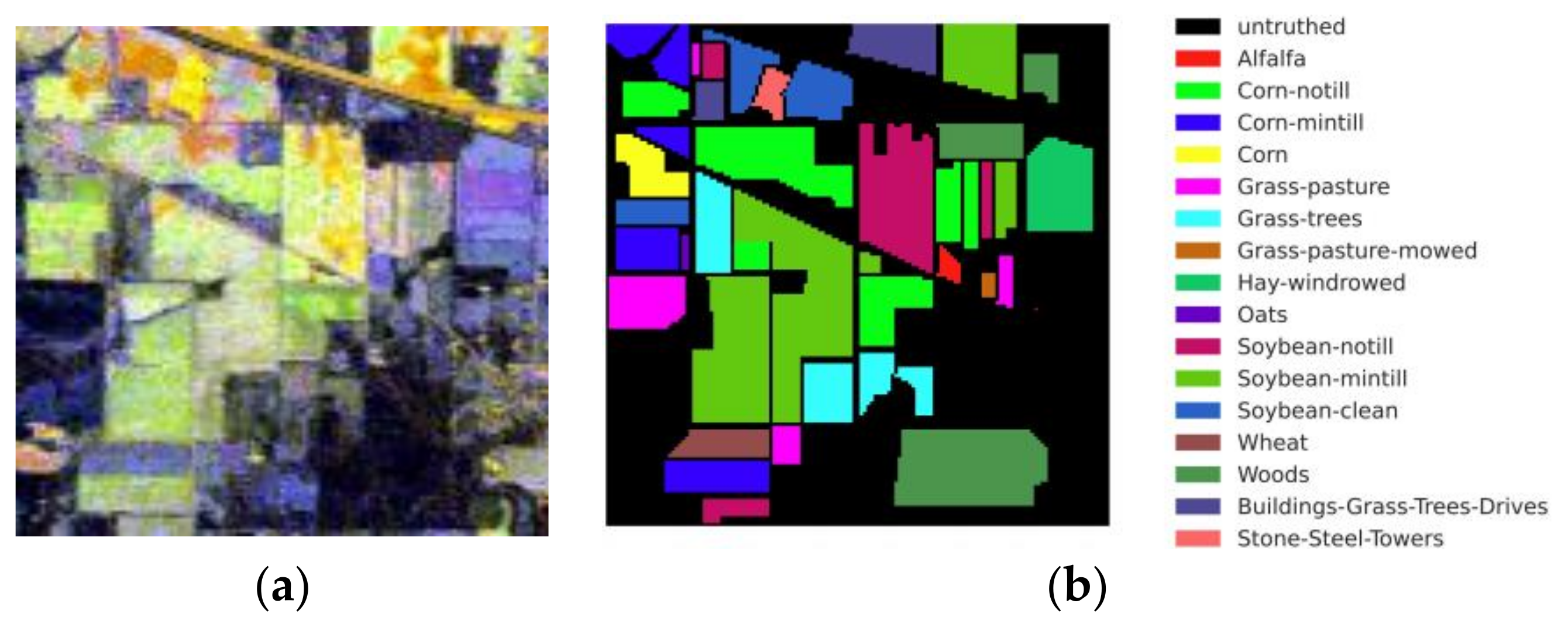
Figure 12.
A pseudocolor image and its corresponding ground truth image of the IP dataset. (a) The pseudocolor image. (b) The ground truth image.
Figure 12.
A pseudocolor image and its corresponding ground truth image of the IP dataset. (a) The pseudocolor image. (b) The ground truth image.
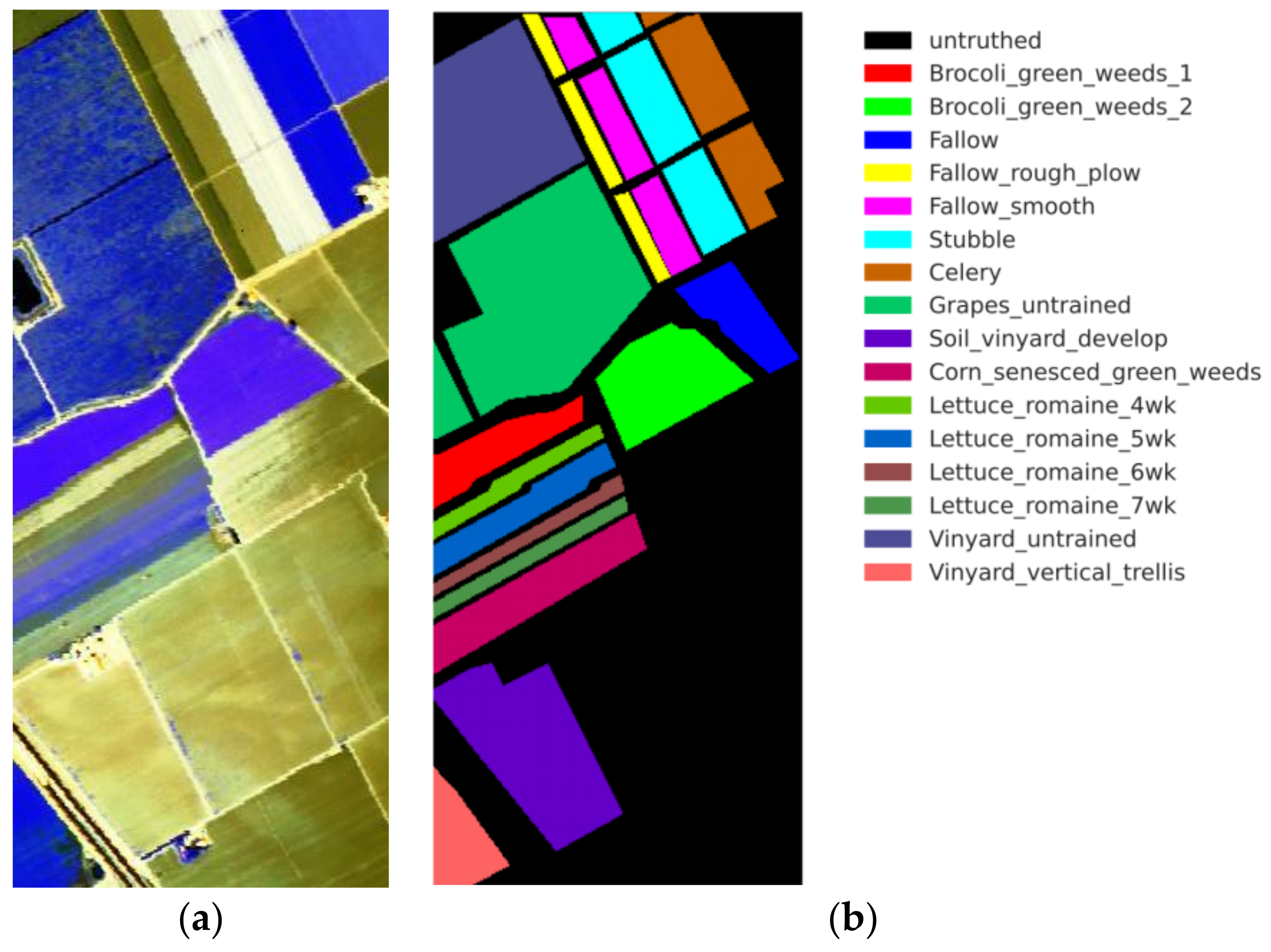
Figure 13.
A pseudocolor image and its corresponding ground truth image of the SA dataset. (a) The pseudocolor image. (b) The ground truth image.
Figure 13.
A pseudocolor image and its corresponding ground truth image of the SA dataset. (a) The pseudocolor image. (b) The ground truth image.
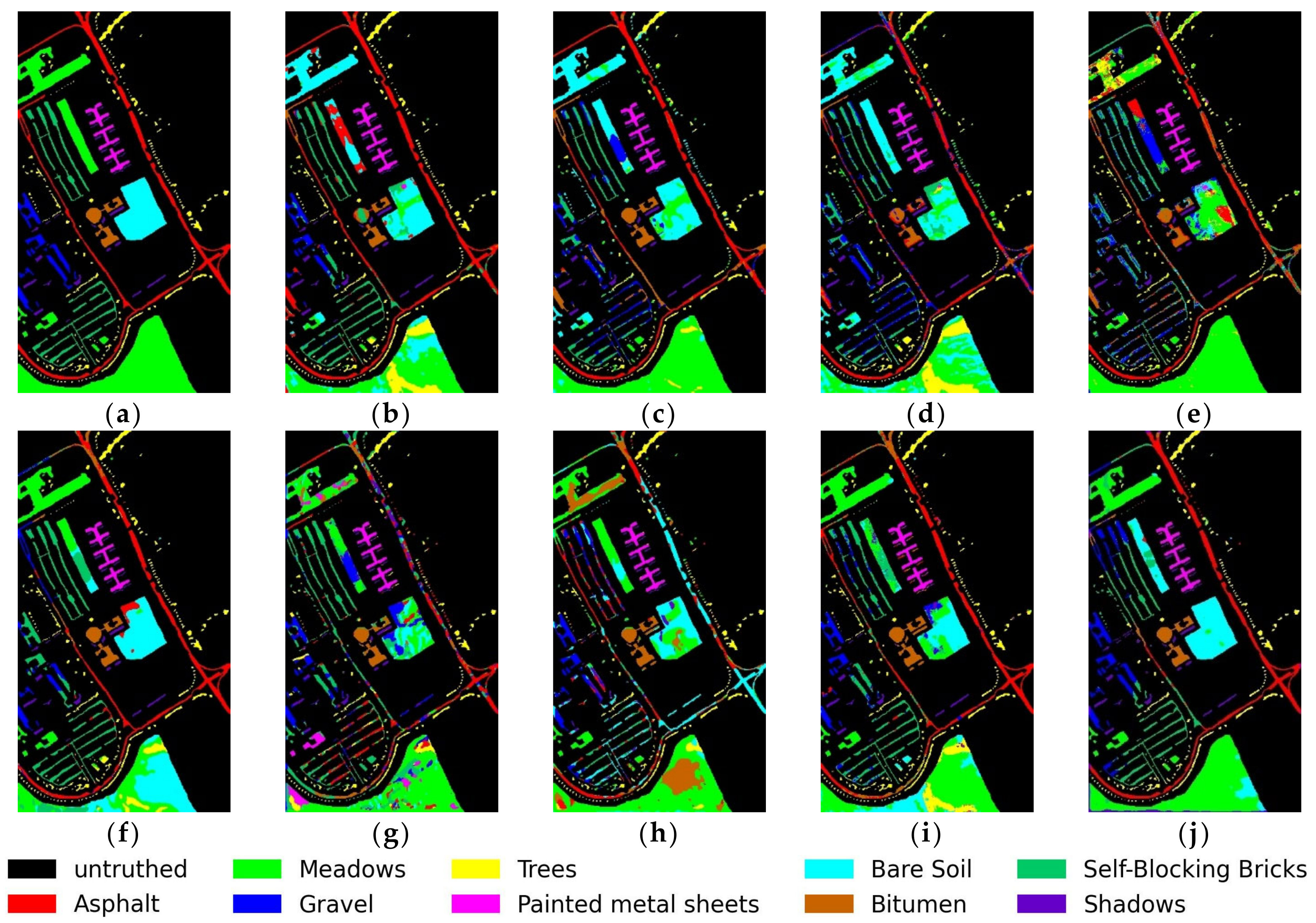
Figure 14.
Classification maps produced for the PU dataset: (a) Ground truth, (b) SSRN (c) FDSSC, (d) DFFN, (e) BASSNet, (f) SPRN, (g) Sia-3DCNN, (h) 3DCSN, (i) S3Net, (j) Proposed MMSN.
Figure 14.
Classification maps produced for the PU dataset: (a) Ground truth, (b) SSRN (c) FDSSC, (d) DFFN, (e) BASSNet, (f) SPRN, (g) Sia-3DCNN, (h) 3DCSN, (i) S3Net, (j) Proposed MMSN.
Figure 15.
Partial enlarged classification maps obtained for the PU dataset: (a) Ground truth, (b) SSRN, (c) FDSSC, (d) DFFN, (e) BASSNet, (f) SPRN, (g) Sia-3DCNN, (h) 3DCSN, (i) S3Net, (j) Proposed MMSN.
Figure 15.
Partial enlarged classification maps obtained for the PU dataset: (a) Ground truth, (b) SSRN, (c) FDSSC, (d) DFFN, (e) BASSNet, (f) SPRN, (g) Sia-3DCNN, (h) 3DCSN, (i) S3Net, (j) Proposed MMSN.
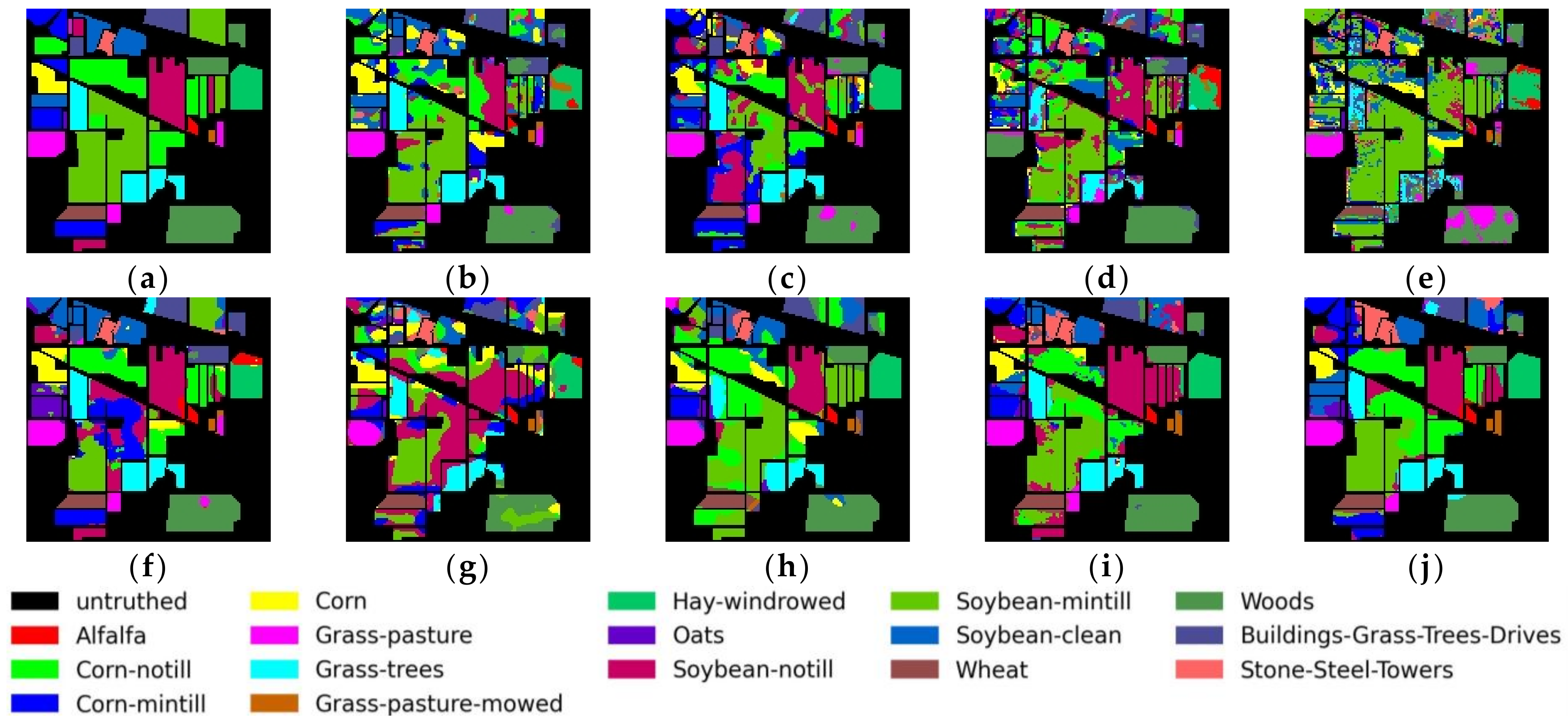
Figure 16.
Classification maps produced for the IP dataset: (a) Ground truth, (b) SSRN, (c) FDSSC, (d) DFFN, (e) BASSNet, (f) SPRN, (g) Sia-3DCNN, (h) 3DCSN, (i) S3Net, (j) Proposed MMSN.
Figure 16.
Classification maps produced for the IP dataset: (a) Ground truth, (b) SSRN, (c) FDSSC, (d) DFFN, (e) BASSNet, (f) SPRN, (g) Sia-3DCNN, (h) 3DCSN, (i) S3Net, (j) Proposed MMSN.
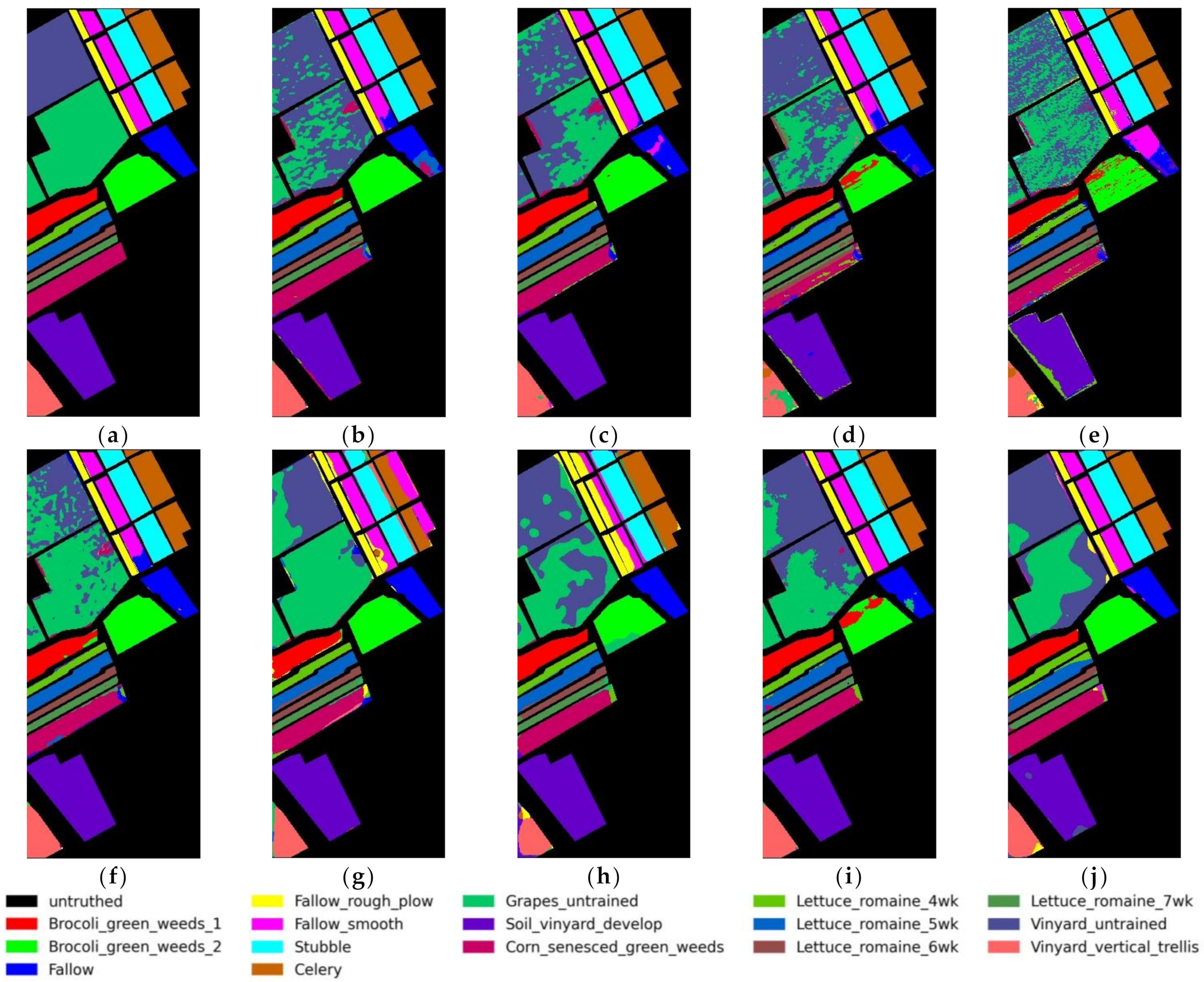
Figure 17.
Classification maps produced for the SA dataset: (a) Ground truth, (b) SSRN, (c) FDSSC, (d) DFFN, (e) BASSNet, (f) SPRN, (g) Sia-3DCNN, (h) 3DCSN (i) S3Net, (j) Proposed MMSN.
Figure 17.
Classification maps produced for the SA dataset: (a) Ground truth, (b) SSRN, (c) FDSSC, (d) DFFN, (e) BASSNet, (f) SPRN, (g) Sia-3DCNN, (h) 3DCSN (i) S3Net, (j) Proposed MMSN.
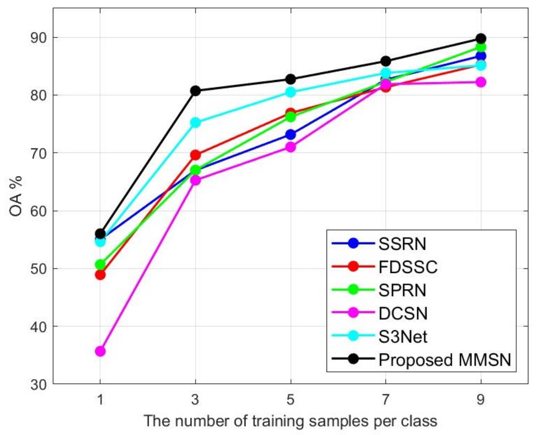
Figure 18.
OA results obtained with different numbers of training samples for PU dataset.
Figure 18.
OA results obtained with different numbers of training samples for PU dataset.
Figure 19.
OA results obtained with different numbers of groups: (a) PU, (b) IP and (c) SA.
Figure 19.
OA results obtained with different numbers of groups: (a) PU, (b) IP and (c) SA.
Figure 20.
OA results obtained with different kernel sizes.
Figure 20.
OA results obtained with different kernel sizes.
Table 1.
The number of samples in each class samples of the PU dataset.
Table 1.
The number of samples in each class samples of the PU dataset.
| Label | Class | #Number |
|---|
| 1 | Asphalt | 6631 |
| 2 | Meadows | 18,649 |
| 3 | Gravel | 2099 |
| 4 | Trees | 3064 |
| 5 | Painted metal sheets | 1345 |
| 6 | Bare Soil | 5029 |
| 7 | Bitumen | 1330 |
| 8 | Self-Blocking Bricks | 3682 |
| 9 | Shadows | 947 |
| Total (9 classes) | 42,776 |
Table 2.
A number of samples of each class samples of the IP dataset.
Table 2.
A number of samples of each class samples of the IP dataset.
| Label | Class | #Number |
|---|
| 1 | Alfalfa | 40 |
| 2 | Corn-notill | 1428 |
| 3 | Corn-mintill | 830 |
| 4 | Corn | 237 |
| 5 | Grass-pasture | 483 |
| 6 | Grass-trees | 730 |
| 7 | Grass-pasture-mowed | 28 |
| 8 | Hay-windrowed | 478 |
| 9 | Oats | 20 |
| 10 | Soybean-notill | 972 |
| 11 | Soybean-mintill | 2455 |
| 12 | Soybean-clean | 593 |
| 13 | Wheat | 205 |
| 14 | Woods | 1265 |
| 15 | Buildings-Grass-Trees-Drives | 386 |
| 16 | Stone-Steel-Towers | 93 |
| Total (16 classes) | 10,249 |
Table 3.
The number of each class samples of the SA dataset.
Table 3.
The number of each class samples of the SA dataset.
| Label | Class | #Number |
|---|
| 1 | Brocoli_green_weeds_1 | 2006 |
| 2 | Brocoli_green_weeds_2 | 3723 |
| 3 | Fallow | 1973 |
| 4 | Fallow_rough_plow | 1391 |
| 5 | Fallow_smooth | 2675 |
| 6 | Stubble | 3956 |
| 7 | Celery | 3576 |
| 8 | Grapes_untrained | 11,268 |
| 9 | Soil_vinyard_develop | 6200 |
| 10 | Corn_senesced_green_weeds | 3275 |
| 11 | Lettuce_romaine_4wk | 1065 |
| 12 | Lettuce_romaine_5wk | 1924 |
| 13 | Lettuce_romaine_6wk | 913 |
| 14 | Lettuce_romaine_7wk | 1067 |
| 15 | Vinyard_untrained | 7265 |
| 16 | Vinyard_vertical_trellis | 1804 |
| Total (16 classes) | 54,081 |
Table 4.
Classification accuracies of different methods for PU dataset (3 training samples per class). The best results are show in bold typeface.
Table 4.
Classification accuracies of different methods for PU dataset (3 training samples per class). The best results are show in bold typeface.
| | SSRN | FDSSC | DFFN | BASSNet | SPRN | Sia-3DCNN | 3DCSN | S3Net | Proposed MMSN |
| OA | 66.99 ± 5.99 | 69.63 ± 8.41 | 52.84 ± 9.08 | 58.55 ± 8.03 | 67.02 ± 7.20 | 63.73 ± 6.19 | 65.27 ± 5.01 | 75.24 ± 6.42 | 80.73 ± 3.87 |
| AA | 81.52 ± 2.34 | 82.94 ± 1.98 | 62.25 ± 6.03 | 64.18 ± 4.10 | 80.99 ± 4.03 | 68.09 ± 4.47 | 71.99 ± 3.08 | 81.75 ± 3.67 | 87.91 ± 2.61 |
| k × 100 | 60.56 ± 5.15 | 63.19 ± 8.64 | 42.69 ± 8.87 | 48.12 ± 8.02 | 60.03 ± 5.56 | 52.65 ± 7.96 | 57.78 ± 6.41 | 68.83 ± 7.18 | 75.86 ± 4.49 |
| Asphalt | 94.16 | 76.82 | 56.21 | 38.61 | 84.63 | 41.46 | 44.01 | 78.82 | 89.64 |
| Meadows | 28.78 | 71.87 | 25.36 | 68.58 | 55.14 | 63.86 | 47.56 | 79.91 | 84.47 |
| Gravel | 49.5 | 65.65 | 38.75 | 48.45 | 65.65 | 97.57 | 93.61 | 68.22 | 97.95 |
| Trees | 82.8 | 92.28 | 65.73 | 91.11 | 97.16 | 83.73 | 88.79 | 98.89 | 68.63 |
| Painted metal sheets | 100 | 100 | 83.12 | 99.25 | 99.93 | 100 | 99.85 | 100 | 100 |
| Bare Soil | 93.07 | 69.02 | 65.54 | 54.67 | 50.73 | 55.15 | 86.69 | 41.34 | 66.19 |
| Bitumen | 99.62 | 97.89 | 84.97 | 82.02 | 92.07 | 92.64 | 92.01 | 99.47 | 100 |
| Self-Blocking Bricks | 87.4 | 45.22 | 23.75 | 56.99 | 80.41 | 53.57 | 46.91 | 91.91 | 97.65 |
Table 5.
Classification accuracies of different methods on the IP dataset (3 training samples per class). The best results are show in bold typeface.
Table 5.
Classification accuracies of different methods on the IP dataset (3 training samples per class). The best results are show in bold typeface.
| | SSRN | FDSSC | DFFN | BASSNet | SPRN | Sia-3DCNN | 3DCSN | S3Net | Proposed MMSN |
| OA | 58.76 ± 6.51 | 53.81 ± 4.21 | 41.04 ± 5.97 | 42.96 ± 4.16 | 69.27 ± 6.98 | 50.34 ± 2.81 | 59.62 ± 3.20 | 66.66 ± 1.88 | 72.82 ± 2.71 |
| AA | 74.07 ± 5.04 | 70.93 ± 3.09 | 53.97 ± 3.02 | 52.36 ± 3.24 | 79.37 ± 3.59 | 64.84 ± 3.49 | 74.33 ± 2.47 | 79.66 ± 2.35 | 82.64 ± 1.23 |
| k × 100 | 54.01 ± 7.04 | 49.39 ± 4.35 | 34.41 ± 5.98 | 36.23 ± 4.29 | 60.03 ± 5.56 | 44.68 ± 2.94 | 54.83 ± 3.49 | 62.85 ± 2.05 | 69.61 ± 1.83 |
| Alfalfa | 100 | 65.01 | 50.02 | 57.51 | 95.01 | 100 | 100 | 100 | 100 |
| Corn-notill | 56.68 | 27.43 | 29.04 | 5.84 | 61.11 | 50.73 | 25.12 | 64.99 | 61.68 |
| Corn-mintill | 75.85 | 52.55 | 18.08 | 8.01 | 61.77 | 31.21 | 54.17 | 47.59 | 42.93 |
| Corn | 95.67 | 97.4 | 2.03 | 29.44 | 64.94 | 64.1 | 82.48 | 68.35 | 86.32 |
| Grass-pasture | 63.31 | 80.92 | 71.28 | 59.96 | 83.44 | 66.88 | 68.13 | 84.6 | 62.51 |
| Grass-trees | 55.39 | 89.23 | 36.6 | 40.06 | 96.15 | 87.62 | 91.75 | 92.33 | 98.34 |
| Grass-pasture-mowed | 100 | 100 | 86.36 | 72.73 | 100 | 72 | 100 | 100 | 100 |
| Hay-windrowed | 58.69 | 59.53 | 62.08 | 73.31 | 99.58 | 88.21 | 89.68 | 98.74 | 100 |
| Oats | 100 | 100 | 92.86 | 100 | 100 | 100 | 100 | 100 | 100 |
| Soybean-notill | 15.22 | 51.66 | 29.61 | 16.46 | 63.98 | 25.28 | 61.71 | 82.41 | 84.62 |
| Soybean-mintill | 36.3 | 31.03 | 30.3 | 73.17 | 10.62 | 47.92 | 41.11 | 36.86 | 69.21 |
| Soybean-clean | 51.11 | 34.24 | 16.01 | 23.34 | 67.97 | 36.61 | 46.61 | 76.05 | 86.11 |
| Wheat | 94.97 | 96.48 | 81.41 | 67.34 | 100 | 86.14 | 96.53 | 100 | 100 |
| Woods | 93.96 | 65.05 | 63.54 | 69.98 | 50.36 | 64.18 | 87.71 | 97.78 | 96.99 |
| Buildings-Grass-Trees-Drives | 66.05 | 62.37 | 57.63 | 23.95 | 69.47 | 56.91 | 22.45 | 53.88 | 73.89 |
Table 6.
Classification accuracies of different methods for SA dataset (3 training samples per class). The best results are show in bold typeface.
Table 6.
Classification accuracies of different methods for SA dataset (3 training samples per class). The best results are show in bold typeface.
| | SSRN | FDSSC | DFFN | BASSNet | SPRN | Sia-3DCNN | 3DCSN | S3Net | Proposed MMSN |
| OA | 83.72 ± 3.52 | 83.03 ± 3.82 | 76.58 ± 2.85 | 75.66 ± 3.17 | 87.59 ± 3.42 | 85.62 ± 2.07 | 88.20 ± 1.97 | 88.84 ± 3.21 | 90.81 ± 1.59 |
| AA | 89.87 ± 2.7 | 89.84 ± 2.38 | 82.98 ± 3.14 | 81.24 ± 3.81 | 92.94 ± 2.14 | 88.55 ± 2.05 | 91.44 ± 1.48 | 92.39 ± 1.24 | 93.78 ± 0.91 |
| k × 100 | 89.91 ± 3.89 | 81.20 ± 4.36 | 74.14 ± 3.19 | 72.91 ± 3.56 | 86.23 ± 3.84 | 84.02 ± 2.27 | 86.90 ± 2.16 | 87.62 ± 3.53 | 89.77 ± 1.75 |
| Brocoli_green_weeds_1 | 98.45 | 100 | 85.87 | 99.25 | 99.95 | 92.57 | 99.6 | 100 | 100 |
| Brocoli_green_weeds_2 | 99.73 | 99.84 | 95.03 | 95.7 | 99.76 | 99.54 | 98.58 | 83.81 | 100 |
| Fallow | 67.06 | 90.36 | 55.38 | 71.78 | 75.69 | 99.54 | 98.73 | 93.76 | 100 |
| Fallow_rough_plow | 99.42 | 98.13 | 99.14 | 98.41 | 100 | 100 | 94.03 | 99.07 | 99.64 |
| Fallow_smooth | 89.22 | 96.29 | 60.89 | 90.61 | 97.53 | 65.64 | 99.14 | 99.96 | 86.54 |
| Stubble | 99.75 | 99.92 | 96.13 | 96.23 | 99.77 | 78.76 | 96.74 | 95.73 | 100 |
| Celery | 99.75 | 99.94 | 94.6 | 97.9 | 99.97 | 65.91 | 99.77 | 100 | 99.94 |
| Grapes_untrained | 44.46 | 49.52 | 62.86 | 27.72 | 35.2 | 91.59 | 78.27 | 61.43 | 47.99 |
| Soil_vinyard_develop | 97.21 | 99.98 | 82.51 | 94.26 | 98.03 | 99.88 | 100 | 100 | 100 |
| Corn_senesced_green_weeds | 92.45 | 90.07 | 27.84 | 62.93 | 32.95 | 77.01 | 92.67 | 94.05 | 93.92 |
| Lettuce_romaine_4wk | 90.58 | 94.92 | 96.23 | 58.57 | 99.91 | 100 | 100 | 100 | 42.35 |
| Lettuce_romaine_5wk | 100 | 99.95 | 99.64 | 99.32 | 100 | 89.03 | 91.21 | 94.29 | 71.88 |
| Lettuce_romaine_6wk | 99.89 | 99.67 | 98.9 | 99.23 | 100 | 99.34 | 99.45 | 82.09 | 100 |
| Lettuce_romaine_7wk | 94.27 | 98.31 | 96.52 | 94.08 | 98.03 | 92.59 | 95.51 | 98.03 | 81.63 |
| Vinyard_untrained | 89.36 | 77.71 | 78.86 | 89.37 | 89.73 | 67.66 | 83.05 | 80.99 | 97.49 |
Table 7.
Impacts of different modules on the PU dataset. Y means that the corresponding module is used; N means that the corresponding module is not used.
Table 7.
Impacts of different modules on the PU dataset. Y means that the corresponding module is used; N means that the corresponding module is not used.
| Siamese | DCAM | RDHM | MDFE | OA (%) |
|---|
| Y | Y | Y | Y | 80.73 |
| N | Y | Y | Y | 66.61 |
| Y | Y | N | Y | 51.44 |
| Y | Y | Y | N | 67.92 |
| Y | N | Y | Y | 64.97 |


