Hybrid Convolutional Network Combining Multiscale 3D Depthwise Separable Convolution and CBAM Residual Dilated Convolution for Hyperspectral Image Classification

Abstract

In recent years, convolutional neural networks (CNNs) have been increasingly leveraged for the classification of hyperspectral imagery, displaying notable advancements. To address the issues of insufficient spectral and spatial information extraction and high computational complexity in hyperspectral image classification, we introduce the MDRDNet, an integrated neural network model. This novel architecture is comprised of two main components: a Multiscale 3D Depthwise Separable Convolutional Network and a CBAM-augmented Residual Dilated Convolutional Network. The first component employs depthwise separable convolutions in a 3D setting to efficiently capture spatial–spectral characteristics, thus substantially reducing the computational burden associated with 3D convolutions. Meanwhile, the second component enhances the network by integrating the Convolutional Block Attention Module (CBAM) with dilated convolutions via residual connections, effectively counteracting the issue of model degradation. We have empirically evaluated the MDRDNet’s performance by running comprehensive experiments on three publicly available datasets: Indian Pines, Pavia University, and Salinas. Our findings indicate that the overall accuracy of the MDRDNet on the three datasets reached 98.83%, 99.81%, and 99.99%, respectively, which is higher than the accuracy of existing models. Therefore, the MDRDNet proposed in this study can fully extract spatial–spectral joint information, providing a new idea for solving the problem of large model calculations in 3D convolutions.

1. Introduction

Hyperspectral imagery (HSIs) represents a unique category of images captured using advanced sensors tailored to gather data across a continuous and broad spectral range. Each pixel in an HSI carries a distinctive signature spanning multiple spectral bands [1]. Owing to their data richness, HSIs find utility in diverse fields such as agricultural monitoring [2], ecological assessments [3], mineral detection [4], medical diagnostics [5], and military tactics [6]. With hyperspectral image classification (HSIC) gaining prominence in remote sensing research, the precise interpretation and correct analysis of both the spatial and spectral components of these images have become paramount [7].

In the initial stages of HSIC, the focus was primarily on spectral feature-based techniques. Key methods encompassed Support Vector Machines (SVM) [8], a Random Forest (RF) [9], and k-Nearest Neighbors (KNN) [10]. Although these conventional algorithms possess certain advantages, they often overlook spatial characteristics, yielding classification outcomes that do not consistently meet practical requirements. A compounding challenge is that HSIs frequently demonstrate substantial variation within a class while presenting considerable resemblance among distinct classes. For instance, external environmental variables might cause shifts in the spectral signatures of consistent ground entities. Conversely, unrelated terrestrial groups might share similar spectral patterns, especially when contamination exists between neighboring areas, complicating accurate object classification [11]. Hence, an excessive reliance on merely spectral characteristics is likely to result in the misclassification of the intended subjects [12].

In recent years, hyperspectral image classification (HSIC) has benefitted from the integration of deep learning algorithms, noted for their outstanding feature extraction prowess [13]. Convolutional neural networks (CNNs), in particular, have established themselves as a dominant approach within this field [14]. Initial endeavors, exemplified by the study of Hu et al., utilized a one-dimensional CNN to transform each pixel in the hyperspectral image into a 1D vector, aiming for spectral feature extraction [15]. In a similar vein, Cao et al. harnessed a two-dimensional CNN in conjunction with Markov Random Fields to amalgamate spatial and spectral data, thus augmenting classification accuracy [16]. Zhao et al. incorporated Principal Component Analysis (PCA) for dimensionality reduction, followed by the application of a 2D-CNN for spatial feature extraction from hyperspectral images [17]. However, while these studies primarily employ 1D and 2D CNN architectures, they face inherent constraints. Namely, 1D CNNs present simplicity issues, whereas 2D CNNs do not fully exploit both spatial and spectral features, creating impediments to potential enhancements in HSIC accuracy [18].

Three-dimensional Convolutional Neural Networks (3D-CNNs) have become instrumental in extracting both spatial and spectral features concurrently, enhancing the precision of hyperspectral image classification (HSIC). Zhang et al. proposed a unique architecture incorporating parallel 3D Inception layers. This model leverages cross-entropy-based dimensionality reduction techniques to adaptively select spectral bands, thus refining classification results [19]. Similarly, Zhang et al. introduced the End-to-End Spectral Spatial Residual Network (SSRN), a design that integrates 3D-CNN layers within a residual network structure. It employs dual consecutive residual blocks to independently learn spatial and spectral features, confirming the efficacy of dual-dimension feature learning in refining classification precision [20]. Additionally, Roy et al. crafted a network architecture named HybridSN, which sequences three 3D-CNN layers for initial feature fusion and subsequent 2D-CNN layers for spatial feature extraction, highlighting the benefits of mixed convolutional dimensions in HSIC contexts [21].

Despite the precision of 3D-CNN-based classifications, they are often associated with considerable computational demands, especially during fully connected mapping stages, attributable to the extensive parameter generation [22]. Addressing this, Howard et al. substituted 2D-CNN layers in their design with depthwise separable convolutions, significantly reducing parameter counts during convolutional operations [23]. Similarly, Zhao et al. incorporated depthwise separable convolutions into a multi-residual framework to balance computational efficiency with classification accuracy [22]. Wang et al. developed a resource-optimized convolutional model, blending rapid 3D-CNN algorithms with depthwise separable convolutions, facilitating spatial–spectral feature extraction without parameter escalation [24]. A subsequent analysis indicated the superior descriptive capacity of multi-scale features for the intricacies of HSIs. Thus, integrating features across various scales can elevate classification performance [25]. Correspondingly, Shi et al. conceptualized a dual-branch, multi-scale spectral attention network utilizing diverse convolutional kernel sizes to extract features over multiple scales [26]. Gong et al. devised a Hybrid 2D-3D CNN Multi-Scale Information Fusion Network (MSPN) to deepen network structures vertically and expand multi-scale spatial and spectral data horizontally [27]. Wang et al. also introduced the Multi-Scale Dense Connection Attention Network (MSDAN) adept at capturing variegated features from HSIs across different scales, mitigating issues such as model overfitting and gradient disappearance [28].

The attention mechanism has recently gained significant traction in computer vision, paving the way for enhanced feature extraction [29]. Fang et al. introduced a 3D Dense Convolutional Network, fortified with a spectral attention mechanism. This network utilizes 3D dilated convolutions to apprehend spatial and spectral features across various scales. Moreover, spectral attention is employed to enhance the discriminative capabilities of high-spectral images (HSIs) [30]. Adding to the body of work on attention mechanisms, Li et al. presented the Dual-Branch Double-Attention Mechanism Network (DBDA). This innovative model introduces self-attention in both spectral and spatial dimensions, thus augmenting the capacity of images to articulate nuanced details [31]. Liu’s team, on the other hand, designed a Modified Dense Attention Network (MDAN) specifically for Hyperspectral Image Classification (HSIC). Their model incorporates a Convolutional Block Self-Attention Module (CBSM), which is an adaptation of the Convolutional Block Attention Module (CBAM), and improves classification performance by refining the connection patterns among attention blocks [32].

The existing literature underscores that while 3D convolution excels in spatial–spectral feature extraction, it induces significant computational overhead. Further, the integration of multi-scale features and attention mechanisms markedly enhances classification model performance. Given these insights, this study presents an end-to-end hybrid convolutional network, comprising both 2D-CNN and 3D-CNN modules, tailored for Hyperspectral Image Classification (HSIC). Within this framework, the 3D-CNN modules adeptly discern spatial–spectral features across diverse scales, and the 2D-CNN modules accentuate spatial characteristics.

The paper makes the following contributions:

• We employ a multi-scale convolutional fusion technique within the 3D-CNN module, enhancing the comprehensive extraction of hyperspectral image features in both the spatial and spectral domains.
• Replacing standard 3D convolutional layers with 3D depth separable convolutional layers, we optimize training efficiency and mitigate the risk of overfitting, while maintaining high classification accuracy.
• Incorporating the Convolutional Block Attention Module (CBAM) within the residual network architecture, we substitute standard 2D convolutional layers with dilated versions, thus expanding the receptive field and boosting feature extraction for ground object identification.

The subsequent sections of this manuscript are structured in the following manner: Section 2 explores the intricacies of the MDRDNet’s design and its associated features; in Section 3, we shed light on the results of the experiments conducted; in Section 4, we engage in a discussion regarding their implications; and finally, Section 5 serves to wrap up the findings and conclusion of this paper.

2. Methods

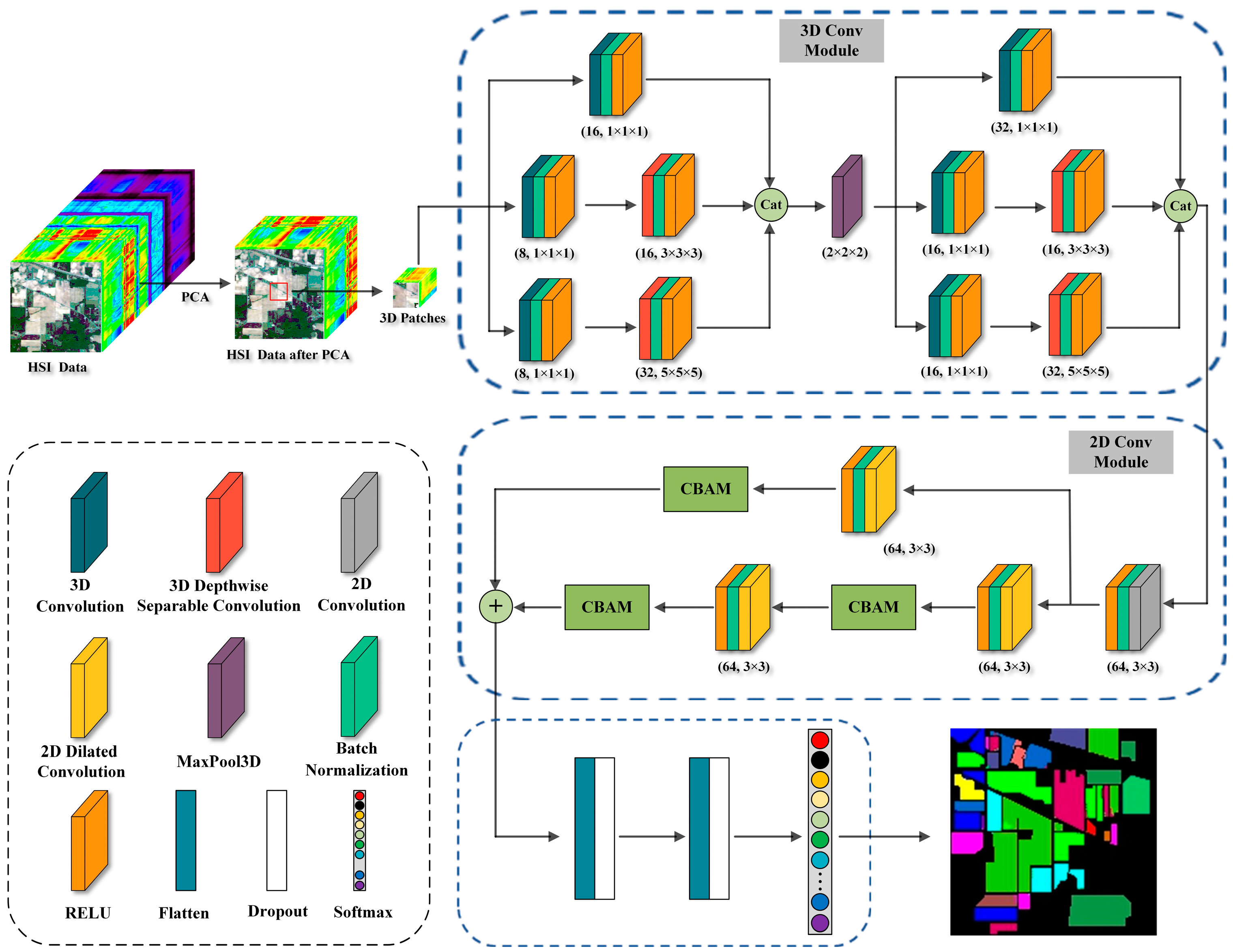
Figure 1 delineates the configuration of MDRDNet, which has been tailored for this research. To commence, the high-dimensional hyperspectral image data are first subjected to Principal Component Analysis (PCA) to curtail dimensionality while lessening spectral redundancy. Following this dimensionality reduction, the image is further segmented into neighborhood-based 3D blocks. In the next step, a multi-scale 3D convolutional network, characterized by depthwise separable 3D convolutions, is utilized to extract both spatial and spectral features. Afterward, the convolutional outputs are reshaped and directed through a Convolutional Block Attention Module (CBAM) that is integrated into a residual network and enhanced with dilated convolutions. The classification procedure culminates with the data, traversing a series of two fully connected layers before entering a Softmax activation layer for final categorization.

2.1. Processing of Raw Data

Hyperspectral images (HSIs) possess inherent complexity due to their multi-band spectral richness. A single pixel often exhibits inter-band correlations, giving rise to a level of redundancy in the information captured. Such an overload of information can muddle the training algorithms of machine learning models [33]. To address this challenge, Figure 2 shows our initial step: the implementation of Principal Component Analysis (PCA) to simplify the spectral information while maintaining the essential spatial features of the images. Let the dimensions of the original HSI be denoted as $I\in A^H{}^{\times W\times C}$, with I representing the input data, H and W symbolizing the height and width of this data, respectively, and C standing for the total number of spectral bands. Post-PCA, the image is resized to dimensions $X\in A^H{}^{\times W\times B}$, where X is the dimension-reduced data cube and B is the reduced number of bands. Relying solely on spectral data for classifying HSIs can impair the model’s performance, given that such an approach would exclude a wealth of spatial information. Consequently, after reducing the dimensions through PCA, we extract localized neighborhoods from the images. We treat the pixels within these neighborhoods as individual samples to incorporate supplemental spatial data. The data cube X is subsequently segmented into overlapping 3D blocks denoted as $P\in A^S{}^{\times S\times B}$, where P signifies the partitioned data cube, B the number of bands, and S the dimensions (height and width) of P.

2.2. Three-Dimensional Convolution Module

2.2.1. Three-Dimensional Depthwise Separable Convolution

In 2017, Howard and collaborators unveiled MobilenetV1, a streamlined network architecture that employs depthwise separable convolutions. This architecture optimizes both computational efficiency and performance, making it particularly suitable for mobile and embedded devices. One of the key advantages of utilizing depthwise separable convolutions lies in their computational lightness. These convolutions break down a full-fledged convolutional operation into two distinct phases. Initially, depthwise convolution is carried out, handling each channel of the input layer independently. Subsequently, pointwise convolution merges the channel-wise weighted feature maps generated in the prior step to produce new composite feature maps.

Depthwise separable convolutions are advantageous over classic convolutional layers as they necessitate a smaller number of parameters and have lower computational demand. For a conventional convolutional layer, the parameters can be depicted as D_k × D_k × M × N, where D_k represents the 2D convolutional kernel dimensions, M is the number of input channels, and N signifies the output channels. With appropriate padding, the input feature map dimensions are represented as D_F × D_G × M, where D_F and D_G are the height and width of the input, respectively. We denote the computational complexity of a standard 2D convolution as Cost_A, calculated as follows:

$${\mathrm{Cost}}_{\mathrm{A}}={\mathrm{D}}_{\mathrm{K}}·{\mathrm{D}}_{\mathrm{K}}·\mathrm{M}·\mathrm{N}·{\mathrm{D}}_{\mathrm{F}}·{\mathrm{D}}_{\mathrm{G}}.$$

(1)

In the context of 2D depthwise separable convolution, the associated computational cost is denoted as Cost_DW. Specifically, Cost_D and Cost_P represent the computational expenses for the depthwise and pointwise convolutions, respectively, within this specialized convolution operation. It should be noted that the computational demands for depthwise convolution parallel those of a standard convolution kernel. The ability to generate multiple output channels is conferred by the subsequent pointwise convolution, which has a kernel size of 1. Considering the employment of N of such convolutional kernels, we can express Cost_DW through the following calculation:

$$\begin{array}{cc}\hfill {\mathrm{Cost}}_{\mathrm{D}\mathrm{W}}& ={\mathrm{Cost}}_{\mathrm{D}}+{\mathrm{Cost}}_{\mathrm{P}},\hfill \\ & ={\mathrm{D}}_{\mathrm{K}}·{\mathrm{D}}_{\mathrm{K}}·\mathrm{M}·{\mathrm{D}}_{\mathrm{F}}·{\mathrm{D}}_{\mathrm{G}}+\mathrm{M}·\mathrm{N}·{\mathrm{D}}_{\mathrm{F}}·{\mathrm{D}}_{\mathrm{G}}.\hfill \end{array}$$

(2)

To evaluate the computational load differences between a conventional 2D convolution and a 2D depthwise separable convolution, one can express the computational efficiency ratio as delineated below:

$$\begin{array}{cc}\hfill \frac{{\mathrm{Cost}}_{\mathrm{D}\mathrm{W}}}{{\mathrm{Cost}}_{\mathrm{A}}}& =\frac{{\mathrm{D}}_{\mathrm{K}}·{\mathrm{D}}_{\mathrm{K}}·\mathrm{M}·{\mathrm{D}}_{\mathrm{F}}·{\mathrm{D}}_{\mathrm{G}}+\mathrm{M}·\mathrm{N}·{\mathrm{D}}_{\mathrm{F}}·{\mathrm{D}}_{\mathrm{G}}}{{\mathrm{D}}_{\mathrm{K}}·{\mathrm{D}}_{\mathrm{K}}·\mathrm{M}·\mathrm{N}·{\mathrm{D}}_{\mathrm{F}}·{\mathrm{D}}_{\mathrm{G}}},\hfill \\ & =\frac{1}{\mathrm{N}}+\frac{1}{{{\mathrm{D}}_{\mathrm{K}}}^2}.\hfill \end{array}$$

(3)

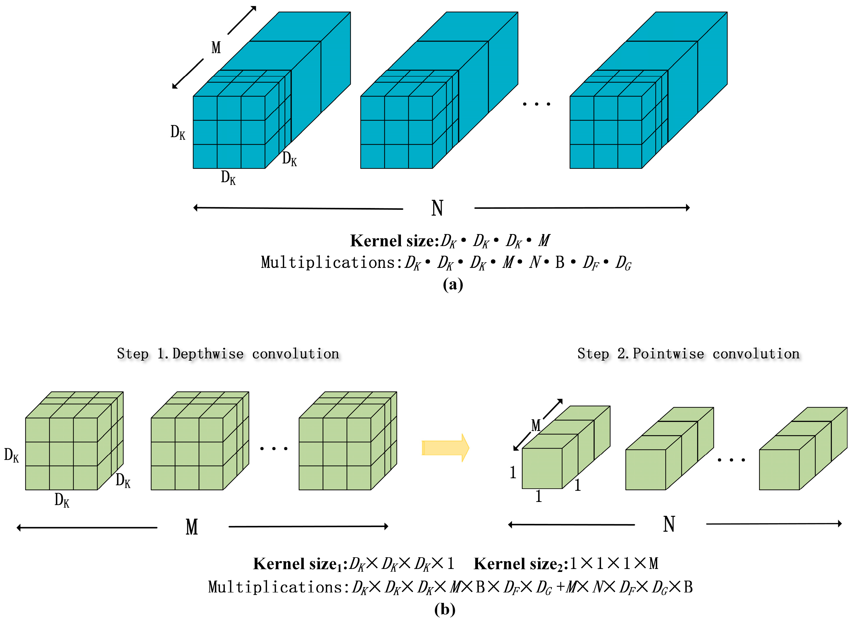
In most scenarios, both N and D_k typically exceed 2, leading to the ratio calculated previously being less than unity. This underscores that the computational requirements for depthwise separable convolution are substantially lower than for traditional 2D convolution. For instance, if we consider a 3 × 3 convolution kernel with 256 output channels, the computational workload for depthwise separable convolution would be approximately just 10% that of the conventional 2D convolution. This significant reduction in computational demands not only makes the network more efficient, but also expedites its training process. In Figure 3, panels (a) and (b) visually delineate the differences in convolutional kernel size and computational intricacy between standard 2D convolution and its depthwise separable counterpart.

When working with hyperspectral images, which are inherently three-dimensional data, employing the aforementioned 2D depthwise separable convolution falls short as it neglects inter-band relationships within each pixel. This compromises the comprehensive extraction of spectral characteristics. To address this shortcoming and tailor the approach to the idiosyncrasies of hyperspectral imagery, we introduce the concept of 3D depthwise separable convolution, which integrates 3D depthwise and 3D pointwise convolutions.

For a conventional 3D convolution layer, let us denote the kernel size by D_k and assume the parameters are organized as D_k × D_k × D_k × M × N, where M stands for the input feature map’s channel count and N is indicative of the output channels. To ensure seamless edge transitions, we implement appropriate padding. Thus, the input feature map dimensions are posited as M × D_F × D_G × B, where D_F and D_G define the height and width of the input data, and B specifies the band count. Consequently, we introduce the term Cost_3D-A to signify the computational complexity intrinsic to standard 3D convolution operations. The calculation of Cost_3D-A is delineated as follows:

$${\mathrm{Cost}}_{3\mathrm{D}-\mathrm{A}}={\mathrm{D}}_{\mathrm{K}}·{\mathrm{D}}_{\mathrm{K}}·{\mathrm{D}}_{\mathrm{K}}·\mathrm{M}·\mathrm{N}·\mathrm{B}·{\mathrm{D}}_{\mathrm{F}}·{\mathrm{D}}_{\mathrm{G}}$$

(4)

In the framework of 3D depthwise separable convolutions, the overall computational expense can be encapsulated by the term Cost_3D-DW. Within this construct, Cost_3D-D refers to the computational requirements for carrying out the depthwise convolution, while Cost_3D-P signifies the computational load associated with the pointwise convolution. The computational burden of Cost_3D-DW can be systematically quantified as follows:

$$\begin{array}{cc}\hfill {\mathrm{Cost}}_{3\mathrm{D}-\mathrm{D}\mathrm{W}}& ={\mathrm{Cost}}_{3\mathrm{D}-\mathrm{D}}+{\mathrm{Cost}}_{3\mathrm{D}-\mathrm{P}},\hfill \\ & ={\mathrm{D}}_{\mathrm{K}}·{\mathrm{D}}_{\mathrm{K}}·{\mathrm{D}}_{\mathrm{K}}·\mathrm{M}·\mathrm{B}·{\mathrm{D}}_{\mathrm{F}}·{\mathrm{D}}_{\mathrm{G}}+\mathrm{M}·\mathrm{N}·{\mathrm{D}}_{\mathrm{F}}·{\mathrm{D}}_{\mathrm{G}}·\mathrm{B}\hfill \end{array}$$

(5)

To evaluate the computational efficiency of 3D depthwise separable convolutions relative to their standard 3D convolution counterparts, one can compute the computational ratio as delineated below:

$$\begin{array}{cc}\hfill \frac{{\mathrm{Cost}}_{3\mathrm{D}-\mathrm{D}\mathrm{W}}}{{\mathrm{Cost}}_{3\mathrm{D}-\mathrm{A}}}& =\frac{{\mathrm{D}}_{\mathrm{K}}·{\mathrm{D}}_{\mathrm{K}}·{\mathrm{D}}_{\mathrm{K}}·\mathrm{M}·{\mathrm{B}·\mathrm{D}}_{\mathrm{F}}·{\mathrm{D}}_{\mathrm{G}}+\mathrm{M}·\mathrm{N}·{\mathrm{D}}_{\mathrm{F}}·{\mathrm{D}}_{\mathrm{G}}·\mathrm{B}}{{\mathrm{D}}_{\mathrm{K}}·{\mathrm{D}}_{\mathrm{K}}·{\mathrm{D}}_{\mathrm{K}}·\mathrm{M}·\mathrm{N}·\mathrm{B}·{\mathrm{D}}_{\mathrm{F}}·{\mathrm{D}}_{\mathrm{G}}},\hfill \\ & =\frac{1}{\mathrm{N}}+\frac{1}{{{\mathrm{D}}_{\mathrm{K}}}^3}.\hfill \end{array}$$

(6)

In most scenarios, both the convolution kernel size D_k and the number of output channels N are greater than 2. Consequently, the computational ratio derived from the above formula usually falls below 1, signifying a substantial reduction in computational load when employing 3D depthwise separable convolutions. Particularly, when D_k equals 3 and N is large, the computational overhead for 3D depthwise separable convolution can be diminished by approximately a factor of 27 compared to the standard 3D convolution. Figure 4 parts (a) and (b) graphically delineate disparities in convolutional kernel dimensions as well as computational complexities between the two convolutional techniques. Initially, for the 3D depthwise convolution represented in Figure 4b, Step 1, each channel is convolved with its own D_k × D_k × D_k × 1 independent convolution kernel. The corresponding computational demand for this 3D depthwise convolution stage is D_k × D_k × D_k × M × B × D_F × D_G. Subsequently, the output generated in Step 1 serves as the input for Step 2, which applies 3D pointwise convolution using a 1 × 1 × 1 × M kernel, yielding an output 3D tensor of dimensions N × D_F × D_G. In this computational phase, the incurred expense is defined as M × N × D_F × D_G × B. To sum it up, employing 3D depthwise separable convolutions comes with the advantages of parameter efficiency and diminished computational overhead, especially when contrasted with traditional 3D convolutional approaches.

2.2.2. Multiscale 3D Depthwise Separable Convolutional Network

Capitalizing on the merits of 3D depthwise separable convolution, we engineer a multiscale 3D depthwise separable convolutional architecture aimed at capturing a richer spectrum of spatial–spectral features. This network framework is comprised of dual multiscale 3D convolutional modules. Within each module, three parallel branches coexist, each employing convolution kernels of varying dimensions and counts. In the first branch, 1 × 1 × 1 standard 3D convolution is utilized for feature abstraction from the input dataset, with the kernel count being 16 and 32 in the initial and subsequent modules, respectively. The second branch incorporates both a 1 × 1 × 1 standard 3D convolution and a 3 × 3 × 3 depthwise separable 3D convolution for more elaborate feature extraction. Here, the number of kernels in the initial and secondary modules are designated as 8 and 16, and 16 and 32, respectively. As for the third branch, it leverages 1 × 1 × 1 standard 3D convolution along with 5 × 5 × 5 depthwise separable 3D convolution; the kernel counts here are set at 8 and 16 for the first module and 32 and 64 for the second. Interposed between the two convolution modules is a maximum pooling layer to facilitate spatial downsampling. Ultimately, the outputs from these branch-wise operations are concatenated and fed into the succeeding network layer. The implementation of 1 × 1 × 1 convolutional kernels serves to curtail the model’s weight parameters, thereby simplifying its complexity. Varied kernel sizes of 1 × 1 × 1, 3 × 3 × 3, and 5 × 5 × 5 allow the network to harvest features over multiple receptive field ranges [34]. To bolster the network’s non-linear expressive capabilities, we have integrated Batch Normalization (BN) layers and ReLU activation functions into each convolutional layer. Further, in our depthwise separable convolutions, we have fixed the stride to 1 and padding parameters to zero, enabling channel augmentation without altering the spatial dimensions, thus retaining detailed features. The network architecture is visually represented in Figure 5.

2.3. Two-Dimensional Convolution Module

2.3.1. Mixed-Domain Attention Mechanism CBAM

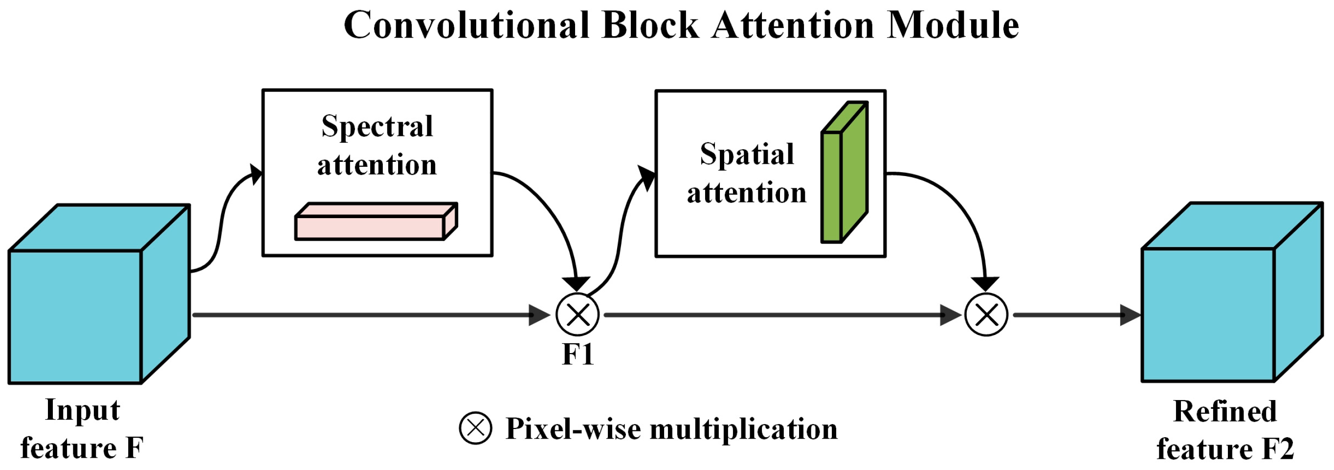
To emphasize pertinent spatial and spectral details while filtering out extraneous information, we integrate a CBAM into the 2D convolutional segment of our model [35]. This serves as a mixed-domain attention mechanism specializing in both spectral and spatial domains, as visualized in Figure 6. The CBAM system is bifurcated into a spectral attention segment and a spatial attention segment. Initially, the spectral attention module fine-tunes the input feature map, denoted as F, to generate a corrected version, F1. Subsequently, this intermediate feature map, F1, is further refined by the spatial attention mechanism to produce the ultimate feature map, F2.

The workings of the spectral attention module are detailed in Figure 7. The process initiates with the input feature map, denoted as F, being subject to both global max pooling and global average pooling. This step captures different semantic nuances within the data. Following this, a shared multi-layer perceptron extracts channel-specific feature attributes. A summation operation is then employed to amalgamate the two separate vectors derived from these pooling techniques, thereby generating a unified spectral attention feature vector. This integrated feature vector undergoes further refinement via the application of a Sigmoid activation function. The resultant output is the definitive spectral attention vector, formulated as per the equation given below:

$${\mathrm{M}}_{\mathrm{C}}\left(\mathrm{F}\right)=\mathsf{\sigma }\left(\mathrm{MLP}\left(\mathrm{AvgPool}\left(\mathrm{F}\right)\right)+\mathrm{MLP}\left(\mathrm{MaxPool}\left(\mathrm{F}\right)\right)\right).$$

(7)

In this framework, the input feature map is symbolized as F, and σ designates the Sigmoid activation function. The neural network layer that is shared across the channels is denoted as MLP. The terms AvgPool(F) and MaxPool(F) correspond to the actions of global average pooling and global max pooling executed on F, respectively. The ultimate spectral attention vector derived from this mechanism is represented by M_C(F). Subsequent to the application of the spectral attention scheme, a specific weight is allocated to each spectral channel. By element-wise multiplication of the synthesized spectral attention vector M_C with F, a new feature map F1 is procured.

As illustrated in Figure 8, the spatial attention mechanism functions by initially implementing global max and average pooling across the channel scope of the existing feature map, denoted as F1. This produces semantic indicators that, while distinct, are complementary to each other. After concatenation, they are processed through a convolutional stratum employing a kernel size of 7 × 7, succeeded by the application of a Sigmoid activation layer. The procedure culminates in the extraction of the spatial attention vector, as expressed in the subsequent mathematical formulation.

$${\mathrm{M}}_{\mathrm{s}}\left(\mathrm{F}1\right)=\mathsf{\sigma }\left({\mathrm{ƒ}}^{7\times 7}\right([\mathrm{AvgPool}\left(\mathrm{F}1\right);\mathrm{MaxPool}(\mathrm{F}1\left)\right]\left)\right)$$

(8)

In the formula associated with the spatial attention mechanism, F1 denotes the incoming feature map, while σ symbolizes the activation via the Sigmoid function. Moreover, ƒ^7×7 signifies a convolutional transformation with a 7 × 7 kernel. The operations AvgPool(F1) and MaxPool(F1) encapsulate the global average and max pooling over the channel dimension of F1, respectively. Ultimately, M_S(F1) is computed as the finalized spatial attention vector.

Following the employment of the spatial attention mechanism, the spatial attention vector M_S is element-wise multiplied with F1 to derive the conclusive feature map, F2.

2.3.2. CBAM Residual Dilated Convolutional Network

To enhance the model’s receptive capabilities, quicken its convergence, and refine its focus on particular local features, we devised a novel architecture by merging the CBAM attention mechanism with dilated convolutions within a residual framework. This architecture, dubbed “CBAM Residual Dilated Convolutional Network,” encompasses a primary module that boasts two dilated convolutions paired with dual CBAM attention units. Concurrently, an auxiliary module integrates one dilated convolution with a CBAM attention unit. These modules are interlinked via a unique residual bridge, facilitating advanced feature extraction. The comprehensive layout is depicted in Figure 9.

To implement 2D convolution on the feature map derived from the 3D convolution process, the number of bands, represented by b, is multiplied by the channel count, denoted by n. This operation transforms the b × m × m feature segment, which retains n original channels, into an m × m two-dimensional feature map, which is then channeled into the 2D convolution module. Owing to the expansive channel count resulting from the reshaping, an initial 3 × 3 2D convolution compresses the channels down to 64. Subsequently, through the interplay of the primary and auxiliary networks, individual elements are aggregated and activated, producing the final feature output. In the CBAM residual dilated convolution framework, each of the three dilated convolutions employs 64 3 × 3 kernels, a dilation rate set at 2, a stride of 1, and no padding. Additionally, every convolutional layer is enhanced with a BN layer and RELU activation to optimize the model’s data alignment.

3. Experimental Results and Discussion

3.1. Datasets

To assess the effectiveness of the HSIC approach introduced in this study, three well-known datasets, namely Indian Pines, Pavia University, and Salinas, have been selected.

The dataset from Indian Pines, captured by the AVIRIS sensor over a pine-laden region in Indiana, USA, originally comprised 220 wave bands. However, 20 of these bands, not reflected by water, were excluded. Consequently, 200 bands were retained for the final analysis. This dataset has a spatial dimension of 145 × 145 pixels, resulting in a total of 21,025 pixels. Out of these, 10,776 pixels, which serve as the background, are disregarded in the classification, while the composition of the 10,249 terrestrial pixel samples is detailed in

Table 1. Indian Pines dataset categories.

Category	Class Name	Color	Sample
1	Alfalfa		46
2	Corn-notill		1428
3	Corn-mintill		830
4	Corn		237
5	Grass-pasture		483
6	Grass-trees		730
7	Grass-pasture-mowed		28
8	Hay-windrowed		478
9	Oats		20
10	Soybean-notill		972
11	Soybean-mintill		2455
12	Soybean-clean		593
13	Wheat		205
14	Woods		1265
15	Buildings-Grass-Trees-Drivers		386
16	Stone-Steel-Towers		93

. Refer to Figure 10a,b for its false color image and authentic labels, respectively.

Pavia University’s dataset captured hyperspectral imagery from the University of Pavia, located in Northern Italy, using the ROSIS instrument. Boasting 610 × 340 pixels, it encompasses 42,776 terrestrial object pixels in

Table 2. Pavia University dataset categories.

Category	Class Name	Color	Sample
1	Asphalt		6631
2	Meadows		18649
3	Gravel		2099
4	Trees		3064
5	Painted metal sheets		1345
6	Bare soil		5029
7	Bitumen		1330
8	Self-blocking bricks		3682
9	Shadows		947

Initially comprising 115 bands, 12 were omitted due to noise interference, leaving 103 for the concluding analysis. The dataset spans nine categories, and its false color representation alongside actual labels can be viewed in Figure 10c,d.

Lastly, the Salinas dataset, sourced from the AVIRIS sensor over California’s Salinas Valley, exhibits a pixel size of 512 × 217 and boasts a spatial resolution pegged at 3.7m. Hosting 54,129 samples, this dataset features 16 distinct ground attributes, as described in

Table 3. Salinas dataset categories.

Category	Class Name	Color	Sample
1	Broccoli-green-weeds_1		2009
2	Broccoli-green-weeds_2		3726
3	Fallow		1976
4	Fallow-rough-plow		1394
5	Fallow-smooth		2678
6	Stubble		3959
7	Celery		3579
8	Grapes-untrained		11,271
9	Soil-vineyard-develop		6203
10	Corn-senesced-green-weeds		3278
11	Lettuce-romaine-4wk		1068
12	Lettuce-romaine-5wk		1927
13	Lettuce-romaine-6wk		916
14	Lettuce-romaine-7wk		1070
15	Vineyard-untrained		7268
16	Vineyard-vertical-trellis		1807

. Post-adjustment, the concluding analysis employs 204 bands. Figure 10e,f present the false color rendition and genuine labels of this dataset.

3.2. Model Setting and Experimental Parameters

In our research, we subjected the HSIC technique to rigorous testing on the datasets previously discussed. All these comparative analyses were carried out on a laptop, powered by a 12th Gen Intel(R) Core(TM) i9-12900H processor, fortified with 16.0 GB of RAM, and complemented by an NVIDIA GeForce RTX 3060 Laptop GPU. The computational environment leaned on the Windows 11 OS and the deep learning infrastructures of Pytorch1.10.2 paired with CUDA11.3.

Given that hyperparameters can influence the categorization capability of the algorithm, we strategically selected hyperparameters with the most pronounced impact. The Adam optimizer was used for model optimization in this study and the learning rate was set as 0.5, 0.1, 0.05, 0.01, 0.005, 0.001, 0.0005, and 0.0001. Through continuous testing and adjustment, it was found that the MDRDNet performed best among the three hyperspectral datasets when the learning rate was set as 0.001. With the cross-entropy function designated as our loss function, we allocated 10% of our data for training purposes, leaving the remaining 90% for evaluation. The model’s efficacy was ascertained using three key metrics: overall accuracy (OA), average accuracy (AA), and the Kappa coefficient. High values across these parameters typically signify optimal model classification. Figure 11 shows the change curves of the loss value and accuracy of the MDRDNet which was trained and tested on the IP, PU, and SA datasets, respectively. From Figure 11, as the epoch increased, the loss value continued to decrease and the accuracy increased. After a number of trainings, the loss value and accuracy of the MDRDNet on the IP, PU, and SA datasets tended to be stable, and the model reached convergence when epochs were greater than 50, 20, and 20, respectively. In order to unify the hyperparameters of the model, the epoch was set to 100.We have also planned further analyses to determine the best values for batch size, channel numbers, spatial input dimensions, and dropout rates.

3.2.1. Batchsize

Batchsize represents the number of patched-images for each training of our model. A larger batchsize can improve the memory utilization and parallelization efficiency of large matrix multiplications, enhance model convergence, and reduce the running time of each epoch. However, if the batchsize is too large, it will occupy a large memory capacity and lead to local optimality. In our research, we analyzed batchsizes of 32, 64, 128, 256, and 512 across the three datasets, with results showcased in Figure 12.

The illustrated data reveal that for the PU dataset, the batchsize of 64 yielded the best results across OA, AA, and Kappa metrics. Conversely, for both the IP and SA datasets, the batchsize of 128 proved optimal.

The process of the dimensionality reduction of hyperspectral data via PCA demands the careful selection of the channel number. Overshooting this number could lead to redundant information, whereas an unduly low number might compromise accuracy. In our research, we analyzed the channel numbers 15, 20, 25, 30, and 35 across the three datasets, with results showcased in Figure 13.

The illustrated data reveal that for the IP dataset, a channel number of 25 yielded the best results across OA, AA, and Kappa metrics. Conversely, for both the UP and SA datasets, a channel number of 20 proved optimal.

3.2.2. Spatial Input Sizes

In this study, by employing neighborhood extraction, we regarded all surrounding pixels within a certain region as a collective sample block. The size of this sample block is crucial: an excessively large block would encompass too many pixels, potentially reducing the precision of classification. On the other hand, a diminutive block might lack the spatial attributes necessary to accurately determine the class of the central pixel. To discern the ideal spatial input dimensions, we analyzed a series of sizes: 15 × 15, 17 × 17, 19 × 19, 21 × 21, 23 × 23, and 25 × 25, using three public datasets as benchmarks. As illustrated in Figure 14, a spatial dimension of 21 × 21 consistently yielded superior results, as evidenced by the OA, AA, and Kappa metrics across the referenced datasets.

3.2.3. Dropout

The dropout technique permits neurons to be intermittently excluded from the network based on a pre-defined probability. This not only serves as an effective countermeasure against over-fitting, but also augments the operational speed of the model [36]. In this study, several dropout values were tested—specifically 0.2, 0.3, 0.4, 0.5, and 0.6—across three benchmark datasets to determine the most optimal setting. Referencing Figure 15, a dropout value of 0.5 manifested the most commendable classification outcomes in terms of OA, AA, and Kappa for the IP and UP datasets. Conversely, for the SA dataset, a dropout value of 0.4 was observed to yield the most favorable results.

It is vital for examining the stability of the model to carry out the sensitivity analysis of hyperparameters in deep learning. Optimal hyperparameters can maximize the performance of the model [37,38]. Different hyperparameters will have different effects on the OA, AA, and Kappa of the MDRDNet. The optimal hyperparameter settings for IP, PU, and SA datasets are shown in

Table 4. Optimal hyperparameter settings for different datasets.

Datasets	Learning Rate	Epochs	Batchsize	Channel Number	Spatial Input Sizes	Dropout
IP	0.0001	100	128	25	21 × 21	0.5
PU	0.0001	100	64	20	21 × 21	0.5
SA	0.0001	100	128	20	21 × 21	0.4

. As an adjustable parameter on the loss function, the learning rate directly controls the magnitude of network gradient updates during training and affects the effective tolerance of the model. In addition, epochs controls the step size of MDRDNet gradient descent, and batchsize determines the direction of MDRDNet gradient descent. Meanwhile, the performance of the model will be affected by the epochs and batchsize. The channel number and spatial input sizes are hyperparameters affected by remote sensing data sources. The MDRDNet can be trained scientifically after exploring the optimal values of the channel number and spatial input sizes to improve resource utilization. Dropout, as a regularization parameter, usually prevents overfitting between fully connected layers and makes the model more generalizable. In summary, the sensitivity of MDRDNet hyperparameters from high to low is learning rate, epochs, batchsize, channel number, spatial input sizes, and dropout.

3.3. Comparative Experiment

In this study, three public hyperspectral datasets are utilized for a comparative assessment. For each of these datasets, we allocate 10% for training, with the remaining portion designated for testing purposes. To evaluate the models, we considered metrics such as the overall accuracy (OA), average accuracy (AA), and the Kappa coefficient. Our proposed MDRDNet is meticulously contrasted against six alternative methodologies, encompassing traditional approaches such as SVM, contemporary methods such as 2D-CNN and 3D-CNN, the HybridSN [20] employing hybrid convolution, SSRN [19] leveraging the spectral–spatial residual, and the innovative LRCNet [33].

Table 5. The classification accuracy comparison for the IP dataset (%).

Classes	SVM	2D-CNN	3D-CNN	SSRN	HybridSN	LRCNet	MDRDNet
Alfalfa	92.73	93.02	100	97.62	100	95.12	97.62
Corn-notill	80.42	85.16	98.62	96.32	98.94	98.87	99.84
Corn-mintill	91.11	94.03	89.06	99.05	97.64	98.54	99.73
Corn	88.39	93.14	100	97.94	97.67	100	100
Grass-pasture	74.35	92.68	98.21	100	98.62	99.54	97.3
Grass-trees	92.44	93.73	97.09	99.69	97.47	99.69	99.54
Grass-pasture-mowed	100	100	100	100	100	100	100
Hay-windrowed	95.08	100	99.77	100	98.17	97.51	99.77
Oats	78.95	72.22	100	90	85.71	94.74	100
Soybean-notill	93.86	96.96	96.8	98.62	96.23	98.85	98.29
Soybean-mintill	85.91	97.02	96.9	96.93	97.9	97.69	98.12
Soybean-clean	58.16	93.71	97.25	97.67	99.6	98.86	98.68
Wheat	98.78	99.49	97.93	100	100	100	98.38
Woods	81.39	96.24	100	99.82	98.52	99.39	99.56
Buildings-Grass-Trees-Drivers	91.98	94.38	100	99.41	98.83	99.14	98.29
Stone-Steel-Towers	85.01	98.65	98.61	93.42	89.36	93.02	96.39
OA(%)	84.09	94.21	97.25	98.2	98.04	98.62	98.83
AA(%)	85.53	93.78	98.14	97.91	98.01	98.19	98.62
K × 100	82.24	93.45	96.88	97.95	97.88	98.43	98.84

,

Table 6. The classification accuracy comparison for the UP dataset (%).

Classes	SVM	2D-CNN	3D-CNN	SSRN	HybridSN	LRCNet	MDRDNet
Asphalt	88.57	97.99	99.49	99.15	99.15	100	100
Meadows	96.81	99.66	99.98	99.88	99.93	99.95	99.96
Gravel	87.22	93.27	99.15	97.45	98.89	100	99.1
Trees	96.64	98.94	99.97	99.79	99.82	98.28	99.06
Painted metal sheets	99.92	99.92	100	100	100	100	100
Bare soil	98.36	99.51	99.86	99.98	99.98	100	99.98
Bitumen	94.35	96.62	95.94	99.29	99.16	98.92	99.92
Self-blocking bricks	84.1	94.54	93.15	98.64	98.95	99.58	99.37
Shadows	76.29	93.96	97.57	98.22	98.04	98.56	100
OA(%)	93.7	98.37	99.04	99.49	99.61	99.75	99.81
AA(%)	91.36	97.16	98.35	99.15	99.32	99.61	99.71
K × 100	91.77	97.85	98.73	99.32	99.48	99.67	99.75

and

Table 7. The classification accuracy comparison for the SA dataset (%).

Classes	SVM	2D-CNN	3D-CNN	SSRN	HybridSN	LRCNet	MDRDNet
Broccoli-green-weeds_1	99.64	100	99.85	99.6	100	100	100
Broccoli-green-weeds_2	96.72	99.68	100	100	100	100	100
Fallow	92.78	99.39	96.93	99.9	100	100	100
Fallow-rough-plow	94.12	96.99	97.04	98.91	99.45	99.76	100
Fallow-smooth	96.24	100	99.76	100	100	99.96	100
Stubble	100	99.97	99.85	99.97	99.92	99.94	99.89
Celery	100	100	99.49	100	99.78	100	100
Grapes-untrained	93.72	97.79	97.62	99.28	99.99	100	100
Soil-vineyard-develop	99.98	100	99.47	99.98	100	100	100
Corn-senesced-green-weeds	99.54	89.79	99.26	99.72	99.49	100	100
Lettuce-romaine-4wk	98.49	100	100	99.81	99.38	100	100
Lettuce-romaine-5wk	100	100	99.69	100	100	100	100
Lettuce-romaine-6wk	97.44	98.25	99.34	99.12	100	100	100
Lettuce-romaine-7wk	96.89	97.02	99.15	100	100	100	100
Vineyard-untrained	87.69	97.13	98.49	98.71	100	100	100
Vineyard-vertical-trellis	98.55	100	100	99.89	100	100	100
OA(%)	95.95	98.26	98.9	99.59	99.92	99.98	99.99
AA(%)	95.99	98.5	99.12	99.68	99.88	99.98	99.99
K × 100	95.48	98.06	98.78	99.54	99.89	99.97	99.99

catalog the OA, AA, and Kappa metrics derived from different techniques based on the three public datasets.

3.3.1. Experimental Results of IP

On reviewing the IP dataset sample counts in Table 1, a considerable disparity in pixel counts across different terrestrial object categories is evident. For instance, categories such as Grass-pasture-mowed (seventh) and Oats (ninth) register a mere 28 and 20 pixels, respectively. In contrast, the Soybean-mintill category (eleventh) boasts 2455 pixels, thus pointing to a stark imbalance in training sample sizes. This variability in sample size offers an opportunity to robustly assess the model’s classification capabilities under constrained sample conditions.

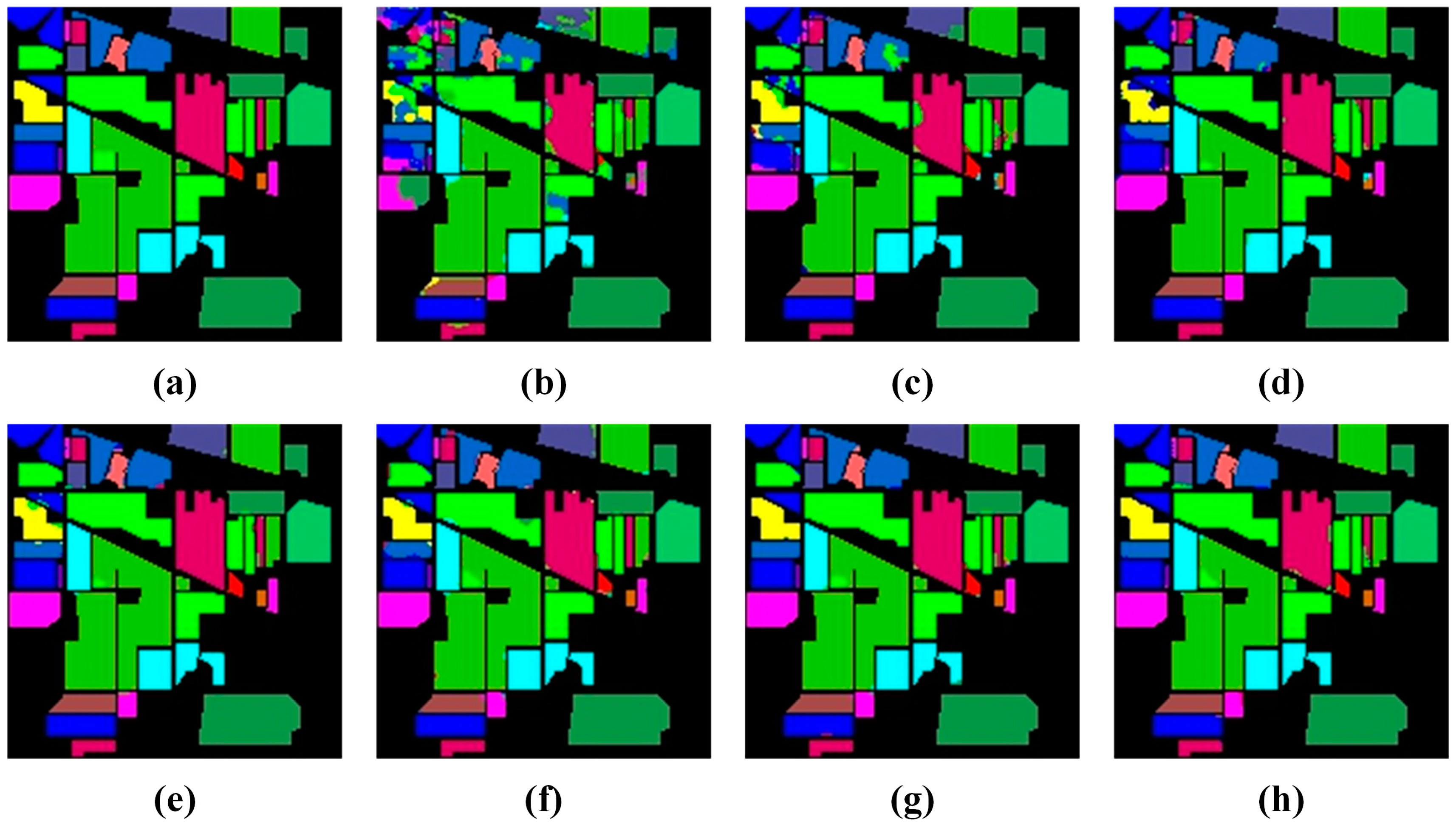
Table 5 details the performance of seven diverse algorithms applied to the IP dataset. Notably, the MDRDNet introduced in this study outperforms the others, registering OA, AA, and Kappa scores of 98.83%, 98.62%, and 98.84%, respectively. The OA of the MDRDNet surpasses its closest competitor by 0.21%, and its AA exceeds the second-best by 0.43%. This considerable enhancement in classification performance underscores the MDRDNet’s prowess, especially when grappling with imbalanced training datasets. The classification landscapes for the IP dataset are illustrated in Figure 16.

The training samples of the IP dataset were divided into 5%, 10%, 20%, and 30% to test the classification performance. The OA, AA, and Kappa coefficients are shown in

Table 8. The classification accuracies obtained using a small number of training samples (%).

Proportion of Training Samples	OA	AA	Kappa
30%	99.57	99.08	99.51
20%	99.22	98.99	99.11
10%	98.83	98.62	98.84
5%	96.77	96.89	96.33

. As the proportion of training samples increases, OA, AA, and Kappa all improve to varying degrees. When the training sample ratio is 30%, OA, AA, and Kappa can reach 99.57%, 99.08%, and 99.51%. However, when the training sample ratio is 5%, OA, AA, and Kappa decrease to 96.77%, 96.89%, and 96.33%.

3.3.2. Experimental Results of UP

Table 6 offers a comparative assessment of seven varied methodologies’ performances on the UP dataset. From this analysis, it is apparent that our MDRDNet continues to maintain its superiority on the UP dataset, registering optimal scores in the OA, AA, and Kappa coefficients. Specifically, the OA achieved an impressive 99.81%, edging out its nearest competitor by a margin of 0.06%. Similarly, AA clocked in at 99.71%, surpassing the runner-up by 0.1%.

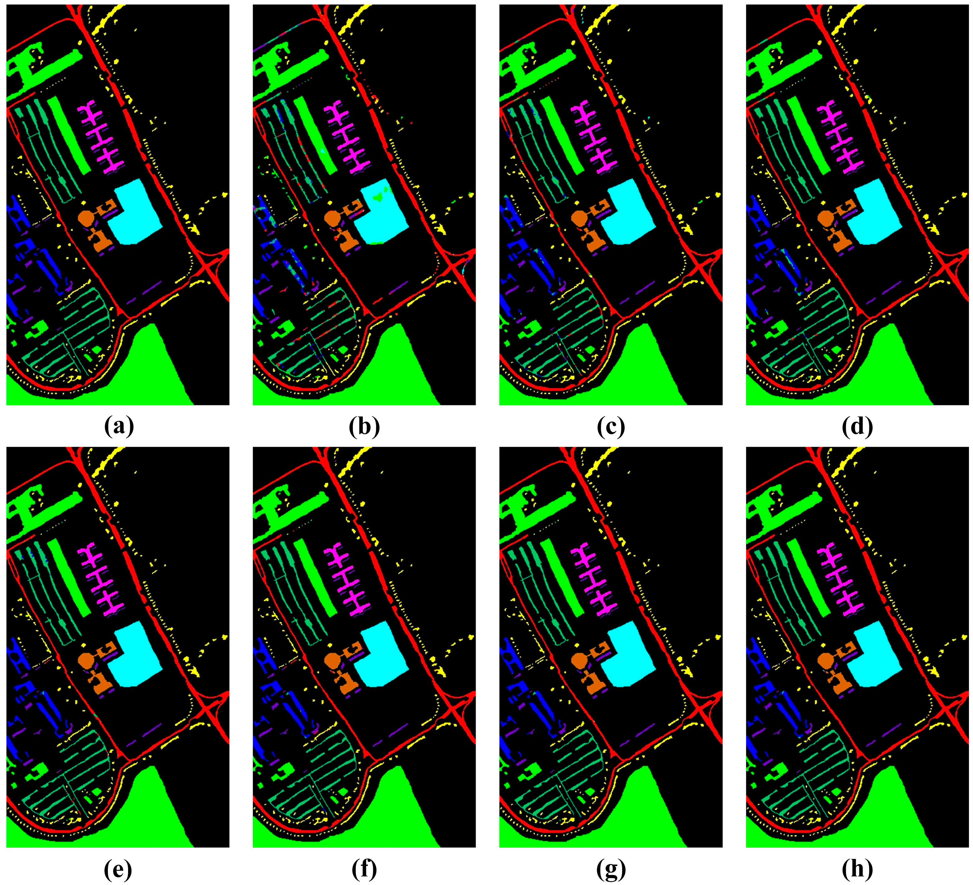
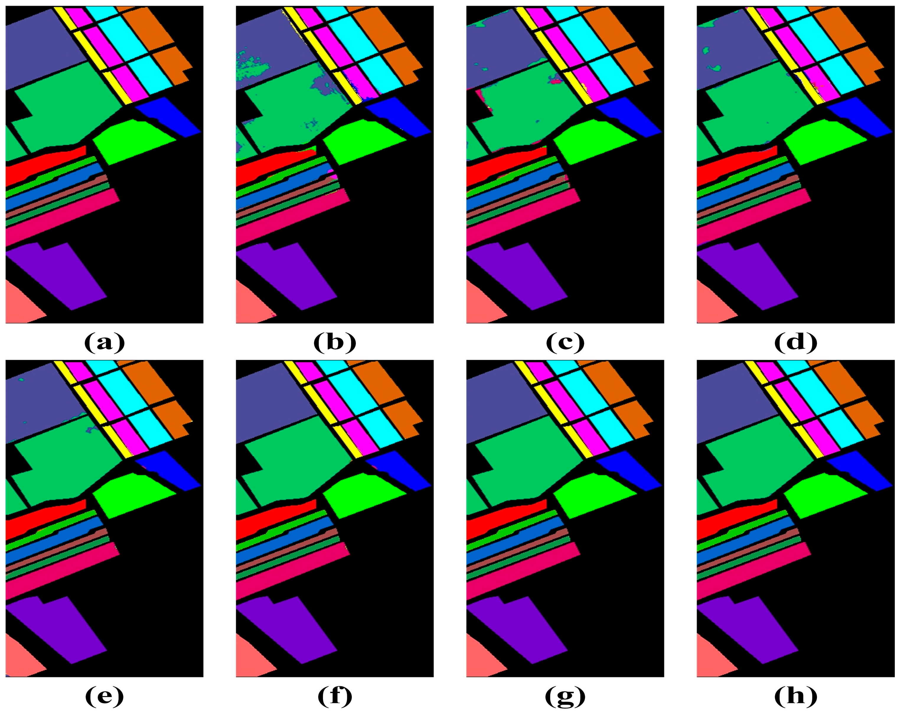
Figure 17 delineates the classification outcomes for the UP dataset. A cursory glance reveals that the conventional SVM approach is marred by significant speckle noise, rendering its OA and AA at a mere 93.7% and 91.77%, respectively. The limitation of SVM, primarily its inability to holistically harness both spatial and spectral features for improved image categorization, underscores this performance. Although deep learning-driven classification techniques harness spatial–spectral characteristics, leading to markedly enhanced classification results, certain techniques such as 3D-CNN, SSRN, and HybridSN are still not devoid of misclassification instances. In stark contrast, LRCNet, by leveraging depthwise separable convolution and receptive field strategies, minimizes misclassification occurrences. Consequently, the MDRDNet, as introduced in this study, provides classification results that mirror true categories, underscoring its evident superior classification efficacy.

3.3.3. Experimental Results of SA

Table 7 outlines the performance metrics of seven distinct methodologies on the SA dataset. Notably, the SA dataset has a considerable number of training samples across its categories, which in comparison to the IP and UP datasets, translates to a markedly higher classification accuracy. The data presented illustrate the prowess of the MDRDNet, as discussed in this study. Remarkably, the MDRDNet achieves a flawless classification rate of 100% across 15 sample types within the SA dataset. Furthermore, for the sixth category, labeled ‘Stubble’, it boasts a near-perfect accuracy of 99.89%. With an impressive tally of 99.99% across the OA, AA, and Kappa metrics, the MDRDNet distinctly stands out, demonstrating a classification output that closely mirrors actual object maps. To further visualize this, Figure 18 delineates the classification results for the SA dataset.

3.4. Ablation Experiment

To ascertain the role of multiscale 3D depthwise separable convolutions in influencing classification precision, ablation studies focusing on 3D convolutional components were conducted. This paper’s MDRDNet is juxtaposed against two enhanced network prototypes, dubbed Net1 and Net2, both pivoting around 3D convolutional elements. Specifically, Net1 substitutes the 3D depthwise separable convolution within the 3D convolutional block with a conventional 3D convolution, retaining other architectural facets. Meanwhile, Net2 transitions the 3D depthwise separable convolution within the 3D convolutional segment to the three-tier 3D standard convolution observed in HybridSN, again, without other structural alterations. The comparative analyses were implemented under identical experimental conditions. Owing to the uneven distribution of training samples in the IP dataset, which serves as an optimal benchmark for model classification prowess, it was earmarked for this evaluative exercise.

Table 9. Results of 3D module ablation experiment (%).

Networks	OA	AA	Kappa	Params	Flops (MB)
MDRDNet	98.83	98.62	98.84	2,015,746	94.46
Net1	98.46	98.41	98.25	2,187,410	633.15
Net2	98.18	98.22	97.93	3,101,842	125.68
HybridSN	98.04	98.01	97.88	5,122,176	247.68
LRCNet	98.62	98.19	98.43	3,857,330	95.71

tabulates both classification outcomes and computational metrics such as Parameters (Params) and floating point operations (Flops). A scrutiny of the results reveals that Net1, in terms of OA, AA, and Kappa metrics, substantially outstrips Net2, simultaneously showcasing a reduced parameter count. This underlines the efficacy of the multiscale hybrid convolutional amalgamation in amplifying model classification acuity. A side-by-side assessment between the MDRDNet and Net1 underscores that transitioning from a standard 3D convolution to a 3D depthwise separable convolution not only trims the model’s parameter and computational overhead, but also augments its classification precision, attesting to the potency of the depthwise separable convolution within the 3D realm. From Table 7, the Params and Flops of the MDRDNet were 2015746 and 94.46MB, respectively. Meanwhile, the Params and Flops of the HybridSN and LRCNet were 5122176, 247.68MB, 3857330, and 95.71MB, respectively. Obviously, the Params and Flops of the MDRDNet were less than those of HybridSN and LRCNet.

To evaluate the influence of both the CBAM attention mechanism and dilated convolution within the context of the residual framework on classification precision, an ablation study targeting the 2D convolutional segment was undertaken. The MDRDNet, as presented in this research, was benchmarked against two refined network architectures, named Net3 and Net4, each based on the 2D convolutional paradigm. Within Net3, the trio of 2D dilated convolutions present in the 2D convolutional division was substituted with a trio of conventional 2D convolutions, with the rest of the design being static. Conversely, Net4 saw the excision of the three CBAM attention schemas in its 2D convolutional section, with all other elements being preserved. Every comparative trial was set in an invariant experimental milieu, using the IP dataset as the subject of evaluation, with the resultant classifications illustrated in

Table 10. Results of 2D module ablation experiment (%).

Networks	OA	AA	Kappa
MDRDNet	98.83	98.62	98.84
Net3	98.35	98.18	98.12
Net4	98.26	97.85	98.03

. An analysis of the Net4 outcomes reveals that, when divested of the CBAM attention scheme in MDRDNet’s 2D convolution module, there is a pronounced dip in model classification fidelity. Specifically, the metrics of OA, AA, and Kappa exhibit reductions of 0.57%, 0.77%, and 0.81%, respectively, attesting to CBAM’s capability to bolster model precision by accentuating the assimilation of pivotal spatial and spectral data. When stacked against Net3, the MDRDNet’s OA, AA, and Kappa indices exceed by 0.48%, 0.44%, and 0.72%, respectively, indicating that a designated expansion of the receptive domain in 2D convolution enhances model classification prowess.

In order to determine the impact of the dilation rate on the model classification performance, three baseline models were designed, named Net5, Net6, and Net7, respectively. Meanwhile, the dilation rates of Net5, Net6, and Net7 were set to one, three and four, respectively, and compared with the dilation rate of two in the MDRDNet. From

Table 11. The classification accuracy of different receptive fields (%).

Networks	Dilation Rate	OA	AA	Kappa
MDRDNet	2	98.83	98.62	98.84
Net5	1	98.15	98.57	97.9
Net6	3	98.55	98.2	98.35
Net7	4	97.46	97.39	97.11

, where the dilation rate is one, the OA, AA, and Kappa of the model are 98.15%, 98.57%, and 97.9%, which are reduced by 0.68%, 0.05%, and 0.94%, respectively, compared with the MDRDNet. When the dilation rate increases, the classification accuracy of the model decreases to a certain extent. The OA, AA, and Kappa of Net6 were 98.55%, 98.2%, and 98.35%, while Net7’s OA, AA, and Kappa were only 97.46%, 97.39%, and 97.11%.

4. Discussion

4.1. Optimal Hyperparameters for HSIs

In order to determine the optimal hyperparameters of the model, the MDRDNet was trained on three public datasets. Hyperparameters such as learning rate, batchsize, number of channels, spatial input size, and dropout will all have a certain impact on the final classification result. The learning rate determines the convergence speed of the model backpropagation, and the size of the batchsize affects the memory utilization and parallelization efficiency of the model [39]. The size of the input network spectral dimension is affected by the channel number, and the size of spatial input sizes determines the amount of spatial information and redundant information [40]. The fitting degree and processing speed of the model are determined by the size of the dropout [41]. From Figure 12, Figure 13, Figure 14 and Figure 15, the optimal values of the hyperparameters for different hyperspectral datasets are different. Therefore, it is crucial for hyperspectral image classification experiments to determine the optimal hyperparameters because it determines whether the model can achieve optimal performance.

4.2. Optimal Model for HSIs

4.2.1. Classic Model

The classification results of comparative experiments are shown in Table 4, Table 5, Table 6 and Table 8 and Figure 16, Figure 17 and Figure 18. It is evident from the results that the MDRDNet proposed in this paper achieved the highest Overall Accuracy (OA), Average Accuracy (AA), and Kappa coefficients. In the IP, PU, and SA datasets, the OA reached 98.83%, 99.81%, and 99.99%, respectively. Compared with the traditional classification method SVM, the accuracy of the deep learning-based classification method was significantly improved. This is because deep learning models can automatically extract features and make full use of spectral joint features for classification [42]. In addition, the combination of 2D and 3D convolution can extract spatial and spectral information more comprehensively to extract more discriminative features. Compared with 2D-CNN and 3D-CNN methods, the model accuracy of SSRN [19], HybridSN [20], LRCNet [33], and the MDRDNet was greatly improved. Due to the incorporation of depth separable convolutions and receptive field strategies, the LRCNet exhibited a significant improvement in the OA, AA, and Kappa coefficients compared to SSRN and HybridSN. As shown in Table 7, the OA, AA, and Kappa of the MDRDNet were better than the LRCNet, and the number of parameters and Flops of the model were also reduced. Therefore, multi-scale fusion based on 3D depth-separable convolution and the residual module combining CABM and dilated convolution can boost feature extraction for ground object identification.

4.2.2. Baseline Model

The ablation experiments were conducted on the 3D convolution module and 2D convolution module of the MDRDNet in this study. Net1 substitutes the 3D depthwise separable convolution within the 3D convolutional block with a conventional 3D convolution. Net2 transitions the 3D depthwise separable convolution within the 3D convolutional segment to the three-tier 3D standard convolution observed in HybridSN. Based on Net1 and Net2, 3D depthwise separable convolution and multi-scale fusion strategies were introduced into the MDRDNet, respectively. As can be seen from Table 7, the multi-scale fusion strategy and deep separability technology not only improved the classification accuracy of the model, but also significantly reduced the Params and Flops of the model. Therefore, a new approach to solve the computational intensity issue in 3D convolutions was provided. Within Net3, the trio of 2D dilated convolutions present in the 2D convolutional division was substituted with a trio of conventional 2D convolutions. Moreover, Net4 saw the excision of the three CBAM attention schemas in its 2D convolutional section. Based on Net3 and Net4, receptive fields and CBAM attention mechanisms were introduced into MDRDNet, respectively. As can be seen from Table 9, by introducing dilated convolution and CBAM attention mechanism into the residual structure, the classification accuracy of the model has been effectively improved. In order to further explore the impact of different dilation rates in the 2D convolution module on the model classification results, the dilation rates of the three expansion convolutions were set to 1, 3, and 4, respectively, and named as Net5, Net6, and Net7. As shown in Table 10, when the expansion rate was two, the MDRDNet had the highest classification accuracy, which was better than Net5–Net7. Therefore, within an appropriate expansion rate range, when the attention mechanism of the dilated convolution and CBAM was introduced into the residual structure, the classification accuracy of the model was optimal.

4.3. Limitations and Prospects

In this study, the issues of insufficient spectral information extraction and high computational complexity in hyperspectral image classification were solved. However, in the case of small samples, it is crucial to learn most of the spatial and spectral features from a small number of training samples. Hyperspectral image classification is sensitive to imbalanced datasets in predicted classes. In future research, we will focus on solving the above problems.

5. Conclusions

In the current study, our main contribution is the introduction of the MDRDNet, which employs a blend of 2D and 3D hybrid convolution tailored for HSIC tasks. For the 3D convolutional segment, a unique approach has been adopted where 3D depthwise separable convolution technology is harmonized with a multiscale feature amalgamation approach. This combination not only curtails parameter volume, but also ensures that both spatial and spectral details are comprehensively harnessed. Turning our attention to the 2D convolutional segment, it boasts the integration of the CBAM attention schema and the dilation in convolution, embedded within the residual framework. This integration does not only expand the receptive scope, but also bolsters the feature recognition capabilities for terrestrial objects. To affirm the prowess of the MDRDNet as conceived in this study, evaluations were undertaken across three publicly accessible datasets. In juxtaposition to several contemporary classification paradigms, our MDRDNet exhibited superior competitiveness. The overall accuracy of the MDRDNet reached 98.83%, 99.81%, and 99.99% on the three datasets, respectively. Furthermore, dissecting experiments encompassing 2D and 3D convolutional components revealed that both the multiscale 3D depthwise separable convolution and the CBAM-augmented residual dilated convolution can significantly elevate the model’s classification accuracy. This reinforces the potential of this technique in HSIC applications. In the future, we will focus on solving the problems of small sample situations and imbalanced datasets in hyperspectral image classification.

References

1. Zhang, W.; Song, H.; He, X.; Huang, L.; Zhang, X.; Zheng, J.; Shen, W.; Hao, X.; Liu, X. Deeply learned broadband encoding stochastic hyperspectral imaging. Light Sci. Appl. 2021, 10, 108. [Google Scholar] [CrossRef] [PubMed]
2. Aneece, I.; Thenkabail, P.S. DESIS and PRISMA: A study of a new generation of spaceborne hyperspectral sensors in the study of world crops. In Proceedings of the 2021 IEEE International Geoscience and Remote Sensing Symposium IGARSS, Brussels, Belgium, 11–16 July 2021; p. 479. [Google Scholar]
3. Stuart, M.B.; Davies, M.; Hobbs, M.J.; Pering, T.D.; Mcgonigle, A.J.; Willmott, J.R. High-resolution hyperspectral imaging using low-cost components: Application within environmental monitoring scenarios. Sensors 2022, 22, 4652. [Google Scholar] [CrossRef] [PubMed]
4. Okada, N.; Maekawa, Y.; Owada, N.; Haga, K.; Shibayama, A.; Kawamura, Y. Automated identification of mineral types and grain size using hyperspectral imaging and deep learning for mineral processing. Minerals 2020, 10, 809. [Google Scholar] [CrossRef]
5. Fabelo, H.; Ortega, S.; Ravi, D.; Kiran, B.R.; Sosa, C.; Bulters, D.; Sarmiento, R. Spatio-spectral classification of hyperspectral images for brain cancer detection during surgical operations. PLoS ONE 2018, 13, e0193721. [Google Scholar] [CrossRef]
6. Hupel, T.; Stütz, P. Adopting Hyperspectral Anomaly Detection for Near Real-Time Camouflage Detection in Multispectral Imagery. Remote Sens. 2022, 14, 3755. [Google Scholar] [CrossRef]
7. Lv, W.; Wang, X. Overview of hyperspectral image classification. J. Sens. 2020, 2020, 4817234. [Google Scholar] [CrossRef]
8. Bigdeli, B.; Samadzadegan, F.; Reinartz, P. A multiple SVM system for classification of hyperspectral remote sensing data. J. Indian Soc. Remote 2013, 41, 763–776. [Google Scholar] [CrossRef]
9. Xia, J.; Falco, N.; Benediktsson, J.A.; Du, P.; Chanussot, J. Hyperspectral image classification with rotation random forest via KPCA. IEEE J. Sel. Top. Appl. Earth Obs. Remote Sens. 2017, 10, 1601–1609. [Google Scholar] [CrossRef]
10. Ou, X.; Zhang, Y.; Wang, H.; Tu, B.; Guo, L.; Zhang, G.; Xu, Z. Hyperspectral image target detection via weighted joint K-nearest neighbor and multitask learning sparse representation. IEEE Access 2019, 8, 11503–11511. [Google Scholar] [CrossRef]
11. Zou, S.; Chen, H.; Zhou, H.; Chen, J. An intelligent image feature recognition algorithm with hierarchical attribute constraints based on weak supervision and label correlation. IEEE Access 2020, 8, 105744–105753. [Google Scholar] [CrossRef]
12. Yang, Y.; Zhou, Y.; Chen, J.N. Hyperspectral image classification based on multi-scale hybrid convolutional network. Chin. J. Liq. Cryst. Disp. 2023, 38, 368–377. [Google Scholar] [CrossRef]
13. Audebert, N.; Le Saux, B.; Lefèvre, S. Deep learning for classification of hyperspectral data: A comparative review. IEEE Geosci. Remote Sens. Mag. 2019, 7, 159–173. [Google Scholar] [CrossRef]
14. Liu, B.; Yu, X.C.; Zhang, P.Q.; Tan, X. Deep 3D convolutional network combined with spatial-spectral features for hyperspectral image classification. Acta Geod. Cartogr. Sin. 2019, 48, 53–63. [Google Scholar]
15. Hu, W.; Huang, Y.; Wei, L.; Zhang, F.; Li, H. Deep convolutional neural networks for hyperspectral image classification. J. Sens. 2015, 2015, 258619. [Google Scholar] [CrossRef]
16. Cao, X.; Zhou, F.; Xu, L.; Meng, D.; Xu, Z.; Paisley, J. Hyperspectral image classification with Markov random fields and a convolutional neural network. IEEE Trans. Image Process. 2018, 27, 2354–2367. [Google Scholar] [CrossRef]
17. Zhao, W.; Du, S. Spectral–spatial feature extraction for hyperspectral image classification: A dimension reduction and deep learning approach. IEEE Trans. Geosci. Remote Sens. 2016, 54, 4544–4554. [Google Scholar] [CrossRef]
18. Shen, J.; Zheng, Z.; Sun, Y.; Zhao, M.; Chang, Y.; Shao, Y.; Zhang, Y. HAMNet: Hyperspectral image classification based on hybrid neural network with attention mechanism and multi-scale feature fusion. Int. J. Remote Sens. 2022, 43, 4233–4258. [Google Scholar] [CrossRef]
19. Zhang, X. Improved Three-Dimensional Inception Networks for Hyperspectral Remote Sensing Image Classification. IEEE Access 2023, 11, 32648–32658. [Google Scholar] [CrossRef]
20. Zhong, Z.; Li, J.; Luo, Z.; Chapman, M. Spectral-spatial residual network for hyperspectral image classification: A 3-D deep learning framework. IEEE Trans. Geosci. Remote Sens. 2017, 56, 847–858. [Google Scholar] [CrossRef]
21. Roy, S.K.; Krishna, G.; Dubey, S.R.; Chaudhuri, B.B. HybridSN: Exploring 3-D-2-D CNN feature hierarchy for hyperspectral image classification. IEEE Geosci. Remote Sens. Lett. 2019, 17, 277–281. [Google Scholar] [CrossRef]
22. Zhao, C.; Zhao, H.; Wang, G.; Chen, H. Hybrid depth-separable residual networks for hyperspectral image classification. Complexity 2020, 2020, 4608647. [Google Scholar] [CrossRef]
23. Howard, A.G.; Zhu, M.; Chen, B.; Kalenichenko, D.; Wang, W. Mobilenets: Efficient convolutional neural networks for mobile vision applications. arXiv 2017, arXiv:1704.04861. [Google Scholar]
24. Yan, W.; Qi, L. Fast 3D-CNN Combined with Depth Separable Convolution for Hyperspectral Image Classification. J. Front. Comput. Sci. Technol. 2022, 16, 2860. [Google Scholar] [CrossRef]
25. Zhang, C.; Li, G.; Du, S. Multi-scale dense networks for hyperspectral remote sensing image classification. IEEE Trans. Geosci. Remote Sens. 2019, 57, 9201–9222. [Google Scholar] [CrossRef]
26. Shi, C.; Liao, D.; Xiong, Y.; Zhang, T.; Wang, L. Hyperspectral image classification based on dual-branch spectral multiscale attention network. IEEE J. Sel. Top. Appl. Earth Obs. Remote Sens. 2021, 14, 10450–10467. [Google Scholar] [CrossRef]
27. Gong, H.; Li, Q.; Li, C.; Dai, H.; He, Z.; Wang, W.; Li, H.; Han, F.; Tuniyazi, A.; Mu, T.; et al. Multiscale information fusion for hyperspectral image classification based on hybrid 2D-3D CNN. Remote Sens. 2021, 13, 2268. [Google Scholar] [CrossRef]
28. Wang, X.; Fan, Y. Multiscale densely connected attention network for hyperspectral image classification. IEEE J. Sel. Top. Appl. Earth Obs. Remote Sens. 2022, 15, 1617–1628. [Google Scholar] [CrossRef]
29. Guo, M.H.; Xu, T.X.; Liu, J.J.; Liu, Z.N.; Jiang, P.T.; Mu, T.J.; Zhang, S.H.; Martin, R.R.; Cheng, M.M.; Hu, S.M.; et al. Attention mechanisms in computer vision: A survey. Comput. Vis. Media 2022, 8, 331–368. [Google Scholar] [CrossRef]
30. Fang, B.; Li, Y.; Zhang, H.; Chan, J.C.W. Hyperspectral images classification based on dense convolutional networks with spectral-wise attention mechanism. Remote Sens. 2019, 11, 159. [Google Scholar] [CrossRef]
31. Li, R.; Zheng, S.; Duan, C.; Yang, Y.; Wang, X. Classification of hyperspectral image based on double-branch dual-attention mechanism network. Remote Sens. 2020, 12, 582. [Google Scholar] [CrossRef]
32. Liu, J.; Zhang, K.; Wu, S.; Shi, H.; Zhao, Y.; Sun, Y.; Zhuang, H.; Fu, E. An investigation of a multidimensional CNN combined with an attention mechanism model to resolve small-sample problems in hyperspectral image classification. Remote Sens. 2022, 14, 785. [Google Scholar] [CrossRef]
33. Makantasis, K.; Karantzalos, K.; Doulamis, A.; Doulamis, N. Deep supervised learning for hyperspectral data classification through convolutional neural networks. In Proceedings of the 2015 IEEE International Geoscience and Remote Sensing Symposium (IGARSS), Milan, Italy, 26–31 July 2015; pp. 4959–4962. [Google Scholar]
34. Xu, Q.; Liang, Y.L.; Wang, D.Y.; Luo, B. Hyperspectral Image Classification Based on SE-Res2Net and Multi-Scale Spatial Spectral Fusion Attention Mechanism. J. Comput.-Aided Des. Comput. Graph. 2021, 33, 1726–1734. [Google Scholar] [CrossRef]
35. Woo, S.; Park, J.; Lee, J.Y.; Kweon, I.S. Cbam: Convolutional block attention module. In Proceedings of the European Conference on Computer Vision (ECCV), Munich, Germany, 8–14 September 2018; pp. 3–19. [Google Scholar]
36. Srivastava, N.; Hinton, G.; Krizhevsky, A.; Sutskever, I.; Salakhutdinov, R. Dropout: A simple way to prevent neural networks from overfitting. J. Mach. Learn. Res. 2014, 15, 1929–1958. [Google Scholar]
37. Todorov, V.; Dimov, I. Unveiling the Power of Stochastic Methods: Advancements in Air Pollution Sensitivity Analysis of the Digital Twin. Atmosphere 2023, 14, 1078. [Google Scholar] [CrossRef]
38. Dimov, I.; Todorov, V.; Georgiev, S. A Super-Convergent Stochastic Method Based on the Sobol Sequence for Multidimensional Sensitivity Analysis in Environmental Protection. Axioms 2023, 12, 146. [Google Scholar] [CrossRef]
39. Tan, X.; Xue, Z. Spectral-spatial multi-layer perceptron network for hyperspectral image land cover classification. Eur. J. Remote Sens. 2022, 55, 409–419. [Google Scholar] [CrossRef]
40. Liu, R.; Ning, X.; Cai, W.; Li, G. Multiscale dense cross-attention mechanism with covariance pooling for hyperspectral image scene classification. Mob. Inf. Syst. 2021, 2021, 9962057. [Google Scholar] [CrossRef]
41. Yang, Z.; Zheng, N.; Wang, F. DSSFN: A Dual-Stream Self-Attention Fusion Network for Effective Hyperspectral Image Classification. Remote Sens. 2023, 15, 3701. [Google Scholar] [CrossRef]
42. Yang, H.; Yang, M.; He, B.; Qin, T.; Yang, J. Multiscale Hybrid Convolutional Deep Neural Networks with Channel Attention. Entropy 2022, 24, 1180. [Google Scholar] [CrossRef]
Figure 1. The architecture of the proposed MDRDNet.
Remotesensing 15 04796 g001
Figure 2. PCA- and Neighborhood Extraction-related operations.
Remotesensing 15 04796 g002
Figure 3. Comparison of computational amounts of two kinds of 2D convolution. (a) 2D standard convolution, (b) 2D depthwise separable convolution.
Remotesensing 15 04796 g003
Figure 4. Comparison of computational amounts of two kinds of 3D convolution. (a) 3D standard convolution, (b) 3D depthwise separable convolution.
Remotesensing 15 04796 g004
Figure 5. The structure of Multi-scale 3D depth-separable convolutional network.
Remotesensing 15 04796 g005
Figure 6. The overview of CBAM.
Remotesensing 15 04796 g006
Figure 7. Channel attention module.
Remotesensing 15 04796 g007
Figure 8. Spatial attention module.
Remotesensing 15 04796 g008
Figure 9. The network of CBAM residual extended convolutional.
Remotesensing 15 04796 g009
Figure 10. Datasets and ground truth classification. (a,b) Indian Pines dataset, (c,d) Pavia University dataset, (e,f) Salinas dataset.
Remotesensing 15 04796 g010
Figure 11. Training and Testing processes of different datasets. (a) IP dataset, (b) PU dataset, (c) SA dataset.
Remotesensing 15 04796 g011
Figure 12. The quantitative results of different batchsizes on OA, AA, and Kappa. (a) IP dataset, (b) PU dataset, (c) SA dataset.
Remotesensing 15 04796 g012
Figure 13. The quantitative results of different channel numbers on OA, AA, and Kappa. (a) IP dataset, (b) PU dataset, (c) SA dataset.
Remotesensing 15 04796 g013
Figure 14. The quantitative results of different spatial input size on OA, AA, and Kappa. (a) IP dataset, (b) PU dataset, (c) SA dataset.
Remotesensing 15 04796 g014
Figure 15. The quantitative results of different dropout on OA, AA, and Kappa. (a) IP dataset, (b) PU dataset, (c) SA dataset.
Remotesensing 15 04796 g015
Figure 16. Classification maps for the IP dataset. (a) Ground truth, (b) SVM, (c) 2D-CNN, (d) 3D-CNN, (e) SSRN, (f) HybridSN, (g) LRCNet, and (h) MDRDNet.
Remotesensing 15 04796 g016
Figure 17. Classification maps for the UP dataset. (a) Ground truth, (b) SVM, (c) 2D-CNN, (d) 3D-CNN, (e) SSRN, (f) HybridSN, (g) LRCNet, and (h) MDRDNet.
Remotesensing 15 04796 g017
Figure 18. Classification maps for the SA dataset. (a) Ground truth, (b) SVM, (c) 2D-CNN, (d) 3D-CNN, (e) SSRN, (f) HybridSN, (g) LRCNet, and (h) MDRDNet.
Remotesensing 15 04796 g018