Comparison of a Bottom-Up GNSS Radio Occultation Method to Measure D- and E-Region Electron Densities with Ionosondes and FIRI

Abstract

High-frequency skywave propagation can be heavily impacted by D- and E-region dynamics requiring accurate global measurements to optimize performance. A standard measurement technique is to use ionosondes, but they are unable to measure below 1 MHz and are only available at a limited number of land-locked sites around the globe. In contrast, the Global Navigation Satellite System radio occultation (GNSS-RO) bottom-up method is a new approach specifically designed to generate electron density profiles in the D- and E- region ionosphere. It takes advantage of satellite constellations that currently provide over 20,000 daily measurements and global coverage. In this paper, GNSS-RO profiles were compared against ionosonde profiles at four sites covering a wide latitudinal range, and FIRI modeled profiles corresponding to the same latitude and local solar time. This comparison was completed using daytime profiles when sporadic-E ($E_s$) was not present. The average GNSS-RO profile is found to be a few kilometers higher in altitude than the ionosonde profiles at the minimum frequency, fmin. When the ionosonde profiles are shifted so that the altitudes match at fmin, they are in good agreement up to the E-region peak altitude, hmE. Below fmin, the GNSS-RO profile is in good agreement with the FIRI profile, indicating that the profiles can measure the D- to E- transition region. The frequency of the E-region peak, foE, showed general agreement between the GNSS-RO and ionosonde measurements; however, the hmE agreement was weaker and the GNSS-RO profiles tend to have an hmE in a narrow altitude range for all profiles. Virtual heights were simulated for the GNSS-RO profiles using a numerical ray tracer for direct comparison with ionosonde observations, which showed agreement for many of the virtual heights near fmin, but also indicated a positive bias in the GNSS-RO virtual heights that may be due to low foE or elevated hmE estimates. For a quiet ionosphere, the shifted GNSS-RO electron density profiles were a good match for both measured ionosonde profiles and modeled FIRI profiles and the method is capable of providing global coverage of the D- and E-regions. Future work will require more data for seasonal and morning–afternoon comparisons as well as comparisons for the disturbed ionosphere when the sporadic-E layer is present.

1. Introduction

The D- and E-region of the ionosphere are the lowest layers primarily formed by the photoionization of neutral atmospheric gasses [1]. These regions have electron densities ($N_e$) capable of absorbing and reflecting long-wave radiation such as AM radio [2]. At night, the D-region disappears and the E- and F-region shifts to a higher altitude, thus radio waves reflect at a higher altitude and travel further after reflection. Therefore, long-range high-frequency (HF) operations such as over-the-horizon radar and HF communications can be heavily impacted by D- and E-region dynamics [3], requiring accurate global measurements to optimize performance.

A standard method of measuring the ionosphere is through the use of an ionospheric sounder, or ionosonde. Ionosondes generate ionograms, which are virtual height profiles of the ionosphere obtained by transmitting a sweep of HF pulses and measuring the time of flight for the signals to reflect off of the ionosphere and return to the sounder [4]. Subsequently, the measured virtual height profiles can be inverted to calculate $N_e$ profiles providing a measurement of the local ionosphere [5]. Ionosondes are limited, however, in several ways. First, they can only measure the bottomside ionosphere up to the F₂-region peak and are unable to provide any information about the topside [6]. Second, they are limited by their minimum transmitted frequency of ∼0.5 MHz [7], so they are unable to measure the E-region at night or the D-region even at peak daytime values. Finally, there are a limited number of global ionosondes, with only 44 current sites around the world in the Global Ionosphere Radio Observatory (GIRO) that generate ionograms in real time [8].

With the recent COSMIC-2 and Spire satellite constellations, there are currently over 20,000 GNSS-RO measurements per day that provide global coverage [9,10]. Thus, a reliable method to generate $N_e$ profiles would help build a better understanding of the global ionosphere at any given time. Many of the past methods use a top-down “onion peeling” method by way of performing an Abel inversion on the L1 and L2 excess phase [11,12,13,14,15,16]. These methods, however, struggle to accurately measure the low-level ionosphere [17,18,19]. An improved Abel retrieval method that accounts for spherical non-uniformity has been developed, showing improved performance at E- and F-region altitudes [20]. More recently, an Abel inversion assisted with an Artificial Neural Network (ANN) background NmF2 model also showed improvement over the classical Abel inversion when compared to ionosonde NmF2 measurements [21].

To specifically improve GNSS-RO D- and E-region Electron Density Profile (EDP) estimates, a new bottom-up approach that uses the optimal estimation method to invert excess phase measurements while removing the F-region contribution has recently been developed [22,23]. A preliminary validation of this method was provided in [23], comparing GNSS-RO derived profiles with measured ionosondes at Hermanus, South Africa, and they were found to be generally in good agreement for the E-region.

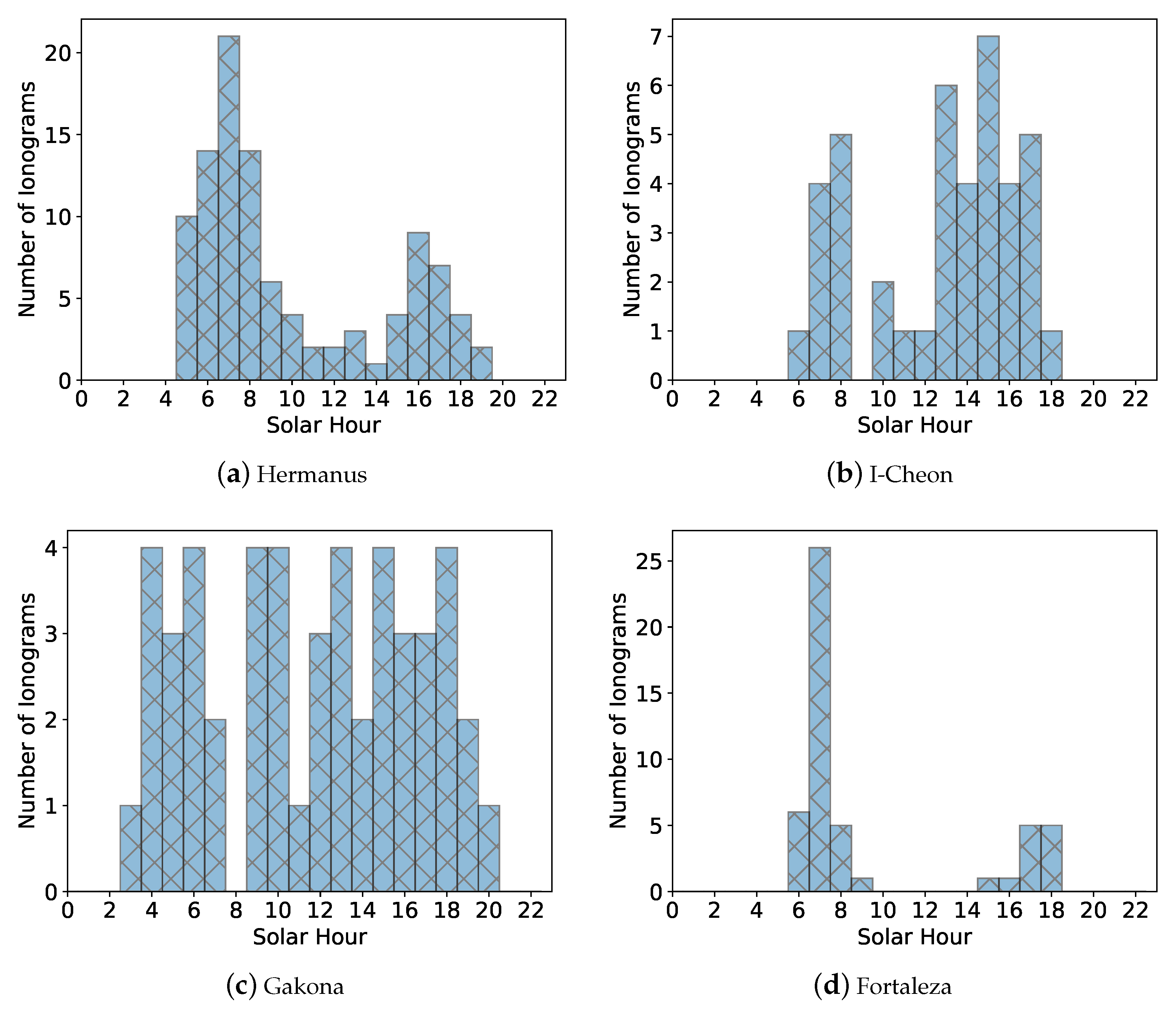
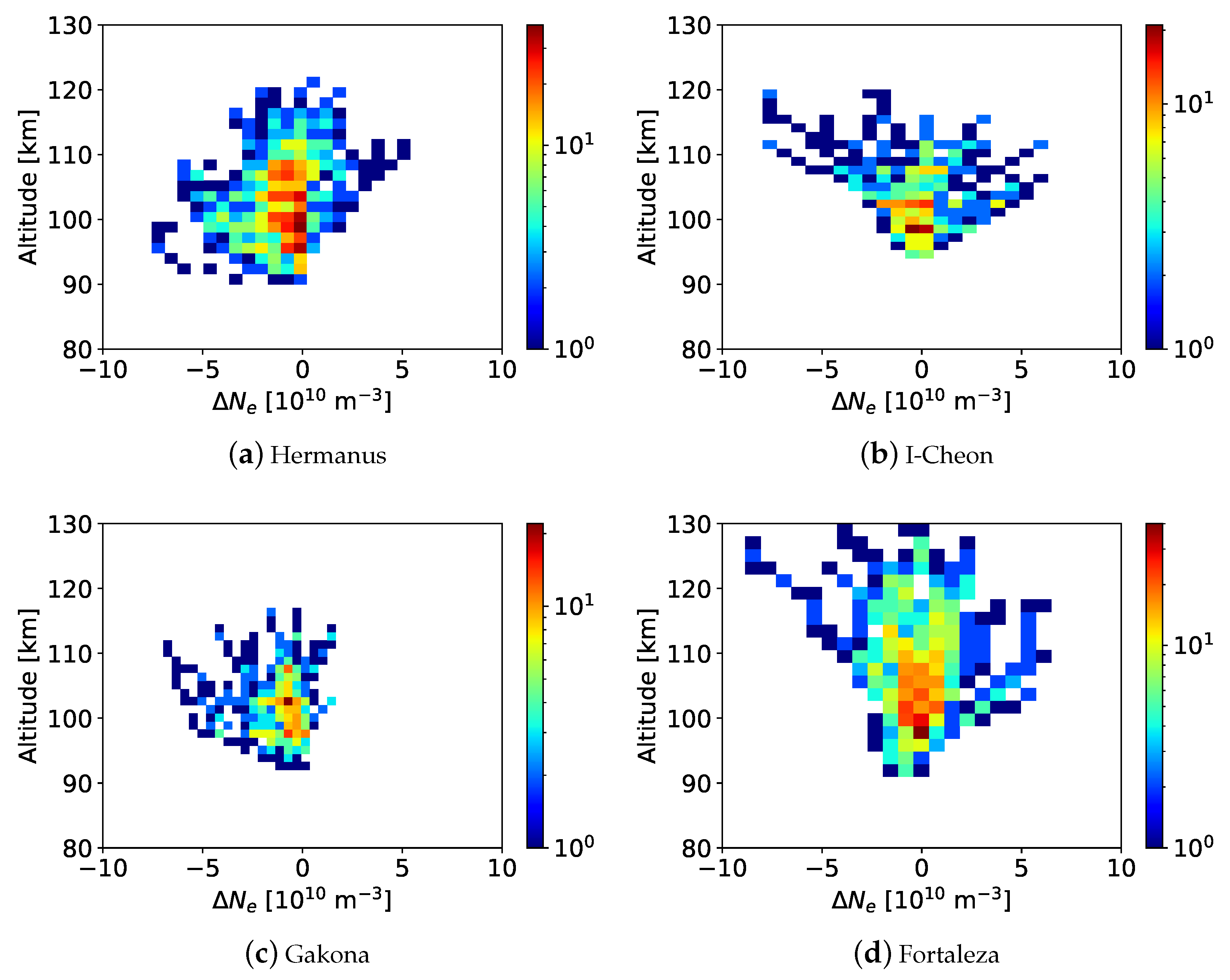
The purpose of this research is to perform an in-depth comparison of the bottom-up method with ionosonde measurements and Faraday-International Reference Ionosphere (FIRI)-modeled profiles at four sites over a wide latitude range: Fortaleza, Brazil, in the equatorial region; Hermanus, South Africa and I-Cheon, South Korea, in the mid-latitude region; and Gakona, Alaska, in the polar region. GNSS-RO profiles are compared against ionograms within 2° and 30 min of the occultation that showed a clear E-region with no sporadic-E ($E_s$) present, and also with FIRI model-generated profiles. EDPs and virtual heights are analyzed to compare and contrast the different remote sensing methods and to provide insight into future improvements for both GNSS-RO and ionogram inversion techniques.

2. Materials and Methods

The primary purpose of this research is an in-depth comparison building on the brief initial comparison outlined in [23] to four sites covering a wide range of latitudes. From the equatorial region, Fortaleza, Brazil (FZA0M, 3.9°S, 321.6°E), was used over the time period October 2019–September 2021. From the mid-latitudinal regions, I-Cheon, South Korea (IC437, 37.1°N, 127.5°E), over the time period June 2010–April 2014, and Hermanus, South Africa (HE13N, 34.4°S, 19.2°E), over the time period July 2008–April 2014 were used. Gakona, Alaska (GA762, 62.4°N, 215.0°E) was used over the time period April 2007–April 2014 in the high latitudes. These dates were selected based on availability of GNSS-RO data in addition to the desire for low minimum frequencies, fmin, measured by the ionosondes. By selecting sites from each latitude zone, a comparison of the GNSS-RO method performance in different regions was possible.

2.1. GNSS-RO Bottom-Up Approach

GNSS-RO profiles were calculated using the COSMIC Data Analysis and Archive Center’s (CDAAC) 50 Hz atmPhs files [24]. Following [23], the first step of the bottom-up approach is the calculation of the horizontal total electron content (hTEC) using both the L₁ and L₂ excess phase. The inclusion of both L₁ and L₂ allows for the removal of the neutral atmosphere contribution to the phase, which follows an exponential relationship with respect to altitude. After the hTEC is calculated, a linear fit to the hTEC as a function of altitude is performed over the altitude range of 30–60 km. The linear phase profile in this altitude range corresponds to the F-region hTEC contribution, as the local electron density is essentially zero at these low altitudes.

Removing this F-region contribution provides ΔhTEC, which allows for estimates of D- and E-region electron densities by effectively reducing the F-region “noise” in the phase profiles. Weighting functions for this ΔhTEC have a much smaller reliance on higher altitudes than the Abel functions, providing a more localized dependence [22,23]. The ΔhTEC profiles are subsequently inverted to provide electron densities as a function of altitude (EDPs). For this inversion, the optimal estimation method [25] is implemented with a reference electron density profile composed of the 2008 annual mean from IRI-2016 [26] for the F-region and FIRI using solar minimum conditions for the E- and D-regions. While the bottom-up approach is helpful for removing the F-region contributions in the lower ionosphere, the extrapolated linear fit can produce large uncertainties at F-region altitudes. Therefore, this method is generally recommended for use at altitudes below 150 km.

The optimal estimation method provides an altitude dependent uncertainty, as displayed in Figure 1. Here, we see the electron density uncertainty increases with altitude from ∼$1\times {10}^9$ m⁻³ at 70 km to ∼$6\times {10}^9$ m⁻³ at 100 km. Additional quality indices are also used to help remove poor profiles, such as the standard deviation of the phase noise in the altitude range of 50–55 km. As displayed in the bottom-right of Figure 1, a phase noise threshold of 0.005 m is used to eliminate poor profiles. Another quality index is based on the electron density ${\chi }^2$ at an altitude of 80 km, which can estimate ionospheric impacts to the neutral atmosphere at lower altitudes (the so-called residual ionospheric effect, RIE). However, this ${\chi }^2$ index does not strongly correlate with poor electron density profiles in the E-region.

GNSS-RO derived EDPs were compared against ionosonde derived EDPs when the occultation was within 2° of the ionosonde location and within 30 min of the ionogram time. Before matching the RO crossings with ionograms satisfying the comparison criteria (outlined in the next section), the total number of occultations within the 2° regions during the periods of interest for each site were: 2162 for Fortaleza, 1402 for I-Cheon, 1739 for Hermanus, and 1403 for Gakona.

2.2. Ionograms

The target minimum frequency measured for ionograms, fmin, was 1.2 MHz or less so that the E-region and its peak would be clearly visible during the daytime. A frequency of 1.2 MHz equates to an electron density of $1.8\times {10}^{10}$ m⁻³, well under the average density of the daytime E-region peak [27]. Thus, ionosondes with fmin at or below this level should detect much of the E-region structure. However, for Gakona and I-Cheon, there were a limited number of ionograms that met this fmin requirement and aligned with an available GNSS-RO profile. As a result, the fmin threshold was increased to the lowest point which provided enough ionograms to be statistically significant. The fmin thresholds and corresponding $N_e$ for each site are displayed in

Table 1. The fmin threshold and electron density corresponding to the plasma frequency fmin for each site. The average E-region peak during the daytime is on the order of 10¹¹ m⁻³, thus the daytime E-region is measurable using these thresholds.

Site	Hermanus	I-Cheon	Gakona	Fortaleza
fmin (MHz)	1.2	2.0	1.2	1.4
$N_{e,fmin}$ (m−3)	1.8 × 1010	5.0 × 1010	1.8 × 1010	2.4 × 1010

. The typical sounding cadence for Digisondes is every 15 min, which was followed by Hermanus. However, I-Cheon followed a 7.5 min sounding cadence, Fortaleza used a 10 min cadence, and Gakona had a variable cadence (all under 15 min). In the event that multiple ionograms met the fmin threshold and were taken within 30 min of a GNSS-RO measurement, the ionogram closest to the GNSS-RO time was used.

Ionograms were retrieved using the SAO Explorer to access data from the Global Ionospheric Radio Observatory (GIRO) [8]. The ionograms were hand-scaled to filter out soundings when the E-region was not measured, or when Sporadic-E ($E_s$) was present, and to ensure low-quality data were removed. For this comparison, the key interest was the new bottom-up method’s performance given a calm ionosphere. Therefore, instances in which $E_s$ was present were excluded. Excluding ionograms that did not have a clear E-region during the hand-scaling process naturally filtered out measurements taken at night. While hand-scaling allows for manual adjustment of the ionogram virtual height traces, the same inversion process used in Automatic Real-Time Ionogram Scaler with True Height calculation (ARTIST) to calculate real heights from virtual heights [28,29] is used for the hand-scaled ionograms.

As displayed in Figure 2, a non-uniform time distribution is produced for each of the sites, with no ionograms at night, and the majority of ionograms during the morning and evening periods. This time distribution is primarily limited by the low fmin thresholds (Table 1), which are mostly satisfied during the morning and evening periods. The limited dataset from this non-uniform time distribution may introduce an additional bias into the comparison, as discussed further in Section 4.

While the optimal estimation method used for the GNSS-RO bottom-up approach naturally provides an uncertainty, it is more difficult to obtain electron density uncertainties from manually scaled ionogram inversions in SAO Explorer as they are not a direct output. While a measure of uncertainty is provided by ARTIST confidence scores [30,31], it is not clear how these confidence scores map to an uncertainty in electron density as a function of altitude. ARTIST-5 has the ability to provide electron density error bars after error histograms are calculated, but these errors are more associated with the difference between automatically and manually scaled ionograms [32], which does not directly apply to this study which uses solely manually scaled ionograms.

Some general electron density uncertainties are provided in the literature for ionogram inversion at E-region altitudes. The authors of [29] provide an foE uncertainty of $\pm 0.3$ MHz (∼$1.1\times {10}^9$ m⁻³), which is lower than the 100 km uncertainty from the GNSS-RO estimates using the bottom-up approach. However, as noted in [33], the assumption of a parabolic shape for E-region Chapman layers rapidly becomes poorer at distances larger than half the scale height away from the E-region peak. This means that the ionogram EDP estimates for this study are most accurate near foE, and have larger uncertainties at lower altitudes. Interestingly, this is the exact opposite trend in uncertainty that is observed for the GNSS-RO EDP estimates.

2.3. FIRI

In addition to comparing the GNSS-RO profiles with ionograms, they were also compared against corresponding FIRI-2018 modeled profiles. FIRI was created as an improved empirical model of the lower ionosphere using rocket-borne wave propagation experiments [34]. Further, all altitudes are treated independently in the model and analytic expressions are derived for neutral density levels instead of altitude. The Faraday rotation measurements from rocket-borne experiments used to create FIRI result in a substantial improvement in electron density estimates at D-region altitudes compared to the standard International Reference Ionosphere (IRI) [34,35]. Further incoherent scatter radar (ISR) comparisons with IRI and FIRI found closer agreement with FIRI predictions of the lower ionosphere [36,37], which motivated our use of FIRI instead of the commonly used IRI.

The inputs for FIRI are the day-of-year (1–365), solar zenith angle (0°–130°), geographic latitude (0°–60°), and the solar F10.7 index in solar flux units (75–200) [35]. The solar zenith angle was calculated using latitude and local solar time for each ionogram, and the F10.7 data were retrieved from NASA OMNIWeb [38]. If the observed F10.7 value was less than 75 or greater than 200, then 75 or 200 respectively was used as they are the limits of the input. The latitude input for FIRI requires positive values. To account for the southern hemisphere locations, the absolute value of latitude is used, and six months must be added to the day-of-year input. Finally, FIRI is focused on non-auroral zones, so it has a maximum latitude of 60°. Since Gakona is above this latitude, 60° was used, and the FIRI profiles may not be representative at this location.

2.4. Ray Tracer

For GNSS-RO virtual height calculations, the EDPs were input to Another Ionospheric Ray Tracer (AIRTracer; a model developed by Eugene Dao at the Air Force Research Laboratory) to calculate ordinary-mode ray paths. The AIRTracer model is based on the Jones-Stephenson [39] formulation using the Booker quartic with no collisions, but re-implemented for computational efficiency in a modern code base. Since the EDPs are only specified at one location and the numerical ray tracer requires three dimensions, we assumed a constant EDP over the area surrounding each ionosonde site. In other words, we have ignored ionospheric tilts that may be present during the ionogram and GNSS-RO measurements. The ray tracer group paths were then used to calculate virtual heights for the E-region ionosphere so they could be directly compared against measured virtual heights from ionosondes.

3. Results

3.1. Individual Electron Density Profile Comparison

In this section, we compare the electron density profiles (real heights) derived from GNSS-RO, ionosonde, and FIRI estimates. Initially, each individual GNSS-RO profile was compared with the corresponding ionosonde and FIRI profiles. The number of profiles used at each site is listed in

Table 2. The number of individual profiles compared for each site. Each GNSS-RO profile is compared against an ionosonde within 2° and 30 min of the profile time, and with an FIRI profile corresponding to the same local solar time and latitude. A total of 208 profiles were compared.

Site	Hermanus	I-Cheon	Gakona	Fortaleza	Combined
Number of Profiles	71	41	49	47	208

. To focus on the D- and E-regions, EDPs are analyzed up to a maximum altitude of 130 km. An example of an individual profile comparison for each site can be seen in Figure 3, where the ionosonde profile is a blue dot-dash line, the GNSS-RO profile is a red dotted line, the FIRI profile is a solid cyan line, the fmin value from the ionogram is included as a vertical black dashed line, and the comparison altitudes are denoted by green markers on the ionosonde profile. These altitudes are the altitudes of the ionosonde profile that occur between the fmin altitude and the altitude of the E-region peak (hmE) and will be used to compare the ionosonde $N_e$ at each given altitude to the corresponding GNSS-RO $N_e$ value at that altitude. The provided GNSS-RO profiles have a 1 km vertical resolution [23], while ionosondes typically transmit with a frequency resolution of 100 kHz [7,32] to obtain virtual heights that are inverted to provide EDPs with a 1 km vertical resolution using SAO Explorer. Since the RO altitudes and ionosonde real heights do not always align, the ionosonde EDPs are interpolated at the RO altitudes using a cubic spline (green markers in Figure 3).

Among all of the individual profiles, there are two key features that are immediately apparent. First, the shape of the GNSS-RO profile in the E-region appears to be very similar to the ionosonde in this region; however, there is a separation of a few kilometers between the two. In the four examples above and nearly all of the individual profile comparisons, the GNSS-RO profile is at a slightly higher altitude at fmin than the ionosonde. The second key feature is the difference in the profile shapes below the ionosonde fmin where the RO profiles show a gradual decrease in electron density between the E- to D-region, where the ionosonde profiles drop rapidly to zero before reaching D-region altitudes. This difference will be discussed in more detail in Section 4.

To account for a potential altitude bias between the GNSS-RO and ionosonde profile, the choice was made to shift one of the profiles so the profiles align at fmin. Since there is some level of uncertainty in the altitude of both the GNSS-RO and the ionosonde profiles, particularly the starting altitude, the ionosonde profiles were shifted. Here, we shift the profiles strictly to compare the EDP shapes, and we do not imply that all ionosonde derived EDPs require a shift in altitude. A more detailed discussion regarding this altitude bias is provided in Section 4.

The altitude shift consists of calculating the altitude difference between the two profiles at fmin and shifting the entire ionosonde profile by the difference, thus pinning the profiles together at fmin. GNSS-RO profiles were not shifted in altitude, such that the ionosonde and RO profiles perfectly align at the fmin altitude. The average distance the profiles were shifted (i.e., the average altitude difference at fmin) is displayed in

Table 3. The average and standard deviation of the altitude difference (Δalt) at fmin for each site and for the combined results. The altitude difference at fmin was calculated for each profile and was used to shift the entire ionosonde profile. Positive values indicate the ionosonde profile was shifted up in altitude.

Site	Hermanus	I-Cheon	Gakona	Fortaleza	Combined
Δalt avg (km)	2.8	4.5	3.9	3.3	3.5
Δalt stdev (km)	5.4	3.5	1.8	2.7	4.1

. Examples of the shifted profiles are presented in Figure 4, which are the shifted profiles corresponding to the examples given in Figure 3.

Once the ionosonde profile has been shifted, the GNSS-RO profiles are nearly the same in the E-region, and the difference in $N_e$ below fmin between the ionosonde and the GNSS-RO profile is much more apparent. Another noteworthy feature of the GNSS-RO profiles that will be discussed in more detail in Section 3.3 and Section 4 is the lack of a clear E-region peak in many of the profiles. This is observed in the Gakona RO profile in Figure 3 and Figure 4, where the profile shows a minor change in slope with respect to altitude near 110 km, but it does not show a clear E-region peak or E- to F-region valley.

All following statistical comparisons aside from the frequency of the E-region peak (foE) and hmE comparison will be performed for both the original unshifted profile and the shifted profile. In Section 3.5, the direct virtual height measurements from the ionosondes are used to compare against virtual heights calculated from the RO profiles, which removes the uncertainty in the ionogram inversion process and eliminates the need to shift profiles for comparison.

3.2. Average Electron Density Profile Comparison

The average EDPs were calculated by first finding the average $N_e$ in one-kilometer increments from 90 to 120 km for the ionograms and 60 to 120 km for the GNSS-RO profiles. The lower thresholds were chosen in order to encompass the minimum altitude for each profile, generally 90 km for ionograms and 55–60 km for the GNSS-RO profiles. The upper threshold of 120 km was selected due to the fact that some of the GNSS-RO profiles have a maximum altitude slightly lower than 130 km. This 120 km encompasses all GNSS-RO profiles and is well above the average hmE. The average $N_e$ for each altitude value was calculated using $N_e$ measurements from each profile corresponding to that altitude. Due to the relatively small number of profiles for each site, the average EDP could not be calculated separately for season, time-of-day, etc., and here we show the overall average for all conditions. However, the standard deviation of these values was calculated for each altitude in the same range to estimate variability and uncertainty.

Figure 5 shows the average GNSS-RO and ionosonde derived EDPs for Hermanus. For the unshifted profiles, the ionogram $N_e$ is larger than the GNSS-RO profiles in the primary area of interest between fmin and hmE. The ionosonde estimates have more variability, as seen by the width of the error bars, but have a clear average E-region peak at 106 km, above which the $N_e$ is almost constant with altitude. In contrast, the RO profiles show a steady increase in electron density with respect to altitude above hmE, which is due to the large number of profiles without a clear E-region peak. In the shifted average EDP, the profiles align better. However, the RO profile remains slightly higher in altitude in most of the region of interest. In both cases, it is clear to see the ionosonde profile $N_e$ rapidly decreases to zero below fmin, while the GNSS-RO profile measures the D- to E-region transition.

Figure 6 shows the average EDPs for I-Cheon. There is less variability in both the average ionosonde and GNSS-RO EDPs due to the fact that there were significantly fewer profiles used for the comparison (the fewest of all the sites). There is a clear average E-region peak at 105 km for the ionosonde, with a nearly vertical density profile above hmE. Of note, the $N_e$ at the average hmE is higher for I-Cheon than it is for Hermanus, both of which are mid-latitude sites. Once the profiles are shifted, the average profiles align closely from fmin throughout most of the E-region, but they begin to diverge near hmE. The GNSS-RO average EDP does not have a clear E-region peak, and density steadily increases in altitude whereas the ionosonde profile begins to increase slowly with altitude up to hmE. This is due to the fact that the E-region peak was not evident in the majority of the GNSS-RO profiles for this site. The shifted ionosonde EDP also appears to be better aligned with the GNSS-RO below fmin; however, this comes from only a few of the profiles having $N_e$ measurements below 90 km. Once the profile is shifted, these are now above 90 km, thus they appear in the calculation for average density.

Figure 7 shows the average EDPs for Gakona. The GNSS-RO profiles generated at Gakona were the least aligned on average of the four sites, with the ionosonde densities larger than the RO densities at all altitudes above fmin. The average ionosonde profile has a flat E-region with a sharp increase in $N_e$ with altitude from fmin to hmE. The GNSS-RO profiles were better at showing an E-region peak than at all other sites, with a nearly vertical average profile at a higher altitude and slightly lower $N_e$ than the ionosonde profile. The average altitude shift was the second largest at 3.9 km, and once shifted, the average EDPs are only well aligned for a small range above fmin. The GNSS-RO profiles gradually increase in altitude as $N_e$ increases, whereas the ionosonde profile is much flatter. Despite the shift, there is still a large separation between the profiles near hmE.

Finally, Figure 8 shows the average EDPs for Fortaleza. Unlike the previous sites, Fortaleza was the only site where the standard deviation of the GNSS-RO profiles was larger than the ionosonde profiles. Additionally, the average ionosonde profile has a more gradual increase in $N_e$ with altitude than the average ionosonde profile at the other sites and still has a positive slope above average hmE. The GNSS-RO $N_e$ is larger than the unshifted ionosonde $N_e$ at hmE, also unlike the other sites. In the comparison with the shifted ionosonde profile, the average EDPs show reasonable agreement from fmin for the lower part of the E-region but have a large separation in $N_e$ at hmE. The GNSS-RO profile gradually increases and does not have a clear E-region peak in the average profile.

An average EDP comparison was also performed for each site between the GNSS-RO and FIRI average profiles. The shifting process was only performed for comparisons with ionosondes; thus, there is only one comparison for each site between the GNSS-RO and FIRI, shown in Figure 9. The average fmin and unshifted hmE measured by the ionosondes for each site are included for reference.

The GNSS-RO and FIRI average EPDs are similar for each site, thus they will all be discussed together. Unlike the ionosonde profiles, the average FIRI profiles are slightly higher in altitude than the GNSS-RO profile. It is clear to see from the shaded FIRI standard deviation area ridge in altitude below fmin that there are profiles with either a double ledge or a ledge below fmin. This ridge is least prevalent at I-Cheon and occurs most prominently at Gakona and Fortaleza. The variability between the GNSS-RO and FIRI profiles at Gakona and Hermanus is low. However, the GNSS-RO profiles at I-Cheon and Fortaleza are at a lower altitude than the FIRI and have a large separation in $N_e$ at hmE. The GNSS-RO profiles are in good agreement overall with Hermanus and Gakona, with little separation between the profiles from fmin to hmE, and show poorer agreement at Fortaleza and I-Cheon. The key takeaway from the comparison with the FIRI profiles is the performance at relatively low electron densities and altitudes, with a strong agreement in the D- to E-region transition at all sites.

3.3. foE and hmE Comparison

The E-region electron density peak, foE, and corresponding altitude, hmE, for GNSS-RO and ionosonde profiles were compared next. These values were extracted directly from the ionograms and were estimated for each corresponding GNSS-RO profile through visual inspection of the EDPs. For this comparison, only the hmE from the unshifted ionosonde profiles was used. Due to the smoothing nature of the optimal estimator algorithm and the one kilometer vertical resolution, some of the GNSS-RO profiles did not have a clear E-region peak (to be discussed in more detail in Section 4). In these cases, the profile was excluded from the foE and hmE comparison. The number of profiles used for each site and for the combined comparison is shown in

Table 4. The number of profiles used for foE and hmE comparison for each site. Many profiles had to be removed, particularly at I-Cheon and Gakona due to GNSS-RO profiles without a clear E-region peak.

Site	Hermanus	I-Cheon	Gakona	Fortaleza	Combined
Total Profiles	71	41	49	47	208
foE and hmE Profiles	55	14	26	36	131

.

GNSS-RO and ionogram foE values are displayed in Figure 10 for all four sites. Due to a large percentage of GNSS-RO profiles at I-Cheon without a clear E-region peak, there were not enough profiles for a statistically significant comparison. While the figures for I-Cheon are included, the discussion will focus on Hermanus, Gakona, and Fortaleza.

At each site, the foE between the two profile methods are generally spread around the 1:1 line with slopes near one. The average foE of the GNSS-RO profiles is slightly lower than the ionosonde profiles at Hermanus and Gakona and is virtually the same at Fortaleza (

Table 5. The foE R² and average difference for each site and for the combined results. A negative value indicates the average ionosonde foE is larger than the average GNSS-RO foE, and a positive value indicates GNSS-RO is larger.

Site	Hermanus	I-Cheon	Gakona	Fortaleza	Combined
R2	0.64	N/A	0.43	0.33	0.58
Avg. ΔfoE (MHz)	−0.07	0.04	−0.12	0.02	−0.05

). There is relatively large variability in foE for both the GNSS-RO and ionosondes, which leads to lower R² values despite the linear fit having nearly the same slope at all sites.

A cumulative distribution function (CDF) histogram for the difference between the values was calculated and is shown in Figure 11. The foE difference was calculated by subtracting the ionosonde foE from the GNSS-RO foE, and the CDF histograms produced similar results for all sites. Hermanus has a slight negative skew at one standard deviation, while Gakona has a slight positive skew and Fortaleza is nearly symmetric about the mean. Hermanus and Gakona had three and two profiles with an foE difference greater than 1 MHz, respectively. These sites also have a slightly negative average difference, meaning the ionosonde tends to measure a slightly larger $N_e$ at the E-region peak. For all sites, most profiles have an foE difference within ±0.5 MHz.

The hmE comparison was performed in the same manner as foE, with the hmE values shown in Figure 12. As before, there is not enough data for a statistically significant comparison at I-Cheon, so the figures for I-Cheon are included, but the discussion will focus on Hermanus, Gakona, and Fortaleza.

The GNSS-RO hmE generally do not match well with the ionosonde values. For Hermanus and Gakona the GNSS-RO hmE is found in a narrower altitude range than the ionograms, which is particularly noticeable for cases when the ionosonde hmE altitude is low. As a result, the average hmE is larger for the GNSS-RO profile, as can be seen in

Table 6. The hmE R² and average difference for each site, and for the combined results. Positive values indicate the average GNSS-RO hmE is larger than the average ionosonde hmE.

Site	Hermanus	I-Cheon	Gakona	Fortaleza	Combined
R2	0.30	N/A	0.13	0.24	0.30
Avg. ΔhmE (km)	2.7	6.0	7.4	1.2	3.6

. There were several GNSS-RO profiles that had an hmE close to 100 km which drove the average value down, but nearly all of the profiles at this site had a higher hmE value than the ionogram hmE. The profiles at Fortaleza did not follow this trend, and as a result, the average hmE difference is lower for this site. As with the foE, a CDF was calculated for the difference between the GNSS-RO and ionosonde values and is shown in Figure 13.

All sites have an average hmE difference that was positive, and the standard deviation had a slight negative skew. Of note, the average hmE difference was roughly the same as the average shifted value at each site, meaning if the hmE value had also been shifted, the difference would be close to zero. Fortaleza had the widest spread, with two profiles having an absolute difference greater than 20 km.

3.4. Point-by-Point Electron Density Comparison

Next, the $N_e$ values of the GNSS-RO profiles at each altitude were compared to ionosonde values between the fmin and hmE altitudes. The altitudes of the GNSS-RO and ionosonde profiles do not necessarily match, so the ionosonde $N_e$ is interpolated to the altitudes used in the GNSS-RO profile using a cubic spline. Electron densities for each altitude of the GNSS-RO profile between the fmin and hmE of the ionosonde are shown for each site in the unshifted comparison in Figure 14, and the shifted comparison in Figure 15. Approximately 14 points per profile are used in the comparison within this altitude range for the 1 km vertical resolution of the GNSS-RO profiles. R² and mean absolute error (MAE) values for the shifted and unshifted comparisons at each site are shown in

Table 7. R² and MAE values for the unshifted and shifted $N_e$ for all altitudes between fmin and hmE.

Site	Hermanus	I-Cheon	Gakona	Fortaleza
Unshifted R2	0.66	0.44	0.39	0.54
Shifted R2	0.70	0.59	0.58	0.54
Unshifted MAE (1010 m−3)	1.9	3.0	2.4	1.7
Shifted MAE (1010 m−3)	1.3	1.5	1.4	1.3

.

For the unshifted profiles shown in Figure 14, it is clear that for almost every altitude in all of the profiles, the ionosonde $N_e$ is larger than the GNSS-RO $N_e$. As displayed with the individual and average profile comparisons, the ionosonde profile tends to be at a slightly lower altitude than the GNSS-RO profile. Due to the nature of the E-region ionosphere where $N_e$ is increasing rapidly with altitude, a separation of just a few kilometers can cause a significant difference in $N_e$. Since the ionosonde profile is lower in altitude, at any given altitude it will have a higher $N_e$ than the GNSS-RO profile. Hermanus had the highest R² for the unshifted profiles, and the lowest was at Gakona and I-Cheon. Gakona had the largest difference between unshifted profiles, and I-Cheon had both the largest average fmin and the largest spread in $N_e$ measurements. Fortaleza has the most profiles with data points above the 1:1 line, meaning the GNSS-RO $N_e$ was larger for that point. In general, as $N_e$ increases at higher altitudes, there is a larger variation between the GNSS-RO and ionosonde profiles.

The profiles corresponding to large differences in foE are also displayed in Figure 14. For example, I-Cheon shows two profiles with RO estimates significantly larger than the ionosonde estimates, and a few profiles with ionosonde estimates much larger than the RO estimates. These profiles correspond to the foE differences outside of one standard deviation in Figure 11.

In the comparison for the shifted profiles, shown in Figure 15, the R² is unchanged for Fortaleza and is stronger for Hermanus, I-Cheon, and Gakona. The method for shifting the profiles set the altitude at fmin equal for the GNSS-RO and ionosonde profiles, thus the first $N_e$ value for each shifted profile falls on the 1:1 line. For all of the sites, the linear fit remains a shallower slope than the 1:1 line, meaning that as altitude increases, the ionosonde profile tends to have a larger $N_e$ than the GNSS-RO profile. Fortaleza shows the lowest slope of 0.55, which may be due to ionospheric tilts present during the dawn/dusk measurements. Overall, the GNSS-RO profiles are in good agreement with the shifted ionosonde profiles.

The $N_e$ difference for the shifted profiles is shown in Figure 16. With the profiles pinned at fmin, the $N_e$ difference is zero for all profiles at fmin. The histograms at all sites show a V shape with low variability in $N_e$ between the profiles at low altitudes. Gakona has a slightly negative center, but all other sites are roughly centered at zero. Overall, Hermanus and Gakona have lower variability at all altitudes, with nearly all points having a difference within $5\times {10}^{10}$ m⁻³. I-Cheon and Fortaleza have larger variability at high altitudes, which could also be seen by a relatively low R² value in the scatter plots despite the linear fit having roughly the same slope as the 1:1 line. For all sites at all altitudes, the majority of profiles have a difference close to zero, and the shifted MAE is lower at each location.

3.5. Virtual Height Comparison

The final comparison performed for each individual site was for the virtual height profiles. Virtual heights are directly measured from the ionosondes, which provides a validating dataset for the RO profiles after they are used to calculate a virtual height. The ionosonde predicted electron density profiles are calculated using assumptions about profile shapes, etc. (e.g., [5,40]), which adds additional uncertainty into the estimates. However, the virtual height is a direct measurement and, therefore, provides a direct validating dataset.

GNSS-RO virtual heights were calculated using the numerical AIRTracer model to estimate ordinary-mode (O-mode) group paths for each plasma frequency in the RO profile above the ionosonde fmin. Virtual heights above 140 km were removed to exclude cusps that result in large virtual heights near foE. Examples of the calculated virtual heights along with the measured virtual heights are displayed in Figure 17. In this figure, only the points used for the comparison are displayed, which removes the virtual heights above 140 km and frequencies below fmin. While some of the foE estimates in Figure 17 look incorrect (specifically, Gakona and Fortaleza), this is an artifact of the 140 km limit which removes the large virtual heights near the foE cusp. Further, D-region virtual heights are not calculated for the RO profiles because the ionosonde data are limited to frequencies above fmin.

Extending this procedure to all of the EDPs used in this study provides the virtual height scatter plots displayed in Figure 18. From this, a few trends are immediately obvious. First, there is a clustering of data points near the 1:1 line at low altitudes between ∼100–110 km. This clustering is most obvious for Hermanus, but also present to a smaller extent in I-Cheon and Gakona. As the virtual height is related to the integral of the EDP as a function of altitude, this indicates that many of the RO EDP estimates up to fmin are consistent with the measured virtual heights. However, outlying points also exist for the RO virtual heights within the 100–110 km range of ionosondes, where the RO virtual heights are overestimated by 10 and 30 km. This is most pronounced in the Gakona dataset, but also present at the other sites. Interestingly, Fortaleza only shows the overestimated virtual heights at these lower altitudes and does not show the clustering near the 1:1 line as displayed for the other sites. These outliers are either due to large overestimates of the altitudes for plasma frequencies below fmin, or local peaks (large vertical gradients) in electron density that occurs at these lower altitudes.

The second obvious trend is the increased spread in points at higher altitudes. This increased spread is a result of large virtual heights produced near local density peaks (such as foE), which can occur for both ionosondes and RO profiles. For Gakona and Hermanus, the positive virtual height bias for the RO data indicates that the foE may be too low compared to the actual foE measured by ionosondes, or the hmE can be too high. From the small subset of profiles displayed in Figure 10 and Figure 12, it appears the elevated RO hmE is the culprit, but this should be re-explored with a larger dataset as it could be a combination of the two factors. For I-Cheon and Fortaleza, the positive bias exists at lower altitudes while it switches to a negative bias (RO virtual heights less than ionosonde) at higher altitudes.

The difference between the virtual heights was calculated by subtracting the ionogram heights from the GNSS-RO heights (

Table 8. MAE and R² values for the GNSS-RO and ionosonde virtual heights.

Site	Hermanus	I-Cheon	Gakona	Fortaleza
R2	0.36	0.18	0.19	0.23
MAE (km)	7.6	8.1	11.0	8.4

). Difference histograms and CDFs are displayed in Figure 19, which show all of the sites except Gakona have an average difference around zero. Gakona, however, shows a positive bias of around 7 km. Figure 19 does not split the data into altitude bins as performed in Figure 16 because the difference trends over altitude were not as obvious as the electron density trends.

4. Discussion

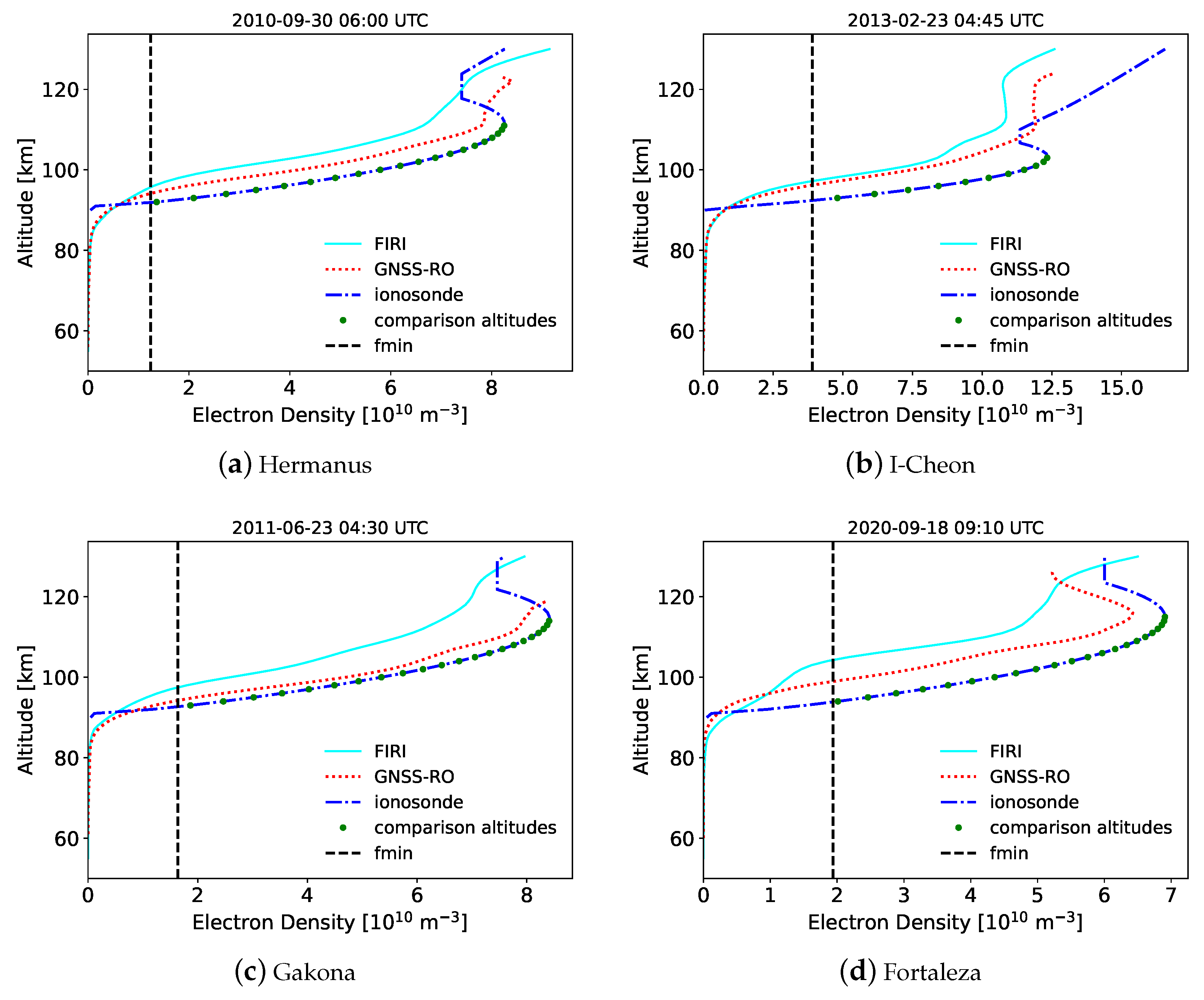
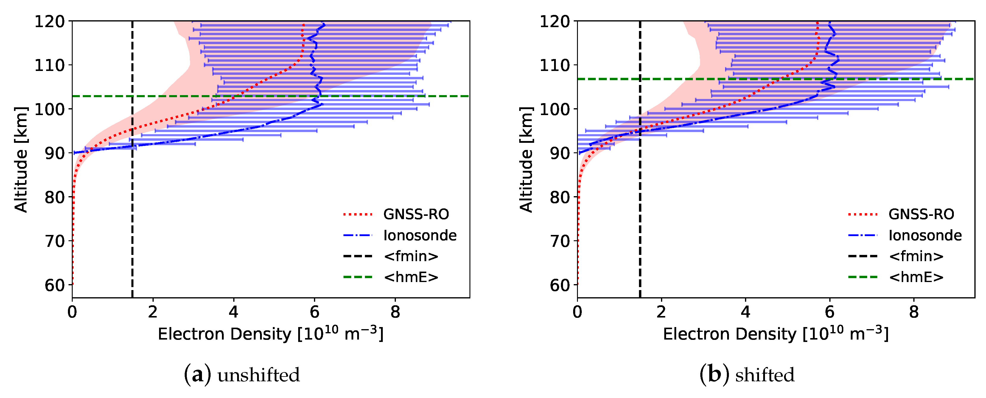
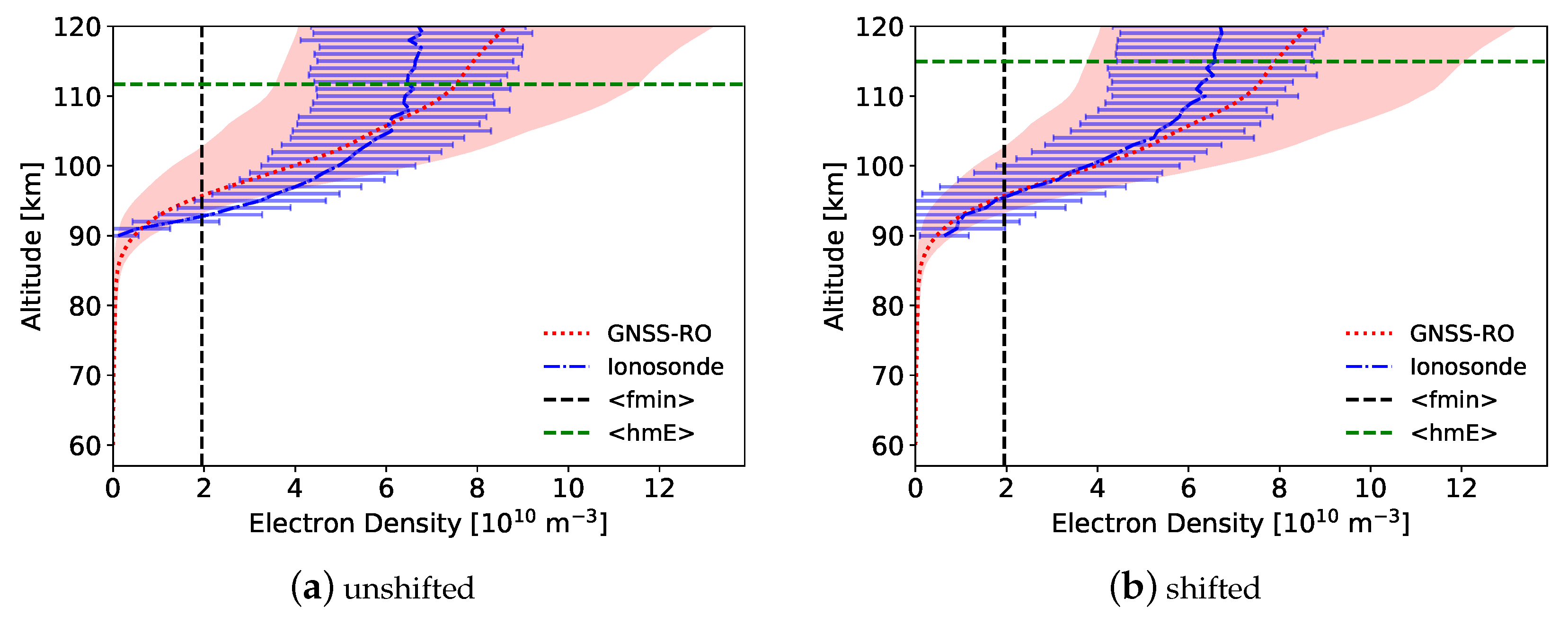
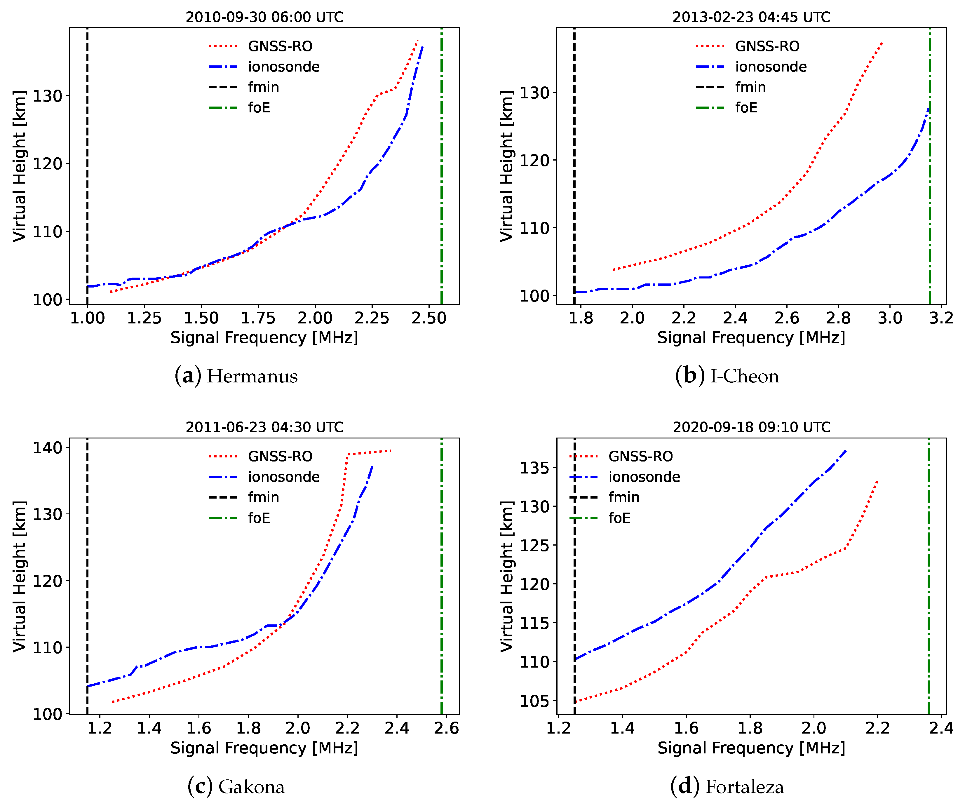
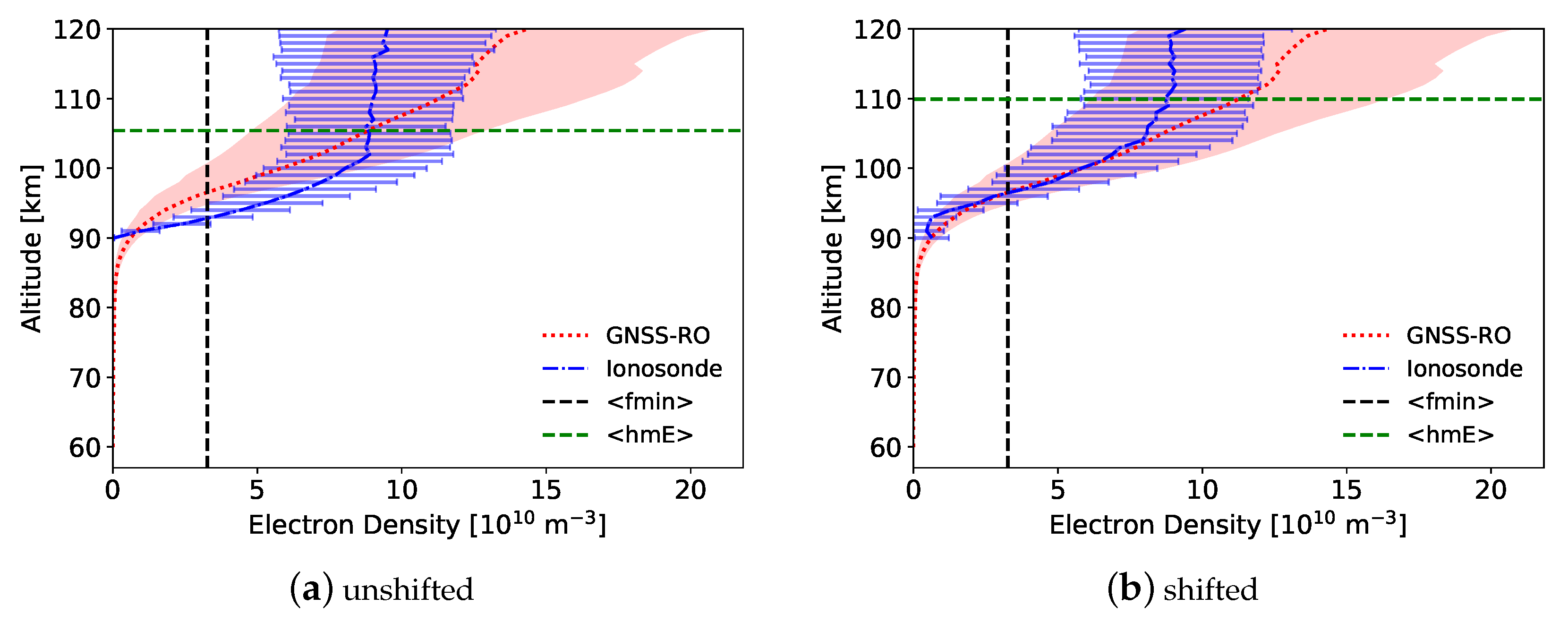
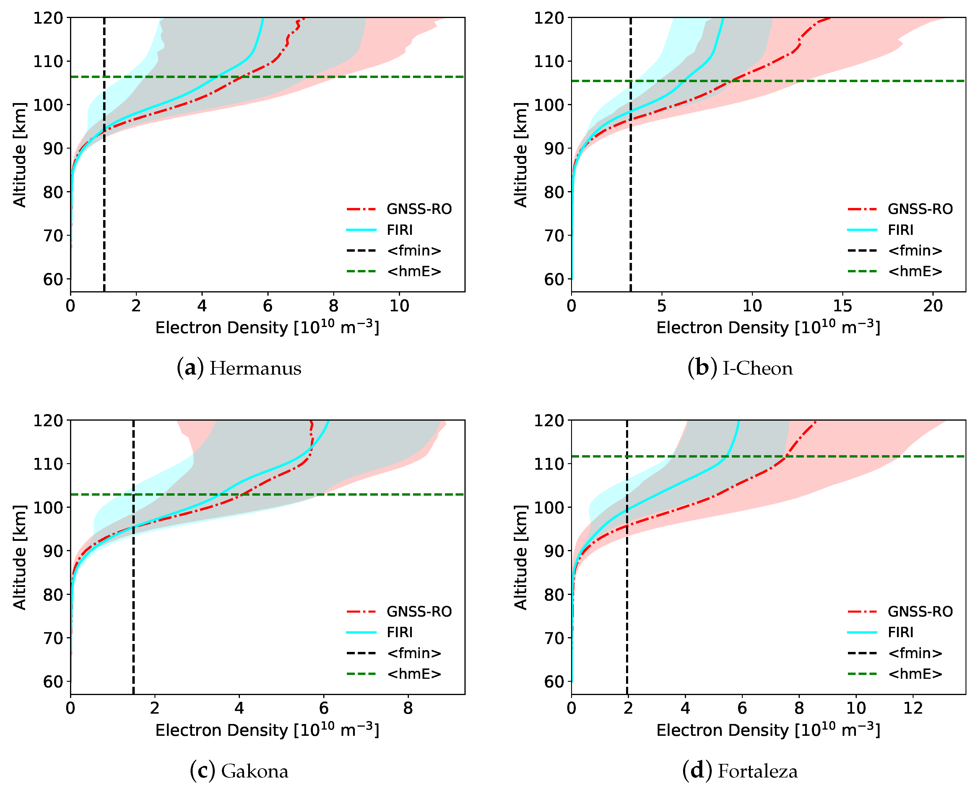
The most obvious difference between the GNSS-RO and ionosonde-derived profiles is the shape of the D- to E-transition region. While the ionosonde EDPs show a sharp decrease from fmin to an electron density of zero, the GNSS-RO shows a smooth transition to the D-region with a greatly reduced but non-zero electron density. This smooth transition is in good agreement with the FIRI profile shapes, which were derived from rocket measurements [35]. Ionosondes do not measure below fmin and make the assumption of a quasi-parabolic shape for the bottomside E-region, thus the $N_e$ rapidly decreases to zero at an altitude close to the fmin altitude [41]. FIRI, however, includes D-region $N_e$ estimates [35] such that $N_e$ is zero at approximately 60 km and slowly increases with altitude up to the E-region where it rapidly increases up to hmE. The GNSS-RO profile has a strong similarity to the FIRI profile shape at these low altitudes, indicating that it is properly measuring the D- to E-region transition and is characterizing the lower ionosphere at electron densities that cannot be measured by ionosondes.

The process used by ARTIST to calculate the real height has uncertainty as to the starting height of the profile [32]. Error can be introduced into the ionogram profiles in several ways, such as non-representative auto-scaling, uncertainty in the region between the E- and F- layers, and the fact that ionosondes are unable to measure below fmin [40]. Additionally, ionosondes calculate real height from the measured virtual height using Chebyshev polynomials, which require some knowledge of the starting height of each layer, and an assumption of a parabolic E-region below fmin [41]. The authors of [42] provide a method for estimating the starting height for the inversion process using the solar zenith angle, a seasonal term, sunspot number, and time after sunset. An in-depth discussion on calculation strategies used by ionograms is provided in [5]. Further, it must be noted that alternative ionogram inversion models, such as POLynomial ANalysis program (POLAN), do not make the same assumptions about the profile shape below fmin [5,43], which may be helpful for studies of the D- to E- transition region.

While there are uncertainties in ionosonde derived EDPs, uncertainties also exist for the GNSS-RO profile altitudes due to ray bending/separation [13] and ionospheric inhomogeneities [17,44,45]. The E-region EDP retrieval from the bottom-up method has the highest data quality at 90–100 km. At lower altitudes it is limited by measurement noise because it removes the F-region contribution using the GNSS-RO profile itself and the E-region EDP contribution decreases exponentially with height. At higher altitudes >100 km, F-region bending and sporadic-E effects are neglected by the bottom-up method. Therefore, the EDP retrieval error is expected to increase at higher altitudes.

Additionally, the optimal estimation method [25] used to invert the GNSS-RO measurements [22,23] is optimized to minimize oscillations in the EDP which may induce biases in foE/hmE estimates. The typical top-down onion peeling method used for RO inversion [46] is known to produce negative electron densities from oscillations near the bottom of the profile [17,47], and the optimal estimation method is able to significantly reduce these negative oscillations through an E-region focused retrieval design and the effective removal of the majority of the F-region contribution (see discussion in [22,23]). However, this places fewer constraints on the densities predicted for the top of the profiles near and above 120 km, which may smooth out the E-layer peak such that the foE and hmE estimates are negatively impacted. Finding the correct weighting balance is critical and is the focus of an ongoing investigation using a larger dataset for comparison that relies on automatically scaled foE and hmE instead of the hand-scaling used in current study.

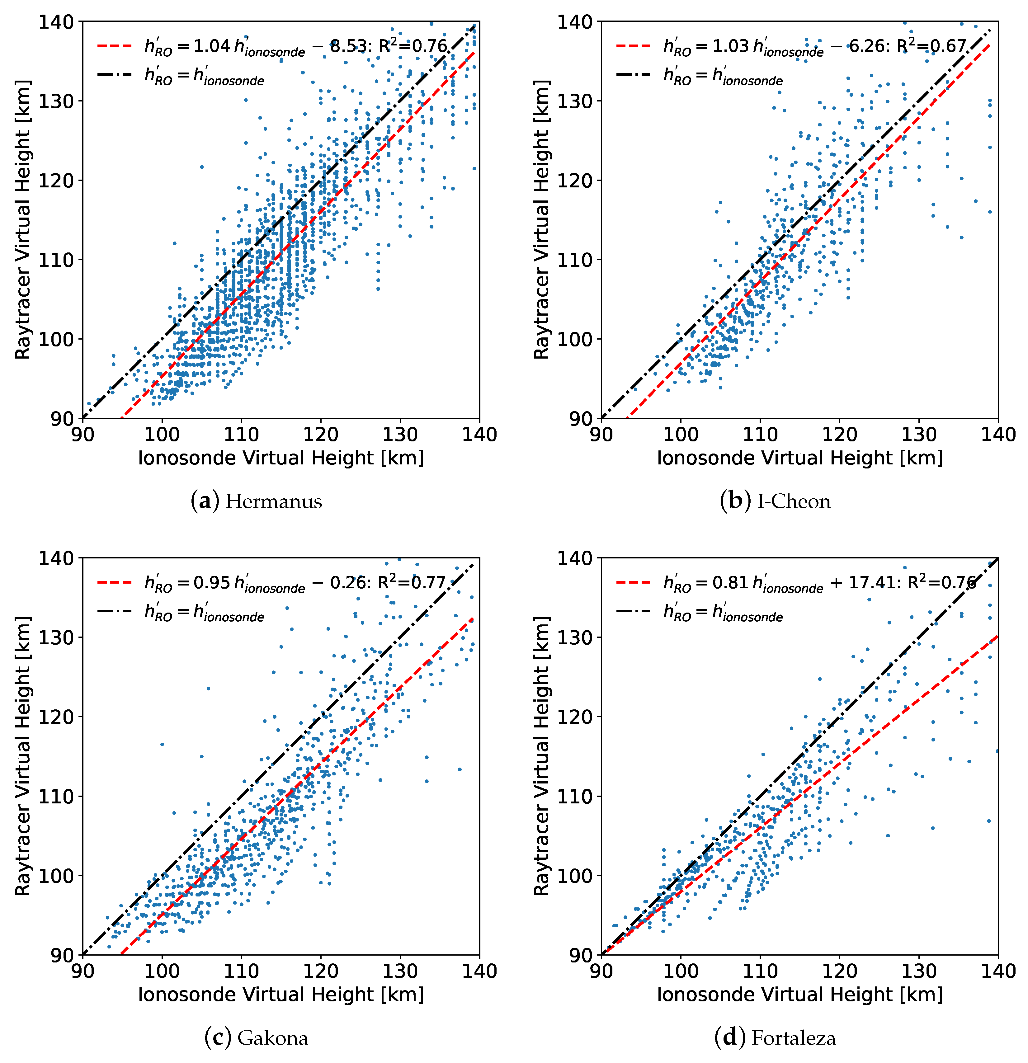
Interestingly, while the electron density profiles show an altitude bias at fmin, the virtual height comparison shows an agreement for many profiles near the lower fmin altitudes (Figure 18). The RO virtual height profiles show a positive bias at lower altitudes due to local density peaks that produce elevated virtual heights, but the mid-latitude sites (Hermanus and I-Cheon) show a clustering near the 1:1 line at the lowest altitudes. Since the ionosonde virtual heights are direct measurements that do not require additional assumptions or processing to interpret, the agreement at lower altitudes suggests that many of the RO profiles are in general agreement with the actual electron density profiles up to fmin. However, this agreement does not match with the persistent altitude bias between ionosonde and RO EDPs at fmin, which motivated us to analyze the ionosonde EDPs using the same AIRTracer used to calculate RO virtual heights.

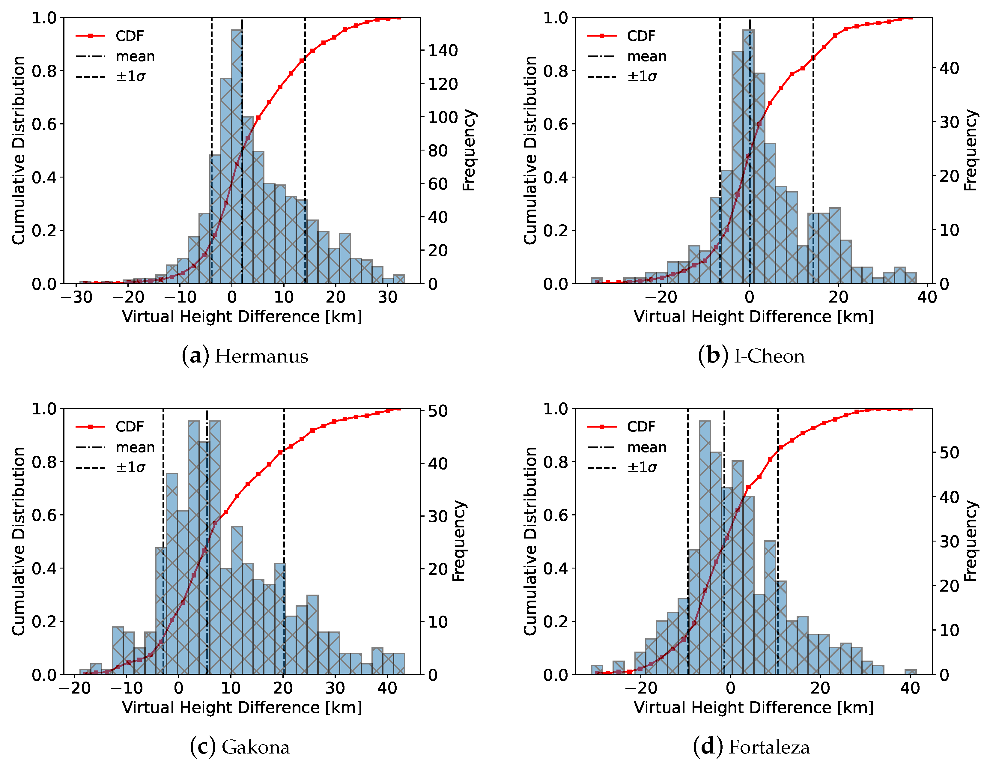
Following the same procedures as described for the RO virtual heights surrounding Figure 18, virtual heights were calculated from the ionosonde EDPs to compare against the direct virtual height measurements from the same ionosondes. The results are displayed in Figure 20, which show a negative altitude bias for the virtual heights calculated using the ionosonde EDPs with a numerical ray tracer. Interestingly, the negative bias observed here at the lower altitudes near fmin is similar in magnitude and direction as the bias between the RO and ionosonde EDPs discussed in Section 3.1.

This altitude bias may be an artifact of the quasi-parabolic shape assumption for the E-layer, which results in a slight altitude difference for the observed virtual heights compared to the idealized electron density profiles derived from the measurements. 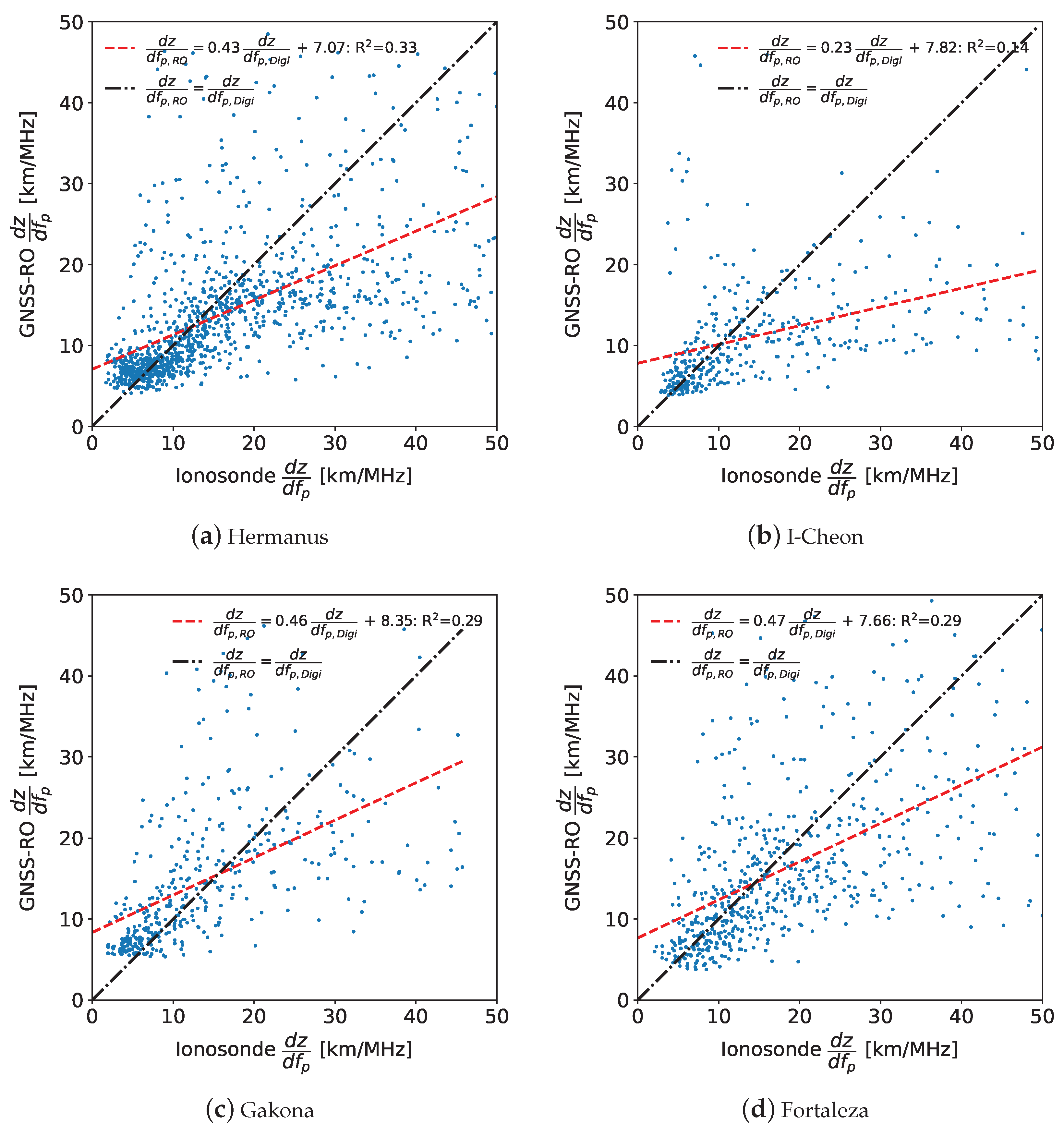As the virtual heights are directly proportional to the integral of the altitude gradient with respect to plasma frequency, $\mathrm{d}z/\mathrm{d}{f}_p$, assumptions on the shape of the E-layer up to foE will impact the derived altitude gradient, which will in turn impact the virtual heights calculated from the electron density profiles. A comparison between the $\mathrm{d}z/\mathrm{d}{f}_p$ calculated for the shifted GNSS-RO and ionosonde profiles is displayed in Figure 21. Interestingly, the GNSS-RO profiles have larger $\mathrm{d}z/\mathrm{d}{f}_p$ for the smaller values, while the ionosonde altitude gradients are larger at elevated values. This indicates that the RO profiles are increasing in altitude more rapidly then the ionosonde profiles at the bottom of the layers near fmin, while the ionosonde profiles increase more rapidly near foE. While the RO profiles cannot be used as a validating dataset here, this difference provides insight into the impacts of the quasi-parabolic shape assumptions that may result in exaggerated $\mathrm{d}z/\mathrm{d}{f}_p$ near foE. These exaggerated altitude gradients allow for the E-layer to be shifted down in altitude to match the virtual height observations, as the virtual height is dependent on the integral of $\mathrm{d}z/\mathrm{d}{f}_p$. A reduction in the altitude gradients would require the profiles to be shifted upwards in altitude, which may help to increase agreement between the ray tracer virtual height estimates and the direct ionosonde measurements.

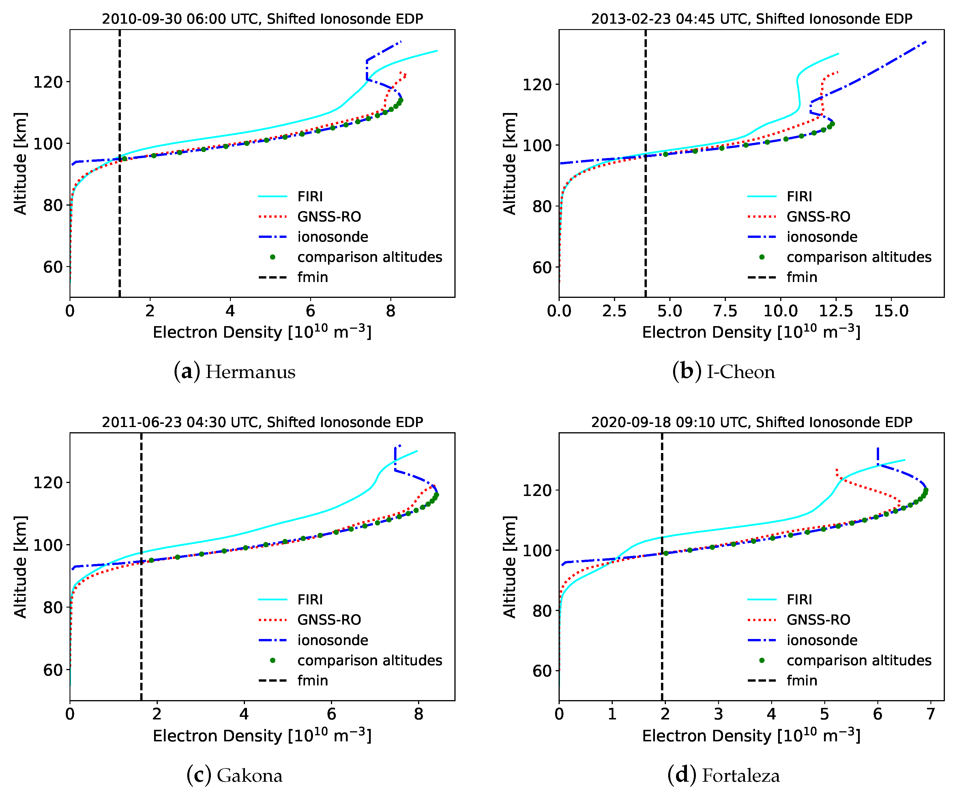
This uncertainty in the virtual height to real height inversion has a direct impact on the EDP comparison. The bias observed between the ray tracer virtual heights and ionosonde observations has the same direction and magnitude as the difference between the GNSS-RO and ionosonde EDPs at fmin (Table 3). Accounting for this potential bias is essentially the same as shifting the ionosonde profiles up in altitude, as performed in Section 3.1 and Section 3.4, which significantly improves agreement between the two approaches for measuring lower ionosphere EDPs. As discussed in [33], the ionosonde EDP uncertainty increases further down in altitude from the E-layer peak given the assumption of a parabolic shape to describe a Chapman layer. From these uncertainties, we believe that the shifted profile comparison is more appropriate for analyzing differences between the GNSS-RO and ionosonde-derived EDPs.

Additionally, we ignored ionospheric tilts using the ray tracer as we only have EDP estimates at a single location. This assumption is not valid near dawn/dusk when large ionospheric tilts are present [48], which is a time period included in our analysis due to the lower fmin values. For sites such as Fortaleza, where almost all of the measurements occur near the dawn/dusk terminator (Figure 2), these ionospheric tilts can be the cause of the altitude differences and biases between the RO/ionosonde EDPs and the direct ionosonde virtual height measurements. Extending this analysis to a larger scale comparison that focuses on foE and hmE would allow for the removal of profiles during the dawn/dusk terminator to determine the impact of these ionospheric tilts on the comparison.

5. Conclusions

A comparison of the bottom-up approach for generating electron density ($N_e$) profiles in the D- and E-region ionosphere created by [22] and refined by [23] was performed. GNSS radio occultation (GNSS-RO) profiles were compared against ionograms at four sites around the world when the occultation was within 2° of the ionosonde location and within 30 min of a sounding that clearly measured the E-region and its peak. Ionograms were hand-scaled to ensure quality and soundings with sporadic-E ($E_s$) were removed from the comparison. The ionosonde sites covered all three the latitudinal regions; Fortaleza, Brazil, in the equatorial region; Hermanus, South Africa, and I-Cheon, South Korea, in the mid-latitudes; and Gakona, Alaska, at high-latitudes. In addition to ionosonde derived profiles, FIRI profiles were also generated for comparison. This comparison was primarily concerned with the E-region with a focus on the region between the minimum frequency measured by the ionogram (fmin) and the height of the E-region peak (hmE).

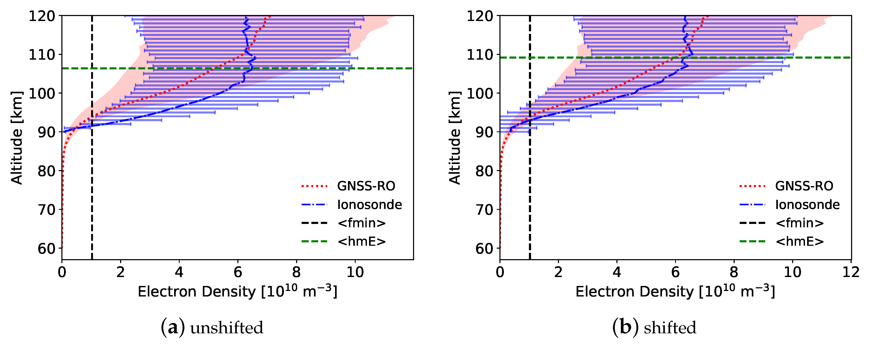
From the comparison, the GNSS-RO and ionosonde EDPs were shown to have similar shapes in the region of interest, but the ionosonde profiles tended to be slightly lower in altitude. There is uncertainty in the EDP altitudes for both the ionosonde and GNSS-RO profiles, thus the altitude difference at fmin was calculated and the profiles were shifted to focus on the profile shapes. The shifted EDPs show generally good agreement. The FIRI EDPs did not align well with the GNSS-RO profile in the region of interest. However, they have a nearly identical shape at lower altitudes below fmin, where the ionosonde follows a parabolic shape to zero $N_e$ based on an assumed shape of the E-region. This agreement between the RO profiles and FIRI below fmin is evidence that the GNSS-RO profiles are capable of measuring the D- to E-transition, which is not possible from ionosondes.

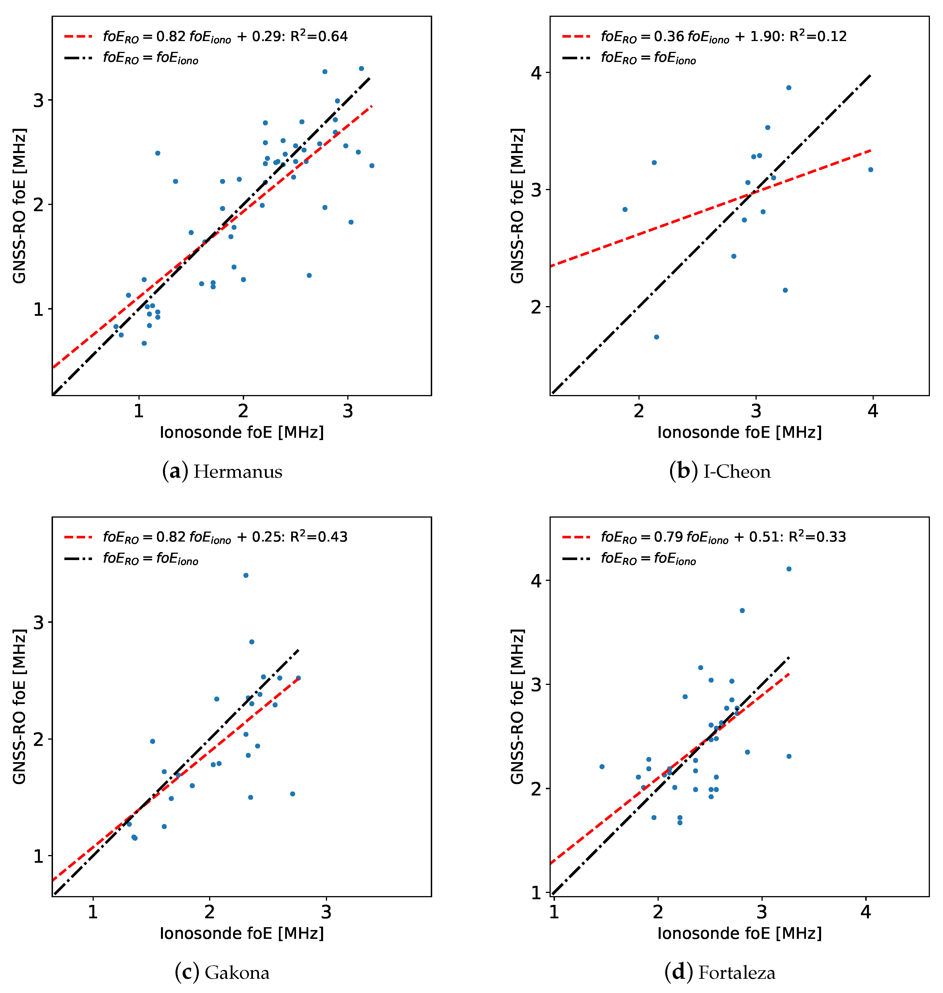
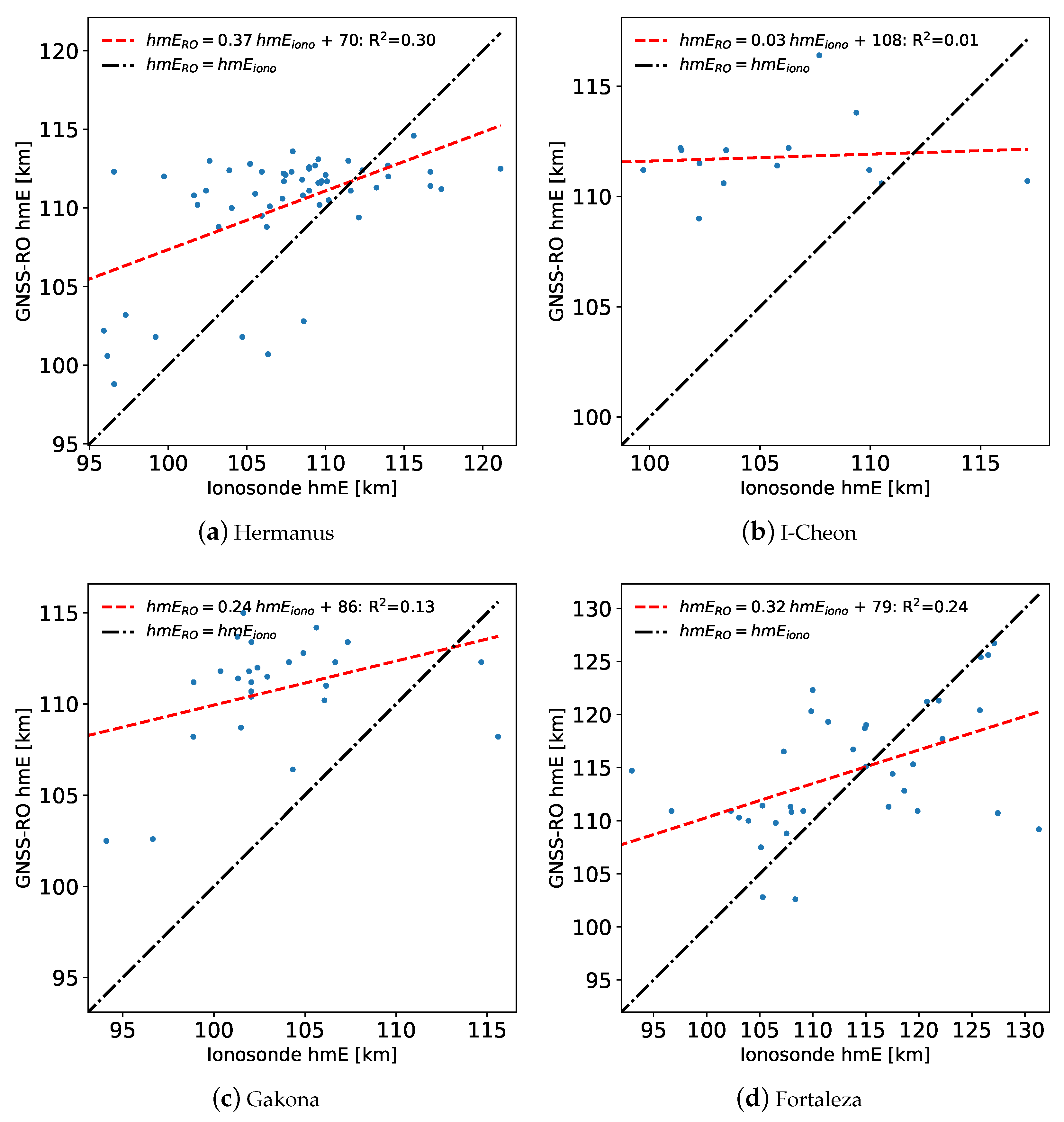
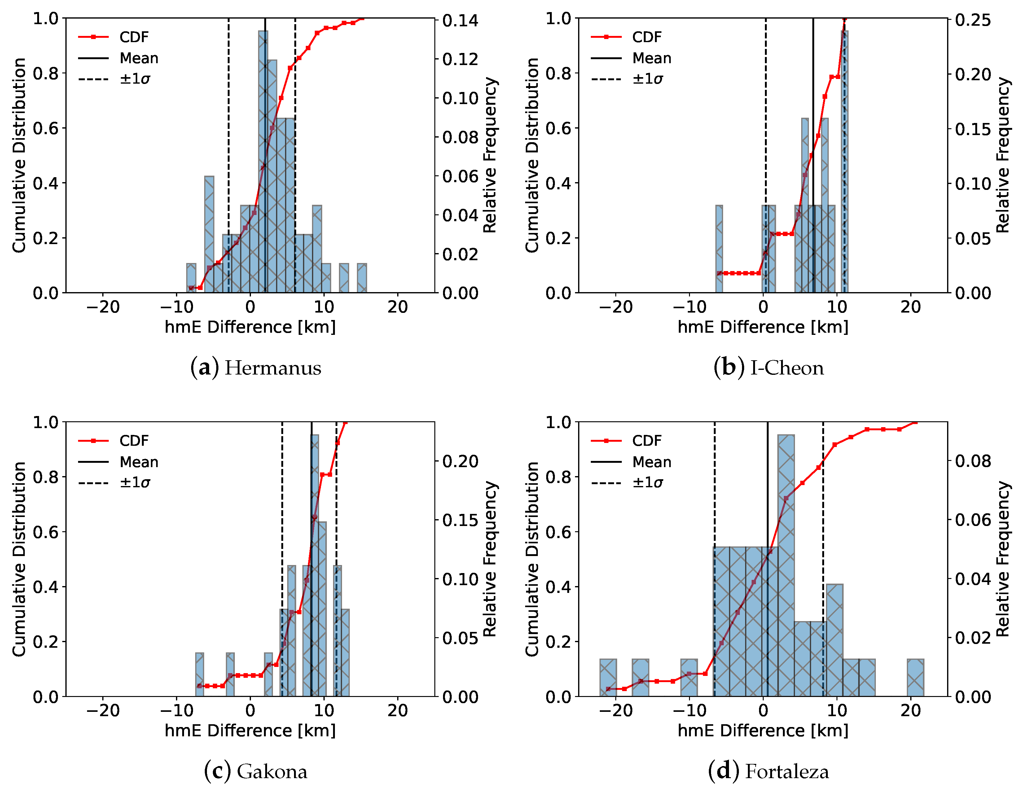
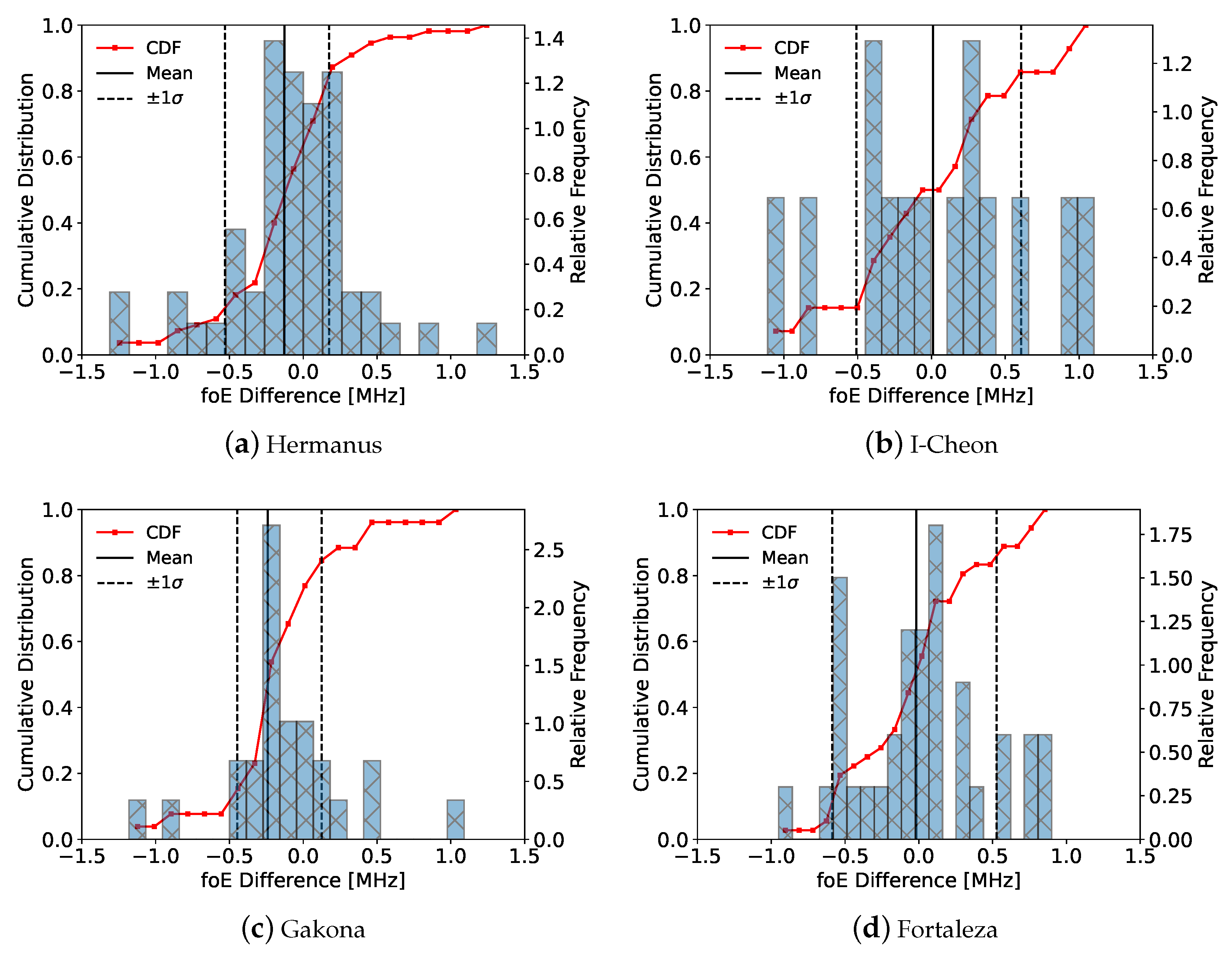
Ionosonde E-region peak frequencies (foE) and altitudes (hmE) were also compared with RO profiles showing clear E-region peaks. The foE values produced a moderate R² values, although there is large variability in the values. At all sites, the magnitude of the foE difference between the profiles is within 0.5 MHz. The hmE comparison showed an interesting trend with the GNSS-RO profiles; the ionosonde profiles had hmE values evenly distributed from about 95–120 km, depending on the site. The GNSS-RO profiles, however, contained nearly all of the hmE values in a much smaller altitude range between 105 and 115 km. As a result, there was a low R² value between the datasets, and the GNSS-RO hmE tends to be a few kilometers higher in altitude.

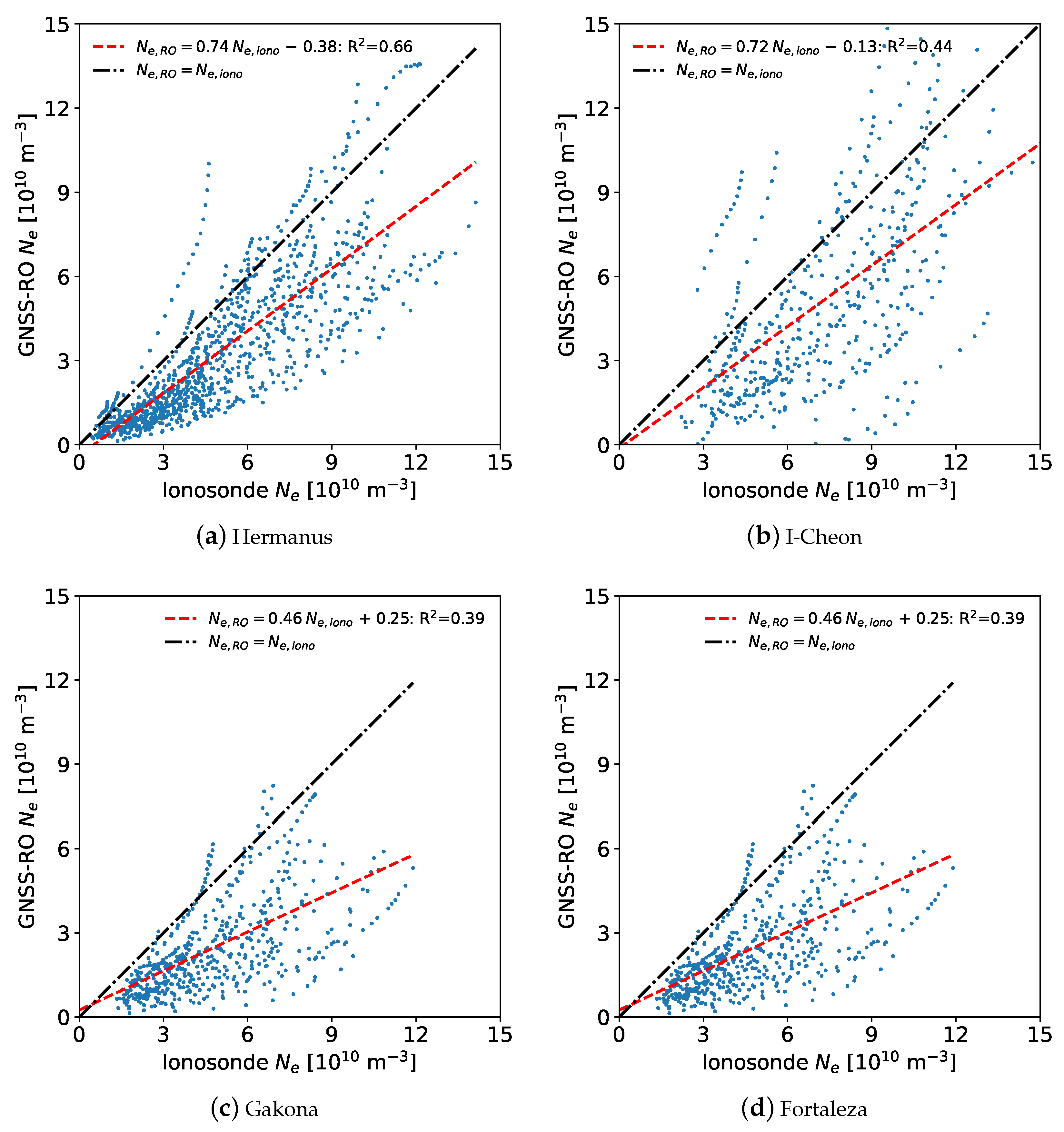
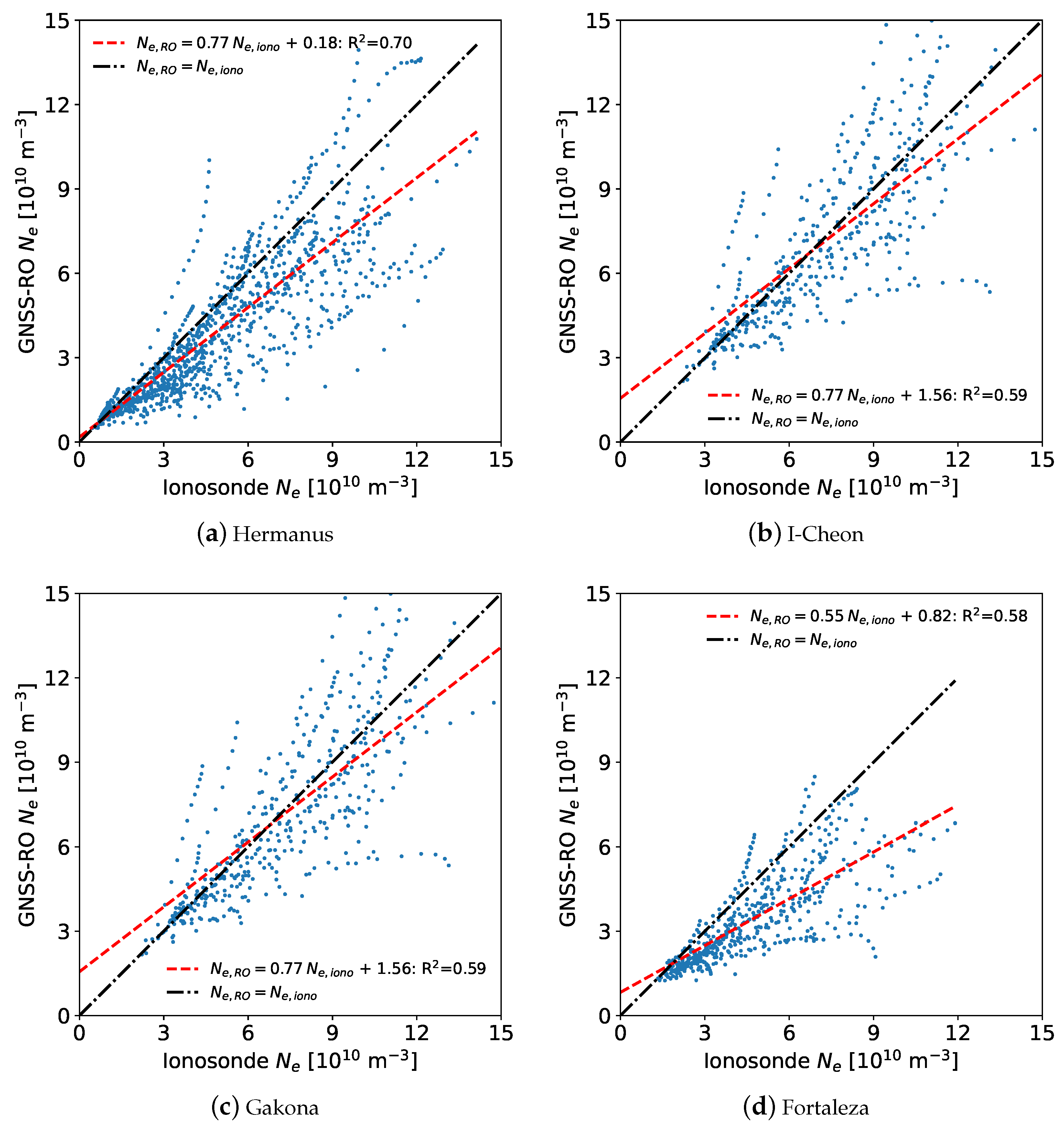
Electron density profiles were compared for both shifted and unshifted profiles using altitudes between fmin and hmE. Because the ionosonde profiles tend to be lower in altitude, the $N_e$ at any given altitude tends to be higher, which was evident for the unshifted profiles. For the shifted profiles, the $N_e$ values showed a stronger R² with a lower mean average error. The ionosonde $N_e$ was slightly larger on average than the GNSS-RO $N_e$.

Finally, virtual heights were calculated from the GNSS-RO profiles using a numerical ray tracer for comparison with direct ionosonde observations. Many of the GNSS-RO profiles showed reasonable agreement with the ionosonde observations near fmin, but there was an overall positive bias in the RO observations that could be due to low foE estimates or elevated hmE estimates. Interestingly, repeating the ray tracer comparison using ionosonde electron density profiles showed a negative altitude bias with respect to the direct observations, which may be due to the assumption of a quasi-parabolic layer shape. More research is required to fully understand this difference, however.

In conclusion, the general agreement between the bottom-up GNSS-RO profiles with both FIRI and ionosonde profiles indicates that this method is capable of providing global coverage of the D- and E-region ionosphere. The agreement between methods is strongest at lower altitudes near fmin with larger separation at higher altitudes near hmE, suggesting that the RO profiles are more trustworthy at lower altitudes and become less uncertain as altitude increases. These results reflect the optimal estimation design used for the bottom-up method that focuses on reducing negative electron density oscillations at the bottom of the profile. Further tuning of the optimal estimation weighting balance is the focus of an ongoing effort, which may help to reduce these uncertainties at higher altitudes. However, this technique may be used in its current form to provide global D- and E-region estimates for HF operations and analyses of global ionospheric dynamics at lower altitudes.

Due to the target fmin value and the time required to hand-scale ionograms, the dataset used for this research was limited. Ideally, this study would have included a seasonal comparison and morning-afternoon comparison at all sites, but this was not possible given the relatively small number of profiles. Future research should include a much larger dataset, which would require automatically scaled ionograms instead of the hand-scaled approach used here. Further, since this was the first in-depth comparison of the bottom-up method following the preliminary comparison performed in [23], the primary focus was on the quiet ionosphere. Therefore, future research should also include comparisons for the disturbed ionosphere, when sporadic-E is present.

References

1. Kelley, M.C. The Earth’s Ionosphere: Plasma Physics, and Electrodynamics; Academic Press: Cambridge, MA, USA, 2009. [Google Scholar]
2. Pisacane, V.L. The Space Environment and Its Effects on Space Systems; AIAA Press: Reston, VA, USA, 2008. [Google Scholar]
3. Fabrizio, G.A. High Frequency Over-the-Horizon Radar: Fundamental Principles, Signal Processing, and Practical Applications; McGraw-Hill Education: New York, NY, USA, 2013. [Google Scholar]
4. Kouba, D.; Chum, J. Ground-based measurements of ionospheric dynamics. J. Space Weather Space Clim. 2018, 8, A29. [Google Scholar] [CrossRef]
5. Titheridge, J.E. Ionogram Analysis with the Generalised Program POLAN; Report UAG; 93; National Oceanic and Atmospheric Administration: Washington, DC, USA, 1985.
6. Schunk, R.; Nagy, A. Ionospheres: Physics, Plasma Physics, and Chemistry; Cambridge University Press: Cambridge, UK, 2009. [Google Scholar]
7. Reinisch, B.; Bibl, K.; Kitrosser, D.F.; Sales, G.; Tang, J.; Zhang, Z.; Bullett, T.; Ralls, J. The Digisonde 256 ionospheric sounder. In World Ionosphere/Thermosphere Study, WITS Handbook; Liu, C.H., Ed.; SCOSTEP: Newton, MA, USA, 1989; Volume 2. [Google Scholar]
8. Lowell GIRO Data Center. Global Ionosphere Radio Observatory. 2022. Available online: http://giro.uml.edu/ (accessed on 1 December 2022).
9. Thom, M. Radio Occultation in Less than 500 Words. 2023. Available online: https://spire.com/blog/maritime/radio-occultation-in-less-than-500-words/ (accessed on 1 July 2023).
10. Schreiner, W.; Weiss, J.; Anthes, R.; Braun, J.; Chu, V.; Fong, J.; Hunt, D.; Kuo, Y.H.; Meehan, T.; Serafino, W.; et al. COSMIC-2 radio occultation constellation: First results. Geophys. Res. Lett. 2020, 47, e2019GL086841. [Google Scholar] [CrossRef]
11. Hajj, G.A.; Ibañez-Meier, R.; Kursinski, E.R.; Romans, L.J. Imaging the ionosphere with the Global Positioning System. Int. J. Imaging Syst. Technol. 1994, 5, 174–187. [Google Scholar] [CrossRef]
12. Hajj, G.A.; Romans, L.J. Ionospheric electron density profiles obtained with the Global Positioning System: Results from the GPS/MET experiment. Radio Sci. 1998, 33, 175–190. [Google Scholar] [CrossRef]
13. Schreiner, W.S.; Sokolovskiy, S.V.; Rocken, C.; Hunt, D.C. Analysis and validation of GPS/MET radio occultation data in the ionosphere. Radio Sci. 1999, 34, 949–966. [Google Scholar] [CrossRef]
14. Syndergaard, S. A new algorithm for retrieving GPS radio occultation total electron content. Geophys. Res. Lett. 2002, 29, 55-1–55-4. [Google Scholar] [CrossRef]
15. Nicolls, M.J.; Rodrigues, F.S.; Bust, G.S.; Chau, J.L. Estimating E region density profiles from radio occultation measurements assisted by IDA4D. J. Geophys. Res. Space Phys. 2009, 114, A10316. [Google Scholar] [CrossRef]
16. Yue, X.; Schreiner, W.S.; Kuo, Y.H. Evaluating the effect of the global ionospheric map on aiding retrieval of radio occultation electron density profiles. GPS Solut. 2013, 17, 327–335. [Google Scholar] [CrossRef]
17. Yue, X.; Schreiner, W.S.; Lei, J.; Sokolovskiy, S.V.; Rocken, C.; Hunt, D.C.; Kuo, Y.H. Error analysis of Abel retrieved electron density profiles from radio occultation measurements. Ann. Geophys. 2010, 28, 217–222. [Google Scholar] [CrossRef]
18. Wu, K.H.; Su, C.L.; Chu, Y.H. Improvement of GPS radio occultation retrieval error of E region electron density: COSMIC measurement and IRI model simulation. J. Geophys. Res. Space Phys. 2015, 120, 2299–2315. [Google Scholar] [CrossRef]
19. Pedatella, N.M.; Yue, X.; Schreiner, W.S. An improved inversion for FORMOSAT-3/COSMIC ionosphere electron density profiles. J. Geophys. Res. Space Phys. 2015, 120, 8942–8953. [Google Scholar] [CrossRef]
20. Tulasi Ram, S.; Su, S.Y.; Tsai, L.C.; Liu, C.H. A self-contained GIM-aided Abel retrieval method to improve GNSS-Radio Occultation retrieved electron density profiles. GPS Solut. 2016, 20, 825–836. [Google Scholar] [CrossRef]
21. Gowtam, V.S.; Ram, S.T.; Ankita, M. An aided Abel inversion technique assisted by artificial neural network-based background ionospheric model for near real-time correction of FORMOSAT-7/COSMIC-2 data. Adv. Space Res. 2021, 68, 2865–2875. [Google Scholar] [CrossRef]
22. Wu, D.L. New global electron density observations from GPS-RO in the D- and E-Region ionosphere. J. Atmos. Sol.-Terr. Phys. 2018, 171, 36–59. [Google Scholar] [CrossRef]
23. Wu, D.L.; Emmons, D.J.; Swarnalingam, N. Global GNSS-RO electron density in the lower ionosphere. Remote Sens. 2022, 14, 1577. [Google Scholar] [CrossRef]
24. University Cooperation for Atmospheric Research. COSMIC Data Analysis and Archive Center. 2022. Available online: https://cdaac-www.cosmic.ucar.edu/ (accessed on 1 December 2022).
25. Rodgers, C.D. Inverse Methods for Atmospheric Sounding: Theory and Practice; World Scientific: Singapore, 2000; Volume 2. [Google Scholar]
26. Bilitza, D. IRI the international standard for the ionosphere. Adv. Radio Sci. 2018, 16, 1–11. [Google Scholar] [CrossRef]
27. Rishbeth, H.; Garriott, O.K. Introduction to ionospheric physics. IEEE Trans. Image Process. 1969, 1, 131. [Google Scholar]
28. Huang, X.; Reinisch, B.W. Automatic calculation of electron density profiles from digital ionograms: 2. True height inversion of topside ionograms with the profile-fitting method. Radio Sci. 1982, 17, 837–844. [Google Scholar] [CrossRef]
29. Reinisch, B.W.; Xueqin, H. Automatic calculation of electron density profiles from digital ionograms: 3. Processing of bottomside ionograms. Radio Sci. 1983, 18, 477–492. [Google Scholar] [CrossRef]
30. Galkin, I.; Reinisch, B.W.; Huang, X.; Khmyrov, G.M. Confidence score of ARTIST-5 ionogram autoscaling. Ionosonde Netw. Advis. Group (INAG) Bull. 2013, 73, 1–7. [Google Scholar]
31. Themens, D.R.; Reid, B.; Elvidge, S. ARTIST ionogram autoscaling confidence scores: Best practices. URSI Radio Sci. Lett. 2022, 4, 1–5. [Google Scholar]
32. Galkin, I.A.; Reinisch, B.W. The new ARTIST 5 for all digisondes. Ionosonde Netw. Advis. Group Bull. 2008, 69, 1–8. [Google Scholar]
33. Titheridge, J. Ionogram analysis: Least squares fitting of a Chapman-layer peak. Radio Sci. 1985, 20, 247–256. [Google Scholar] [CrossRef]
34. Friedrich, M.; Torkar, K. FIRI: A semiempirical model of the lower ionosphere. J. Geophys. Res. Space Phys. 2001, 106, 21409–21418. [Google Scholar] [CrossRef]
35. Friedrich, M.; Pock, C.; Torkar, K. FIRI-2018, an updated empirical model of the lower ionosphere. J. Geophys. Res. Space Phys. 2018, 123, 6737–6751. [Google Scholar] [CrossRef]
36. Chau, J.L.; Woodman, R.F. D and E region incoherent scatter radar density measurements over Jicamarca. J. Geophys. Res. Space Phys. 2005, 110, A12314. [Google Scholar] [CrossRef]
37. Swarnalingam, N.; Wu, D.; Themens, D. Comparison and evaluation of a bottom-up GPS-RO electron density retrieval for D and E regions using radar observations and models. J. Atmos. Sol.-Terr. Phys. 2020, 207, 105333. [Google Scholar] [CrossRef]
38. Goddard Space Flight Center. OMNIWeb Data Explorer. 2022. Available online: https://omniweb.gsfc.nasa.gov/form/dx1.html (accessed on 1 December 2022).
39. Jones, R.; Stephenson, J. A Versatile Three-Dimensional Ray Tracing Computer Program for Radio Waves in the Ionosphere; U.S. Department of Commerce, Office of Telecommunications: Washington, DC, USA, 1975.
40. McNamara, L.F.; Cooke, D.L.; Valladares, C.E.; Reinisch, B.W. Comparison of CHAMP and Digisonde plasma frequencies at Jicamarca, Peru. Radio Sci. 2007, 42, 1–14. [Google Scholar] [CrossRef]
41. Huang, X.; Reinisch, B. Vertical electron density profiles from the Digisonde network. Adv. Space Res. 1996, 18, 121–129. [Google Scholar] [CrossRef]
42. McNamara, L.F. Model starting heights for N(h) analyses of ionograms. J. Atmos. Terr. Phys. 1979, 41, 543–547. [Google Scholar] [CrossRef]
43. Titheridge, J. Starting models for the real height analysis of ionograms. J. Atmos. Terr. Phys. 1986, 48, 435–446. [Google Scholar] [CrossRef]
44. Liu, J.Y.; Lin, C.Y.; Lin, C.H.; Tsai, H.F.; Solomon, S.C.; Sun, Y.Y.; Lee, I.T.; Schreiner, W.S.; Kuo, Y.H. Artificial plasma cave in the low-latitude ionosphere results from the radio occultation inversion of the FORMOSAT-3/COSMIC. J. Geophys. Res. Space Phys. 2010, 115, A07319. [Google Scholar] [CrossRef]
45. Wu, D.L.; Swarnalingam, N.; Salinas, C.C.J.H.; Emmons, D.J.; Summers, T.C.; Gardiner-Garden, R. Optimal Estimation Inversion of Ionospheric Electron Density from GNSS-POD Limb Measurements: Part I-Algorithm and Morphology. Remote Sens. 2023, 15, 3245. [Google Scholar] [CrossRef]
46. Leitinger, R.; Ladreiter, H.P.; Kirchengast, G. Ionosphere tomography with data from satellite reception of Global Navigation Satellite System signals and ground reception of Navy Navigation Satellite System signals. Radio Sci. 1997, 32, 1657–1669. [Google Scholar] [CrossRef]
47. Nicolls, M.J.; Rodrigues, F.S.; Bust, G.S. Global observations of E region plasma density morphology and variability. J. Geophys. Res. Space Phys. 2012, 117, A01305. [Google Scholar] [CrossRef]
48. McNamara, L.F. The Ionosphere: Communications, Surveillance, and Direction Finding; Krieger Publishing Company: Malabar, FL, USA, 1991. [Google Scholar]
Figure 1. GNSS-RO uncertainties calculated using the optimal estimation method on 200 profiles from 1 Jan 2023. ‘Eden’ is the electron density (black) and ‘Unc’ is the altitude dependent uncertainty (red) with units of 10 5 cm−3 (10 11 m−3). ‘Index’ in the lower-right figure corresponds to the phase standard deviation between 50–55 km (black), and ‘Chisq_80km’ is a quality index used to estimate ionospheric impacts on the neutral atmosphere (red).
Remotesensing 15 04363 g001
Figure 2. Local solar time histograms for each site. The hand-scaling process naturally filtered out nighttime profiles, and the wide range at Gakona is due to the length of summer days at high latitudes.
Remotesensing 15 04363 g002
Figure 3. Individual electron profile comparison examples. The GNSS-RO and ionosonde real height profiles have a similar shape in the E-region, but are separated in altitude. The CDAAC descriptors displayed here are (a) atmPhs_C004.2010.273.06.22.G17_2013.3520, (b) atmPhs_C002.2013.054.04.43.G22_2013.3520, (c) atmPhs_C005.2011.174.04.34.G20_2013.3520, and (d) atmPhs_C2E2.2020.262.09.28.R20_0001.0001.
Remotesensing 15 04363 g003
Figure 4. Shifted individual electron density profile comparison examples. These are the same profiles used in Figure 3 which show close agreement in the bottomside E-region after the profiles are shifted in altitude to match at fmin.
Remotesensing 15 04363 g004
Figure 5. Average unshifted and shifted EDPs at Hermanus for GNSS-RO and ionosonde measurements showing general agreement between fmin and hmE. The average density was calculated in 1 km increments and is shown with standard deviation uncertainties. Error bars are used for ionosondes and shading is used for GNSS-RO.
Remotesensing 15 04363 g005
Figure 6. Average unshifted and shifted EDPs at I-Cheon for GNSS-RO and ionosonde measurements showing agreement near fmin and a continual growth with altitude for the GNSS-RO observations that is not observed for the ionosondes.
Remotesensing 15 04363 g006
Figure 7. Average unshifted and shifted EDPs at Gakona for GNSS-RO and ionosonde measurements showing similar trends but with the ionosonde densities slightly higher.
Remotesensing 15 04363 g007
Figure 8. Average unshifted and shifted EDPs at Fortaleza for GNSS-RO and ionosonde measurements showing agreement near fmin and a continual growth with altitude for the GNSS-RO observations that is not observed for the ionosondes.
Remotesensing 15 04363 g008
Figure 9. Average EDPs for GNSS-RO measurements and FIRI predictions for each site showing general agreement in the D- to E-transition region. The average density was calculated in 1 km increments and is shown with standard deviation uncertainties, shown by shading for both profiles. Note that the electron density scale varies between sites.
Remotesensing 15 04363 g009
Figure 10. A comparison of GNSS-RO and ionogram foE measurements. The black line is the 1:1 line, and the red line is the linear fit. Most of the slopes are near one, with the exception of I-Cheon which contained the fewest RO profiles with a clear E-region peak.
Remotesensing 15 04363 g010
Figure 11. GNSS-RO—ionogram foE histograms and CDFs. The red line is the CDF, the blue boxes are relative frequency, the solid black line is the mean, and the dashed black lines are ±1 standard deviation. Most of the sites show an average difference around zero MHz except for Gakona which shows a negative bias.
Remotesensing 15 04363 g011
Figure 12. A comparison of GNSS-RO and ionogram hmE measurements. The black line is the 1:1 line, and the red line is the linear fit. GNSS-RO hmE show less variation than the ionosonde hmE values. Most sites show a positive bias due to the limited variation in GNSS-RO hmE altitudes.
Remotesensing 15 04363 g012
Figure 13. GNSS-RO—ionogram hmE histograms and CDFs. The red line is the CDF, the blue boxes are relative frequency, the solid black line is the mean, and the dashed black lines are ±1 standard deviation.
Remotesensing 15 04363 g013
Figure 14. Unshifted GNSS-RO and ionosonde N e measurements for altitudes between fmin and hmE which show an under-prediction for the GNSS-RO values due to an altitude bias between the two sets of measurements. The black line is the 1:1 line, and the linear fit is in red.
Remotesensing 15 04363 g014
Figure 15. Shifted GNSS-RO and ionosonde N e measurements for altitudes between fmin and hmE showing general agreement for most sites. The black line is the 1:1 line, and the linear fit is in red.
Remotesensing 15 04363 g015
Figure 16. Shifted GNSS-RO−ionosonde N e difference histograms showing larger differences at higher altitudes. The color bar represents the number of measurements in each bin. A total of 400 bins were used ( 20 × 20 ) and the color bar represents the number of measurements in each bin.
Remotesensing 15 04363 g016
Figure 17. Virtual height profiles calculated from GNSS-RO using a numerical ray tracer along with the direct ionosonde measurements showing general agreement in the trends. These virtual height profiles correspond to the electron density profiles displayed in Figure 3 and Figure 4.
Remotesensing 15 04363 g017
Figure 18. A comparison of GNSS-RO and ionosonde virtual heights with the RO virtual heights calculated using a numerical ray tracer. The midlatitude sites show a clustering near the 1:1 line near fmin altitudes and all sites show a positive bias for the lower altitudes.
Remotesensing 15 04363 g018
Figure 19. GNSS-RO—ionosonde virtual height difference histograms and CDFs which show a positive bias for all sites except Fortaleza. The Frequency on the right corresponds to the number of datapoints within each bin.
Remotesensing 15 04363 g019
Figure 20. Virtual heights calculated from ionosonde EDPs compared with ionosonde virtual height measurements. Interestingly, there is a negative bias for the virtual heights calculated from the profiles using a ray tracer.
Remotesensing 15 04363 g020
Figure 21. Calculated d z / d f p for the shifted GNSS-RO and ionosonde profiles which show elevated ionosonde derivatives at higher altitudes near hmE.
Remotesensing 15 04363 g021