
Evaluation and Projection of Precipitation in CMIP6 Models over the Qilian Mountains, China


Abstract
:
1. Introduction
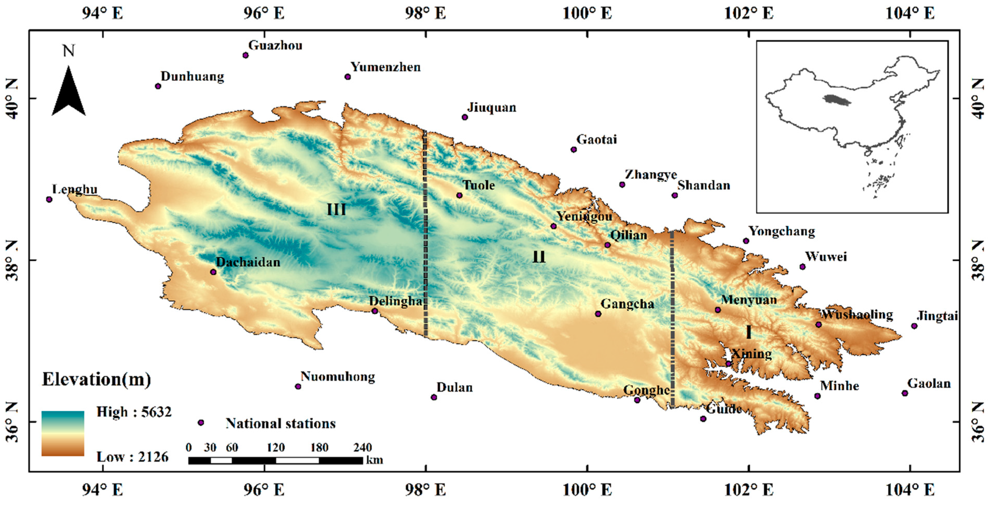
2. Study Area
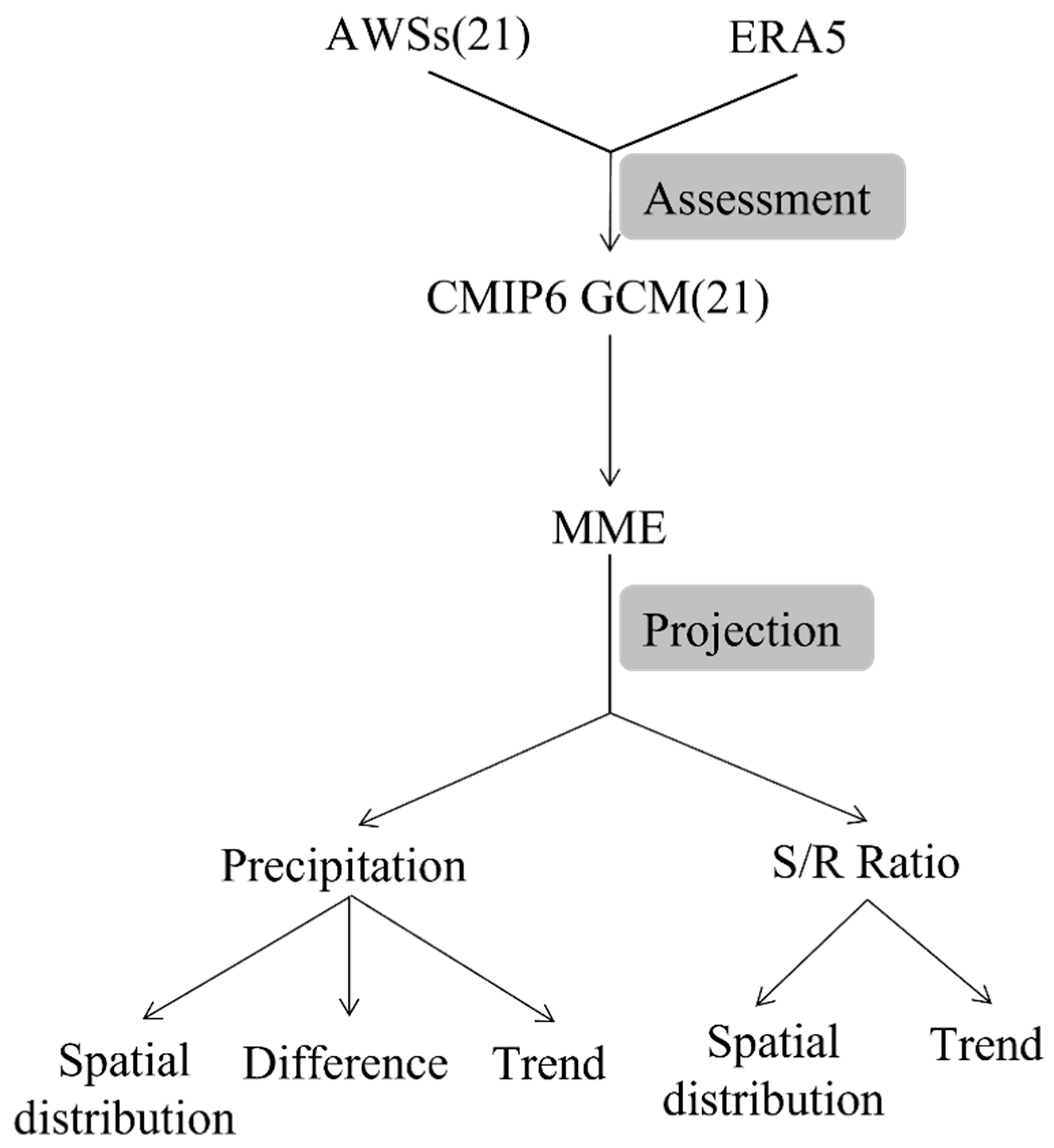
3. Data and Methods
3.1. Precipitation Data
3.2. Methods
4. Results
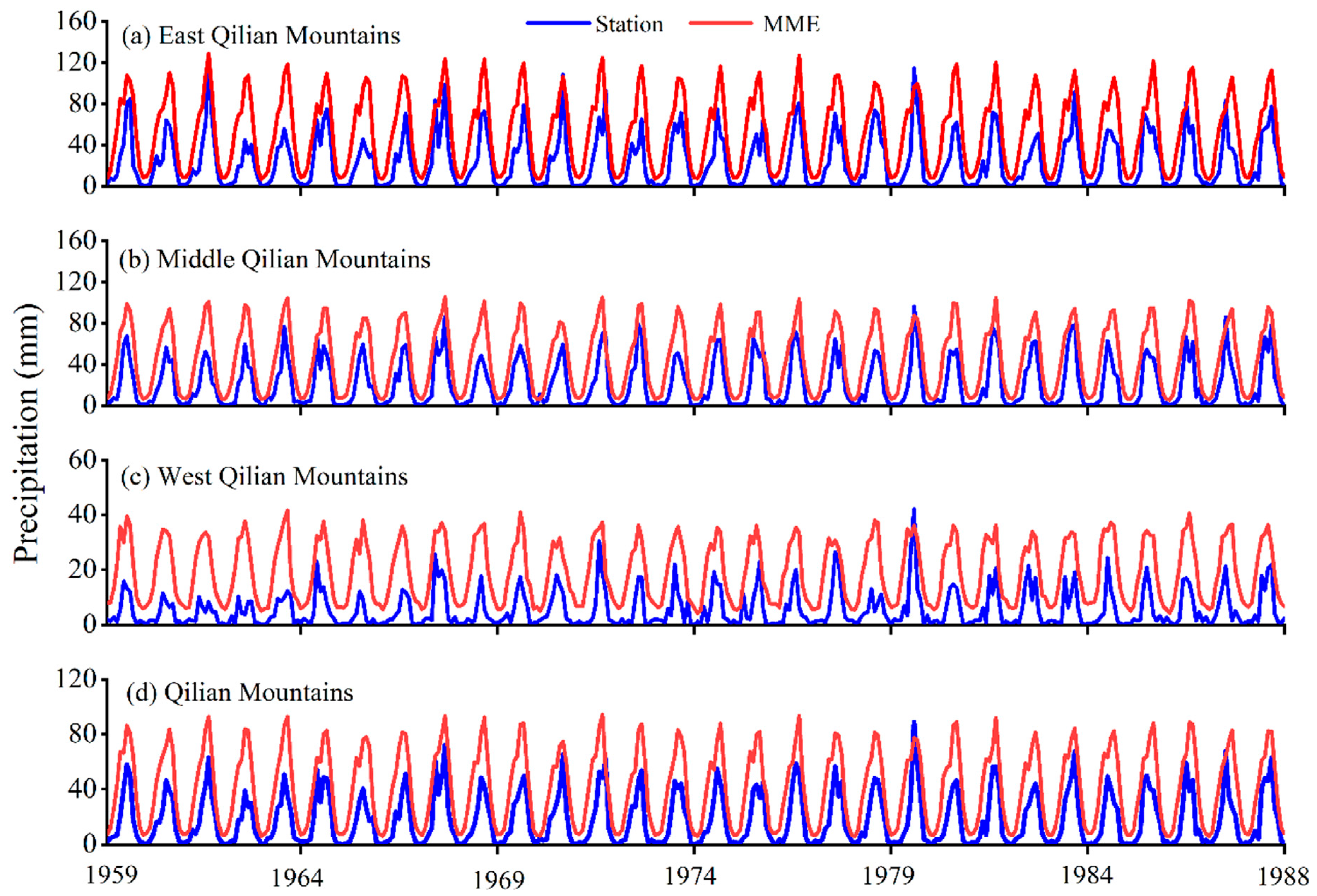
4.1. CMIP6 Model Performance
4.2. Projections of Changes in Precipitation in the 21st Century
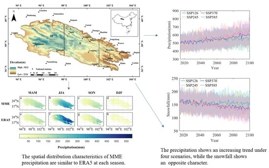
4.2.1. Spatial Distribution of Precipitation
4.2.2. Precipitation Difference
4.2.3. Precipitation Trends
4.3. Changes in the Snow-to-Rain Ratio in the 21st Century
5. Discussion
5.1. Factors Affecting Precipitation Changes
5.2. The Biases and Uncertainty of the Models
6. Conclusions
- (1)
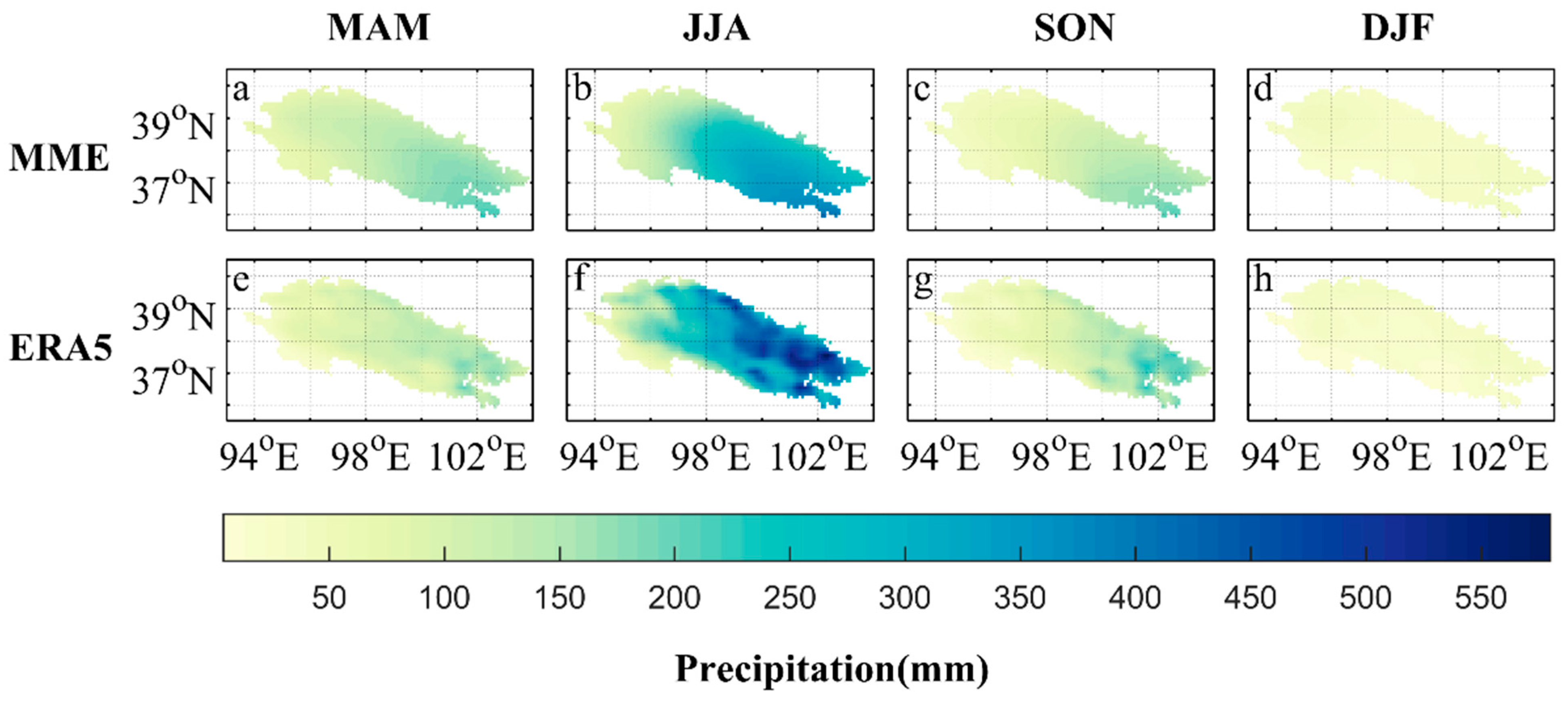
- The CMIP6 models exhibited reasonable simulation ability for the spatial distribution of annual precipitation in the QMs. In the historical period, MME was concentrated between 476.99 and 546.96 mm, ERA5 was concentrated between 406.11 and 587.07 mm, and the simulation results were the best in the central region, with an error between −100 and 100 mm. Simulations were low in the north and northeast, and they were high in the south and southeast. The climatic tendency rate of MME was −2.01 mm·10a−1, which was slightly lower than that of ERA5 (2.82 mm·10a−1). It can be seen that MME and ERA5 have a high degree of agreement overall.
- (2)
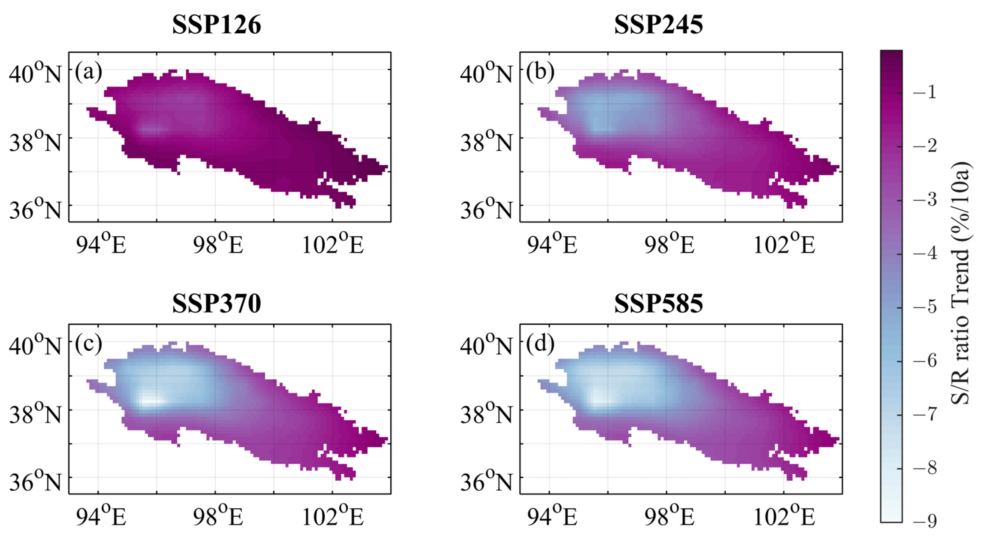
- Precipitation and rainfall showed a decreasing trend from southeast to northwest; the more severe the emissions scenario, the more significant the observed decreasing pattern. The trend in snowfall and the snow-to-rain ratio were reversed, showing an increasing trend from southeast to northwest. As the emissions scenario (concentrations of CO2, CH4, N2O and other gases’) became more severe, the increase became more significant.
- (3)
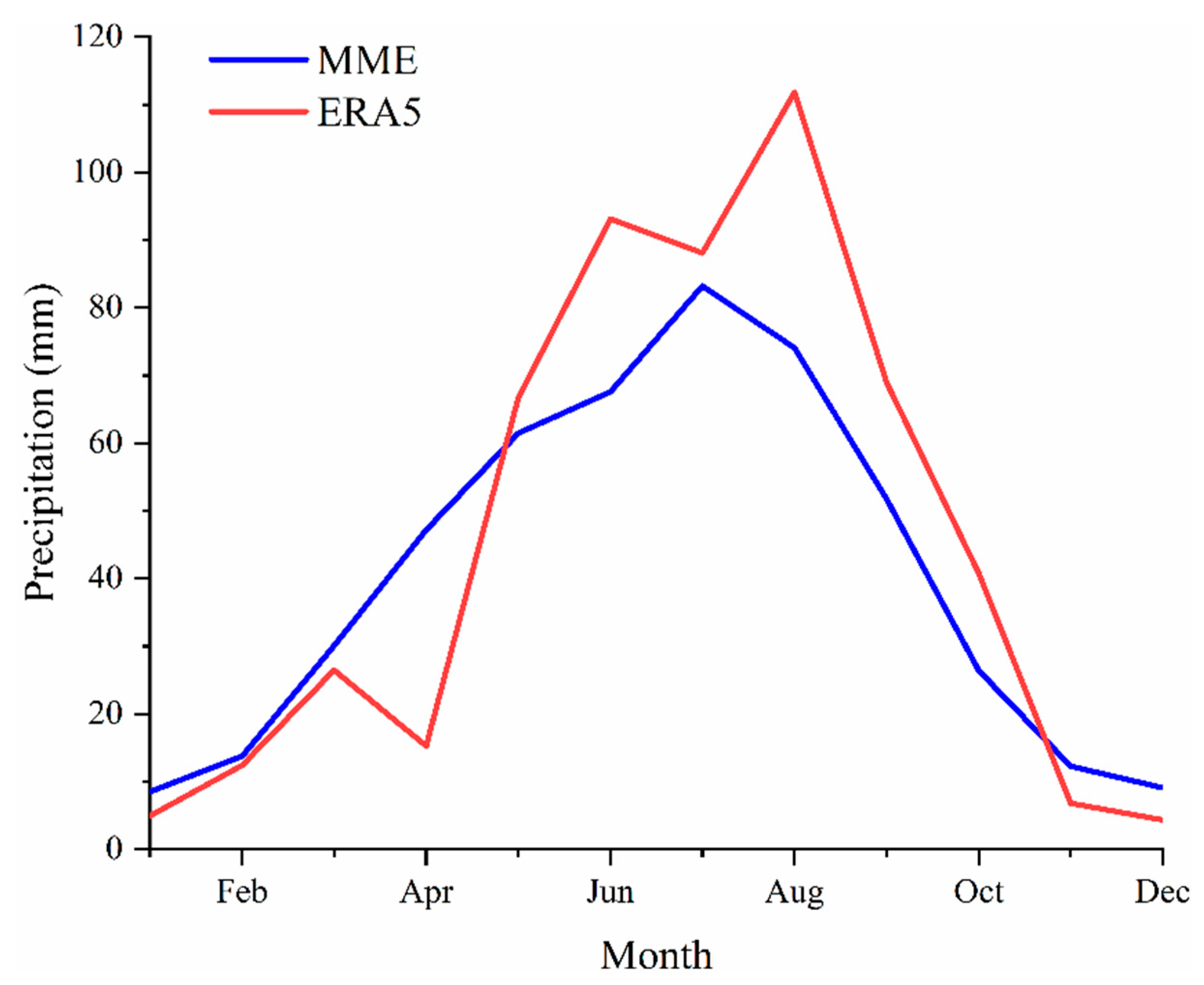
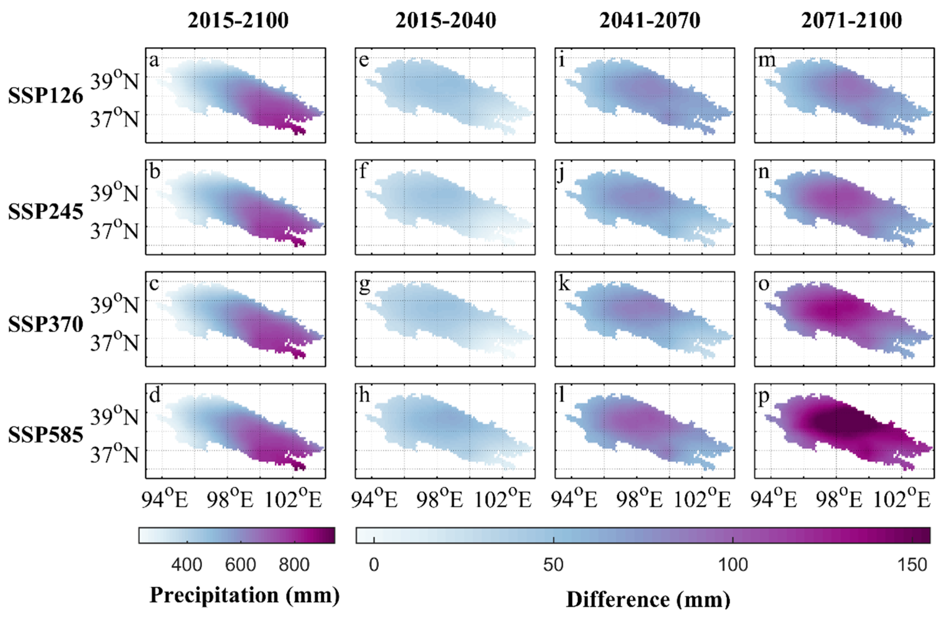
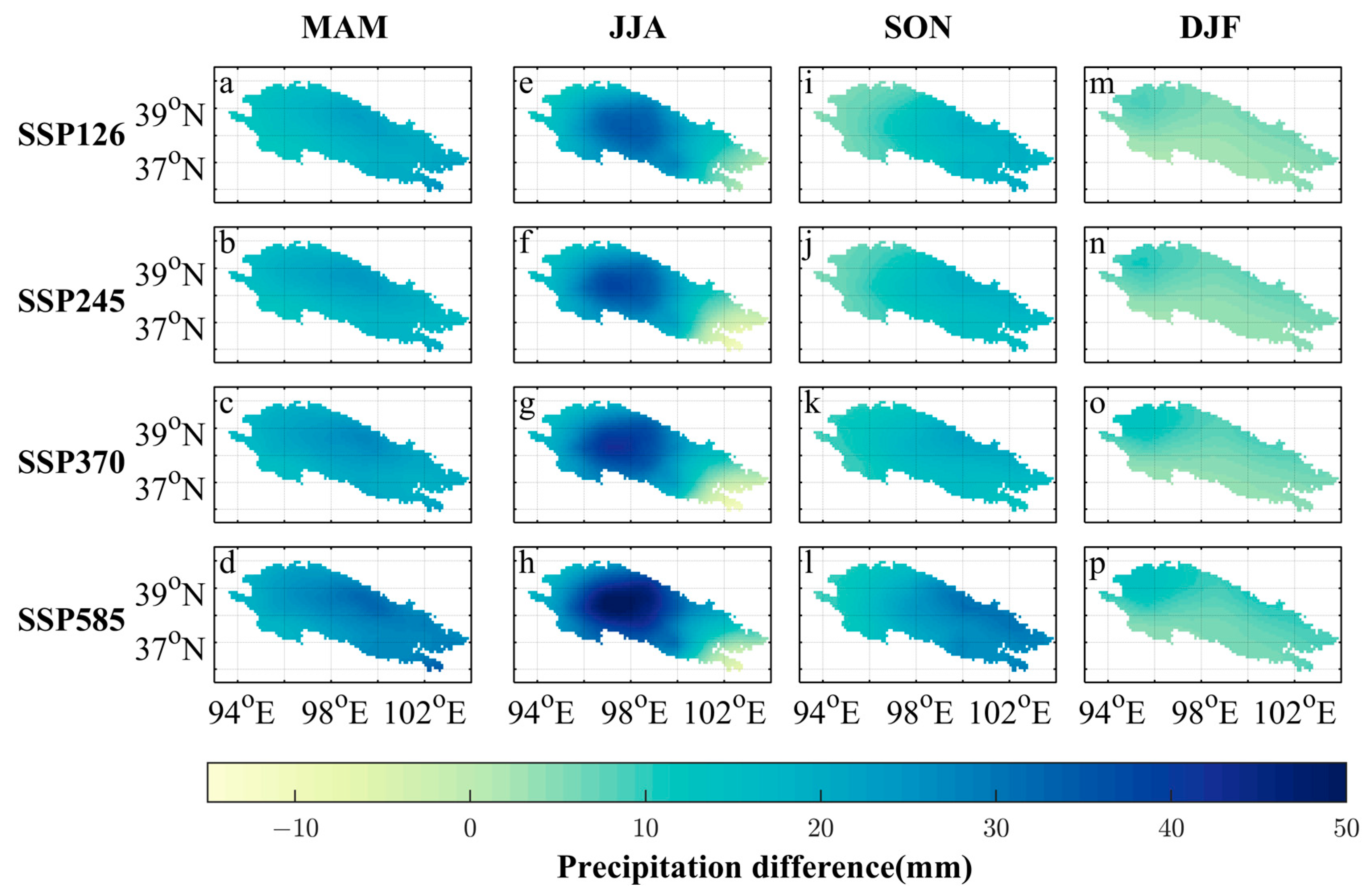
- Regarding the time scale, the precipitation in the historical period (1959–1988) fluctuated and rose. From 1959 to 1988, the average seasonal precipitation of MME in spring, summer, autumn, and winter was 130.07, 224.62, 95.96, and 29.07 mm, respectively, and that of ERA5 was 98.57, 280.77, 96.85, and 22.64 mm, respectively. From 2015 to 2100, the difference between the future and historical period from MME, which was especially pronounced in summer, was 21.52, 20.48, 23.00, and 29.24 mm in spring, summer, autumn, and winter, respectively. Meanwhile, the climate tendency rates of average precipitation from MME in spring, summer, autumn, and winter were 5.73, 9.15, 12.23 and 16.14 mm·10a−1, respectively. The flood season in the QMs is July and August, and precipitation could reach more than 80 mm. Rainfall rates also rose, while the snowfall and snow-to-rain ratio showed a downward trend; the higher emissions scenario (concentrations of CO2, CH4, N2O, and other gases) resulted in a more significant reduction.
- (4)
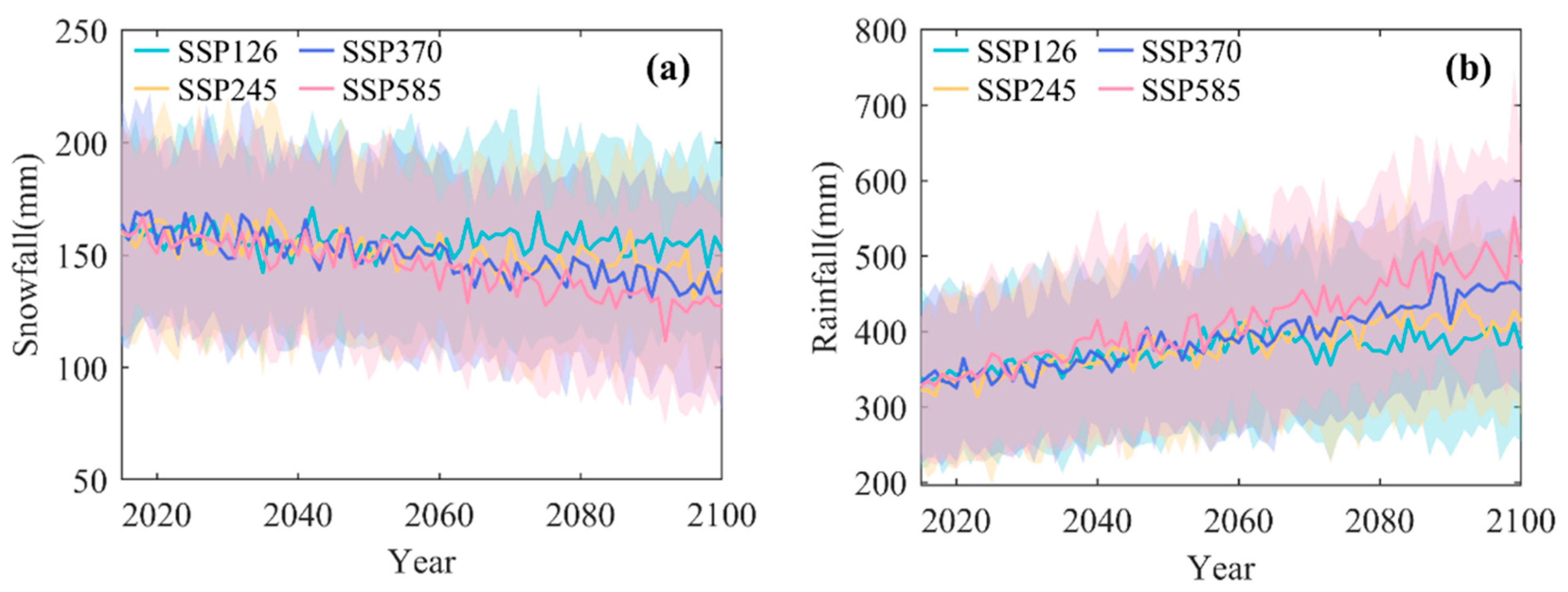
- During the period 2015–2100, the snowfall ratio ranged from 0.1 to 1.1. The annual snowfall showed a decreasing trend, the climatic tendency rate ranged from −10 to 0.1 mm·10a−1, and the rainfall always showed an increasing trend (0–30 mm.10a−1), with both passing the significance test (p < 0.05). The snow-to-rain ratio was the highest in winter in the four scenarios, with values of 16.77, 17.14, 15.82, and 15.26, because snow is mainly concentrated in winter.
Supplementary Materials
Author Contributions
Funding
Data Availability Statement
Acknowledgments
Conflicts of Interest
References
- Chen, R.; Han, C.; Wang, L.; Zhao, Y.; Song, Y.; Yang, Y.; Liu, J.; Liu, Z.; Wang, X.; Guo, S.; et al. Surface precipitation and high mountain areas in Qilian Mountains in 2019–2020 Precipitation monitoring significance. J. Glaciol. Geocryol. 2023, 45, 676–687. [Google Scholar]
- Yao, T.; Wang, Y.; Liu, S.; Pu, J.; Shen, Y.; Lu, A. Recent glacial retreat in High Asia in China and its impact on water resource in Northwest China. Sci. China Ser. D Earth Sci. 2004, 47, 1065–1075. [Google Scholar] [CrossRef]
- Zhao, C.; Ding, Y.; Yao, S. The variation of precipitation and rain days for different intensity classes during the rainy season in the Qilian Mountains, Northwest China. Theor. Appl. Climatol. 2021, 144, 163–178. [Google Scholar] [CrossRef]
- Yang, B.; Qin, C.; Wang, J.; He, M.; Melvin, T.M.; Osborn, T.J.; Briffa, K.R. A 3500-year tree-ring record of annual precipitation on the northeastern Tibetan Plateau. Proc. Natl. Acad. Sci. USA 2014, 111, 2903–2908. [Google Scholar] [CrossRef]
- Ji, F.; Wu, Z.H.; Huang, J.P.; Chassignet, E.P. Evolution of land surface air temperature trend. Nat. Clim. Chang. 2014, 4, 462–466. [Google Scholar] [CrossRef]
- Han, L.J.; Bai, A.J.; Pu, X.M. Climate change characteristics estimation in the Qilian Mountains based on CMIP6. Plateaumeteorology 2022, 41, 864–875. [Google Scholar]
- Qin, D.; Zhen, C.; Yong, L.; Yihui, D.; Dai, X.S.; Jia, W.R. The latest understanding of climate change science. Prog. Clim. Chang. Res. 2007, 3, 63–73. [Google Scholar]
- Li, Y.Z.; Qin, X.; Liu, Y.S.; Jin, Z.Z.; Liu, J.; Wang, L.H.; Chen, J.Z. Evaluation of Long-Term and High-Resolution Gridded Precipitation and Temperature Products in the Qilian Mountains, Qinghai-Tibet Plateau. Front. Environ. Sci. 2022, 10, 906821. [Google Scholar] [CrossRef]
- Shi, Y.; Shen, Y. A preliminary study on the signals, impacts and prospects of the transition of climate from warm dry to warm and humid climate in northwest China. Sci. Technol. Rev. 2003, 23, 54–57. [Google Scholar] [CrossRef]
- Li, D.L.; Xie, J.N.; Wang, W. Study on summer precipitation characteristics and anomalies in northwest China. Atmos. Sci. 1997, 21, 76–85. [Google Scholar] [CrossRef]
- Ma, Z.G. The evolution of dry and wet in northern China and its possible connection with regional warming. Chin. J. Geophys. 2005, 48, 1011–1018. [Google Scholar] [CrossRef]
- Qin, D.H.; Yao, T.D.; Ding, Y.J.; Ren, J.W. The establishment of the cryosphere scientific system and its significance. Bull. Chin. Acad. Sci. 2020, 35, 394–406. [Google Scholar] [CrossRef]
- Wang, L.; Ren, S.C.; Yao, X.S. Research review on calculation methods and influential factors on areal precipitation of alpine mountains. Plateau Meteorol. 2017, 36, 1546–1556. [Google Scholar]
- Zhao, T.; Fu, C.; Ke, Z.; Guo, W. Global Atmosphere Reanalysis Datasets: Current Status and Recent Advances. Adv. Earth Sci. 2010, 25, 241. [Google Scholar]
- Chen, L.; Frauenfeld, O.W. A comprehensive evaluation of precipitation simulations over China based on CMIP5 multimodel ensemble projections. J. Geophys. Res. Atmos. 2014, 119, 5767–5786. [Google Scholar] [CrossRef]
- Fan, X.W.; Duan, Q.Y.; Shen, C.W.; Wu, Y.; Xing, C. Global surface air temperatures in CMIP6: Historical performance and future changes. Environ. Res. Lett. 2020, 15, 14. [Google Scholar] [CrossRef]
- Wei, C.; Da, B.J.; Xiao, X.W. Evaluation and Projection of CMIP6 Models for Climate over the Qinghai-Xizang (Tibetan) Plateau. Plateau Meteorol. 2021, 40, 1455–1469. [Google Scholar]
- Qin, H.; Da, B.J.; Guang, Z.F. Evaluation of CMIP5 models over the Qinghai-Tibetan Plateau. Chin. J. Atmos. Sci. 2014, 38, 924–938. [Google Scholar]
- Zhen, C.L.; Zhi, G.W.; Shi, H.L.; Yan, H.G.; Bo, H.; Suo, L. Verifications of surface air temperature and precipitation from CMIP5 Model in Northern Hemisphere and Qinghai Xizang Plateau. Plateau Meteorol. 2013, 32, 921–928. [Google Scholar]
- Jing, W.; Bao, J.W.; Yan, F.Y.; Yan, C.; Lin, C.; Jian, C.Y.; Xin, W.L. Comparing simulated temperature and precipitation of CMIP3 and CMIP5 in arid areas of Northwest China. Clim. Chang. Res. 2017, 13, 198–212. [Google Scholar]
- Stocker, T. Climate Change 2013: The Physical Science Basis: Working Group I Contribution to the Fifth Assessment Report of the Intergovernmental Panel on Climate Change; Cambridge University Press: Cambridge, UK, 2014. [Google Scholar]
- Ying, X.; Chong, H.X. Preliminary assessment of simulations of climate changes over China by CMIP5 multi-models. Atmos. Ocean. Sci. Lett. 2012, 5, 489–494. [Google Scholar] [CrossRef]
- Su, F.; Duan, X.; Chen, D.; Hao, Z.; Cuo, L. Evaluation of the Global Climate Models in the CMIP5 over the Tibetan Plateau. J. Clim. 2013, 26, 3187–3208. [Google Scholar] [CrossRef]
- Moss, R.H.; Edmonds, J.A.; Hibbard, K.A.; Manning, M.R.; Rose, S.K.; van Vuuren, D.P.; Carter, T.R.; Emori, S.; Kainuma, M.; Kram, T.; et al. The next generation of scenarios for climate change research and assessment. Nature 2010, 463, 747–756. [Google Scholar] [CrossRef] [PubMed]
- Tian, J.Z.; Wen, X.Z.; Xiao, L.C.; Li, X.Z.; Li, W.Z.; Wen, M.M. The nearterm, mid-term and long-term projections of temperature and precipitation changes over the Tibetan Plateau and the sources of uncertainties. J. Meteorol. Sci. 2020, 40, 697–710. [Google Scholar]
- Zhou, T.J.; Zou, L.W.; Chen, X.L. Review of the Sixth International Coupling Model Comparison Program (CMIP6). Prog. Clim. Chang. Res. 2019, 15, 445–456. [Google Scholar]
- Gusain, A.; Ghosh, S.; Karmakar, S. Added value of CMIP6 over CMIP5 models in simulating Indian summer monsoon rainfall. Atmos. Res. 2020, 232, 8. [Google Scholar] [CrossRef]
- Rivera, J.A.; Arnould, G. Evaluation of the ability of CMIP6 models to simulate precipitation over Southwestern South America: Climatic features and long-term trends (1901–2014). Atmos. Res. 2020, 241, 15. [Google Scholar] [CrossRef]
- O’Neill, B.C.; Tebaldi, C.; van Vuuren, D.P.; Eyring, V.; Friedlingstein, P.; Hurtt, G.; Knutti, R.; Kriegler, E.; Lamarque, J.F.; Lowe, J.; et al. The Scenario Model Intercomparison Project (ScenarioMIP) for CMIP6. Geosci. Model Dev. 2016, 9, 3461–3482. [Google Scholar] [CrossRef]
- Ullah, I.; Saleem, F.; Iyakaremye, V.; Yin, J.; Ma, X.; Syed, S.; Hina, S.; Asfaw, T.G.; Omer, A. Projected Changes in Socioeconomic Exposure to Heatwaves in South Asia under Changing Climate. Earth’s Future 2022, 10, e2021EF002240. [Google Scholar] [CrossRef]
- Wu, J.; Shi, Y.; Xu, Y. Evaluation and Projection of Surface Wind Speed Over China Based on CMIP6 GCMs. J. Geophys. Res. Atmos. 2020, 125, e2020JD033611. [Google Scholar] [CrossRef]
- Zhao, S.; Yu, Y.; Lin, P.; Liu, H.; He, B.; Bao, Q.; Guo, Y.; Hua, L.; Chen, K.; Wang, X. Datasets for the CMIP6 Scenario Model Intercomparison Project (ScenarioMIP) Simulations with the Coupled Model CAS FGOALS-f3-L. Adv. Atmos. Sci. 2021, 38, 329–339. [Google Scholar] [CrossRef]
- Chen, R.S.; Han, C.T.; Liu, J.F.; Yang, Y.; Liu, Z.W.; Wang, L.; Kang, E.S. Maximum precipitation altitude on the northern flank of the Qilian Mountains, northwest China. Hydrol. Res. 2018, 49, 1696–1710. [Google Scholar] [CrossRef]
- Lv, Y.M.; Li, Z.S.; Feng, Q.; Li, Y.G.; Yuan, R.F.; Gui, J.; Li, Z.J.; Zhang, B.J. Research on extreme temperature changes in Qilian Mountains in the past 60 years. Plateau Meteorol. 2019, 38, 959–970. [Google Scholar]
- Yin, X.; Zhang, Q.; Xu, Q.; Xue, W.; Guo, H.; Shi, Z. Research on the characteristics of climate change in the Qilian Mountains in the past 50 years. Plateau Meteorol. 2009, 28, 85–90. [Google Scholar]
- LI, Y. Tree-Ring Based Climate Reconstruction for Qilian Mountain. Master’s Thesis, Lanzhou University, Lanzhou, China, 2011. [Google Scholar]
- Yao, Z. Climatic Variation over Qilian Mountain Region in last 50 Years. Master’s Thesis, Northwest Normal University, Lanzhou, China, 2009. [Google Scholar]
- Li, Z.X.; Yuan, R.F.; Feng, Q.; Zhang, B.J.; Lv, Y.M.; Li, Y.G.; Wei, W.; Chen, W.; Ning, T.T.; Gui, J.; et al. Climate background, relative rate, and runoff effect of multiphase water transformation in Qilian Mountains, the third pole region. Sci. Total Environ. 2019, 663, 315–328. [Google Scholar] [CrossRef] [PubMed]
- Liu, S.; Yao, X.; Guo, W.Q.; Xu, J.; Shangguan, D.; Wei, J.; Bao, W.; Wu, L. The contemporary glaciers in China based on the second Chinese glacier inventory. Acta Geogr. Sin. 2015, 70, 3–16. [Google Scholar] [CrossRef]
- Chen, Z.K. Study on Characteristics of the Precipitation in Qilian Mountain during Recent 40 Years. Master’s Thesis, Lanzhou University, Lanzhou, China, 2012. [Google Scholar]
- Zhang, L.X.; Chen, X.L.; Xin, X.G. Overview and review of the CMIP6 ScenarioMIP. Prog. Clim. Chang. Res. 2019, 15, 519–525. [Google Scholar]
- Eyring, V.; Bony, S.; Meehl, G.A.; Senior, C.A.; Stevens, B.; Stouffer, R.J.; Taylor, K.E. Overview of the Coupled Model Intercomparison Project Phase 6 (CMIP6) experimental design and organization. Geosci. Model Dev. 2016, 9, 1937–1958. [Google Scholar] [CrossRef]
- Colette, A.; Ancellet, G. Impact of vertical transport processes on the tropospheric ozone layering above Europe. Part II: Climatological analysis of the past 30 years. Atmos. Environ. 2005, 39, 5423–5435. [Google Scholar] [CrossRef]
- Herman, J.R. Global increase in UV irradiance during the past 30 years (1979–2008) estimated from satellite data. J. Geophys. Res.-Atmos. 2010, 115, 15. [Google Scholar] [CrossRef]
- Velden, C.; Harper, B.; Wells, F.; Beven, J.L.; Ehr, R.; Olander, T.; Mayfield, M.; Guard, C.C.; Lander, M.; Edson, R.; et al. The Dvorak tropical cyclone intensity estimation technique. Bull. Am. Meteorol. Soc. 2006, 87, 1195–1210. [Google Scholar] [CrossRef]
- Li, C.; Zhao, T.; Shi, C.; Liu, Z. Evaluation of Daily Precipitation Product in China from the CMA Global Atmospheric Interim Reanalysis. J. Meteorol. Res. 2020, 34, 117–136. [Google Scholar] [CrossRef]
- Wang, A.; Lettenmaier, D.P.; Sheffield, J. Soil Moisture Drought in China, 1950–2006. J. Clim. 2011, 24, 3257–3271. [Google Scholar] [CrossRef]
- Arshad, M.; Ma, X.; Yin, J.; Ullah, W.; Liu, M.; Ullah, I. Performance evaluation of ERA-5, JRA-55, MERRA-2, and CFS-2 reanalysis datasets, over diverse climate regions of Pakistan. Weather Clim. Extrem. 2021, 33, 100373. [Google Scholar] [CrossRef]
- Zhu, Y.Y.; Yang, S.N. Evaluation of CMIP6 for historical temperature and precipitation over the Tibetan Plateau and its comparison with CMIP5. Adv. Clim. Chang. Res. 2020, 11, 239–251. [Google Scholar] [CrossRef]
- Li, Y.; Qin, X.; Jin, Z.; Liu, Y. Future Projection of Extreme Precipitation Indices over the Qilian Mountains under Global Warming. Int. J. Environ. Res. Public Health 2023, 20, 4961. [Google Scholar] [CrossRef] [PubMed]
- Qiang, F.; Zhang, M.J.; Wang, S.J.; Liu, Y.M.; Ren, Z.G.; Zhu, X.F. Estimation of areal precipitation in the Qilian Mountains based on a gridded dataset since 1961. J. Geogr. Sci. 2016, 26, 59–69. [Google Scholar] [CrossRef]
- Li, Z.X.; Qi, F.; Song, Y.; Wang, Q.J.; Yang, J.; Li, Y.G.; Li, J.G.; Guo, X.Y. Stable isotope composition of precipitation in the south and north slopes of Wushaoling Mountain, northwestern China. Atmos. Res. 2016, 182, 87–101. [Google Scholar] [CrossRef]
- Gong, N.; Sun, M.; Yan, L.; Gong, P.; Ma, X.; Mou, J. Temporal and spatial characteristics of atmospheric water vapor and its relationship with precipitation in Qilian Mountains during 1979–2016. Arid Land Geogr. 2017, 40, 762–771. [Google Scholar]
- Chen, S.Y.; Dong, A.X.; Han, T. Differences in Summer Precipitation between the East and West of the Qilian Mountains and Its Contributing Factors. J. Nanjing Inst. Meteorol. 2007, 30, 715–719. [Google Scholar]
- Gao, Z.G. Simulation study on the influence of mesoscale topography in East China on heavy rainfall in northern Zhejiang. Acta Geogr. Sin. 1994, 52. [Google Scholar]
- Lin, Q.G.; Wang, L.B.; Zhang, J.H. Assessment of the risk and population exposure of rainfall-induced geological disasters in China under the scenarios of global temperature rise of 1.5 °C and 2.0 °C. J. Geo. Inf. Sci. 2023, 25, 177–189. [Google Scholar]
- Johns, T.C.; Royer, J.F.; Hoschel, I.; Huebener, H.; Roeckner, E.; Manzini, E.; May, W.; Dufresne, J.L.; Ottera, O.H.; van Vuuren, D.P.; et al. Climate change under aggressive mitigation: The ENSEMBLES multi-model experiment. Clim. Dyn. 2011, 37, 1975–2003. [Google Scholar] [CrossRef]
- Zhu, X.W.; Sun, Y.C.; Tan, Z.Q.; Liu, J.J. Variation characteristics of the Somali trans-equatorial flow and its impact on summer precipitation in the eastern Northwest Territories. Desert Oasis Weather 2019, 13, 7–12. [Google Scholar]
- Du, W.; Kang, S.; Qian, L.; Jiang, Y.; Sun, W.; Chen, J.; Xu, Z.; Sun, W.; Qin, X.; Chai, X. Spatiotemporal Variation of Snow Cover Frequency in the Qilian Mountains (Northwestern China) during 2000– 2020 and Associated Circulation Mechanisms. Remote Sens. 2022, 14, 2823. [Google Scholar]
- Deng, H.; Pepin, N.C.; Chen, Y. Changes of snowfall under warming in the Tibetan Plateau. J. Geophys. Res. Atmos. 2017, 122, 7323–7341. [Google Scholar] [CrossRef]
- Liu, S.Y. Glacier retreat as a result of climate warming and increased precipitation in the Tarim river basin, northwest China. Ann. Glaciol. 2017, 43, 91–96. [Google Scholar] [CrossRef]
- Fujita, K. Influence of precipitation seasonality on glacier mass balance and its sensitivity to climate change. Ann. Glaciol. 2017, 48, 88–92. [Google Scholar] [CrossRef]
- Frauenfeld, O.W.; Zhang, T.J.; Serreze, M.C. Climate change and variability using European Centre for Medium-Range Weather Forecasts reanalysis (ERA-40) temperatures on the Tibetan Plateau. J. Geophys. Res. Atmos. 2005, 110, D2. [Google Scholar] [CrossRef]
- Ma, L.J.; Zhang, T.J.; Li, Q.X.; Frauenfeld, O.W.; Qin, D. Evaluation of ERA-40, NCEP-1, and NCEP-2 reanalysis air temperatures with ground-based measurements in China. J. Geophys. Res. Atmos. 2008, 113, D15. [Google Scholar] [CrossRef]
- Mao, J.F.; Shi, X.Y.; Ma, L.J.; Kaiser, D.P.; Li, Q.X.; Thornton, P.E. Assessment of Reanalysis Daily Extreme Temperatures with China’s Homogenized Historical Dataset during 1979–2001 Using Probability Density Functions. J. Clim. 2010, 23, 6605–6623. [Google Scholar] [CrossRef]
- Yang, K.; Guo, X.F.; He, J.; Qin, J.; Koike, T. On the Climatology and Trend of the Atmospheric Heat Source over the Tibetan Plateau: An Experiments-Supported Revisit. J. Clim. 2011, 24, 1525–1541. [Google Scholar] [CrossRef]
- Ullah, I.; Ma, X.Y.; Yin, J.; Omer, A.; Habtemicheal, B.A.; Saleem, F.; Iyakaremye, V.; Syed, S.; Arshad, M.; Liu, M.Y. Spatiotemporal characteristics of meteorological drought variability and trends (1981–2020) over South Asia and the associated large-scale circulation patterns. Clim. Dyn. 2022, 60, 2261–2284. [Google Scholar] [CrossRef]
- Lu, S.; Hu, Z.; Yu, H.; Fan, W.; Fu, C.; Wu, D. Changes of Extreme Precipitation and its Associated Mechanisms in Northwest China. Adv. Atmos. Sci. 2021, 38, 1665–1681. [Google Scholar] [CrossRef]
- Xin, G.D.; Kai, J.Z. Analysis of the decadal variation mechanism of precipitation in northwest and western China in the second 30 years of the 20th century. Acta Phys. Sin. 2012, 61, 199201. [Google Scholar] [CrossRef]
- Kang, X.; Jinhai, H.; Congwen, Z. The interdecadal linkage of the summer precipitation in eastern China with the surface air temperature over Lake Baikal in the past 50 years. J. Meteorol. 2011, 69, 570–580. [Google Scholar]
- Xue, T.; Ding, Y.H.; Lu, C.H. Interdecadal Variability of Summer Precipitation in Northwest China and Associated Atmospheric Circulation Changes. J. Meteorol. Res. 2022, 36, 824–840. [Google Scholar] [CrossRef]
- Chen, C.; Zhang, X.; Lu, H.; Jin, L.; Du, Y.; Chen, F. Increasing summer precipitation in arid Central Asia linked to the weakening of the East Asian summer monsoon in the recent decades. Int. J. Climatol. 2021, 41, 1024–1038. [Google Scholar] [CrossRef]
- Wu, P.; Liu, Y.J.; Ding, Y.H.; Li, X.C.; Wang, J. Modulation of sea surface temperature over the North Atlantic and Indian-Pacific warm pool on interdecadal change of summer precipitation over northwest China. Int. J. Climatol. 2022, 42, 8526–8538. [Google Scholar] [CrossRef]
- Dong, T.; Dong, W. Evaluation of extreme precipitation over Asia in CMIP6 models. Clim. Dyn. 2021, 57, 1751–1769. [Google Scholar] [CrossRef]
- Akinsanola, A.A.; Ongoma, V.; Kooperman, G.J. Evaluation of CMIP6 models in simulating the statistics of extreme precipitation over Eastern Africa. Atmos. Res. 2021, 254, 105509. [Google Scholar] [CrossRef]
- Meehl, G.A.; Shields, C.; Arblaster, J.M.; Annamalai, H.; Neale, R. Intraseasonal, Seasonal, and Interannual Characteristics of Regional Monsoon Simulations in CESM2. J. Adv. Model. Earth Syst. 2020, 12, e2019MS001962. [Google Scholar] [CrossRef]
- Xin, X.G.; Wu, T.W.; Zhang, J.; Yao, J.C.; Fang, Y.J. Comparison of CMIP6 and CMIP5 simulations of precipitation in China and the East Asian summer monsoon. Int. J. Climatol. 2020, 40, 6423–6440. [Google Scholar] [CrossRef]
- Danabasoglu, G.; Lamarque, J.F.; Bacmeister, J.; Bailey, D.A.; DuVivier, A.K.; Edwards, J.; Emmons, L.K.; Fasullo, J.; Garcia, R.; Gettelman, A.; et al. The Community Earth System Model Version 2 (CESM2). J. Adv. Model. Earth Syst. 2020, 12, e2019MS001916. [Google Scholar] [CrossRef]
- Gettelman, A.; Hannay, C.; Bacmeister, J.T.; Neale, R.B.; Pendergrass, A.G.; Danabasoglu, G.; Lamarque, J.-F.; Fasullo, J.T.; Bailey, D.A.; Lawrence, D.M.; et al. High Climate Sensitivity in the Community Earth System Model Version 2 (CESM2). Geophys. Res. Lett. 2019, 46, 8329–8337. [Google Scholar] [CrossRef]
- McIlhattan, E.A.; Kay, J.E.; L’Ecuyer, T.S. Arctic Clouds and Precipitation in the Community Earth System Model Version 2. J. Geophys. Res. Atmos. 2020, 125, e2020JD032521. [Google Scholar] [CrossRef]
- Huai, B.; Wang, J.; Sun, W.; Wang, Y.; Zhang, W. Evaluation of the near-surface climate of the recent global atmospheric reanalysis for Qilian Mountains, Qinghai-Tibet Plateau. Atmos. Res. 2021, 250, 105401. [Google Scholar] [CrossRef]
- Ding, Y.J. Precipitation conditions for the development of the present glaciers on the Norhtern Slope of Karakorum. GeoJournal 1991, 25, 243–248. [Google Scholar] [CrossRef]
- Zhang, X.; Hua, L.; Jiang, D. Assessment of CMIP6 model performance for temperature and precipitation in Xinjiang, China. Atmos. Ocean. Sci. Lett. 2022, 15, 100128. [Google Scholar] [CrossRef]
- Xiao, Z.; Xiao, W.; Li, H. CMIP6 model estimation of temperature and precipitation changes in Xinjiang. Chin. J. Atmos. Sci. 2023, 47, 387–398. [Google Scholar] [CrossRef]
- Rougier, J.; Sexton, D.M.H.; Murphy, J.M.; Stainforth, D. Analyzing the Climate Sensitivity of the HadSM3 Climate Model Using Ensembles from Different but Related Experiments. J. Clim. 2009, 22, 3540–3557. [Google Scholar] [CrossRef]


| Number | Model Name | Country | Research Institute | Resolution (km) |
|---|---|---|---|---|
| 1 | ACCESS-CM2 | Australia | CSIRO-ARCCSS | 250 |
| 2 | ACCESS-ESM1-5 | Australia | CSIRO | 250 |
| 3 | AWI-CM-1-1-MR | Germany | AWI | 100 |
| 4 | BCC-CSM2-MR | China | BCC | 100 |
| 5 | CESM2 | America | NCAR | 100 |
| 6 | CESM2-WACCM | America | NCAR | 100 |
| 7 | CMCC-CM2-SR5 | Italy | CMCC | 100 |
| 8 | CMCC-ESM2 | Italy | CMCC | 100 |
| 9 | CNRM-CM6-1-HR | France | CNRM-CERFACS | 50 |
| 10 | CNRM-ESM2-1 | France | CNRM-CERFACS | 250 |
| 11 | EC-Earth3 | Europe | EC-Earth-Cons | 100 |
| 12 | EC-Earth3-Veg | Europe | EC-Earth-Cons | 100 |
| 13 | EC-Earth3-Veg-LR | Europe | EC-Earth-Cons | 100 |
| 14 | FGOALS-f3-L | China | CAS | 100 |
| 15 | GFDL-ESM4 | America | NOAA-GFDL | 100 |
| 16 | KACE-1-0-G | Korea | NIMS-KMA | 250 |
| 17 | MIROC6 | Japan | MIROC | 250 |
| 18 | MPI-ESM2-HR | Germany | MPI-M | 100 |
| 19 | MRI-ESM2-0 | Japan | MRI | 100 |
| 20 | NorESM2-MM | Norway | NCC | 100 |
| 21 | TaiESM1 | China | AS-RCEC | 100 |
| Station | Lat (°N) | Lon (°E) | Altitude (m) | Station | Lat (°N) | Lon (°E) | Altitude (m) |
|---|---|---|---|---|---|---|---|
| Dunhuang | 40.15 | 94.68 | 1139.0 | Dachaidan | 37.85 | 95.37 | 3173.2 |
| Guazhou | 40.53 | 95.77 | 1170.9 | Delingha | 37.37 | 97.37 | 2981.5 |
| Yumenzhen | 40.27 | 97.03 | 1526.0 | Gangcha | 37.33 | 100.13 | 3301.5 |
| Jiuquan | 39.77 | 98.48 | 1477.2 | Menyuan | 37.38 | 101.62 | 2850.0 |
| Gaotai | 39.37 | 99.83 | 1332.2 | Wushaoling | 37.20 | 102.87 | 3045.1 |
| Lenghu | 38.75 | 93.33 | 2770.0 | Jingtai | 37.18 | 104.05 | 1630.9 |
| Tuole | 38.80 | 98.42 | 3367.0 | Numuhong | 36.43 | 96.42 | 2790.4 |
| Yeniugou | 38.42 | 99.58 | 3320.0 | Dulan | 36.30 | 98.10 | 3191.1 |
| Zhangye | 38.93 | 100.40 | 1482.7 | Gonghe | 36.27 | 100.32 | 2835.0 |
| Qilian | 38.13 | 100.20 | 2787.4 | Xining | 36.72 | 101.75 | 2295.2 |
| Shandan | 38.80 | 101.08 | 1764.6 | Guide | 36.03 | 101.43 | 2237.1 |
| Yongchang | 38.23 | 101.97 | 1976.9 | Minhe | 36.32 | 102.85 | 1813.9 |
| Wuwei | 37.92 | 102.67 | 1531.5 | Gaolan | 36.35 | 103.93 | 1668.5 |
| R | RMSE | STD | BIAS | |
|---|---|---|---|---|
| ACCESS-ESM1-5 | 0.39 | 32.55 | 26.29 | 18.22 |
| ACCESS-CM2 | 0.39 | 35.10 | 24.97 | 22.73 |
| AWI-CM-1-1-MR | 0.36 | 30.87 | 27.68 | 14.18 |
| BCC-CSM2-MR | 0.47 | 38.96 | 32.20 | 26.49 |
| CESM2-WACCM | 0.61 | 56.54 | 54.14 | 36.86 |
| CESM2 | 0.63 | 54.47 | 52.29 | 35.91 |
| CMCC-CM2-SR5 | 0.56 | 59.13 | 51.58 | 42.32 |
| CMCC-ESM2 | 0.55 | 57.45 | 50.15 | 40.71 |
| CNRM-CM6-1-HR | 0.54 | 26.12 | 29.11 | 9.25 |
| CNRM-ESM2-1 | 0.49 | 38.59 | 40.51 | 19.50 |
| EC-Earth3-Veg-LR | 0.50 | 24.72 | 26.11 | 10.86 |
| EC-Earth3-Veg | 0.51 | 22.43 | 24.43 | 9.74 |
| EC-Earth3 | 0.52 | 23.18 | 25.33 | 10.35 |
| FGOALS-f3-L | 0.47 | 25.74 | 24.94 | 10.46 |
| GFDL-ESM4 | 0.60 | 34.57 | 35.14 | 21.59 |
| KACE-1-0-G | 0.27 | 32.62 | 27.38 | 13.92 |
| MIROC6 | 0.62 | 49.69 | 44.15 | 36.83 |
| MPI-ESM1-2-HR | 0.33 | 32.41 | 28.60 | 14.99 |
| MRI-ESM2-0 | 0.42 | 30.89 | 26.15 | 17.93 |
| NorESM2-MM | 0.63 | 46.32 | 46.78 | 29.15 |
| TaiESM1 | 0.56 | 45.77 | 43.15 | 30.16 |
| MME | 0.67 | 29.56 | 28.00 | 22.48 |
| ERA5 | 0.81 | 27.80 | 34.11 | 18.41 |
| Difference (mm) | MAM | JJA | SON | DJF |
|---|---|---|---|---|
| SSP126 | 17.95 | 21.52 | 13.13 | 4.78 |
| SSP245 | 18.48 | 20.48 | 13.43 | 5.99 |
| SSP370 | 20.89 | 23.00 | 15.39 | 7.17 |
| SSP585 | 25.53 | 29.24 | 21.83 | 8.59 |
| Trend (mm·10a−1) | MAM | JJA | SON | DJF |
|---|---|---|---|---|
| SSP126 | 1.80 | 1.85 | 1.72 | 0.35 |
| SSP245 | 3.12 | 2.77 | 2.46 | 0.78 |
| SSP370 | 4.19 | 3.03 | 3.73 | 1.27 |
| SSP585 | 5.06 | 4.45 | 4.69 | 1.94 |
Disclaimer/Publisher’s Note: The statements, opinions and data contained in all publications are solely those of the individual author(s) and contributor(s) and not of MDPI and/or the editor(s). MDPI and/or the editor(s) disclaim responsibility for any injury to people or property resulting from any ideas, methods, instructions or products referred to in the content. |
© 2023 by the authors. Licensee MDPI, Basel, Switzerland. This article is an open access article distributed under the terms and conditions of the Creative Commons Attribution (CC BY) license (https://creativecommons.org/licenses/by/4.0/).
Share and Cite
Yang, X.; Sun, W.; Wu, J.; Che, J.; Liu, M.; Zhang, Q.; Wang, Y.; Huai, B.; Wang, Y.; Wang, L. Evaluation and Projection of Precipitation in CMIP6 Models over the Qilian Mountains, China. Remote Sens. 2023, 15, 4350. https://doi.org/10.3390/rs15174350
Yang X, Sun W, Wu J, Che J, Liu M, Zhang Q, Wang Y, Huai B, Wang Y, Wang L. Evaluation and Projection of Precipitation in CMIP6 Models over the Qilian Mountains, China. Remote Sensing. 2023; 15(17):4350. https://doi.org/10.3390/rs15174350
Chicago/Turabian StyleYang, Xiaohong, Weijun Sun, Jiake Wu, Jiahang Che, Mengyuan Liu, Qinglin Zhang, Yingshan Wang, Baojuan Huai, Yuzhe Wang, and Lei Wang. 2023. "Evaluation and Projection of Precipitation in CMIP6 Models over the Qilian Mountains, China" Remote Sensing 15, no. 17: 4350. https://doi.org/10.3390/rs15174350
APA StyleYang, X., Sun, W., Wu, J., Che, J., Liu, M., Zhang, Q., Wang, Y., Huai, B., Wang, Y., & Wang, L. (2023). Evaluation and Projection of Precipitation in CMIP6 Models over the Qilian Mountains, China. Remote Sensing, 15(17), 4350. https://doi.org/10.3390/rs15174350