


Snow Cover Reconstruction in the Brunswick Peninsula, Patagonia, Derived from a Combination of the Spectral Fusion, Mixture Analysis, and Temporal Interpolation of MODIS Data
 , , ,
, , ,  , , and
Abstract
:1. Introduction
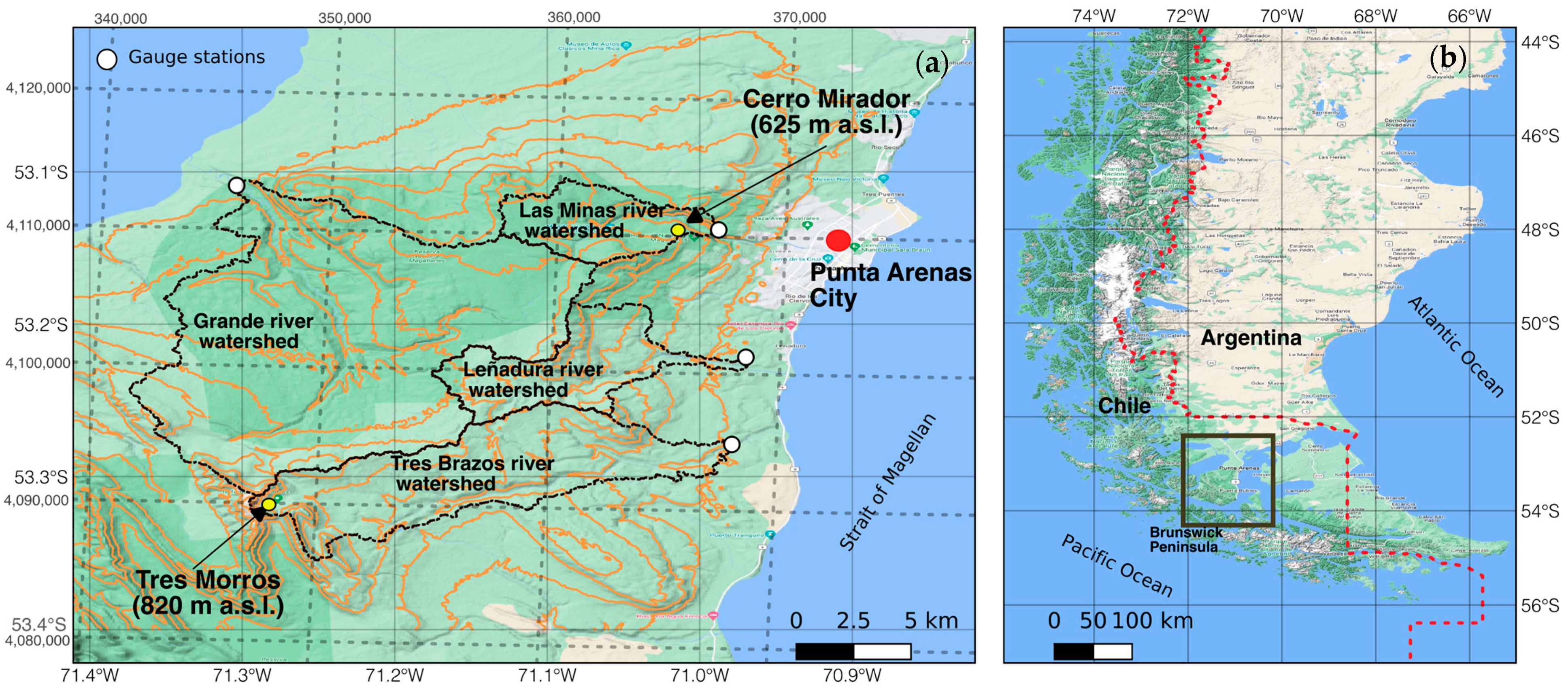
2. Study Area
3. Data and Methods
3.1. Data
3.1.1. Satellite Sensor Data
3.1.2. Weather Stations
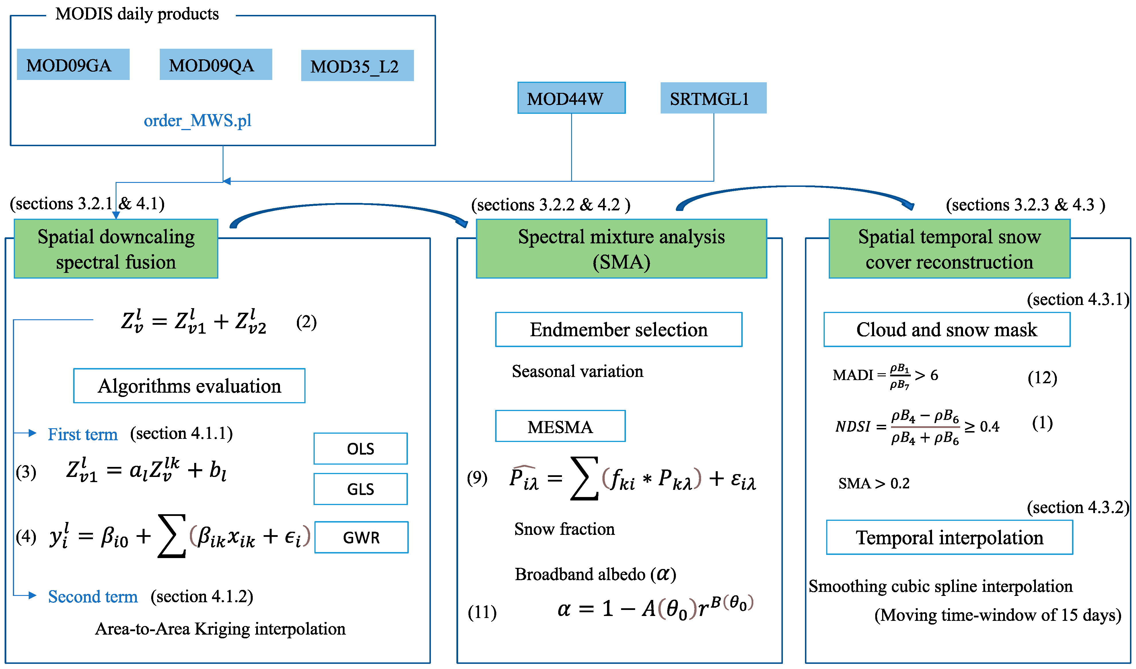
3.2. Methods
3.2.1. Downscaling and Spectral Fusion
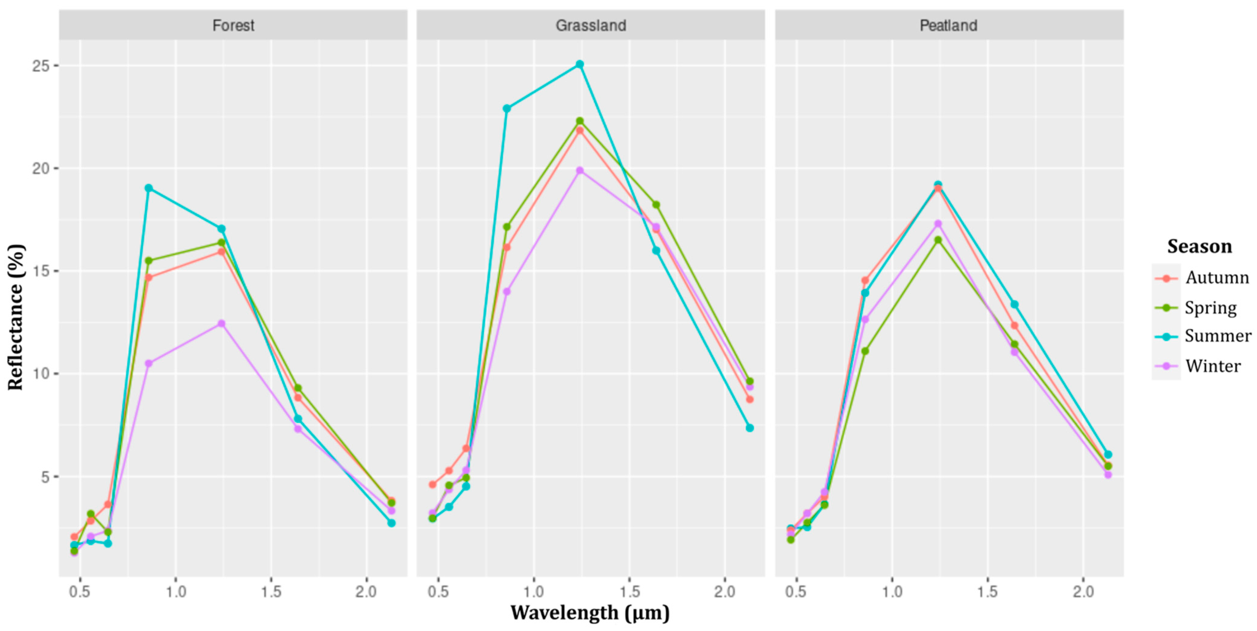
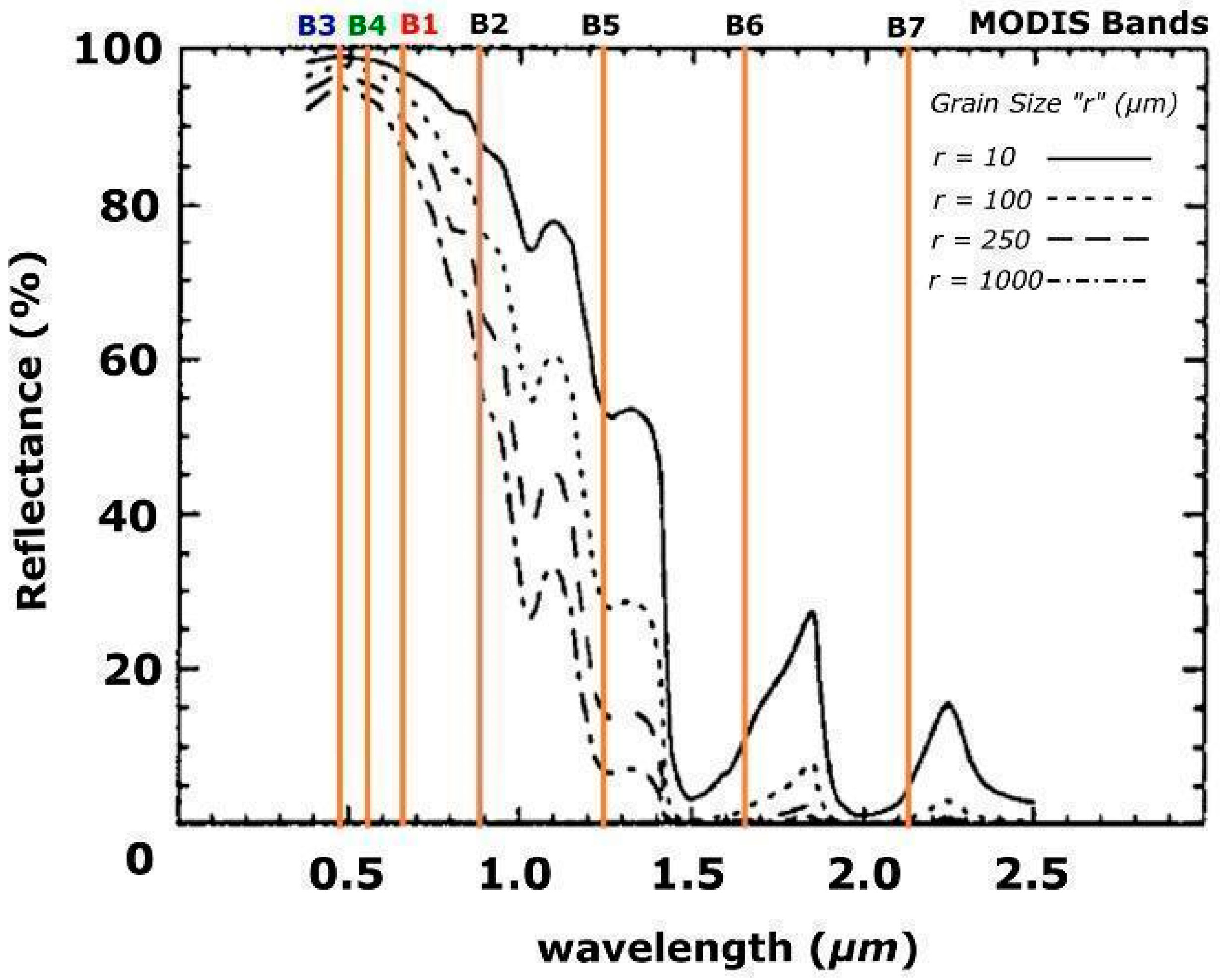
3.2.2. Spectral Mixture Analysis
3.2.3. Spatio-Temporal Snow Reconstruction
- (a)
- Cloud and snow masks
- (b)
- Temporal interpolation
3.2.4. Ground Validation
3.2.5. Snow Cover Variability
4. Results
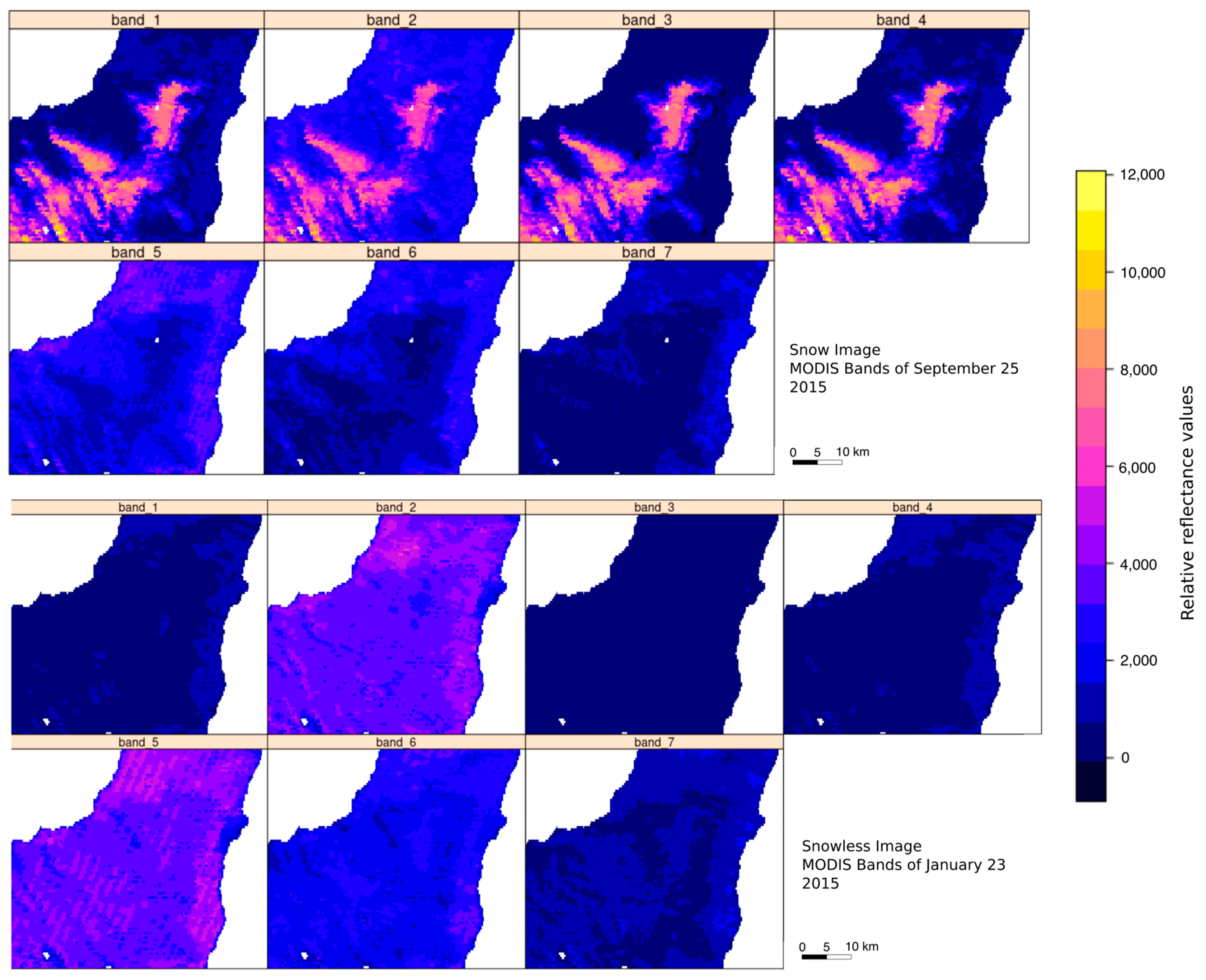
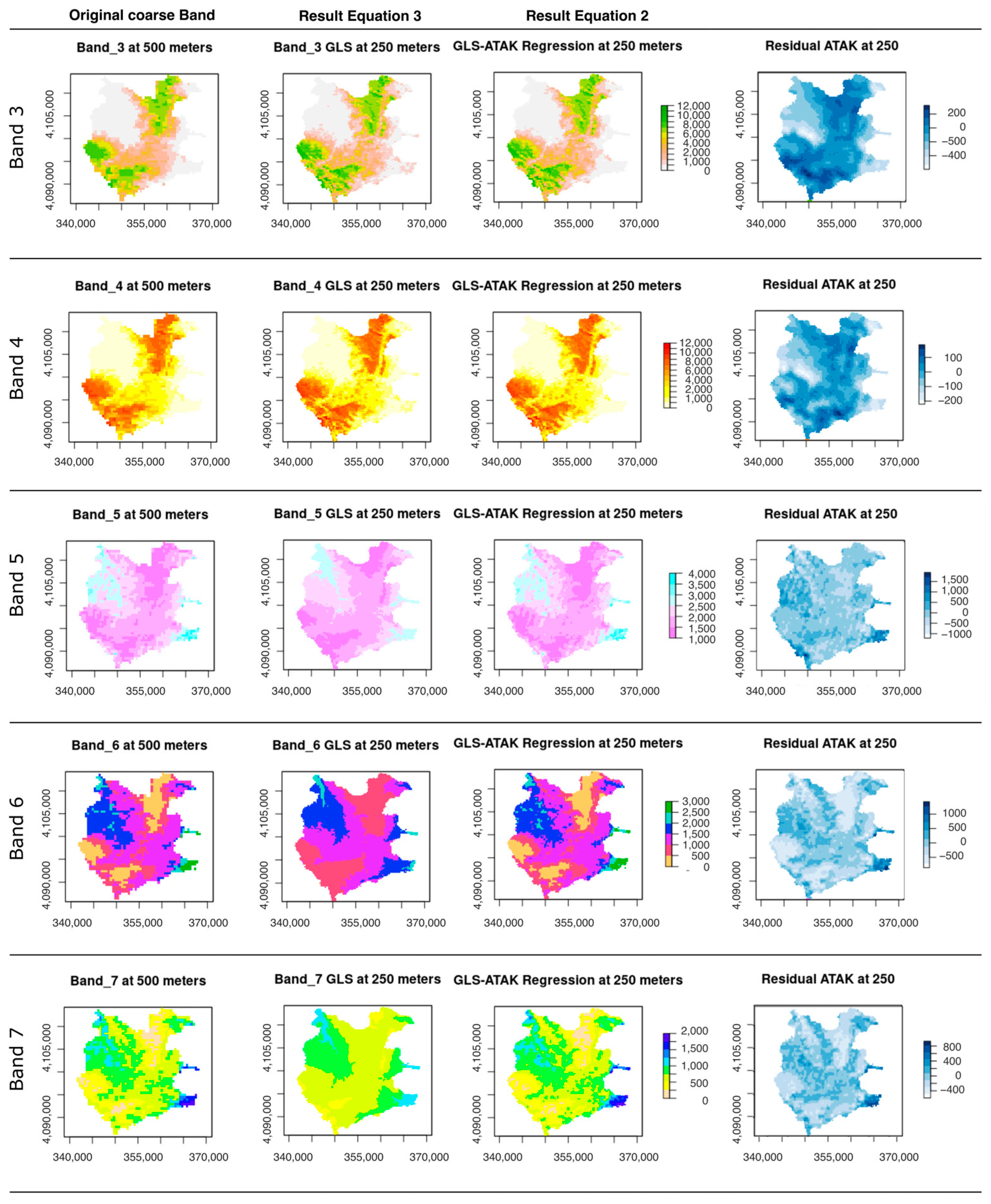
4.1. Spectral Fusion
4.1.1. The First Term of Spectral Fusion: The Linear Relationship
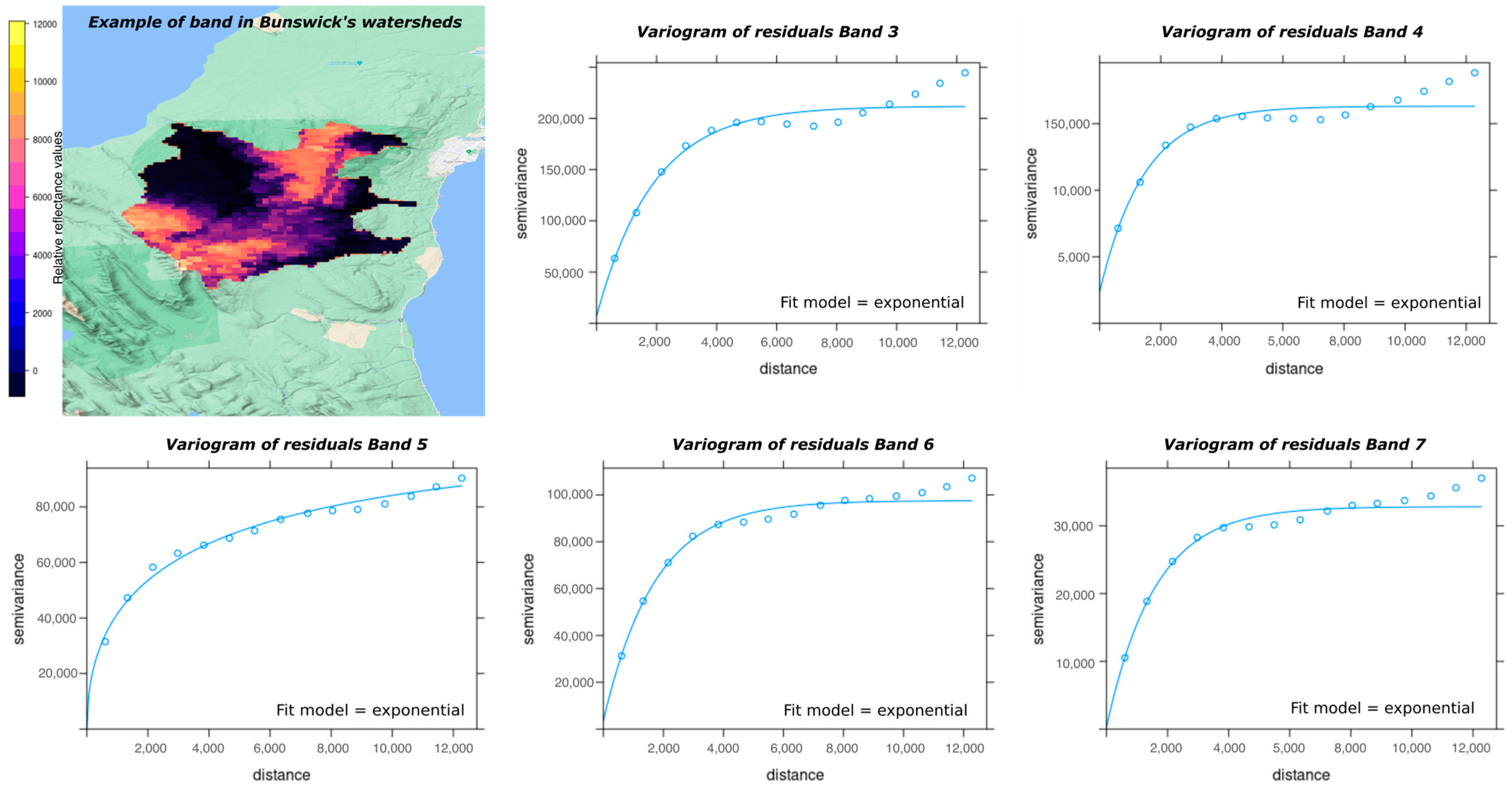
4.1.2. The Second Term of Spectral Fusion: The Kriging Interpolation
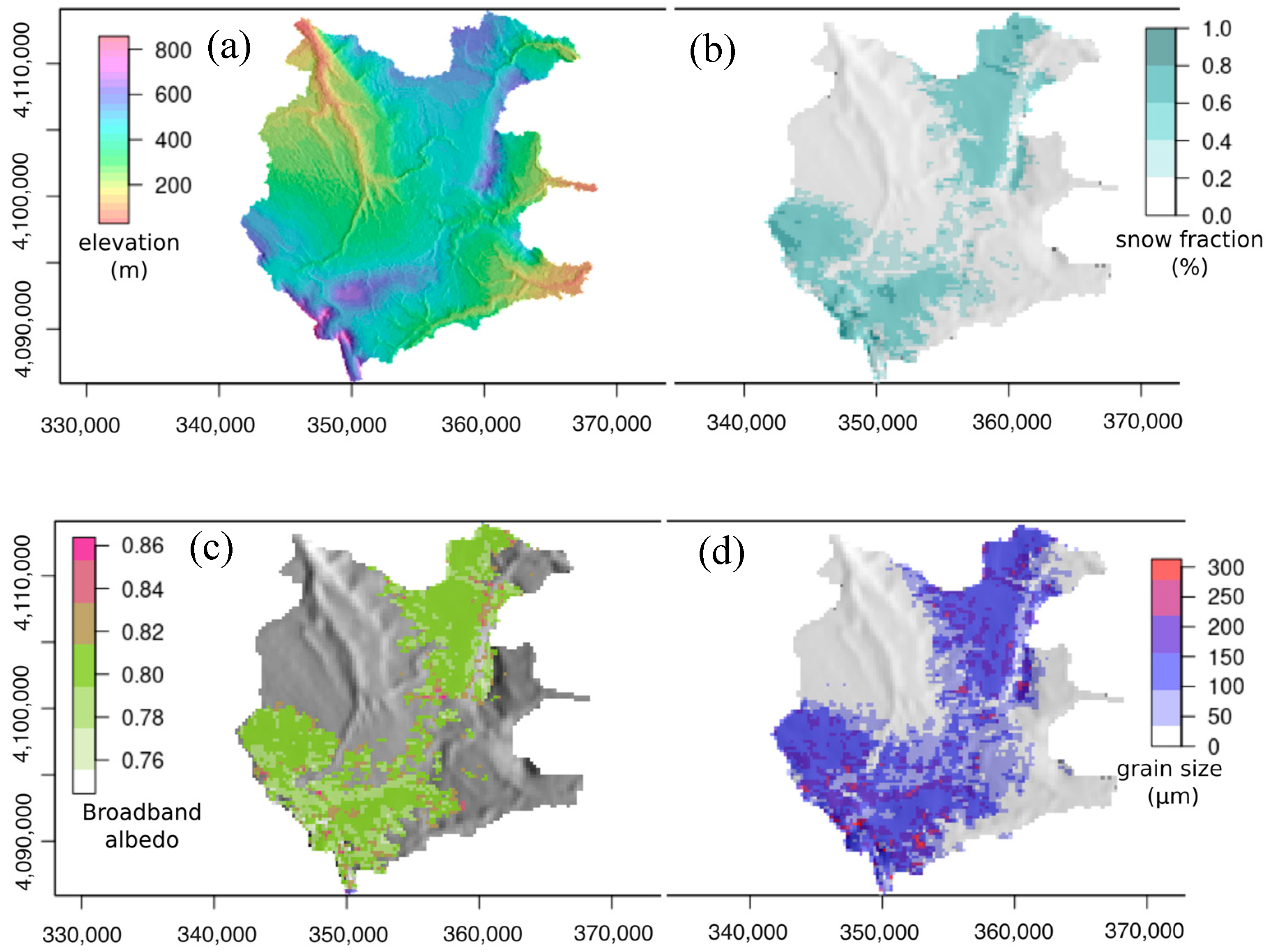
4.2. SMA
4.3. Spatio-Temporal Snow Reconstruction
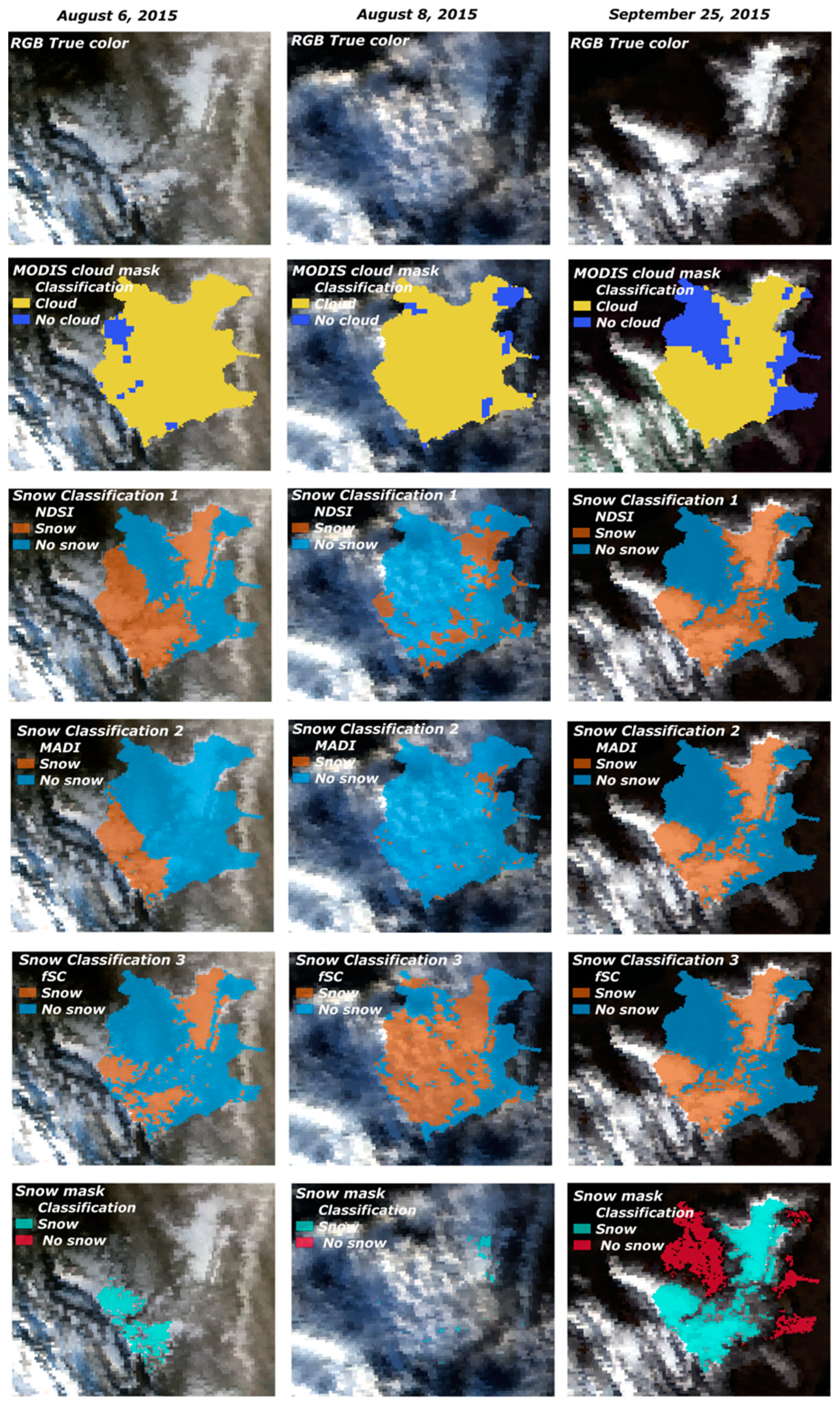
4.3.1. Cloud and Snow Masks
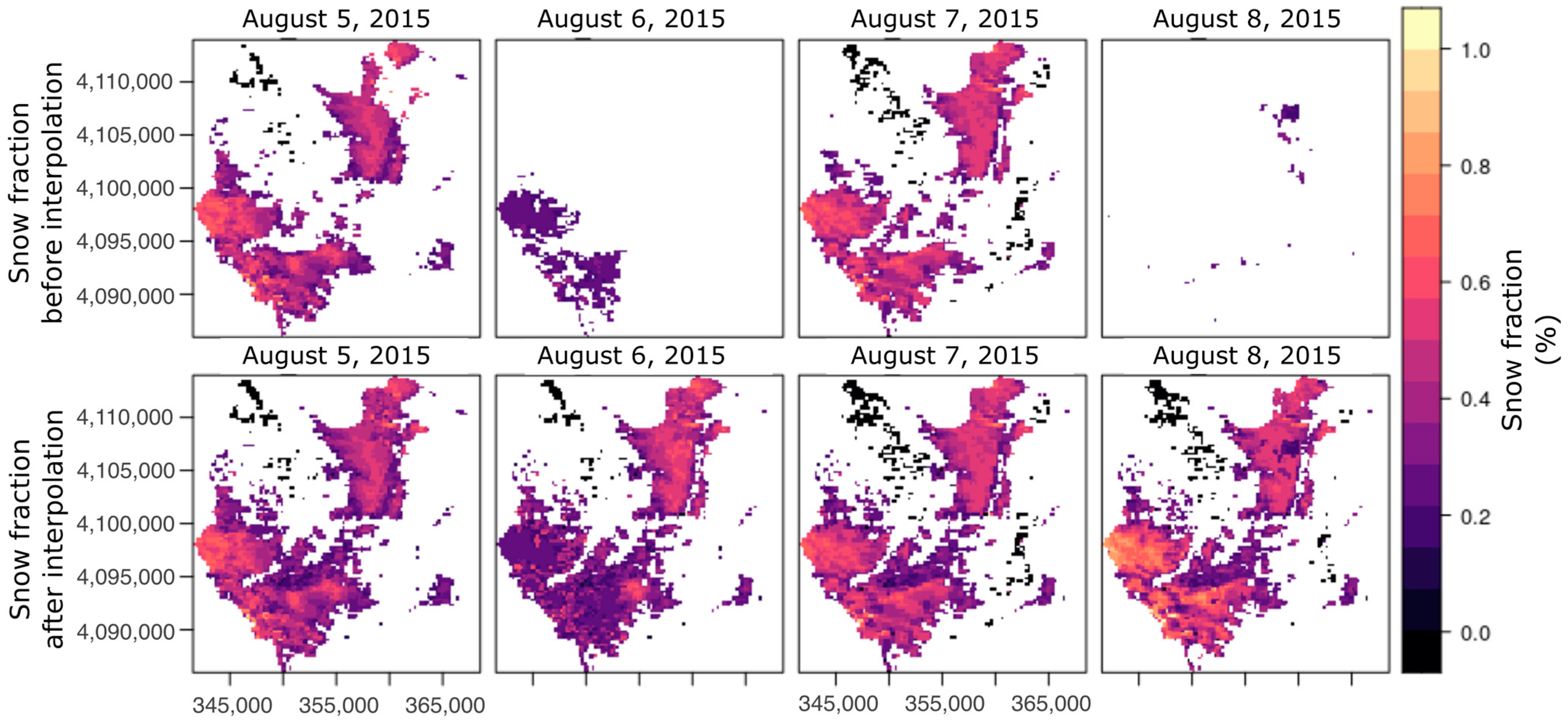
4.3.2. Temporal Interpolation
4.4. Ground Validation with AWS Data
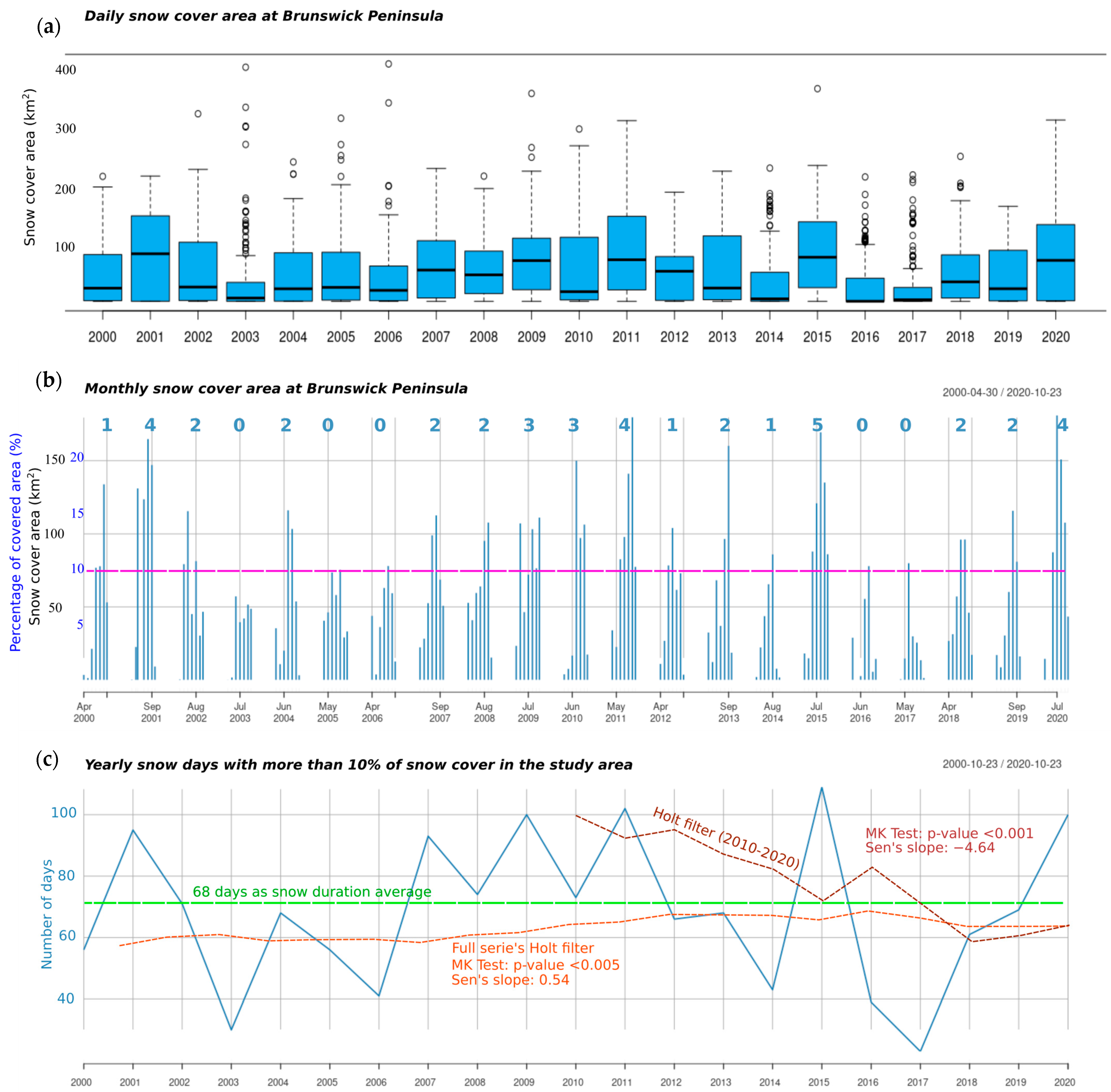
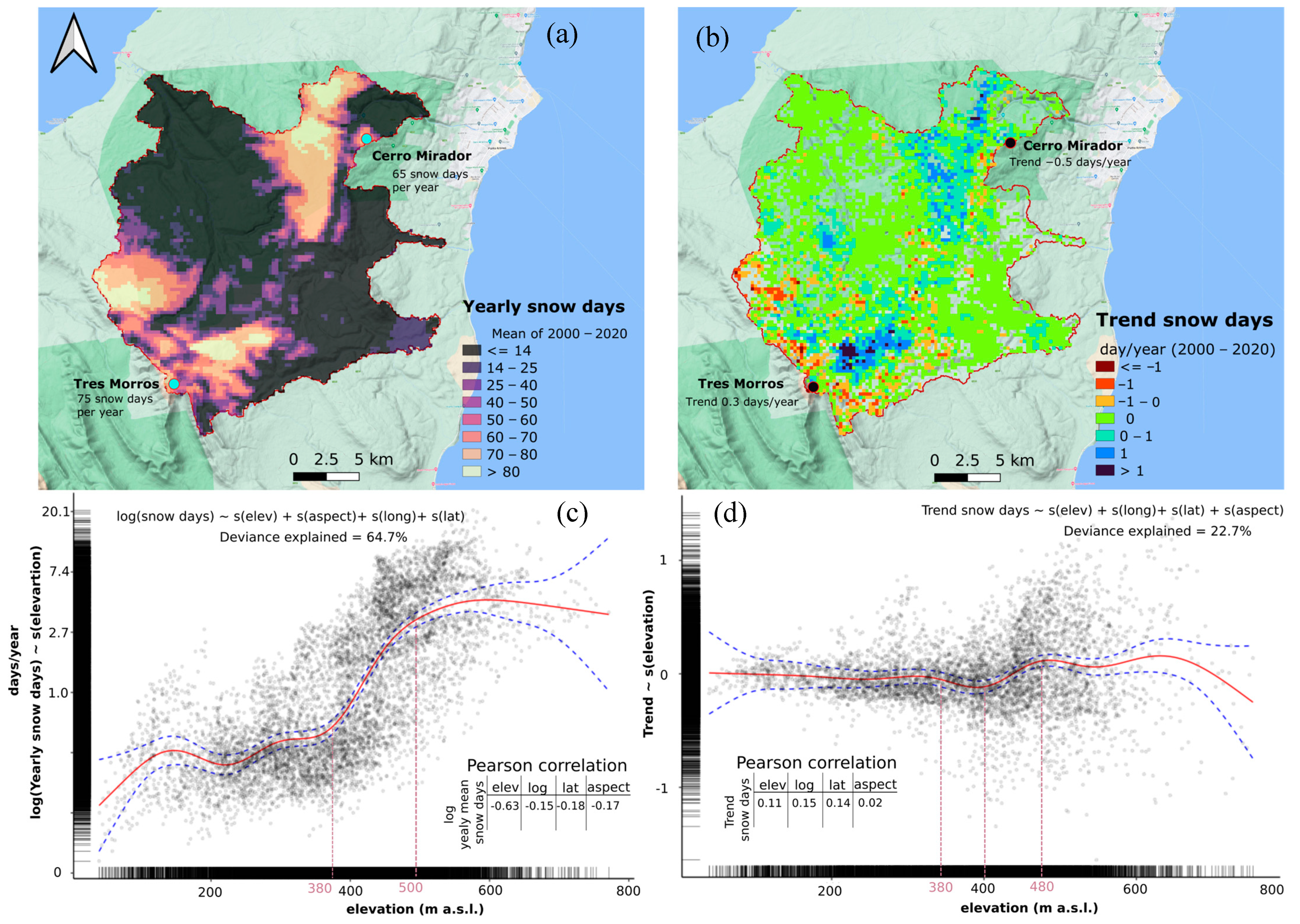
4.5. Reconstructed Snow Cover Variability in the Brunswick Peninsula
5. Discussion
5.1. Method Improvement
5.2. Climatic Forcing
6. Conclusions
Supplementary Materials
Author Contributions
Funding
Data Availability Statement
Acknowledgments
Conflicts of Interest
References
- Chen, X.; Long, D.; Liang, S.; He, L.; Zeng, C.; Hao, X.; Hong, Y. Developing a Composite Daily Snow Cover Extent Record over the Tibetan Plateau from 1981 to 2016 Using Multisource Data. Remote Sens. Environ. 2018, 215, 284–299. [Google Scholar] [CrossRef]
- Frei, A.; Tedesco, M.; Lee, S.; Foster, J.; Hall, D.K.; Kelly, R.; Robinson, D.A. A Review of Global Satellite-Derived Snow Products. Adv. Space Res. 2012, 50, 1007–1029. [Google Scholar] [CrossRef]
- Aguirre, F.; Carrasco, J.; Sauter, T.; Schneider, C.; Gaete, K.; Garín, E.; Adaros, R.; Butorovic, N.; Jaña, R.; Casassa, G. Snow Cover Change as a Climate Indicator in Brunswick Peninsula, Patagonia. Front. Earth Sci. 2018, 6, 130. [Google Scholar]
- Hughes, L. Climate Change and Australia: Trends, Projections and Impacts. Austral Ecol. 2003, 28, 423–443. [Google Scholar] [CrossRef]
- Beniston, M.; Farinotti, D.; Stoffel, M.; Andreassen, L.M.; Coppola, E.; Eckert, N.; Fantini, A.; Giacona, F.; Hauck, C.; Huss, M.; et al. The European Mountain Cryosphere: A Review of Its Current State, Trends, and Future Challenges. Cryosphere 2018, 12, 759–794. [Google Scholar] [CrossRef]
- IPCC Summary for Policymakers. Climate Change 2013: The Physical Science Basis. Contribution of Working Group I to the Fifth Assessment Report of the Intergovernmental Panel on Climate Change; Cambridge University Press: Cambridge, UK, 2013; p. 33. [Google Scholar] [CrossRef]
- Mernild, S.H.; Liston, G.E.; Hiemstra, C.A.; Malmros, J.K.; Yde, J.C.; McPhee, J. The Andes Cordillera. Part I: Snow Distribution, Properties, and Trends (1979–2014). Int. J. Climatol. 2017, 37, 1680–1698. [Google Scholar] [CrossRef]
- Walker, D.A.; Halfpenny, J.C.; Walker, M.D.; Wessman, C.A. Long-Term Studies of Snow-Vegetation Interactions. Bioscience 1993, 43, 287–301. [Google Scholar] [CrossRef]
- Lillesand, T.M.; Kiefer, R.W.; Chipman, J.W. Remote Sensing and Image Interpretation, 7th ed.; John Wiley & Sons: Hoboken, NJ, USA, 2015; ISBN 9781118343289. [Google Scholar]
- Tedesco, M. Electromagnetic Properties of Components of the Cryosphere. In Remote Sensing of the Cryosphere; Tedesco, M., Knight, P., Eds.; Wiley-Blackwell: Oxford, UK, 2014; pp. 17–29. ISBN 9781118368862. [Google Scholar]
- Cortés, G.; Girotto, M.; Margulis, S.A. Analysis of Sub-Pixel Snow and Ice Extent over the Extratropical Andes Using Spectral Unmixing of Historical Landsat Imagery. Remote Sens. Environ. 2014, 141, 64–78. [Google Scholar] [CrossRef]
- Painter, T.H.; Rittger, K.; McKenzie, C.; Slaughter, P.; Davis, R.E.; Dozier, J. Retrieval of Subpixel Snow Covered Area, Grain Size, and Albedo from MODIS. Remote Sens. Environ. 2009, 113, 868–879. [Google Scholar] [CrossRef]
- Rittger, K.; Painter, T.H.; Dozier, J. Assessment of Methods for Mapping Snow Cover from MODIS. Adv. Water Resour. 2013, 51, 367–380. [Google Scholar] [CrossRef]
- Hall, D.K.; Frei, A.; Dery, S. Remote Sensing of Snow Extent. In Remote Sensing of the Cryosphere; Tedesco, M., Knight, P., Eds.; Wiley-Blackwell: Oxford, UK, 2014; pp. 31–47. ISBN 9781118368862. [Google Scholar]
- Hall, D.K.; Riggs, G.A. Accuracy Assessment of the MODIS Snow Products. Hydrol. Process 2007, 21, 1534–1547. [Google Scholar] [CrossRef]
- Riggs, G.; Hall, D. MODIS Snow Products User Guide to Collection 6; National Snow and Ice Data Center: Boulder, CO, USA, 2017. [Google Scholar]
- Hall, D.K.; Riggs, G.A. Normalized-Difference Snow Index (NDSI). In Encyclopedia of Snow, Ice and Glaciers; Singh, V.P., Singh, P., Haritashya, U.K., Eds.; Springer: Dordrecht, The Netherlands; Zurich, Switzerland, 2011; pp. 779–780. [Google Scholar]
- Frei, A.; Lee, S. A Comparison of Optical-Band Based Snow Extent Products during Spring over North America. Remote Sens. Environ. 2010, 114, 1940–1948. [Google Scholar] [CrossRef]
- Hall, D.K.; Riggs, G.A.; Salomonson, V.V.; DiGirolamo, N.E.; Bayr, K.J. MODIS Snow-Cover Products. Remote Sens. Environ. 2002, 83, 181–194. [Google Scholar] [CrossRef]
- Lopez, P.; Sirguey, P.; Arnaud, Y.; Pouyaud, B.; Chevallier, P. Snow Cover Monitoring in the Northern Patagonia Icefield Using MODIS Satellite Images (2000–2006). Glob. Planet. Change 2008, 61, 103–116. [Google Scholar] [CrossRef]
- Sirguey, P.; Mathieu, R.; Arnaud, Y. Subpixel Monitoring of the Seasonal Snow Cover with MODIS at 250 m Spatial Resolution in the Southern Alps of New Zealand: Methodology and Accuracy Assessment. Remote Sens. Environ. 2009, 113, 160–181. [Google Scholar] [CrossRef]
- Musselman, K.N.; Molotch, N.P.; Brooks, P.D. Effects of Vegetation on Snow Accumulation and Ablation in a Mid-Latitude Sub-Alpine Forest. Hydrol. Process 2008, 22, 2767–2776. [Google Scholar] [CrossRef]
- Varhola, A.; Coops, N.C.; Weiler, M.; Moore, R.D. Forest Canopy Effects on Snow Accumulation and Ablation: An Integrative Review of Empirical Results. J. Hydrol. 2010, 392, 219–233. [Google Scholar] [CrossRef]
- Dumont, M.; Gardelle, J.; Sirguey, P.; Guillot, A.; Six, D.; Rabatel, A.; Arnaud, Y. Linking Glacier Annual Mass Balance and Glacier Albedo Retrieved from MODIS Data. Cryosphere 2012, 6, 1527–1539. [Google Scholar] [CrossRef]
- WMO; UNESCO; UNEP; ICSU. Systematic Observation Requirements for Satellite-Based Data Products for Climate 2011 Update: Supplemental Details to the Satellite-Based Component of the “Implementation Plan for the Global Observing System for Climate in Support of the UNFCCC; 2010 Update; World Meteorological Organisation (WMO): Geneva, Switzerland, 2011. [Google Scholar]
- Dozier, J.; Painter, T.H. Multispectral and hyperspectral remote sensing of alpine snow properties. Annu. Rev. Earth Planet. Sci. 2004, 32, 465–494. [Google Scholar] [CrossRef]
- Pérez, T.; Mattar, C.; Fuster, R. Decrease in Snow Cover over the Aysén River Catchment in Patagonia, Chile. Water 2018, 10, 619. [Google Scholar] [CrossRef]
- Stehr, A.; Aguayo, M. Snow Cover Dynamics in Andean Watersheds of Chile (32.0–39.5°S) during the Years 2000–2016. Hydrol. Earth Syst. Sci. 2017, 21, 5111–5126. [Google Scholar] [CrossRef]
- Malmros, J.K.; Mernild, S.H.; Wilson, R.; Tagesson, T.; Fensholt, R. Snow Cover and Snow Albedo Changes in the Central Andes of Chile and Argentina from Daily MODIS Observations (2000–2016). Remote Sens. Environ. 2018, 209, 240–252. [Google Scholar] [CrossRef]
- Mernild, S.H.; Beckerman, A.P.; Yde, J.C.; Hanna, E.; Malmros, J.K.; Wilson, R.; Zemp, M. Mass Loss and Imbalance of Glaciers along the Andes Cordillera to the Sub-Antarctic Islands. Glob. Planet. Chang. 2015, 133, 109–119. [Google Scholar] [CrossRef]
- Garreaud, R.; Lopez, P.; Minvielle, M.; Rojas, M.; Garreaud, R.; Lopez, P.; Minvielle, M.; Rojas, M. Large-Scale Control on the Patagonian Climate. J. Clim. 2013, 26, 215–230. [Google Scholar] [CrossRef]
- Rozzi, R.; Massardo, F.; Gallardo, M.R.; Plana, J. La Reserva de Biosfera Cabo de Hornos: Un Desafío Para La Conservación de La Biodiversidad e Implementación del Desarrollo Sustentable en El Extremo Austral de América. Environ. Res. 2007, 35, 55–70. [Google Scholar]
- Aguirre, F.; Squeo, F.A.; López, D.; Grego, R.D.; Buma, B.; Carvajal, D.; Jaña, R.; Casassa, G.; Rozzi, R. Gradientes Climáticos y su Alta Influencia en los Ecosistemas Terrestres de la Reserva de La Biosfera Cabo de Hornos, Chile. In Anales del Instituto de la Patagonia; Universidad de Magallanes: Punta Arenas, Chile, 2021; Volume 49. [Google Scholar] [CrossRef]
- Aravena, J.C.; Luckman, B.H. Spatio-Temporal Rainfall Patterns in Southern South America. Int. J. Climatol. 2009, 29, 2106–2120. [Google Scholar] [CrossRef]
- Davies, B.J.; Darvill, C.M.; Lovell, H.; Bendle, J.M.; Dowdeswell, J.A.; Fabel, D.; García, J.L.; Geiger, A.; Glasser, N.F.; Gheorghiu, D.M.; et al. The Evolution of the Patagonian Ice Sheet from 35 Ka to the Present Day (PATICE). Earth Sci. Rev. 2020, 204, 103152. [Google Scholar] [CrossRef]
- Kilian, R.; Lamy, F. A Review of Glacial and Holocene Paleoclimate Records from Southernmost Patagonia (49–55°S). Quat. Sci. Rev. 2012, 53, 1–23. [Google Scholar] [CrossRef]
- Markgraf, V.; Huber, U.M. Late and Postglacial Vegetation and Fire History in Southern Patagonia and Tierra Del Fuego. Palaeogeogr. Palaeoclimatol. Palaeoecol. 2010, 297, 351–366. [Google Scholar] [CrossRef]
- Villalba, R.; Grosjean, M.; Kiefer, T. Long-Term Multi-Proxy Climate Reconstructions and Dynamics in South America (LOTRED-SA): State of the Art and Perspectives. Palaeogeogr. Palaeoclimatol. Palaeoecol. 2009, 281, 175–179. [Google Scholar] [CrossRef]
- Mayewski, P.A.; Meredith, M.P.; Summerhayes, C.P.; Turner, J.; Worby, A.; Barrett, P.J.; Casassa, G.; Bertler, N.A.N.; Bracegirdle, T.; Naveira Garabato, A.C.; et al. State of the Antarctic and Southern Ocean Climate System. Rev. Geophys. 2009, 47, RG1003. [Google Scholar] [CrossRef]
- Marshall, G.J. Trends in the Southern Annular Mode from Observations and Reanalyses. J. Clim. 2003, 16, 4134–4143. [Google Scholar] [CrossRef]
- Sauter, T. Revisiting Extreme Precipitation Amounts over Southern South America and Implications for the Patagonian Icefields. Hydrol. Earth Syst. Sci. 2020, 24, 2003–2016. [Google Scholar] [CrossRef]
- Carrasco, J.F.; Casassa, G.; Rivera, A. Meteorological and Climatological Aspects of the Southern Patagonia Icefield; Springer: Boston, MA, USA, 2002; pp. 29–41. [Google Scholar]
- Schneider, C.; Glaser, M.; Kilian, R.; Santana, A.; Butorovic, N.; Casassa, G. Weather Observations Across the Southern Andes at 53° S. Phys. Geogr. 2003, 24, 97–119. [Google Scholar] [CrossRef]
- Weidemann, S.S.; Sauter, T.; Kilian, R.; Steger, D.; Butorovic, N.; Schneider, C. A 17-Year Record of Meteorological Observations Across the Gran Campo Nevado Ice Cap in Southern Patagonia, Chile, Related to Synoptic Weather Types and Climate Modes. Front. Earth Sci. 2018, 6, 53. [Google Scholar] [CrossRef]
- Alvarez-Garreton, C.; Mendoza, P.A.; Boisier, J.P.; Addor, N.; Galleguillos, M.; Zambrano-Bigiarini, M.; Lara, A.; Cortes, G.; Garreaud, R.; McPhee, J. The CAMELS-CL Dataset: Catchment Attributes and Meteorology for Large Sample Studies-Chile Dataset. Hydrol. Earth Syst. Sci. 2018, 22, 5817–5846. [Google Scholar] [CrossRef]
- Farr, T.G.; Rosen, P.A.; Caro, E.; Crippen, R.; Duren, R.; Hensley, S.; Kobrick, M.; Paller, M.; Rodriguez, E.; Roth, L.; et al. The Shuttle Radar Topography Mission. Rev. Geophys. 2007, 45, RG2004. [Google Scholar] [CrossRef]
- Painter, T.H.; Roberts, D.A.; Green, R.O.; Dozier, J. The Effect of Grain Size on Spectral Mixture Analysis of Snow-Covered Area from AVIRIS Data. Remote Sens. Environ. 1998, 65, 320–332. [Google Scholar] [CrossRef]
- Pohl, C.; Van Genderen, J. Remote Sensing Image Fusion: A Practical Guide; CRC Press: Boca Raton, FL, USA, 2017; ISBN 1498730035. [Google Scholar]
- Canty, M.J. Image Analysis, Classification and Change Detection in Remote Sensing: With Algorithms for Python, 4th ed.; CRC Press: Boca Raton, FL, USA, 2019; ISBN 0429875347. [Google Scholar]
- Shettigara, V.K. A Generalized Component Substitution Technique for Spatial Enhancement of Multispectral Images Using a Higher Resolution Data Set. Photogramm. Eng. Remote Sens. 1992, 58, 561–567. [Google Scholar]
- Nunez, J.; Otazu, X.; Fors, O.; Prades, A.; Pala, V.; Arbiol, R. Multiresolution-Based Image Fusion with Additive Wavelet Decomposition. IEEE Trans. Geosci. Remote Sens. 1999, 37, 1204–1211. [Google Scholar] [CrossRef]
- Ranchin, T.; Aiazzi, B.; Alparone, L.; Baronti, S.; Wald, L. Image Fusion—The ARSIS Concept and Some Successful Implementation Schemes. ISPRS J. Photogramm. Remote Sens. 2003, 58, 4–18. [Google Scholar] [CrossRef]
- Aiazzi, B.; Alparone, L.; Baronti, S.; Garzelli, A. Context-Driven Fusion of High Spatial and Spectral Resolution Images Based on Oversampled Multiresolution Analysis. IEEE Trans. Geosci. Remote Sens. 2002, 40, 2300–2312. [Google Scholar] [CrossRef]
- Sales, M.H.; Souza, C.M.; Kyriakidis, P.C. Fusion of MODIS Images Using Kriging With External Drift. IEEE Trans. Geosci. Remote Sens. 2013, 51, 2250–2259. [Google Scholar] [CrossRef]
- Wang, Q.; Shi, W.; Atkinson, P.M.; Zhao, Y. Downscaling MODIS Images with Area-to-Point Regression Kriging. Remote Sens. Environ. 2015, 166, 191–204. [Google Scholar] [CrossRef]
- Gao, F.; Kustas, W.; Anderson, M. A Data Mining Approach for Sharpening Thermal Satellite Imagery over Land. Remote Sens. 2012, 4, 3287–3319. [Google Scholar] [CrossRef]
- Hu, M.; Huang, Y. Atakrig: An R Package for Multivariate Area-to-Area and Area-to-Point Kriging Predictions. Comput. Geosci. 2020, 139, 104471. [Google Scholar] [CrossRef]
- Pardo-Iguzquiza, E.; Atkinson, P.M.; Chica-Olmo, M. DSCOKRI: A Library of Computer Programs for Downscaling Cokriging in Support of Remote Sensing Applications. Comput. Geosci. 2010, 36, 881–894. [Google Scholar] [CrossRef]
- Jin, Y.; Ge, Y.; Wang, J.; Heuvelink, G.; Wang, L. Geographically Weighted Area-to-Point Regression Kriging for Spatial Downscaling in Remote Sensing. Remote Sens. 2018, 10, 579. [Google Scholar] [CrossRef]
- Zuur, A.; Ieno, E.N.; Walker, N.; Saveliev, A.A.; Smith, G.M. Dealing with Heterogeneity. In Mixed Effects Models and Extensions in Ecology with R; Springer Science & Business Media: Berlin/Heidelberg, Germany, 2009; pp. 71–101. ISBN 0387874585. [Google Scholar]
- Hijmans, R.J.; van Etten, J. Raster: Geographic Data Analysis and Modeling, R Package Version 3.6-23. 2023. Available online: https://libraries.io/cran/raster (accessed on 8 August 2023).
- Pinheiro, J.; Bates, D.; DebRoy, S.; Sarkar, D.; Heisterkamp, S.; Van Willigen, B.; Maintainer, R. Package ‘Nlme.’ Linear and Nonlinear Mixed Effects Models, R Package Version 3.1-163. 2023. Available online: https://www.rdocumentation.org/packages/nlme/versions/3.1-163 (accessed on 8 August 2023).
- Pebesma, E.J. Multivariable Geostatistics in S: The Gstat Package. Comput. Geosci. 2004, 30, 683–691. [Google Scholar] [CrossRef]
- Gollini, I.; Lu, B.; Charlton, M.; Brunsdon, C.; Harris, P. GWmodel: An R Package for Exploring Spatial Heterogeneity Using Geographically Weighted Models. J. Stat. Softw. 2013, 63, 1–50. [Google Scholar] [CrossRef]
- Wang, Z.; Bovik, A.C. A Universal Image Quality Index. IEEE Signal Process. Lett. 2002, 9, 81–84. [Google Scholar] [CrossRef]
- Alparone, L.; Aiazzi, B.; Baronti, S.; Garzelli, A.; Nencini, F.; Selva, M. Multispectral and Panchromatic Data Fusion Assessment without Reference. Photogramm. Eng. Remote Sens. 2008, 74, 193–200. [Google Scholar] [CrossRef]
- Somers, B.; Asner, G.P.; Tits, L.; Coppin, P. Endmember Variability in Spectral Mixture Analysis: A Review. Remote Sens. Environ. 2011, 115, 1603–1616. [Google Scholar] [CrossRef]
- Roberts, D.A.; Gardner, M.; Church, R.; Ustin, S.; Scheer, G.; Green, R.O. Mapping Chaparral in the Santa Monica Mountains Using Multiple Endmember Spectral Mixture Models. Remote Sens. Environ. 1998, 65, 267–279. [Google Scholar] [CrossRef]
- Leutner, B.; Horning, N.; Schwalb-Willmann, J.; Hijmans, R.J. RStoolbox: Tools for Remote Sensing Data Analysis, R package version 0.2.6. 2019. Available online: https://bleutner.github.io/RStoolbox/ (accessed on 8 August 2023).
- Dudley, K.L.; Roth, K.L.; Coates, A.R. A Multi-Temporal Spectral Library Approach for Mapping Vegetation Species across Spatial and Temporal Phenological Gradients. Remote Sens. Environ. 2015, 167, 121–134. [Google Scholar] [CrossRef]
- Congedo, L. Semi-Automatic Classification Plugin Documentation. Release 2016, 4, 29. [Google Scholar]
- QGIS Development-Teams. QGIS Geographic Information System. QGIS Association. 2023. Available online: https://www.qgis.org (accessed on 8 August 2023).
- Dozier, J.; Painter, T.H.; Rittger, K.; Frew, J.E. Time-Space Continuity of Daily Maps of Fractional Snow Cover and Albedo from MODIS. Adv. Water Resour. 2008, 31, 1515–1526. [Google Scholar] [CrossRef]
- Redpath, T.A.N.; Sirguey, P.; Cullen, N.J. Characterising Spatio-Temporal Variability in Seasonal Snow Cover at a Regional Scale from MODIS Data: The Clutha Catchment, New Zealand. Hydrol. Earth Syst. Sci. 2019, 23, 3189–3217. [Google Scholar] [CrossRef]
- Chylek, P.; McCabe, M.; Dubey, M.K.; Dozier, J. Remote Sensing of Greenland Ice Sheet Using Multispectral Near-Infrared and Visible Radiances. J. Geophys. Res. 2007, 112, D24S20. [Google Scholar] [CrossRef]
- Bormann, K.J.; McCabe, M.F.; Evans, J.P. Satellite Based Observations for Seasonal Snow Cover Detection and Characterisation in Australia. Remote Sens. Environ. 2012, 123, 57–71. [Google Scholar] [CrossRef]
- de Medeiros, E.S.; de Lima, R.R.; de Olinda, R.A.; Dantas, L.G.; dos Santos, C.A.C. Space–Time Kriging of Precipitation: Modeling the Large-Scale Variation with Model GAMLSS. Water 2019, 11, 2368. [Google Scholar] [CrossRef]
- Wang, Y. Smoothing Splines: Methods and Applications; CRC Press: Boca Raton, FL, USA, 2011; ISBN 1420077562. [Google Scholar]
- Pebesma, E. Spacetime: Spatio-Temporal Data in R. J. Stat. Softw. 2012, 51, 1–30. [Google Scholar] [CrossRef]
- Easterling, D.R.; Kunkel, K.E.; Wehner, M.F.; Sun, L. Detection and Attribution of Climate Extremes in the Observed Record. Weather. Clim. Extrem. 2016, 11, 17–27. [Google Scholar] [CrossRef]
- Mudelsee, M. Trend Analysis of Climate Time Series: A Review of Methods. Earth Sci. Rev. 2019, 190, 310–322. [Google Scholar] [CrossRef]
- Rodell, M.; Houser, P.R. Updating a Land Surface Model with MODIS-Derived Snow Cover. J. Hydrometeorol. 2004, 5, 1064–1075. [Google Scholar] [CrossRef]
- Wood, S.N. Generalized Additive Models: An Introduction with R2 An Introduction with R. Gen. Addit. Models 2017, 10, 9781315370279. [Google Scholar]
- Mann, B.H. Non-Parametric Test Against Trend. Econometrica 1945, 13, 245–259. [Google Scholar] [CrossRef]
- Sen, P.K. Estimates of the Regression Coefficient Based on Kendall’s Tau. J. Am. Stat. Assoc. 1968, 63, 1379–1389. [Google Scholar] [CrossRef]
- Helsel, D.R.; Hirsch, R.M. Echniques of Water Resources Investigations; Book 4, Chapter A3; U.S. Geological Survey: Reston, VA, USA, 2002; ISBN 0444814639/9780444814630.
- Rosenbluth, B.N.; Fuenzalida, H.A.; Aceituno, P. Recent Temperature Variations in Southern South America. Int. J. Climatol. 1997, 17, 67–85. [Google Scholar] [CrossRef]
- Hyndman, R.; Koehler, A.B.; Ord, J.K.; Snyder, R.D. Forecasting with Exponential Smoothing: The State Space Approach. Springer Science & Business Media: Berlin/Heidelberg, Germany, 2008; ISBN 3540719180. [Google Scholar]
- Chatfield, C. The Analysis of Time Series: An Introduction, 6th ed.; CRC Press: Boca Raton, FL, USA, 2003. [Google Scholar] [CrossRef]
- Jassby, A.D.; Cloern, J.E. Wq: Exploring Water Quality Monitoring Data, R package version 1.0.0. 2022. Available online: https://github.com/jsta/wql/releases/tag/v1.0.0 (accessed on 8 August 2023).
- Frey, R.A.; Ackerman, S.A.; Liu, Y.; Strabala, K.I.; Zhang, H.; Key, J.R.; Wang, X. Cloud Detection with MODIS. Part I: Improvements in the MODIS Cloud Mask for Collection 5. J. Atmos. Ocean. Technol. 2008, 25, 1057–1072. [Google Scholar] [CrossRef]
- Srur, A.M.; Villalba, R.; Rodríguez-Catón, M.; Amoroso, M.M.; Marcotti, E. Climate and Nothofagus Pumilio Establishment at Upper Treelines in the Patagonian Andes. Front. Earth Sci. 2018, 6, 57. [Google Scholar] [CrossRef]
- Sato, K.; Inoue, J. Comparison of Arctic Sea Ice Thickness and Snow Depth Estimates from CFSR with in Situ Observations. Clim. Dyn. 2018, 50, 289–301. [Google Scholar] [CrossRef]
- Wang, C.; Graham, R.M.; Wang, K.; Gerland, S.; Granskog, M.A. Comparison of ERA5 and ERA-Interim near-Surface Air Temperature, Snowfall and Precipitation over Arctic Sea Ice: Effects on Sea Ice Thermodynamics and Evolution. Cryosphere 2019, 13, 1661–1679. [Google Scholar] [CrossRef]
- Cao, B.; Arduini, G.; Zsoter, E. Brief Communication: Improving ERA5-Land Soil Temperature in Permafrost Regions Using an Optimized Multi-Layer Snow Scheme. Cryosphere 2022, 16, 2701–2708. [Google Scholar] [CrossRef]
- Cao, B.; Gruber, S.; Zheng, D.; Li, X. The ERA5-Land Soil Temperature Bias in Permafrost Regions. Cryosphere 2020, 14, 2581–2595. [Google Scholar] [CrossRef]
- Muñoz-Sabater, J.; Dutra, E.; Agustí-Panareda, A.; Albergel, C.; Arduini, G.; Balsamo, G.; Boussetta, S.; Choulga, M.; Harrigan, S.; Hersbach, H.; et al. ERA5-Land: A State-of-the-Art Global Reanalysis Dataset for Land Applications. Earth Syst. Sci. Data 2021, 13, 4349–4383. [Google Scholar] [CrossRef]
- Bravo, C.; Ross, A.N.; Quincey, D.J.; Cisternas, S.; Rivera, A. Surface Ablation and Its Drivers along a West–East Transect of the Southern Patagonia Icefield. J. Glaciol. 2021, 68, 305–318. [Google Scholar] [CrossRef]
- Quilodrán, C.S.; Sandvig, E.M.; Aguirre, F.; de Aguilar, J.R.; Barroso, O.; Vásquez, R.A.; Rozzi, R. The Extreme Rainfall Gradient of the Cape Horn Biosphere Reserve and its Impact on Forest Bird Richness. Biodivers. Conserv. 2022, 31, 613–627. [Google Scholar] [CrossRef] [PubMed]
- Schaefer, M.; Machguth, H.; Falvey, M.; Casassa, G. Modeling Past and Future Surface Mass Balance of the Northern Patagonia Icefield. J. Geophys. Res. Earth Surf. 2013, 118, 571–588. [Google Scholar] [CrossRef]
- Bozkurt, D.; Rojas, M.; Boisier, J.P.; Rondanelli, R.; Garreaud, R.; Gallardo, L. Dynamical Downscaling over the Complex Terrain of Southwest South America: Present Climate Conditions and Added Value Analysis. Clim. Dyn. 2019, 53, 6745–6767. [Google Scholar] [CrossRef]


| Year | 2010 | 2011 | 2012 | 2013 | 2014 | 2015 | 2016 | 2017 | 2018 | 2019 | 2020 |
|---|---|---|---|---|---|---|---|---|---|---|---|
| Season length | 78 | 85 | 65 | 76 | 57 | 95 | 10 | 0 | 30 | 30 | Closed due to pandemic |
| Snow Image | Snowless Image | |
|---|---|---|
| Bandi | Bandi~Band1 | Bandi~Band1 |
| Band3 | R2 = 0.96 RMSE = 0.229 | R2 = 0.91 RMSE = 0.066 |
| Band4 | R2 = 0.99 RMSE = 0.094 | R2 = 0.84 RMSE = 0.074 |
| Band5 | R2 = 0.39 RMSE = 0.264 | R2 = 0.22 RMSE = 0.165 |
| Band6 | R2 = 0.54 RMSE = 0.229 | R2 = 0.73 RMSE = 0.133 |
| Band7 | R2 = 0.41 RMSE = 0.409 | R2 = 0.93 RMSE = 0.075 |
| Coarse Band | New Relationship Proposed | OLS Regression Results |
|---|---|---|
| Band 3 | R2 = 0.96 RMSE = 0.230 | |
| Band 4 | R2 = 0.99 RMSE = 0.094 | |
| Band 5 | R2 = 0.52 RMSE = 0.234 | |
| Band 6 | R2 = 0.68 RMSE = 0.319 | |
| Band 7 | R2 = 0.61 RMSE = 0.333 |
| OLS500 | GLS500 | GWR500 | OLS_ATAK250 | GLS_ATAK250 | GWR_ATAK250 | |
|---|---|---|---|---|---|---|
| Band_3500 | R2 = 0.97 RMSE = 0.230 AIC = −175 | R2 = 0.97 RMSE = 0.372 AIC = −2877 | R2 = 0.99 RMSE = 0.110 AIC = −2500 | UQI = 0.92 | UQI = 0.94 | UQI = 0.93 |
| Band_4500 | R2 = 0.993 RMSE = 0.085 AIC = −3713 | R2 = 0.993 RMSE = 0.101 AIC = −6053 | R2 = 0.99 RMSE = 0.038 AIC = −6296 | UQI = 0.93 | UQI = 0.93 | UQI = 0.93 |
| Band_5500 | R2 = 0.64 RMSE = 0.152 AIC = −1654 | R2 = 0.63 RMSE = 0.153 AIC =−1727 | R2 = 0.97 RMSE = 0.047 AIC = −5404 | UQI = 0.89 | UQI = 0.98 | UQI = 0.89 |
| Band_6500 | R2 = 0.69 RMSE = 0.304 AIC = 822 | R2 = 0.65 RMSE = 0.392 AIC = 222 | R2 = 0.98 RMSE = 0.074 AIC = −3838 | UQI = 0.96 | UQI = 0.99 | UQI = 0.91 |
| Band_7500 | R2 = 0.58 RMSE = 0.302 AIC = 794 | R2 = 0.53 RMSE = 0.359 AIC = 498 | R2 = 0.97 RMSE = 0.080 AIC = −3545 | UQI = 0.97 | UQI = 0.99 | UQI = 0.89 |
| Ds | 0.042 | 0.043 | 0.039 | |||
| Dγ | 0.015 | 0.009 | 0.016 | |||
| QNR Index | 0.943 | 0.949 | 0.946 |
| Southern Hemisphere Season | Image Date |
|---|---|
| Summer | 17 January 2015 16 January 2016 |
| Autumn | 29 April 2016 5 May 2016 |
| Winter | 3 and 11 September 2016 |
| Spring | 16 and 18 October 2016 |
| Relations Evaluated | |
|---|---|
| Linear SF_Rec ~ Snow_h | R2 = 0.20 RMSE = 0.106 AIC = −63 |
| GAM SF_Rec ~ s (Snow_h) | R2 = 0.45 RMSE = 0.083 AIC = −249 |
| GAM 20 cm SF_Rec ~ s (Snow_h) | R2 = 0.05 RMSE = 0.067 AIC = −251 |
| ERA5 Climate Variables | Liquid Precipitation | Solid Precipitation | Mean Temperature | Maximum Temperature | Minimum Temperature | Degree Hours |
|---|---|---|---|---|---|---|
| Cross Pearson correlation with MODIS snow cover area | −0.49 | 0.48 | −0.70 | −0.65 | −0.60 | −0.70 |
Disclaimer/Publisher’s Note: The statements, opinions and data contained in all publications are solely those of the individual author(s) and contributor(s) and not of MDPI and/or the editor(s). MDPI and/or the editor(s) disclaim responsibility for any injury to people or property resulting from any ideas, methods, instructions or products referred to in the content. |
© 2023 by the authors. Licensee MDPI, Basel, Switzerland. This article is an open access article distributed under the terms and conditions of the Creative Commons Attribution (CC BY) license (https://creativecommons.org/licenses/by/4.0/).
Share and Cite
Aguirre, F.; Bozkurt, D.; Sauter, T.; Carrasco, J.; Schneider, C.; Jaña, R.; Casassa, G. Snow Cover Reconstruction in the Brunswick Peninsula, Patagonia, Derived from a Combination of the Spectral Fusion, Mixture Analysis, and Temporal Interpolation of MODIS Data. Remote Sens. 2023, 15, 5430. https://doi.org/10.3390/rs15225430
Aguirre F, Bozkurt D, Sauter T, Carrasco J, Schneider C, Jaña R, Casassa G. Snow Cover Reconstruction in the Brunswick Peninsula, Patagonia, Derived from a Combination of the Spectral Fusion, Mixture Analysis, and Temporal Interpolation of MODIS Data. Remote Sensing. 2023; 15(22):5430. https://doi.org/10.3390/rs15225430
Chicago/Turabian StyleAguirre, Francisco, Deniz Bozkurt, Tobias Sauter, Jorge Carrasco, Christoph Schneider, Ricardo Jaña, and Gino Casassa. 2023. "Snow Cover Reconstruction in the Brunswick Peninsula, Patagonia, Derived from a Combination of the Spectral Fusion, Mixture Analysis, and Temporal Interpolation of MODIS Data" Remote Sensing 15, no. 22: 5430. https://doi.org/10.3390/rs15225430
APA StyleAguirre, F., Bozkurt, D., Sauter, T., Carrasco, J., Schneider, C., Jaña, R., & Casassa, G. (2023). Snow Cover Reconstruction in the Brunswick Peninsula, Patagonia, Derived from a Combination of the Spectral Fusion, Mixture Analysis, and Temporal Interpolation of MODIS Data. Remote Sensing, 15(22), 5430. https://doi.org/10.3390/rs15225430