Ground-Based Hyperspectral Retrieval of Soil Arsenic Concentration in Pingtan Island, China

Abstract

The optimal selection of characteristic bands and retrieval models for the hyperspectral retrieval of soil heavy metal concentrations poses a significant challenge. Additionally, satellite-based hyperspectral retrieval encounters several issues, including atmospheric effects, limitations in temporal and radiometric resolution, and data acquisition, among others. Given this, the retrieval performance of the soil arsenic (As) concentration in Pingtan Island, the largest island in Fujian Province and the fifth largest in China, is currently unclear. This study aimed to elucidate this issue by identifying optimal characteristic bands from the full spectrum from both statistical and physical perspectives. We tested three linear models, namely Multiple Linear Regression (MLR), Partial Least Squares Regression (PLSR) and Geographically Weighted Regression (GWR), as well as three nonlinear machine learning models, including Back Propagation Neural Network (BP), Support Vector Machine Regression (SVR) and Random Forest Regression (RFR). We then retrieved soil arsenic content using ground-based soil full spectrum data on Pingtan Island. Our results indicate that the RFR model consistently outperformed all others when using both original and optimal characteristic bands. This superior performance suggests a complex, nonlinear relationship between soil arsenic concentration and spectral variables, influenced by diverse landscape factors. The GWR model, which considers spatial non-stationarity and heterogeneity, outperformed traditional models such as BP and SVR. This finding underscores the potential of incorporating spatial characteristics to enhance traditional machine learning models in geospatial studies. When evaluating retrieval model accuracy based on optimal characteristic bands, the RFR model maintained its top performance, and linear models (MLR, PLSR and GWR) showed notable improvement. Specifically, the GWR model achieved the highest r value for the validation data, indicating that selecting optimal characteristic bands based on high Pearson’s correlation coefficients (e.g., abs(Pearson’s correlation coefficient) ≥0.45) and high sensitivity to soil active materials successfully mitigates uncertainties linked to characteristic band selection solely based on Pearson’s correlation coefficients. Consequently, two effective retrieval models were generated: the best-performing RFR model and the improved GWR model. Our study on Pingtan Island provides theoretical and technical support for monitoring and evaluating soil arsenic concentrations using satellite-based spectroscopy in densely populated, relatively independent island towns in China and worldwide.

1. Introduction

Due to the rapid advancement of urbanization, industrialization and agricultural intensification, especially the widespread usage of chemicals and fertilizers, the issue of heavy metal pollution in soil has progressively worsened. It has become a critical environmental problem that has garnered broad attention [1]. Heavy metal pollution exhibits high toxicity, strong concealment and irreversibility, and excessive accumulation of heavy metal pollutants in soil not only jeopardizes regional ecological security and affects the growth and development of fauna and flora, but also poses a significant threat to human health via the food cycle [2]. Various factors contribute to soil heavy metal contamination, of which arsenic (As), as a trace element, manifests bespoke features of soil contamination. Arsenic is one of the essential elements that are necessary for the growth of living organisms. However, when its concentration surpasses a certain level, it can contaminate soil and water [3]. Although arsenic can exist in diverse chemical forms in the environment, arsenate (As(V)) and arsenite (As(III)) are the most typical as well as perilous inorganic forms [4] because of their high toxicity and fluidity, which may pose a threat to the natural environment and human life, so it is crucial to study the concentration of heavy metal arsenic in the soil.

The traditional approach to detecting soil heavy metal content involves on-site sampling and laboratory analysis. However, because it is time-consuming, costly and unable to meet the growing demands of the rapid, real-time and continuous monitoring of soil heavy metal content and spatial distribution on a large scale [5], it is only suitable for monitoring heavy metal content in small soil areas. Therefore, in recent years, several experiments have commenced retrieving the concentration of heavy metals by obtaining the reflectance spectrum of the soil, especially in combination with remote sensing technology, which can proficiently achieve large-scale, low-cost and real-time monitoring of heavy metal pollution [6,7,8]. The mechanism for determining arsenic concentrations in soil using hyperspectral data is as follows. The continuous spectral information of the ground objects in the solar reflectance spectrum range (300–2500 nm) is obtained to reflect the composition of the features according to the spectral characteristic curve. The spectral characteristic absorption peaks of different heavy metal like arsenic are found and used as independent variables through stoichiometry and computer science methods, the soil heavy metal content is measured as the dependent variable, and these two types of variables are incorporated into the selected statistical model to achieve heavy metal content retrieval.

Currently, several linear and nonlinear models exist for retrieving soil heavy metal content. The linear modeling methods for soil heavy metal hyperspectral retrieval mainly include Ordinary Least Squares Regression (OLSR), Multiple Linear Stepwise Regression (MLSR) and Partial Least Squares Regression (PLSR), among others. Cheng et al. [9] tested and analyzed soil samples in a suburb of Wuhan City and established the Partial Least Squares Regression (PLSR) model for Cd, Pb, As, Cr, Cu and Zn contents and reflectance spectra. The results showed that the PLSR model has good prediction accuracy for Cr, As and Cd concentrations. Taking the Shizishan mining area of Tongling City, Anhui Province as the research area, Yang et al. [10] utilized stepwise multiple regression (SMR) and PLSR methods to establish a heavy metal hyperspectral prediction model and concluded that the PLSR retrieval model was more suitable for soil heavy metal prediction in the study area. Moreover, Hou et al. [11] used various spectral transformation methods to establish PLSR for soil heavy metals in coal mining areas. They found that the combination of Savitzky–Golay (SG) convolution smoothing and multiplicative scattering correction with logarithmic transformation can effectively improve the prediction accuracy of the PLSR model. However, the complex nonlinear relationship between the predictor and dependent variables makes it challenging to solve with a linear model, resulting in the reduced accuracy and stability of the linear estimation model [12].

With the rapid development of artificial intelligence, machine learning models have demonstrated remarkable predictive capacities, leading to their widespread use in various fields [13]. To estimate heavy metal content in soil and account for the complex nonlinear relationship between high-dimensional spectral data and soil heavy metal content, many scholars have adopted a nonlinear modeling approach and combined spectral data with machine learning methods to improve the accuracy of their prediction models. For instance, Zhou et al. [14] compared three hyperspectral retrieval models for soil heavy metal prediction based on the Sanjiangyuan area and found that Random Forest Regression (RFR) had a better prediction accuracy than PLSR and Support Vector Machine Regression (SVR). Chen et al. [15] used four models, PLSR, SVR, RF and ELM (extreme learning machine), to estimate the Cr, Zn and Pb concentrations in soil, and they found that ELM offered the best predictive performance. In addition to machine learning models, the Geographically Weighted Regression model (GWR) is a spatial statistical method that offers unique advantages in quantifying the non-stationary spatial phenomenon. Shi et al. [16] constructed a GWR model for soil Pb concentration prediction in Shenzhen City. They found that GWR obtained better results than RK (regression kriging) for predicting the soil Pb concentration. However, the practical application of the GWR model requires spatial non-stationary/heterogeneity of the relation between heavy metal content and spectral variables. Numerous studies have shown that, although the various retrieval models significantly improve the prediction accuracy of heavy metal content in hyperspectral soil, soil spectral characteristics are a comprehensive reflection of the relevant properties of the soil, and soil heavy metals in different study areas are affected by natural factors such as topography, soil properties, hydrology and climate, as well as by human factors [17]. Moreover, environmental variables such as soil structure, composition and vegetation can significantly influence the relationships between heavy metal content and spectral characteristics [18]. Consequently, the selection of appropriate prediction models tailored to specific study areas becomes crucial. The complexities of varied environments necessitate developing and using models that best capture these nuances in different geographical contexts.

The primary emphasis remains on determining the optimal retrieval models, which encompass various linear and nonlinear models. Moreover, selecting the optimal characteristic bands from the full spectrum presents a significant challenge, given the need to consider both statistical and physical perspectives. Furthermore, satellite-based retrieval of soil heavy metals encounters several obstacles, such as atmospheric effects, temporal and radiometric resolution limitations and data acquisition challenges. In comparison, ground-based soil heavy metal retrieval methods possess several distinct advantages.

In 2009, with the inauguration of the Pingtan Comprehensive Experimental Zone, rapid development was brought to Pingtan Island, the largest island in Fujian Province and the fifth largest in China, home to 400,000 residents. Despite significant economic advancements, human intervention in the form of real estate development, road construction and mining continued to jeopardize the ecological health of the island [19]. The rich mineral deposits there intensify such activities, making mining and smelting predominant sources of heavy metal pollution in the soil. Therefore, assessing soil heavy metal concentrations for Pingtan Island is significant. Previously, the concentrations of seven typical soil heavy metals (Cu, V, Cr, Mn, Co, Zn and Pb) were studied, revealing insignificant heavy metal contamination and ecological risks [20]. However, as an important source of soil heavy metal contamination, the soil arsenic concentration has yet to be assessed in Pingtan Island. Therefore, it was taken as the research area in this study. As a relatively independent region, Pingtan Island exhibits a high level of containment regarding soil heavy metal pollution, with minimal influence from complex land-based sources. However, this pollution can continuously and adversely impact nearby marine areas through its release into the environment. Our study on Pingtan Island can also shed light on the characteristics of soil heavy metal pollution in other densely populated island towns globally, highlighting its implications on human activity and livelihoods. Due to limited hyperspectral remote sensing data acquisition, the focus was shifted to the ground-based soil spectroscopy of arsenic content. This also serves as a significant theoretical basis for the satellite-based spectroscopy of soil arsenic content. This study aimed to optimize the soil arsenic content retrieval model. Thus, characteristic band selection was conducted by considering both statistical and physical perspectives. Six models, namely MLR, PLSR, GWR, BP, SVR and RFR, were tested for their performance in predicting the arsenic concentration in the study area. The most suitable model was identified by comparing the accuracy of these six models. This finding can serve as a foundation for the future monitoring and treatment of soil heavy metal arsenic pollution in the area, utilizing satellite-based spectroscopy.

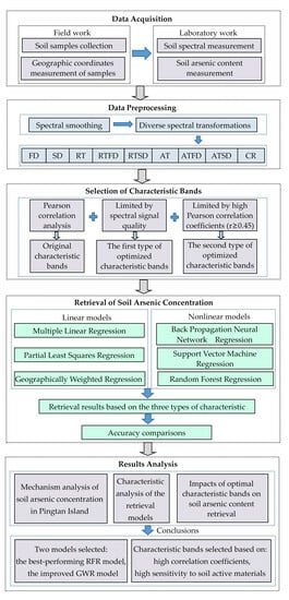
2. Materials and Methods

2.1. Study Area and Experimental Data

As shown in Figure 1, Pingtan Island is located southeast of Fuzhou City, bordered by the Taiwan Strait to the east and Changle and Fuqing across the Haitan Strait to the west, stretching 30 km from north to south and 19 km from east to west, with an area of 274.33 km² located between 25°15′–25°45′ north latitude and 119°32′–120°10′ east longitude. It is situated in the subtropical evergreen broad-leaved forest vegetation zone, characterized by low-level topography, with the central part slightly elevated. Dominated by sea-accumulated plains, the region enjoys a long summer and a short winter, with warm and humid climatic conditions. Furthermore, the area receives an average annual precipitation of 1172 mm, making it one of the less rainy areas in Fujian Province.

Based on various environmental factors, such as soil texture, land use and topographic characteristics in the study area, carefully selected sampling points were positioned to collect soil samples from late July to early August 2013. A meticulous five-point sampling method was employed to ensure the accuracy of samples and to avoid the effects of soil disturbance or transfer by some human activities. This method entailed sampling the central point along with four surrounding points located approximately 10 m apart, subsequently combining them to form a composite sample. Crucially, the geographical coordinates and type of features in each sampling point were recorded using a handheld Global Positioning System (GPS). Only surface soil located at a depth of 0–20 cm was collected from a total of 72 sampling points (Figure 1). To ensure the precision of the subsequent analyses, the soil samples were air-dried and crushed before being screened through a 100-mesh sieve. The resulting soil was then divided into two parts using the quarter method. One part was subjected to hyperspectral determination, and the other was analyzed for heavy metal arsenic content. The soil arsenic content was determined via inductively coupled plasma mass spectrometry (ICP-MS, Thermo Electron, Waltham, MA, USA). The following sections discuss the soil spectral measurements and pre-processing in detail.

The ASD FieldSpec4 spectroradiometer (Analytical Spectral Device, Boulder, CO, USA), which covers spectrum bands ranging from 350 to 2500 nm, was used to obtain soil spectral data. A halogen lamp with a band range of 350–2500 nm and a sampling interval of 1 nm was chosen as the exclusive light source in a darkroom to reduce the influence of foreign light. Further, to minimize scattered light caused by uneven surfaces, a pretreated 2 cm soil sample was placed on a black velvet cloth inside a glass culture vessel with a diameter of 10 cm, with its surface scraped flat. The light source was 30 cm away from the soil sample surface, and the zenith angle of the light source was set to 30°. The probe was placed 15 cm vertically above the surface of the soil sample, the field of view angle of the optical fiber probe was 5°, and the field of view was approximately 2.61 cm. The use of a standard whiteboard for calibration helped with obtaining absolute reflectivity. To decrease the error caused by measurement instability, each soil sample was tested ten times, and after removing the abnormal spectral curves, their average value was taken as the actual reflectance spectrum data of the soil sample.

To diminish interfering background noise and enhance the characteristics of the original spectral curve, it is imperative to smooth the spectral curve and transform the spectral data before the construction of a spectral retrieval model [21]. To attain this objective, the original spectrum was subjected to Savitzky–Golay smoothing to lessen the effects due to the different optical environments of the laboratory and the effects of sample grinding [22]. Moreover, low-order differential transformation of spectral data facilitates the removal of background drift and baseline interference while augmenting discernible information in the original data and emphasizing unapparent traits of the soil’s natural spectrum [23]. Continuum Removal (CR) is also employed to eliminate the background signals and extract feature bands. Therefore, in this study, the smoothed spectral data were subjected to an array of transformations, including first-order differential (FD), second-order differential (SD), reciprocal (RT), reciprocal first-order differential (RTFD), penultimate second-order differential (RTSD), reciprocal logarithmic (AT), reciprocal logarithmic first-order differential (ATFD), reciprocal logarithmic second-order differential (ATSD) and continuum removal (CR). The correlation between the arsenic concentration, as measured, and the above-mentioned spectral transformation data was tested to identify the band exhibiting the highest correlation.

2.2. Retrieval Methods of Soil Arsenic Concentration

A

Multiple Linear Regression Model (MLR)

Multiple Linear Regression is the expression of a linear relationship between a dependent variable and a combination of multiple independent variables. The MLR model is a classical statistical analysis method based on the least squares method, and its regression equation is [24]

$$y={\beta }_0+{\beta }_1{x}_1+{\beta }_2{x}_2+\cdots +{\beta }_n{x}_n+\epsilon$$

(1)

where y is the dependent variable, x is the independent variable, β_i (i = 0, 1, 2, …, k) is the regression coefficient, which represents the random error, and k represents the number of independent variables. The measured concentration of arsenic was used as the dependent variable of the modeling sample, and the characteristic spectrum was used as the independent variable to establish the MLR model.

B

Partial Least Squares Regression Model (PLSR)

Partial Least Squares Regression, proposed by Wold et al. [25], is a linear regression modeling method of multiple dependent variables to multiple independent variables. It combines the advantages of principal component analysis and linear regression models and is more conducive to distinguishing spectral information and noise [26]. Its modeling principle is to establish the spectral matrix X of m × n, and the heavy metal content detection matrix Y of n × l, where m is the number of spectral bands, n is the number of samples, and l is the heavy metal type.

The method decomposes X and Y with the following formula [25]:

$$\begin{gathered} X=T{P}^T+E \\ Y=U{Q}^T+F \end{gathered}$$

(2)

where U and T are the score matrix, P and Q are the loads, and E and F are the residual matrices of PLSR. For the linear regression between U and T, with B as the relationship coefficient matrix, U = TB is used, and the formula for predicting the heavy metal content is

$$\begin{array}{c}{Y}_{predicted}=T_{calculated}BQ\hfill \\ =X_{measured}{P}^{T}BQ\hfill \end{array}$$

(3)

where Y_predicted represents the predicted value of the heavy metal content, and X_measured is the independent variable, which is the spectral matrix of the characteristic variables.

C

Geographically Weighted Regression Model (GWR)

The Geographically Weighted Regression model is a nonparametric local spatial regression analysis method initially proposed by geographers at Newcastle University in the United Kingdom. The aim of this method is to model spatial variation between independent and dependent variables of different spatial subregions [27]. The GWR model is an extension of the ordinary least squares regression model, which explains the spatial relationship between the dependent and independent variables. This technique is widely used to explore non-stationary spatial relationships and has yielded excellent results in predicting soil properties [28]. Because the relationship between soil heavy metal content and spectral characteristics is affected by spatial heterogeneity, this paper uses the GWR model to add the coordinate data of the sampling points and embed them into the regression equation as spatial data, as follows [27]:

$$y_i={\beta }_0\left(u_i,v_i\right)+{\displaystyle \sum }_{k=1}^p{\beta }_k\left(u_i,v_i\right)x_{ik}+{\epsilon }_i i=1,2, \dots ,n$$

(4)

In the above formula, the coordinate of the sampling point i and the k_th regression parameter on the sampling point i are functions of the geographic location obtained using the weight function method in the estimation process. Calculating the spatial weight function is the core part of the GWR model, and this paper selects the spatial weight matrix of the Gauss function method to calculate the model. Its calculation formula is [28]

$$w_{ij}=exp\left(-{\left(d_{ij}/b\right)}^2\right)$$

(5)

where b represents a non-negative attenuation parameter that characterizes the functional relationship between the weight and the distance. This parameter effectively determines the bandwidth, whereby a larger bandwidth corresponds to a slower decay of weight with increasing distance. Conversely, a smaller bandwidth results in a faster decay of weight. The basic idea of the Gauss function method is to express the relationship between weight and distance by selecting a continuous monotonically decreasing function with good universality.

D

Back Propagation Neural Network Model (BP)

A neural network, the most prevalent example being the BP neural network, is a mathematical model that mimics the synaptic structure of human neurons and facilitates the processing of information. The framework operates based on the error back propagation algorithm, involving forward propagation of the input signal and subsequent backward propagation of the error [29]. Its basic architecture is divided into the input, hidden and output layers. The input layer relays data to the neurons and generates output information through signal propagation. The error is calculated against the expected output and is forwarded to the corresponding neuron in the hidden layer through back propagation, triggering the adjustment of weights and threshold levels according to the aforementioned error. The iterative process thus optimizes the neural network’s predictive accuracy until it reliably approximates the measured value [30]. The soil spectral data are usually used as the input layer, the hidden layer is the algorithm of the model, and the output layer is the heavy metal concentration. In this paper, the number of nodes in the input layer was set to 10, the number of nodes in the output layer was set to 1, tansig was used as the activation function of the model, and the back propagation algorithm was used to train and determine that the optimal number of nodes in the hidden layer is 12.

E

Support Vector Machine Regression Model (SVR)

Support Vector Machine is a machine learning method based on the Vapnik–Chervonenkis dimension theory and structural risk minimization proposed by Vapnik [31]. It is developed from the optimal classification surface under the condition of linear separability, which can handle small samples and nonlinear and high-dimensional problems, and it can overcome local optimal solution problems in neural networks [32,33]. The basic principle is to use a nonlinear map p to convert low-dimensional data into high-dimensional or multidimensional data, and through the transformation of data dimensions, low-dimensional nonlinear problems can be transformed into high-dimensional linear problems [34]. The Support Vector Machine Regression model consists of two parts: linear regression and nonlinear regression. In this experiment, the cross-validation method was used to help find the model’s best c (penalty coefficient) parameter and g (kernel function parameter gamma) parameter. The radial basis function was selected as the kernel function, with the value of the loss function p set to 0.4. The model was trained, and the regression predictions were made using the svmtrain function and the svmpredict function in the MATLAB R2021a environment.

F

Random Forest Regression Model (RFR)

The fundamental principle of Random Forest lies in the utilization of random classification technology, which involves the use of Bootstrap aggregation (Bagging) to devise a group of nodes comprising weak classifiers. Through this process, the data are distributed into various decision trees, and the best classification results are determined through voting. This method can solve both classification and regression problems by employing binary data segmentation algorithms [35,36]. Concerning classification problems, the Gini coefficient is used to segment the data. Regarding regression problems, weighted averages are used for training samples, which enables the training of a large number of decision trees without the need for pruning. The final outcome is determined through voting. In this experiment, we utilized the TreeBagger function within the MATLAB R2021a environment to train the model. Specifically, we configured it as a regression tree model with instructions for regression analysis. The optimal number of leaf nodes and the optimal number of trees were determined to be 3 and 200, respectively, and the final model training time was 2.33 s. Consequently, the Random Forest algorithm demonstrates a swift training speed, can process high-dimensional data without requiring feature selection, possesses strong dataset adaptability and performs well in the hyperspectral retrieval of soil heavy metals due to its simple implementation, high precision and strong overfitting resistance.

3. Results

3.1. Statistical Analysis of Soil Arsenic Concentration in Pingtan Island

Table 1. Soil arsenic (As) background value in China and Fujian Province.

Element	Standard Value in China (mg/kg)				Background Value in Fujian Province (mg/kg)
	Type	PH <6.5	PH 6.5–7.5	PH >7.5
As	dry land	30	30	25	5.87
	paddy field	40	25	20

shows arsenic content values from the environmental quality standard of China [37] and the arsenic background value of soil in Fujian province of China [25]. Through the statistics of the basic characteristics of arsenic concentrations in the soil of 72 samples in the study area (

Table 2. Statistical information for soil arsenic (As) concentration in the study area (unit: mg/kg).

Element	Min	Max	Mean	SD	Skewness	Kurtosis	CV
As	6.33	114.81	43.43	20.43	0.64	1.18	47

), the total arsenic concentration of the sample varied between 6.33 and 114.81 mg/kg. From the perspective of heavy metal contamination, the average value of arsenic was 43.43 mg/kg, which was higher than the national soil environmental quality three-level standards, indicating that the study area was seriously polluted by arsenic. Even when referring to the new national soil environmental quality standard [38], a soft standard distributed in 2018, arsenic values of 42/72 soil samples exceeded 40 mg/kg—the highest risk screening values for the soil contamination of agricultural land. From the spatial distribution of heavy metals, the coefficient of variation of arsenic was 47%, signifying significant variations. Such a coefficient of variation reflects the influence of human activities on arsenic content within the region. Therefore, the statistical results indicate that the arsenic concentration in the study area was non-uniformly distributed in the soil, with an evident spatial heterogeneity. This inconsistency may be attributed to the substantial influence of local anthropogenic activities.

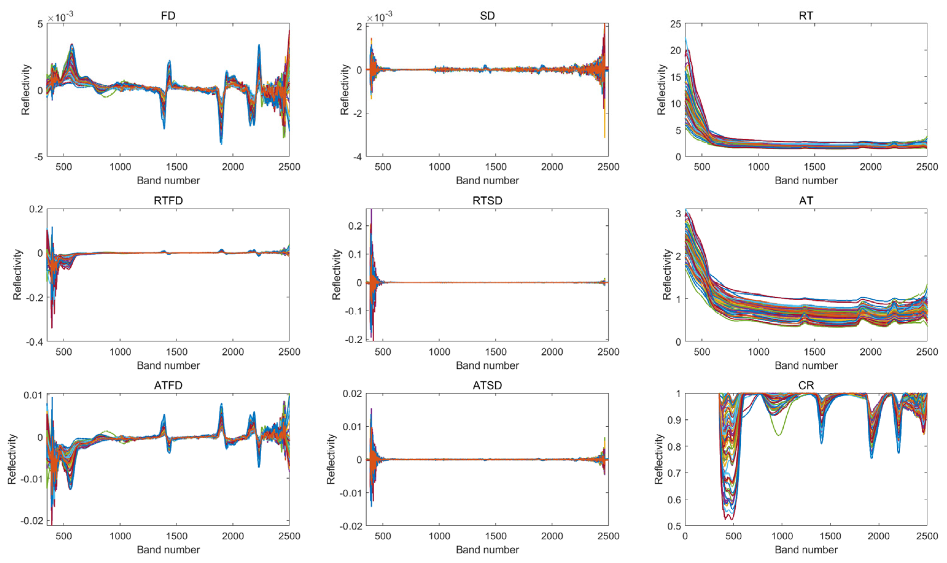
3.2. Spectral Characteristics Analysis of Soil Samples in Pingtan Island

The content of heavy metals in soil is influenced by the adsorption and fixation of these metals onto soil components, such as organic matter, iron oxides and clay minerals, which are known as soil spectroscopic active substances. The connection between heavy metals and these substances forms the basis for estimating heavy metal content through soil reflectance spectroscopy. Figure 2 illustrates the reflectance spectrum of soil samples collected from Pingtan Island. All soil samples exhibited a similar trend of changes in spectral curves. The reflectivity in the visible light band was low, and spectral reflectance increased with wavelength. In the near-infrared band, the overall spectral curve flattened. However, a low-quality region, represented by the red box in the spectral range of approximately 2300 nm–2500 nm, possessed irregularities and frequent crossings that were most pronounced from approximately 2400 nm to 2500 nm. This issue could potentially impact the selection of effective characteristic bands of the soil arsenic concentration with the original reflectance data and their diverse transformations. The spectral curve showed reflection peaks of organic matter near the 600 nm and 800 nm bands, along with three pronounced water absorption bands near the 1400 nm, 1900 nm and 2200 nm bands that were influenced by silicate minerals and clay minerals in the soil. Furthermore, Figure 3 presents the spectral curves after diverse data transformations. The spectral curves of the FD and ATFD transformations fluctuated considerably. The RT and AT transformations declined rapidly from the starting band before, showing a trend of slowing down around 600 nm. The changes in reflectance after RTFD, RTSD, ATSD and SD conversion mainly appeared before 500 nm and after 2200 nm. After CR transformation, the spectral curve was normalized between 0 and 1, and the absorption valley mainly appeared around 500 nm, 1000 nm, 1400 nm, 1900 nm and 2200 nm.

To explore the relationship between different spectral indexes and arsenic concentration, the arsenic concentration and various spectral transformations were analyzed with Pearson’s correlation.

Table 3. Original characteristic bands of arsenic concentration with spectral indicators.

Spectral Indicator	Original Characteristic Band /nm	Maximum Pearson’s Correlation Coefficient
SR	2440	0.5264 **
FD	478	0.4460 **
SD	1398	−0.4414 **
RT	2441	−0.5151 **
RTFD	1349	−0.4947 **
RTSD	1423	0.5145 **
AT	2440	−0.5224 **
ATFD	1349	−0.4622 **
ATSD	1423	0.4594 **
CR	2152	0.3882 **

** denotes statistical significance at the 0.01 level (two-tailed).

shows the maximum correlation coefficient and its corresponding original characteristic bands, where ‘-’ indicates that the reflectance spectrum of the band is negatively correlated with the concentration of heavy metals; otherwise, it is represented as a positive correlation.

The analysis presented in Table 3 demonstrates a positive correlation between the arsenic concentration and SR, FD, RTSD, ATSD and CR regarding smoothed spectral reflectance. In contrast, there is a negative correlation between arsenic concentration and SD, RT, RTFD, AT and ATFD. Notably, the highest correlating bands for all transformations (except for FD) were found within the near-infrared spectrum. The highest correlation coefficient found in the CR was below 0.4 (p < 0.01), and all other transformations yielded correlation coefficients exceeding 0.4 (p < 0.01).

Based on the spectral analysis conducted above, it was observed that several characteristic bands in the vicinity of 2500 nm in Table 3 may be contaminated by excessive noise; this noise could hinder the effective use of the information within these bands for enhancing retrieval accuracy. To address this, the optimal selection of characteristic bands was examined and tested based on two criteria: statistical one (using Pearson’s correlation coefficients) and physical spectral quality (including sensitivity to soil active materials such as soil organic matter, clay minerals and iron oxides).

Table 4. First type of optimal selection of characteristic bands with spectral indicators of SR/RT/AT.

Spectral Indicator	Optimal Characteristic Band/nm	Second-Highest Correlation Coefficient
SR	2212	0.4986 **
RT	2390	−0.4954 **
AT	2384	−0.4930 **

** denotes statistical significance at the 0.01 level (two-tailed).

and

Table 5. Second type of optimal selection of characteristic bands with spectral indicators of SR/RT/AT.

Spectral Indicator	Optimal Characteristic Band/nm	High Correlation Coefficient
SR	2212	0.4986 **
RT	2212	−0.4839 **
AT	2212	−0.4925 **

** denotes statistical significance at the 0.01 level (two-tailed).

present the optimal characteristic bands for arsenic concentration, taking into account the spectral indicators of SR/RT/AT. The first type of optimal selection, as shown in Table 4, was made under the criteria of the second-highest Pearson’s correlation coefficients and higher-quality spectral data. Moreover, the second type of optimal selection, as shown in Table 5, was made under the criteria of high Pearson’s correlation coefficients (abs(Pearson’s correlation coefficient) ≥ 0.45) combined with sensitivity to soil active materials.

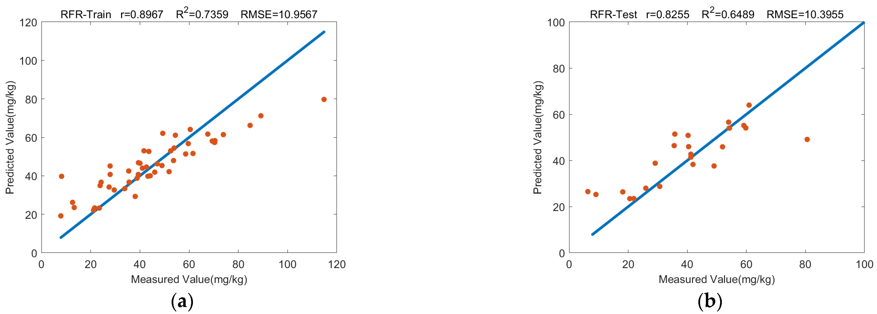
3.3. Retrieval Models’ Construction of Soil Arsenic Concentration in Pingtan Island

(1)

Based on original characteristic bands

Through Pearson’s correlation analysis between arsenic concentration and soil spectra, spectral bands with high correlations were identified. Linear models (MLR, PLSR and GWR) and nonlinear models (BP, SVR and RFR) were used for retrieval analysis, using a total of 72 samples. The training set comprised 70% of the sample data, and the validation set comprised 30%. The correlation coefficient (r), the coefficient of determination (R²) and the root-mean-square error (RMSE) were used to evaluate the retrieval performance of the model (

Table 6. Retrieval results based on original characteristic bands in Table 3.

Model	Training Data			Validation Data
	r	R2	RMSE (mg/kg)	r	R2	RMSE (mg/kg)
MLR	0.6400 **	0.4097	16.1806	0.6487 *	0.4058	15.3761
PLSR	0.6720 **	0.4516	16.1028	0.6940 **	0.4738	11.8161
GWR	0.7461 **	0.5541	13.8338	0.7441 **	0.5420	13.0101
BP	0.7003 **	0.4895	15.1688	0.7358 **	0.5407	8.0496
SVR	0.6477 **	0.4163	15.5690	0.6389 *	0.3899	15.6473
RFR	0.8967 **	0.7359	10.9567	0.8255 **	0.6489	10.3955

** denotes statistical significance at the 0.01 level (two-tailed), * denotes statistical significance at the 0.05 level (one-tailed).

). The best regression model was determined according to the larger values of r and R², the smaller RMSE value and the close scatter distribution of the training data and the validation data, indicating optimal model performance.

Upon comparing the accuracy of the linear models (MLR, PLSR and GWR), it was discovered that PLSR outperformed MLR for both the training and validation data, with a higher correlation coefficient r and coefficient of determination R² and a smaller RMSE. Further analysis revealed that, although GWR had a slightly higher RMSE in its validation data than that of PLSR, it still demonstrated superior accuracy in other performance indicators, with a correlation coefficient r exceeding 0.7 and a coefficient of determination R² greater than 0.5 (Figure 4). Hence, the linear models can be ranked in terms of accuracy as follows: GWR > PLSR > MLR.

In the realm of nonlinear modeling, the R² values for the SVR and BP models clocked in at approximately 0.4 and 0.5, respectively. On the other hand, the R² of the RFR model consistently exceeded 0.6 (Figure 5), a figure that far surpasses the other two models. Even though the RFR’s validation data displayed a slightly larger RMSE when compared to the BP model, its r value stands at a significant 0.8, and the RMSE value was less than 15 mg/kg. Therefore, when looking at accuracy in the nonlinear model, RFR, BP and SVR can be successively ranked as RFR > BP > SVR.

The accuracy of the six prediction models for arsenic concentration in this study area varied, and their performance can be ranked as follows: RFR > GWR > BP > PLSR > SVR > MLR, for the correlation coefficient r value of the training data, and RFR > GWR > BP > PLSR > MLR > SVR, for the correlation coefficient r value of the validation data. Therefore, the RFR model exhibited the highest accuracy in both scenarios, followed by the GWR model. The ranking of the other models differed slightly between the training and validation data sets. Specifically, the RFR model boasted the highest degree of accuracy, with the r, R² and RMSE of the validation data being 0.8255, 0.6489 and 10.3955, respectively. The accuracy of the GWR model was second to that of RF, and the r, R² and RMSE of the validation data were 0.7441, 0.5420 and 13.0101, respectively. Experimental outcomes underlined the RFR’s excellent retrieval performance in this study for the nonlinear model, emphasizing that the concentration and spectrum of the arsenic concentration in the soil was not a simple linear relationship, which may be affected by soil type and climatic factors. Thus, the retrieval accuracy of the simple linear models was limited. Moreover, the GWR model in the linear model also showed an excellent retrieval performance in this experiment as the spatial coordinate information of the sample points was integrated into the construction of the GWR model, which thoroughly considered the spatial non-stationarity between the soil arsenic concentration and the reflectance spectrum. This spatial heterogeneity is often ignored in most models. Although the accuracy of the GWR model still has a greater improvement compared to the RFR model, the retrieval performance of the model further demonstrated the existence of spatial heterogeneity between the arsenic concentration and the spectrum in the study area, allowing for the construction of a more precise and stable retrieval model.

(2)

Based on the first type of optimal characteristic bands

Similar to the process described earlier, the correlation coefficient, coefficient of determination and root-mean-square error were calculated to evaluate the retrieval models using the optimal characteristic bands. These evaluations were conducted based on the retrieval results with the first type of optimal characteristic bands, considering the two criteria of the second-highest Pearson’s correlation coefficients and higher-quality spectral data. The results of these evaluations can be found in

Table 7. Retrieval results based on the characteristic bands in Table 3 and Table 4.

Model	Training Data			Validation Data
	r	R2	RMSE (mg/kg)	r	R2	RMSE (mg/kg)
MLR	0.6500 **	0.4224	15.5881	0.7145 **	0.4287	15.7926
PLSR	0.66711 **	0.4504	14.8022	0.6842 **	0.4671	15.0733
GWR	0.7392 **	0.5407	12.9545	0.7982 **	0.6286	13.5795
BP	0.7186 **	0.4682	12.6433	0.6759 **	0.4426	12.7430
SVR	0.6597 **	0.4233	15.7397	0.6333 *	0.3856	15.0533
RFR	0.8894 **	0.7347	10.9802	0.8004 **	0.6151	10.8847

** denotes statistical significance at the 0.01 level (two-tailed), * denotes statistical significance at the 0.05 level (one-tailed).

.

From Table 3 and Table 4 and Table 6 and Table 7, the following findings can be derived: (1) When comparing the retrieval results based on both the original characteristic bands and the optimal ones, the RFR and GWR models consistently demonstrated the best and second-best performance, respectively. (2) However, there were changes in the accuracy rankings. Specifically, when considering the correlation coefficient (r) values for the validation data, the rankings changed from the original order of RFR > GWR > BP > PLSR > MLR > SVR to the optimal order of RFR > GWR > MLR > PLSR > BP > SVR. In the optimal scenario, the ranking positions of linear models increased from the r values of the validation data.

Additionally, the following observations can be made: (1) The linear models (MLR, PLSR and GWR) exhibited greater sensitivity toward the optimal characteristic bands. The accuracy of both the MLR and GWR models improved significantly. Specifically, for the MLR model, the r value of the validation data increased from 0.6487 to 0.7145, showing good statistical significance. Similarly, for the GWR model, the r value of the validation data increased from 0.7441 to 0.7982. (2) However, for the nonlinear models (SVR, BP and RFR), the r metric generally decreased, except for the r value of the training data for the BP and SVR models. Overall, the use of optimal characteristic bands resulted in decreased performance for these nonlinear models in terms of retrieval results.

In summary, the linear models (MLR, PLSR and GWR) demonstrated improved sensitivity to the optimal characteristic bands, resulting in enhanced accuracy. On the other hand, the nonlinear models (SVR, BP, and RFR) evinced weakened efficacy in utilizing the optimal characteristic bands, except for the r value of the training data for the BP and SVR models.

(3)

Based on the second type of optimal characteristic bands

Similar to the previous analysis, the correlation coefficient, coefficient of determination and root-mean-square error were calculated to evaluate the retrieval models using the optimal characteristic bands. This evaluation was conducted based on the retrieval results with the second type of optimal characteristic bands, considering the criteria of high Pearson’s correlation coefficients (abs(Pearson’s correlation coefficient) ≥ 0.45) combined with sensitivity to soil active materials. The results of this evaluation can be found in

Table 8. Retrieval results based on the characteristic bands in Table 3 and Table 5.

Model	Training Data			Validation Data
	r	R2	RMSE (mg/kg)	r	R2	RMSE (mg/kg)
MLR	0.6493 **	0.4215	16.2586	0.6954 **	0.4665	14.0281
PLSR	0.6777 **	0.4593	14.6014	0.7159 **	0.4912	15.0675
GWR	0.7301 **	0.5285	13.1248	0.8052 **	0.6461	13.2556
BP	0.6562 **	0.4105	14.9417	0.7331 **	0.5240	10.0690
SVR	0.6635 **	0.4352	15.7681	0.6165 *	0.3640	14.8183
RFR	0.8996 **	0.7406	10.8576	0.7776 **	0.5878	11.2641

** denotes statistical significance at the 0.01 level (two-tailed), * denotes statistical significance at the 0.05 level (one-tailed).

.

Based on Table 3, Table 4, Table 7 and Table 8, the following observations can be made: (1) When comparing the retrieval results using both the original characteristic bands and the optimal ones, the RFR and GWR models generally maintained their positions as the best and second-best performers, respectively. (2) However, there were changes in the accuracy rankings. Specifically, when considering the correlation coefficient (r) values for the training data, the rankings changed from the original order of RFR > GWR > BP > PLSR > SVR > MLR to the optimal order of RFR > GWR > PLSR > SVR > BP > MLR. Similarly, when considering the correlation coefficient (r) values for the validation data, the rankings changed from the original order of RFR > GWR > BP > PLSR > MLR > SVR to the optimal order of GWR > RFR > BP > PLSR > MLR > SVR. In the optimal scenario, the ranking positions of linear models increased from the r values of both training and validation data. Specifically, the GWR model achieved the highest r value for validation data.

The following additional observations can be made: (1) The linear models (MLR, PLSR and GWR) appeared to be more sensitive to the optimal characteristic bands, and all of them showed improvements in the r metric, except for the r value of the training data for the GWR model. Specifically, for the MLR model, the r value of the validation data increased from 0.6487 to 0.6954 with good statistical significance. Similarly, for the GWR model, the r value of the validation data increased from 0.7441 to 0.8052, representing the highest r value among all models for the validation data. (2) However, for the nonlinear models (SVR, BP and RFR), the performance varied, with some r values for both the training and validation data increasing and others decreasing. Overall, the retrieval results based on both the original characteristic bands and the optimal ones presented a minor decline in performance for these nonlinear models.

In summary, the linear models (MLR, PLSR and GWR) exhibited greater sensitivity to the optimal characteristic bands, resulting in improved accuracy for most metrics. Conversely, the performance of the nonlinear models (SVR, BP and RFR) showed mixed results, with some metrics improving and others declining when using the optimal characteristic bands.

4. Discussion

4.1. Mechanism Analysis of Soil Arsenic Concentration in Pingtan Island

Research has shown that iron oxides have an impact on the spectral quantitative retrieval of soil heavy metals [39]. With an increase in iron oxide content or a higher ratio of iron oxide content to organic matter content, the stability and predictive ability of the retrieval model weaken, leading to the formation of absorption bands around 500 nm and 950 nm due to iron oxides. In Figure 2, a weak absorption band is presented at around 500 nm, and a distinct absorption band is visible at around 950 nm, suggesting the potential presence of increased iron oxide content within the study area [40,41]. Table 3 also confirms the presence of characteristic bands at around 500 nm in the soil spectra of the study area, which highlights the potential noteworthy influence of iron oxides on the concentration of arsenic. Iron oxide minerals are also the most important source of soil arsenic [42,43], which is a geological factor contributing to the overall higher arsenic content in the soil of Pingtan Island. Furthermore, previous studies have shown that the absorption features of soil clay minerals are located at around 1400 nm [44,45,46], 1900 nm [45,46] and 2200 nm [44,47,48,49]. For field spectrometry and image spectroscopy, 1400 nm and 1900 nm were affected by strong atmospheric water vapor absorption, so the inversion modeling primarily utilized the absorption feature at 2200 nm. The laboratory spectra measured in this study indicated prominent absorption peaks at 1400 nm, 1900 nm and 2200 nm, as shown in Figure 2. Table 3, Table 4 and Table 5 also confirmed the presence of characteristic bands at around 1400 nm and 2200 nm in the soil spectra of the study area, indicating the possible significant feedback of clay minerals on arsenic content in Pingtan Island’s soil. Clay minerals are also an important source of soil arsenic [50]. Pingtan Island hosts 15 kinds of minerals (including sub-minerals), such as iron, copper, tungsten, molybdenum, quartz sand, alunite and decorative stones. Of particular note are the abundant reserves of casting sand, standard cement sand, glass sand, gabbro for decoration and granite for decoration, which were included in the list of mineral resources in Fujian Province in 2015 (https://www.pingtan.gov.cn/jhtml/ct/ct_9241_124464 (accessed on 1 September 2023)). Therefore, mining these mineral resources may provide an important source for the accumulation of arsenic in soil. Moreover, as a relatively closed land area with limited space, Pingtan Island’s topography and geomorphology are not conducive to the migration, diffusion and dilution of soil arsenic, further intensifying the accumulation and pollution of arsenic in the soil.

In addition, the spectral response range of soil organic matter predominantly occurs within the range of 400 nm and 1100 nm, with the most significant changes happening between 600 nm and 800 nm [51,52]. Based on the soil spectral curves shown in Figure 1 and the characteristic bands of the soil arsenic concentration presented in Table 3, Table 4 and Table 5, it was observed that there were no significant peaks or strong correlations that could indicate a direct relationship between the soil organic matter and soil arsenic content. However, the characteristic band at 1349 nm with the RTFD indicator shows the potential influence of organic matter [53]. Overall, the impact of soil organic matter on soil arsenic accumulation in the study area was found to be limited. Hence, it is suggested that soil organic matter may not be a major factor influencing the accumulation of arsenic in the study area. This analysis is consistent with the objective condition of relatively low organic matter content in the soil of Pingtan Island (https://www.pingtan.gov.cn/jhtml/ct/ct_2948_97751 (accessed on 1 September 2023)).

It should be noted that the characteristic bands of soil spectra in Pingtan Island may slightly differ from those cited in the literature due to variations in soil texture classes across different regions, differences in spectral data acquisition and variations in spectral pre-processing methods. However, these differences do not significantly impact the overall reliability of the analysis.

4.2. Assessment of Ground-Based Hyperspectral Retrieval of Soil Arsenic Concentration in the Study

The geochemical data obtained from investigating soil heavy metals have proven to be precise, making it a reliable basis for ecological risk assessments in various studies [54,55,56,57,58]. However, these data are generally discrete, sparse and relevantly stationary, which cannot satisfy the frequent and rapid monitoring requirement for a wide area. Consequently, using hyperspectral remote sensing to retrieve soil heavy metal content presents a unique advantage for rapid and dynamic observations across a wide area. Although it may be challenging to directly retrieve soil heavy metal content from remote sensing imagery due to various factors, including atmospheric effects and sensor limitations, ground-based hyperspectral retrieval studies can provide significant theoretical and technical support for satellite-based studies. Multi-model retrieval studies of soil arsenic concentrations with ground-based hyperspectral data are particularly important and were explored in this paper. The pre-processing of soil spectra before the selection of characteristic bands helps eliminate background noise to create more prominent reflection peaks and absorption valleys, improving the accuracy of hyperspectral modeling. Studies have shown that spectral differential technology could effectively eliminate curves’ drift phenomenon and linear background interference, thus facilitating the discovery of sensitive spectral characteristic parameters among different heavy metals. Moreover, the reciprocal logarithmic variation in the spectrum helped attenuate random effects, such as those caused by topography and lighting [59]. This study employed nine transformation forms to transform the data: first-order differentiation, second-order differentiation, reciprocal, reciprocal first-order differentiation, reciprocal logarithmic first-order differentiation, reciprocal logarithmic second-order differentiation and continuum removal. Subsequently, the use of Pearson’s correlation analysis helped screen out bands with significant correlations as characteristic bands for the retrieval modeling process, minimizing high-dimensional data redundancy and mitigating data collinearity to a certain extent. However, this method also possessed limitations, as the correlation between the spectral data and soil heavy metal content did not significantly improve in this study after transformation, which differed from the results of Teng et al. [60]. Furthermore, filtering feature bands posed the potential risk of removing some bands with rich feature information, ultimately affecting the accuracy of the subsequent model’s establishment.

Due to the abundance and diversity of soil types, modeling heavy metal content using a single method proves to be challenging. Thus, six modeling methods based on linear and nonlinear models were selected in this study to estimate the arsenic concentration. The model exhibiting the highest precision was chosen as the optimal retrieval model in the study area. Numerous studies have consistently demonstrated that models based on nonlinear relationships tend to exhibit higher accuracy compared to linear relationship models. For instance, Gholizadeh et al. [61] conducted a comparative analysis of two models using soil samples from a large brown coal mining dumpsite in the Czech Republic. Their findings indicate that the Support Vector Regression (SVR) model outperforms the Partial Least Squares Regression (PLSR) model in terms of accuracy. However, in this study, the precision of linear models such as MLR, PLSR and GWR was superior to that of nonlinear models such as SVR in validation data, and the accuracy of the GWR model was greater than that of the BP model. This result may be due to the problem of achieving a locally optimal solution when performing parameter optimization while using machine learning methods in modeling. As such, to enhance the modeling precision of BP and SVR, it is necessary to further optimize algorithms to attain an optimal global solution. For example, Shi et al. [62] used the LASSO (least absolute shrinkage and selection operator) algorithm and GA (genetic algorithm) to optimize BP, which greatly improved the estimation accuracy and generalization ability of the model.

The accuracy of retrieving heavy metal content using the nonlinear model RFR in this study far surpassed that of other models. The reason is that the relationship between the reflectance spectrum of the soil and the heavy metal content is not ideally linear. For example, the spectral characteristics of heavy metals do not consistently increase with a higher concentration. Furthermore, the characteristic bands of heavy metals at the same concentration differ among different soil types due to the influence of organic matter and other components [18]. Therefore, employing nonlinear models can overcome the problems of overfitting and insufficient explanatory properties in linear models, resulting in greater retrieval accuracy. In addition, when there is significant spatial heterogeneity between the soil heavy metal content and the reflectance spectrum, models such as MLR, PLSR, BP, SVR and RFR do not account for spatial variables, which subsequently affects retrieval accuracy. Conversely, the GWR model incorporates spatial coordinate data into the modeling process, fully considering the spatial non-stationarity between the soil heavy metal content and the reflectance spectrum [63]. That is why the GWR model in this study also demonstrated good retrieval performance, with accuracy that was second only to the RFR model, further underscoring the presence of spatial heterogeneity between the soil arsenic concentration and the reflectance spectrum in the study area.

4.3. Impacts of Optimal Characteristic Bands on Soil Arsenic Content Retrieval

The approach of selecting the optimal Pearson’s correlation coefficient coupled with a spectrum that is highly sensitive to the active constituents within the soil has a favorable impact on constructing prediction models for soil-borne heavy metals. Prior studies, such as that carried out by Lu et al. [64], have also verified the feasibility of this method. Their research, focusing on heavy metal concentrations in karstic regions, demonstrated that the utilization of spectral response bands linked to clay minerals and organic matter was instrumental in enhancing the accuracy and stability of the prediction models. Similarly, Lin et al. [65] identified a specific spectral band with an arsenic content correlation coefficient surpassing 0.5 as being particularly sensitive when establishing heavy metal prediction models. This band was associated with the active constituents of the soil spectrum (specifically those at 500 nm and 800 nm). Nonetheless, the extent to which this band selection method affects the precision of diverse heavy metal models remains unexplained; thus, our study offered a more profound analysis.

For linear models (MLR, PLSR and GWR), the relationship between characteristic bands and soil heavy metals is relatively simple. This means that any variations in the characteristic bands for SR/RT/AT are linearly propagated to the retrieval models. As a result, the overall training and validation results showed a direct variation for these linear models. Although the optimal characteristic spectra may not align with the highest Pearson’s correlation coefficients, the overall improvements for the linear models highlighted in Section 3.3 were significant. This improvement demonstrates that the selected characteristic spectra were effective, and the selection strategy was reasonable, particularly considering the two criteria of a high Pearson’s correlation coefficient (e.g., abs(Pearson’s correlation coefficient) ≥ 0.45) and sensitivity to soil active materials (soil organic matter, clay minerals and iron oxides).

On the other hand, regarding nonlinear models, two points can be observed: (1) The optimal characteristic bands with SR/RT/AT may not directly affect the accuracy improvement of the nonlinear models, even though the results obtained based on optimal characteristic bands indicate a slightly inferior accuracy. (2) When comparing the retrieval results based on original characteristic bands and optimal ones, the RFR model overall demonstrated the highest accuracy. These observations further emphasize that the relationship between characteristic bands and soil heavy metals is complex and nonlinear.

Consequently, the optimal selection of characteristic bands, determined based on the two criteria of a high Pearson’s correlation coefficient and sensitivity to soil active materials, provide two effective retrieval models: the best RFR model and the improved GWR model.

4.4. Limitations of This Study and Outlook for Future Studies

Indeed, there are still some unresolved issues in this study. The following points highlight these concerns:

• Machine learning methods lack clear physical meanings, which can lead to less stable and robust retrieval models. To address this, it should be considered that machine learning methods can achieve better retrieval performance when sufficient geochemical survey data are available. Additionally, considering the advantages of the GWR model, traditional machine learning models can be improved by incorporating spatial characteristics.
• The optimal selection of characteristic bands with SR/RT/AT transformation spectra was performed manually in this study. To enhance the process, future research can explore automatic selection methods that adhere to the criteria of high Pearson’s correlation coefficients (e.g., abs(Pearson’s correlation coefficient) ≥ 0.45) and sensitivity to soil active materials (e.g., soil organic matter, clay minerals and iron oxides). Notably, noticeable absorption peaks are observed at approximately 950 nm and 1900 nm in Figure 1, corresponding to the sensitive spectral ranges of soil active materials. However, these characteristic bands were not utilized in soil arsenic retrieval. Incorporating them has the potential to further improve the retrieval accuracy of soil arsenic concentrations.

The transition from ground-based hyperspectral retrieval to satellite-based retrieval poses different challenges and issues, such as the robustness of characteristic bands and the universal availability of optimal models. Therefore, it is crucial to consider the comprehensive use of both ground-based and satellite-based characteristic bands to address these challenges effectively [39].

5. Conclusions

Our findings from this study can be summarized as follows:

• Using both the original characteristic bands and the optimal ones, the RFR model exhibited the best performance. This suggests that the relationship between the soil arsenic concentration and its spectral variables is complex and nonlinear, influenced by various factors in the landscape. The GWR model also showed excellent performance as the second-best model, considering the spatial non-stationarity and heterogeneity of the relationship between the arsenic concentration and spectral variables. This highlights the importance of considering spatial characteristics in geospatial studies and indicates the potential for improving traditional machine learning modeling.
• When evaluating the accuracy rankings of the retrieval models based on optimal characteristic bands, the RFR model retained its position as the best-performing model. Although there was only a slight improvement in the r value of the training data, the accuracy of the linear models (MLR, PLSR and GWR) saw significant enhancements, particularly for the GWR model, which achieved the highest r value for the validation data. This demonstrates that the optimal characteristic bands, selected based on the two criteria of a high Pearson’s correlation coefficient and sensitivity to soil active materials, successfully addressed the issues of uncertainty and low quality in characteristic band selection based on Pearson’s correlation coefficients. Consequently, this study generated two effective retrieval models: the best-performing RFR model and the improved GWR model.

For Pingtan Island, the dynamic monitoring of soil arsenic content is crucial. Research provides theoretical and technical support for the monitoring and contamination evaluation of soil arsenic concentrations using satellite-based spectroscopy in relatively independent island towns with dense populations, such as Pingtan Island, both in China and worldwide.

References

1. Li, Z.Y.; Ma, Z.W.; Tsering Jan, V.D.K.; Yuan, Z.W.; Huang, L. A review of soil heavy metal pollution from mines in China: Pollution and health risk assessment. Sci. Total Environ. 2014, 468–469, 843–853. [Google Scholar] [CrossRef] [PubMed]
2. Rinklebe, J.; Antoniadis, V.; Shaheen, S.M.; Rosche, O.; Altermann, M. Health risk assessment of potentially toxic elements in soils along the Central Elbe River, Germany. Environ. Int. 2019, 126, 76–88. [Google Scholar] [CrossRef] [PubMed]
3. Masuda, H. Arsenic cycling in the Earth’s crust and hydrosphere: Interaction between naturally occurring arsenic and human activities. Prog. Earth Planet. Sci. 2018, 5, 68. [Google Scholar] [CrossRef]
4. Saha, A.; Sen Gupta, B.; Patidar, S.; Martinez-Villegas, N. Identification of soil arsenic contamination in rice paddy field based on hyperspectral reflectance approach. Soil Syst. 2022, 6, 30. [Google Scholar] [CrossRef]
5. Wu, Y.Z.; Chen, J.; Wu, X.M.; Tian, Q.J.; Ji, J.F.; Qin, Z.H. Possibilities of reflectance spectroscopy for the assessment of contaminant elements in suburban soils. Appl. Geochem. 2005, 20, 1051–1059. [Google Scholar] [CrossRef]
6. Wang, F.H.; Gao, J.; Zha, Y. Hyperspectral sensing of heavy metals in soil and vegetation: Feasibility and challenges. ISPRS J. Photogramm. Remote Sens. 2018, 136, 73–84. [Google Scholar] [CrossRef]
7. Yang, Y.; Cui, Q.F.; Jia, P.; Liu, J.B.; Bai, H. Estimating the heavy metal concentrations in topsoil in the Daxigou mining area, China, using multispectral satellite imagery. Sci. Rep. 2021, 11, 11718. [Google Scholar] [CrossRef]
8. Shi, T.Z.; Chen, Y.Y.; Liu, Y.L.; Wu, G.F. Visible and near-infrared reflectance spectroscopy: An alternative for monitoring soil contamination by heavy metals. J. Hazard. Mater. 2014, 265, 166–176. [Google Scholar] [CrossRef]
9. Cheng, H.; Shi, R.L.; Chen, Y.Y.; Wan, Q.J.; Shi, T.Z.; Wang, J.J.; Wan, Y.; Hong, Y.S.; Li, X.C. Estimating heavy metal concentrations in suburban soils with reflectance spectroscopy. Geoderma 2019, 336, 59–67. [Google Scholar] [CrossRef]
10. Yang, H.F.; Xu, H.; Zhong, X.N. Prediction of soil heavy metal concentrations in copper tailings area using hyperspectral reflectance. Environ. Earth Sci. 2022, 81, 183. [Google Scholar] [CrossRef]
11. Hou, L.; Li, X.J.; Li, F. Hyperspectral-based inversion of heavy metal content in the soil of coal mining areas. J. Environ. Qual. 2019, 48, 57–63. [Google Scholar] [CrossRef] [PubMed]
12. Xue, Y.; Zou, B.; Wen, Y.M.; Tu, Y.L.; Xiong, L.W. Hyperspectral inversion of chromium content in soil using Support Vector Machine combined with lab and field spectra. Sustainability 2020, 12, 4441. [Google Scholar] [CrossRef]
13. He, F.; Yang, J.; Zhang, Y.Q.; Sun, D.Q.; Wang, L.; Xiao, X.M.; Xia, J.H. Offshore island connection line: A new perspective of coastal urban development boundary simulation and multi-scenario prediction. GISci. Remote Sens. 2022, 59, 801–821. [Google Scholar] [CrossRef]
14. Zhou, W.; Yang, H.; Xie, L.J.; Li, H.R.; Huang, L.; Zhao, Y.P.; Yue, T.X. Hyperspectral inversion of soil heavy metals in Three-River Source region based on Random Forest model. Cetena 2021, 202, 10522. [Google Scholar] [CrossRef]
15. Chen, L.H.; Lai, J.; Tan, K.; Wang, X.; Chen, Y.; Ding, J.W. Development of a soil heavy metal estimation method based on a spectral index: Combining fractional-order derivative pretreatment and the absorption mechanism. Sci. Total Environ. 2022, 813, 151882. [Google Scholar] [CrossRef] [PubMed]
16. Shi, T.Z.; Yang, C.; Liu, H.Z.; Wu, C.; Wang, Z.H.; Li, F.; Zhang, H.F.; Guo, L.; Wu, G.F.; Su, F.Z. Mapping lead concentrations in urban topsoil using proximal and remote sensing data and hybrid statistical approaches. Environ. Pollut. 2021, 272, 116041. [Google Scholar] [CrossRef]
17. Liu, Y.; Ma, Z.W.; Lv, J.S.; Bi, J. Identifying sources and hazardous risks of heavy metals in top soils of rapidly urbanizing east China. J. Geogr. Sci. 2016, 26, 735–749. [Google Scholar] [CrossRef]
18. Araújo, S.R.; Demattê, J.A.M.; Vicente, S. Soil Contaminated with chromium by tannery sludge and identified by Vis-NIR-Mid spectroscopy techniques. Int. J. Remote Sens. 2014, 35, 3379–3593. [Google Scholar] [CrossRef]
19. Qin, Z.B.; Xuan, J.; Huang, L.J.; Liu, X.Z. Ecological network construction of Sea-lsland City based on MSPA and MCR model—A case study of Pingtan lsland in Fujian Province. Res. Soil Water Conserv. 2023, 30, 303–311. [Google Scholar]
20. Ji, J.W.; Sha, J.M.; Jin, B.; Li, X.M.; Bao, Z.C. Evaluation of soil heavy metals pollution and ecological risk assessment in Pingtan Island. J. Fujian Norm. Univ. 2018, 34, 73–82. [Google Scholar]
21. Tian, S.Q.; Wang, S.J.; Bai, X.Y.; Zhou, D.Q.; Luo, G.J.; Wang, J.F.; Wang, M.M.; Lu, Q.; Yang, Y.J.; Hu, Z.Y.; et al. Hyperspectral prediction model of metal content in soil based on the Genetic Ant Colony Algorithm. Sustainability 2019, 11, 3197. [Google Scholar] [CrossRef]
22. Guo, F.; Xu, Z.; Ma, H.H.; Liu, X.J.; Tang, S.Q.; Yang, Z.; Zhang, L.; Liu, F.; Peng, M.; Li, K. Estimating chromium concentration in arable soil based on the optimal principal components by hyperspectral data. Ecol. Indic. 2021, 133, 108400. [Google Scholar] [CrossRef]
23. Liu, Y.; Liu, Y.L.; Chen, Y.Y.; Zhang, Y.; Shi, T.Z.; Wang, J.J.; Hong, Y.S.; Fei, T.; Zhang, Y. The influence of spectral pretreatment on the selection of representative calibration samples for soil organic matter estimation using Vis-NIR reflectance spectroscopy. Remote Sens. 2019, 11, 450. [Google Scholar] [CrossRef]
24. Dong, J.H.; Dai, W.T.; Xu, J.R.; Li, S.N. Spectral estimation model construction of heavy metals in mining reclamation areas. Int. J. Environ. Res. Public Health 2016, 13, 640. [Google Scholar] [CrossRef]
25. Wold, S.; Ruhe, A.; Wold, H.; Dunn, W.J. The collinearity problem in linear regression. The Partial Squares (PLS) approach to generalized inverses. SIAM J. Sci. Stat. Comput. 1984, 5, 735–743. [Google Scholar] [CrossRef]
26. Li, D.; Chen, X.Z.; Peng, Z.P.; Chen, S.S.; Chen, W.Q.; Han, L.S.; Li, Y.J. Prediction of soil organic matter content in a litchi orchard of South China using spectral indices. Soil Tillage Res. 2012, 123, 78–86. [Google Scholar] [CrossRef]
27. Fortheringham, A.S.; Charlton, M.; Brunsdon, C. The geographically of parameter space: An investigation of spatial non-stationarity. Int. J. Geogr. Inf. Syst. 1996, 10, 605–627. [Google Scholar] [CrossRef]
28. Jaber, S.M.; Al-Qinna, M.I. Global and local modeling of soil organic carbon using thematic mapper data in a semi-arid environment. Arab. J. Geosci. 2015, 8, 3159–3169. [Google Scholar] [CrossRef]
29. Zhao, H.H.; Liu, P.J.; Qiao, B.J.; Wu, K.N. The spatial distribution and prediction of soil heavy metals based on measured samples and multi-spectral images in Tai Lake of China. Land 2021, 10, 1227. [Google Scholar] [CrossRef]
30. Yang, J.; Guo, A.D.; Li, Y.H.; Zhang, Y.Q.; Li, X.M. Simulation of landscape spatial layout evolution in rural-urban fringe areas: A case study of Ganjingzi District. GIScience Remote Sens. 2018, 56, 388–405. [Google Scholar] [CrossRef]
31. Vapnik, V. The Nature of Statistical Learning Theory; Springer: Berlin/Heidelberg, Germany, 1995. [Google Scholar]
32. Majdar, R.S.; Ghassemian, H. A probabilistic SVM approach for hyperspectral image classification using spectral and texture features. Int. J. Remote Sens. 2017, 38, 4265–4284. [Google Scholar] [CrossRef]
33. Zhao, C.H.; Liu, W.; Xu, Y.; Wen, J.H. A spectral-spatial SVM-based multi-layer learning algorithm for hyperspectral image classification. Remote Sens. Lett. 2018, 9, 218–227. [Google Scholar] [CrossRef]
34. Maxwell, A.E.; Warner, T.A. Differentiating mine-reclaimed grasslands from spectrally similar land cover using terrain variables and object-based machine learning classification. Int. J. Remote Sens. 2015, 36, 4384–4410. [Google Scholar] [CrossRef]
35. Ham, J.; Chen, Y.C.; Crawford, M.M.; Ghosh, J. Investigation of the random forest framework for classification of hyperspectral data. IEEE Trans. Geosci. Remote Sens. 2005, 43, 492–501. [Google Scholar] [CrossRef]
36. Rokach, L. Decision forest: Twenty years of research. Inf. Fusion 2016, 27, 111–125. [Google Scholar] [CrossRef]
37. GB 15618-1995; Environmental quality standard for soils. Ministry of Ecology and Environment of the People’s Republic of China: Beijing, China, 2003.
38. GB 15618-2018; Soil environmental quality—Risk control standard for soil contamination of agricultural land. Ministry of Ecology and Environment of the People’s Republic of China: Beijing, China, 2018.
39. Ding, S.T.; Zhang, X.; Sun, W.C.; Shang, K.; Wang, Y.B. Estimation of soil lead content based on GF-5 hyperspectral images, considering the influence of soil environmental factors. J. Soils Sediments 2022, 22, 1431–1445. [Google Scholar] [CrossRef]
40. Sherman, D.M.; Waite, T.D. Electronic spectra of Fe3+ oxides and oxide hydroxides in the near IR to near UR. Am. Mineral. 1985, 70, 1262–1269. [Google Scholar]
41. Scheinost, A.C.; Chavernas, A.; Barron, V.; Torrent, J. Use and limitations of second-derivative diffuse reflectance spectroscopy in the visible to near-infrared range to identify and quantify Fe oxide minerals in soils. Clays Clay Miner. 1998, 46, 528–536. [Google Scholar] [CrossRef]
42. Smedley, P.L.; Kinniburgh, D.G. Arsenic in groundwater and the environment. Essent. Med. Geol. 2013, 296, 279–310. [Google Scholar]
43. Barker, S.L.L.; Hickey, K.A.; Cline, J.S.; Dipple, G.M.; Kilburn, M.R.; Vaughan, J.R.; Longo, A.A. Uncloaking invisible gold: Use of NanoSIMS to evaluate gold, trace elements, and sulfur isotopes in pyrite from Carlin-type gold deposits. Econ. Geol. 2009, 104, 897–904. [Google Scholar] [CrossRef]
44. Oinuma, K.; Hayashi, H. Infrared study of mixed-layer clay minerals. Am. Mineral. 1965, 50, 1213–1227. [Google Scholar]
45. Hunt, G. Spectral signatures of particulate minerals in the visible and near infrared. Geophysics 1977, 42, 501–513. [Google Scholar] [CrossRef]
46. Bishop, J.L.; Pieters, C.M.; Edwards, J.O. Infrared spectroscopic analyses on the nature of water in montmorillonite. Clays Clay Miner. 1994, 42, 707–716. [Google Scholar] [CrossRef]
47. Clark, R.N.; King, T.V.V.; Klejwa, M.; Swayze, G.Z.; Vergo, N. High spectral resolution reflectance spectroscopy of minerals. J. Geophys. Res. Solid Earth 1990, 95, 12653–12680. [Google Scholar] [CrossRef]
48. Post, J.L.; Noble, P.N. The near-infrared combination band frequencies of dioctahedral smectites, micas, and illites. Clays Clay Miner. 1993, 41, 639–644. [Google Scholar] [CrossRef]
49. Zhang, X.; Sun, W.B.; Cen, Y.; Zhang, L.F.; Wang, N. Predicting cadmium concentration in soils using laboratory and field reflectance spectroscopy. Sci. Total Environ. 2019, 650, 321–334. [Google Scholar] [CrossRef] [PubMed]
50. Smedley, P.L.; Kinniburgh, D.G. A review of the source, behaviour and distribution of arsenic in natural waters. Appl. Geochem. 2002, 17, 517–568. [Google Scholar] [CrossRef]
51. Ji, W.J.; Shi, Z.; Zhou, Q.; Zhou, L.Q. VIS-NIR reflectance spectroscopy of the organic matter in several types of soils. J. Infrared Millim. Waves 2012, 31, 277–282. [Google Scholar] [CrossRef]
52. Galvao, L.S.; Vitorello, I. Role of organic matter in obliterating the effects of iron on spectral reflectance and colour of Brazilian tropical soils. Int. J. Remote Sens. 1998, 19, 1969–1979. [Google Scholar] [CrossRef]
53. Ertlen, D.; Schwartz, D.; Trautmann, M.; Webster, R.; Brunet, D. Discriminating between organic matter in soil from grass and forest by near-infrared spectroscopy. Eur. J. Soil Sci. 2010, 61, 207–216. [Google Scholar] [CrossRef]
54. Liu, W.G.; Yang, X.D.; Duan, L.C.; Naidu, R.; Yan, K.H.; Liu, Y.J.; Wang, X.Y.; Gao, Y.C.; Chen, Y.G. Variability in plant trace element uptake across different crops, soil contamination levels and soil properties in the Xinjiang Uygur Autonomous Region of northwest China. Sci. Rep. 2021, 11, 2064. [Google Scholar] [CrossRef] [PubMed]
55. Zhang, N.; Liu, J.S.; Wang, Q.C.; Liang, Z.Z. Health risk assessment of heavy metal exposure to street dust in the zinc smelting district, Northeast of China. Sci. Total Environ. 2010, 408, 726–733. [Google Scholar] [CrossRef] [PubMed]
56. Sawut, R.; Kasim, N.; Maihemuti, B.; Hu, L.; Abliz, A.; Abdujappar, A.; Kurban, M. Pollution characteristics and health risk assessment of heavy metals in the vegetable bases of northwest China. Sci. Total Environ. 2018, 642, 864–878. [Google Scholar] [CrossRef]
57. Dey, M.; Akter, A.; Islam, S.; Chandra Dey, s.; Choudhury, R.R.; Fatema, J.J.; Begum, B.A. Assessment of contamination level, pollution risk and source apportionment of heavy metals in the Halda River water, Bangladesh. Heliyon 2021, 7, e08625. [Google Scholar] [CrossRef] [PubMed]
58. Abotalib, A.Z.; Abdelhady, A.A.; Hegg, E.; Salem, S.G.; Ismail, E.; Ali, A.; Khalil, M.M. Irreversible and large-scale heavy metal pollution arising from increased damming and untreated water reuse in the Nile Delta. Earth’s Future 2021, 11, e2022EF002987. [Google Scholar] [CrossRef]
59. Cheng, Y.S.; Zhou, Y. Research progress and trend of quantitative monitoring of hyperspectral remote sensing for heavy metals in Soil. Chin. J. Nonferr. Met. 2021, 31, 3450–3467. [Google Scholar]
60. Tong, W.; Liu, J.B.; Fei, L.J.; Sun, Z.H. Inversion of soil heavy metals in Guanzhong area of Shaanxi based on VIS-NIR spectroscopy. J. Phys. Conf. Ser. 2019, 1549, 022145. [Google Scholar] [CrossRef]
61. Gholizadeh, A.; Borůvka, L.; Vašát, R.; Saberioon, m.; Klement, A.; Kratina, J.; Tejnecký, V.; Drábek, O. Estimation of potentially toxic elements contamination in anthropogenic soils on a brown coal mining dumpsite by reflectance spectroscopy: A case study. PLoS ONE 2015, 10, e0117457. [Google Scholar] [CrossRef]
62. Shi, S.W.; Hou, M.Y.; Gu, Z.F.; Jiang, C.; Zhang, W.Q.; Hou, M.Y.; Li, C.X.; Xi, Z.L. Estimation of heavy metal content in soil based on machine learning models. Land 2022, 11, 1037. [Google Scholar] [CrossRef]
63. Li, H.; Fu, P.H.; Yang, Y.; Yang, X.; Gao, H.J.; Li, K. Exploring spatial distributions of Increments in soil heavy metals and their relationships with environmental factors using GWR. Stoch. Environ. Res. Risk Assess. 2021, 35, 2173–2186. [Google Scholar] [CrossRef]
64. Lu, Q.; Wang, S.J.; Bai, X.Y.; Liu, F.; Wang, M.M.; Wang, J.F.; Tian, S.Q. Rapid inversion of heavy metal concentration in karst grain producing areas based on hyperspectral bands associated with soil components. Microchem. J. 2019, 148, 404–411. [Google Scholar] [CrossRef]
65. Lin, N.; Jiang, R.Z.; Li, G.J.; Yang, Q.; Li, D.L.; Yang, X.S. Estimating the heavy metal contents in farmland soil from hyperspectral images based on Stacked AdaBoost ensemble learning. Ecol. Indic. 2022, 143, 109330. [Google Scholar] [CrossRef]
Figure 1. Location and soil sampling points of Pingtan Island.
Remotesensing 15 04349 g001
Figure 2. Original spectral reflectance curve of the soil samples.
Remotesensing 15 04349 g002
Figure 3. Spectral curves after diverse data transformations.
Remotesensing 15 04349 g003
Figure 4. Scatterplot of training and validation data for GWR: (a) Training data; (b) Validation data.
Remotesensing 15 04349 g004
Figure 5. Scatterplot of training and validation data for RFR: (a) Training data; (b) Validation data.
Remotesensing 15 04349 g005