Optical Remote Sensing Ship Recognition and Classification Based on Improved YOLOv5

Abstract

Due to the special characteristics of the shooting distance and angle of remote sensing satellites, the pixel area of ship targets is small, and the feature expression is insufficient, which leads to unsatisfactory ship detection performance and even situations such as missed and false detection. To solve these problems, this paper proposes an improved-YOLOv5 algorithm mainly including: (1) Add the Convolutional Block Attention Module (CBAM) into the Backbone to enhance the extraction of target-adaptive optimal features; (2) Introduce a cross-layer connection channel and lightweight GSConv structures into the Neck to achieve higher-level multi-scale feature fusion and reduce the number of model parameters; (3) Use the Wise-IoU loss function to calculate the localization loss in the Output, and assign reasonable gradient gains to cope with differences in image quality. In addition, during the preprocessing stage of experimental data, a median+bilateral filter method was used to reduce interference from ripples and waves and highlight the information of ship features. The experimental results show that Improved-YOLOv5 has a significant improvement in recognition accuracy compared to various mainstream target detection algorithms; compared to the original YOLOv5s, the mean Average Precision (mAP) improved by 3.2% and the Frames Per Second (FPN) accelerated by 8.7%.

1. Introduction

In recent years, with the rapid development of remote sensing satellite technology, people have been brought into an era of comprehensive, multi-angle, and three-dimensional observation of the Earth. Remote sensing satellites have become an important means of observing ship targets on the ocean surface due to their unique advantages, while also providing a large number of high-resolution remote sensing images.

The satellite images used to detect ship target can be mainly divided into three types: infrared remote sensing images, synthetic aperture radar (SAR), and optical remote sensing images. Infrared remote sensing images have strong environmental adaptability and long detection range, but often suffer from low image contrast and poor resolution [1,2,3]. SAR images have the advantages of all-weather and robustness, and being resistant to interferences such as clutter or noise. However, these images lack detail and color information, thus making it difficult to identify ship types [4]. Under electromagnetic wave imaging principles, optical remote sensing images can typically provide more detailed information about ships, which benefits ship target identification and classification [5]. The imaging effects of these three remote sensing images are illustrated in Figure 1. Therefore, ship target detection based on optical remote sensing images has become an important method for monitoring ships.

Ships are the primary carriers for maritime cargo transportation and critical targets in military activities. Therefore, ship recognition and classification based on optical remote sensing imagery plays an increasingly important role in various maritime affairs [4]. For civil use, it can monitor maritime traffic conditions, prevent congestion, aid in emergency search and rescue operations, command vessels in special sea areas and nearby ports, and effectively combat against illegal activities such as pollution, smuggling, and human trafficking. In military application, it is helpful to grasp the distribution of enemy ships and make strategic deployments promptly. This provides a reference for winning sea battles.

2. Related Work

2.1. Object Detection Algorithms

With the rapid application and expansion of deep learning in computer vision, related target detection methods have gradually replaced the traditional handcrafted feature design and become a research hotspot in various industries. The early target detection algorithms relied heavily on manual feature extraction, traversed the image through sliding windows and finally determined the target class by classifiers. However, these methods have some limitations such as high computational time, slow speed, high error rate, and strong subjectivity [6]; in contrast, object detection algorithms based on deep learning offer high operational efficiency, fast processing speed, and superior detection accuracy, making them suitable for real-time detection. The use of computer vision and Convolutional Neural Network (CNN) has become the dominant algorithm for ship target detection. Deep learning target detection algorithms can be divided into ONE-STAGE and TWO-STAGE [7]. TWO-STAGE algorithms generate first region proposal and then subject to CNN for target classification and position regression. Typical models include R-CNN [8], Fast R-CNN [9], and Faster R-CNN [10]. This method achieves high detection accuracy but with relative slow speed. In contrast, ONE-STAGE algorithms directly classify and predict the position of targets without generating region boxes, represented by SSD [11] and the YOLO series [12], etc. It provides a fast detection speed but with a reduced accuracy.

2.2. Ship Target Detection Algorithms

Scholars have conducted many research studies on ship target detection based on ONE-STAGE and TWO-STAGE algorithms. Zhang et al. [13] added the residual convolution module in Faster-RCNN to improve feature representation ability. Meanwhile, the K-means method was introduced to cluster the size and aspect ratio of ship targets. Wen et al. [14] proposed a multi-scale single-shot detector (MS-SSD) by introducing more high-level context and more appropriate supervision to improve the detection effect of small ship targets and enhance the model’s robustness to scale variance. Chen et al. [15] designed a novel and lightweight Dilated Attention Module (DAM) on the YOLOv3 benchmark framework to extract discriminative features for ship targets, aiming to detect ships with different scales in different backgrounds at a real-time speed. Huang et al. [16] proposed an improved YOLOv4 ship target detection algorithm that introduces the Receptive Field Module (RFB) instead of Spatial Pyramid Pooling (SPP) to enlarge the receptive field and improve the detection of small targets. Zhou et al. [17] improved the YOLOv5s algorithm, which used the K-means clustering algorithm to re-cluster the target box, while added a maximum pooling layer in the space pyramid to improve multiple receptive fields fusion, and finally used the C-IoU loss function to increase the restriction mechanism for the aspect ratio. Aiming at the problems of missed detection and incorrect identification in SAR images of complex scenes, Chen et al. [18] proposed the CSD-YOLO algorithm based on YOLOv7, which introduces the SAS-FPN module that combines atrous spatial pyramid pooling and shuffle attention, allowing the model to focus on important information and ignore irrelevant information, reducing the feature loss of small ships.

The above scholars have all made certain contributions in the field of ship target detection. Most of their research focuses on SAR images and natural images. However, SAR images have certain limitations when it comes to identifying ship types. On the other hand, optical remote sensing images can be used to help identify ship types with the advantage of color information. Meanwhile, compared with existing natural images, remote sensing images face problems such as diverse scales, a majority of small targets and closely arranged partial targets. These problems arise from differences in shooting distances and angles, so the obtained target feature information is relatively limited [4]. Moreover, remote sensing images are susceptible to interference from environmental factors such as wave noise. Above factors often lend to the overall poor detection performance of current algorithms and even cases of missed and false detection [19].

This paper proposes an improved optical remote sensing ship target detection algorithm based on YOLOv5 (Improved-YOLOv5). The main work is as follows:

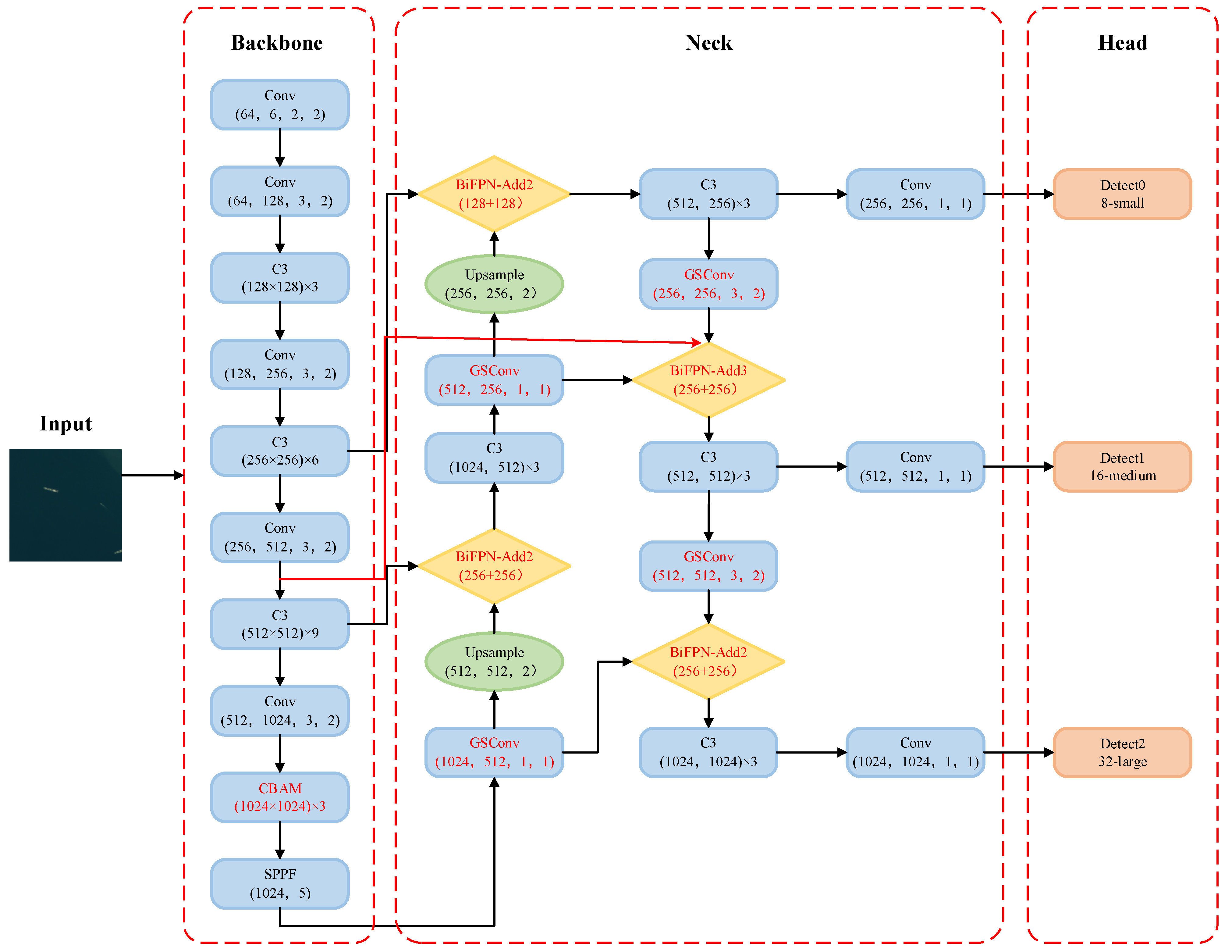
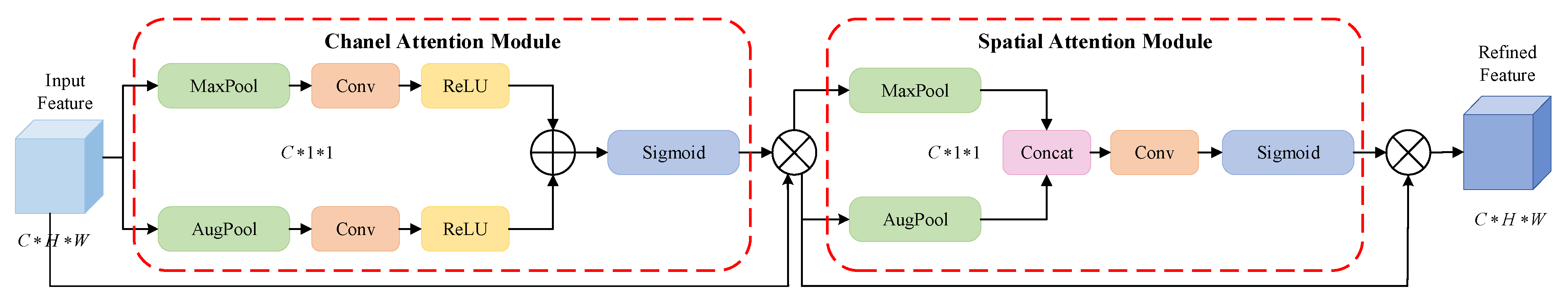
• Adding the Convolutional Block Attention Module (CBAM) [20] in the backbone network to focus on regions of interest, suppress useless information and improve the feature extraction capability;
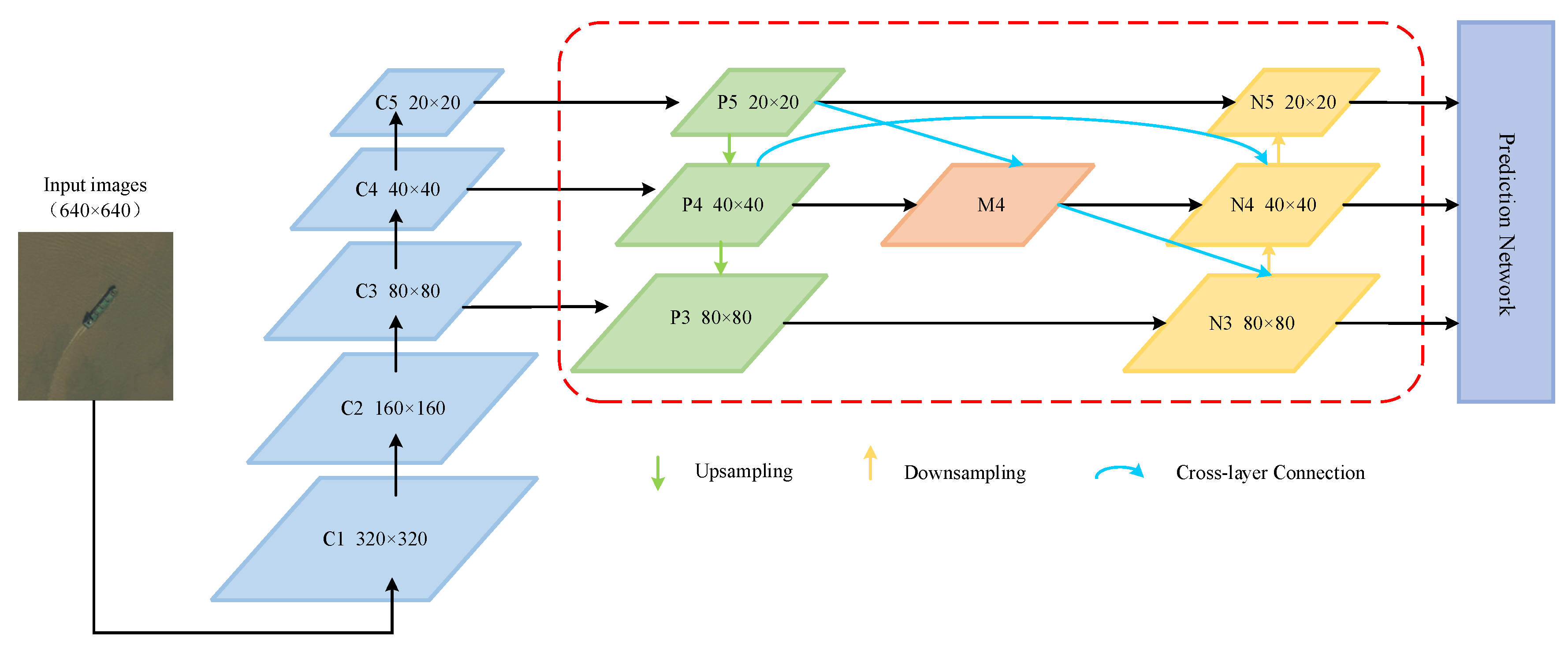
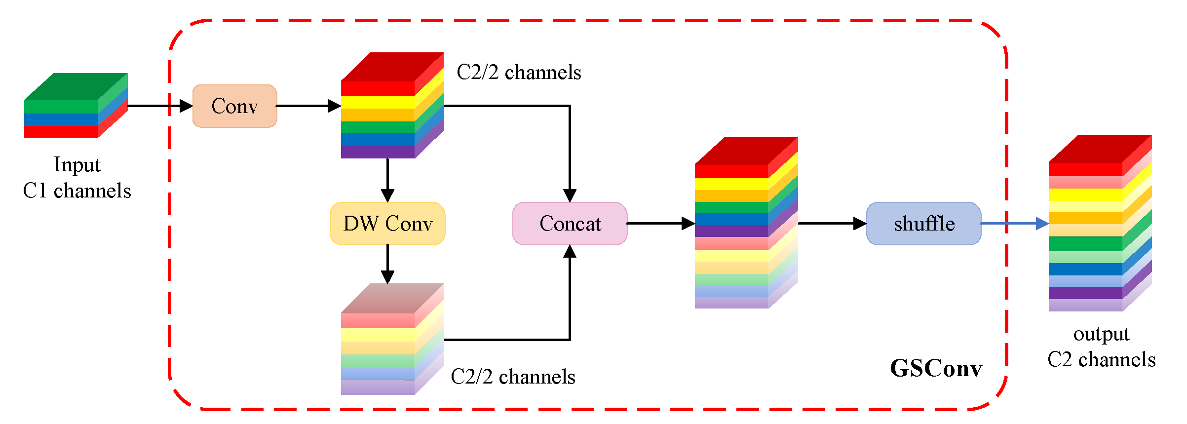
• Inspired by the Weighted Bi-directional Feature Pyramid Network (BiFPN) [21], adding an additional cross-layer connection channel in the Neck to enhance multi-scale feature fusion. Moreover, the lightweight GSConv structure [22] is introduced to replace conventional Conv, reducing the model parameters and accelerating convergence speed.
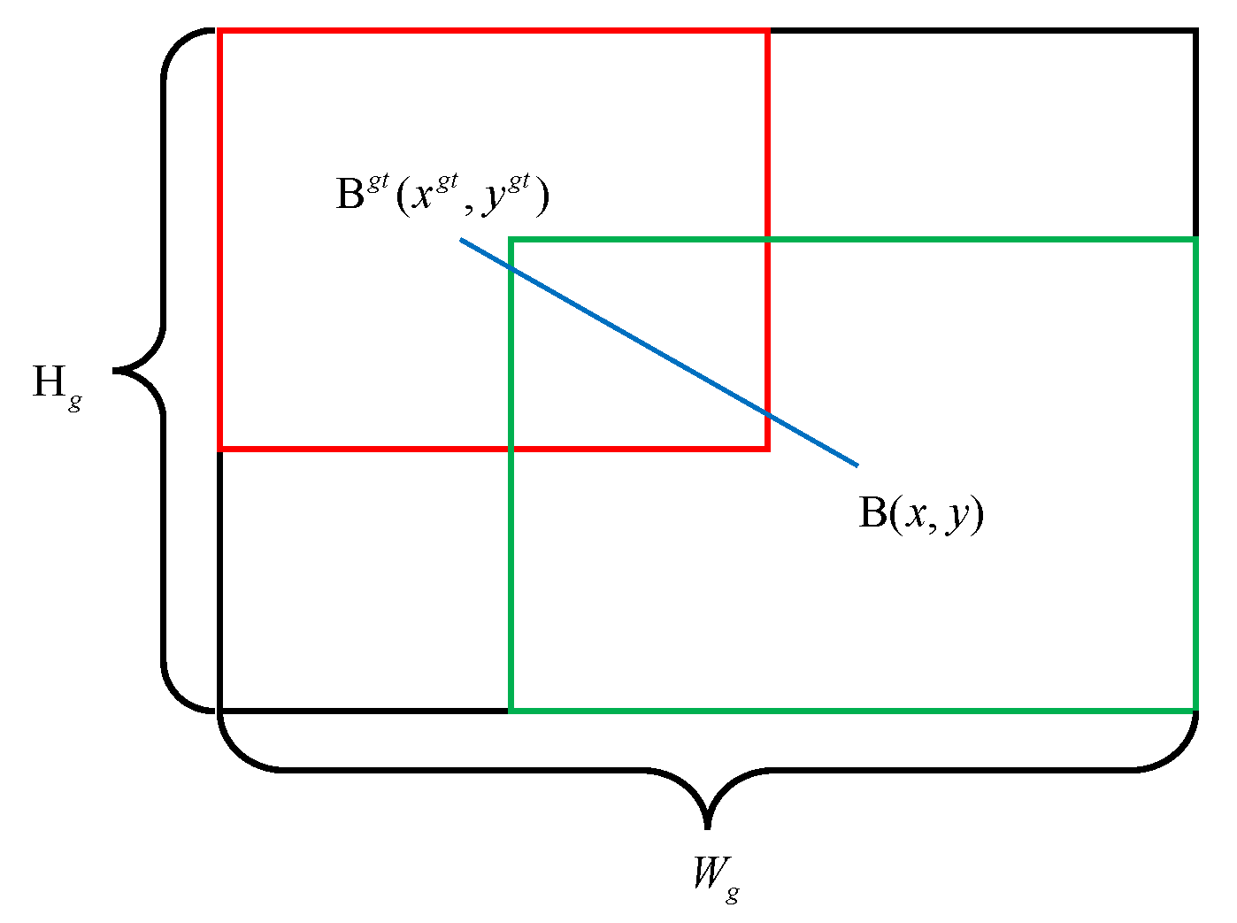
• The Wise-IoU loss function [23] is employed as the localization loss function at the Output to reduce the competitiveness of high-quality anchor boxes and mask the harmful gradients of low-quality examples.
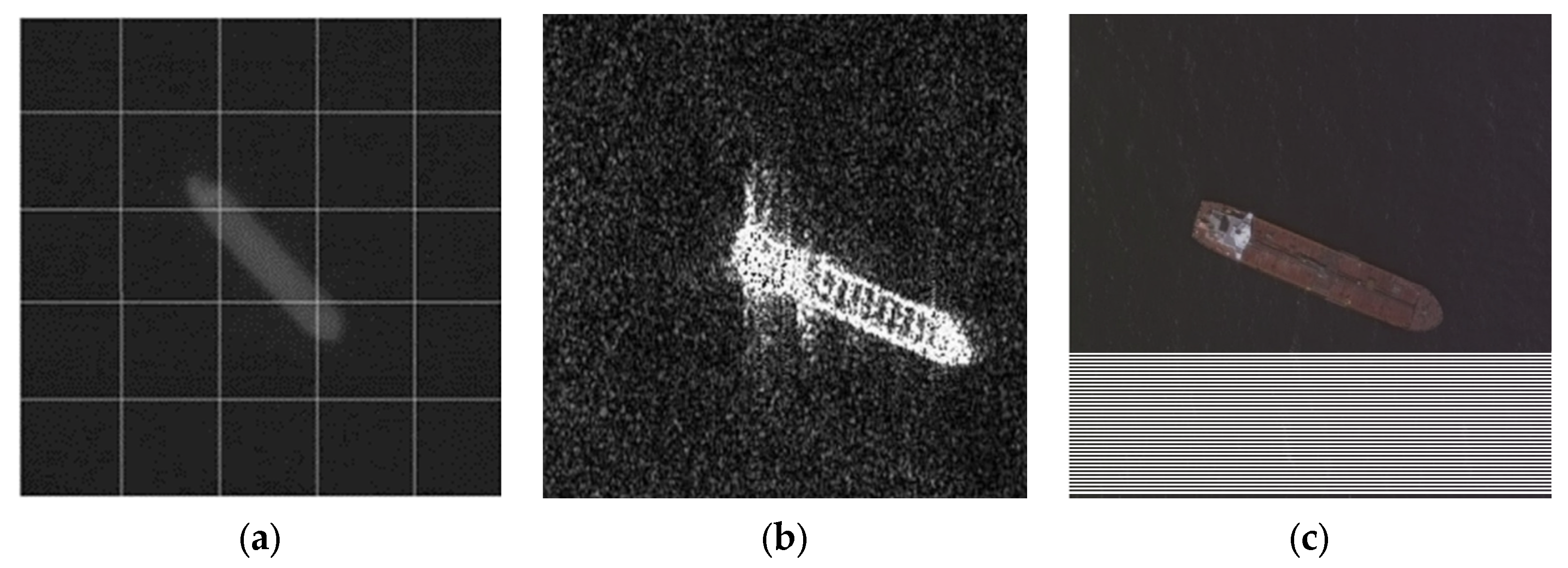
• During the preprocessing stage of experimental data, a median+bilateral filter method is used to reduce noise, such as water ripples and waves, and to highlight the ship feature information.

The above strategies can effectively improve the problem of low accuracy of fine-grained classification recognition of multi-scale and small targets in complex scenes.

3. YOLOv5 Target Detection Algorithm

As a classic model of ONE-STAGE algorithms, YOLOv5 has a relatively fast detection speed. Based on differences in network depth and width, there are four versions of YOLOv5s, YOLOv5m, YOLOv5l, and YOLOv5x, among which YOLOv5s is the smallest network and has the fastest running speed [24]. In this study, YOLOv5s is chosen as the baseline model to carry out improvement work, so as to meet the requirements of real-time ship target detection.

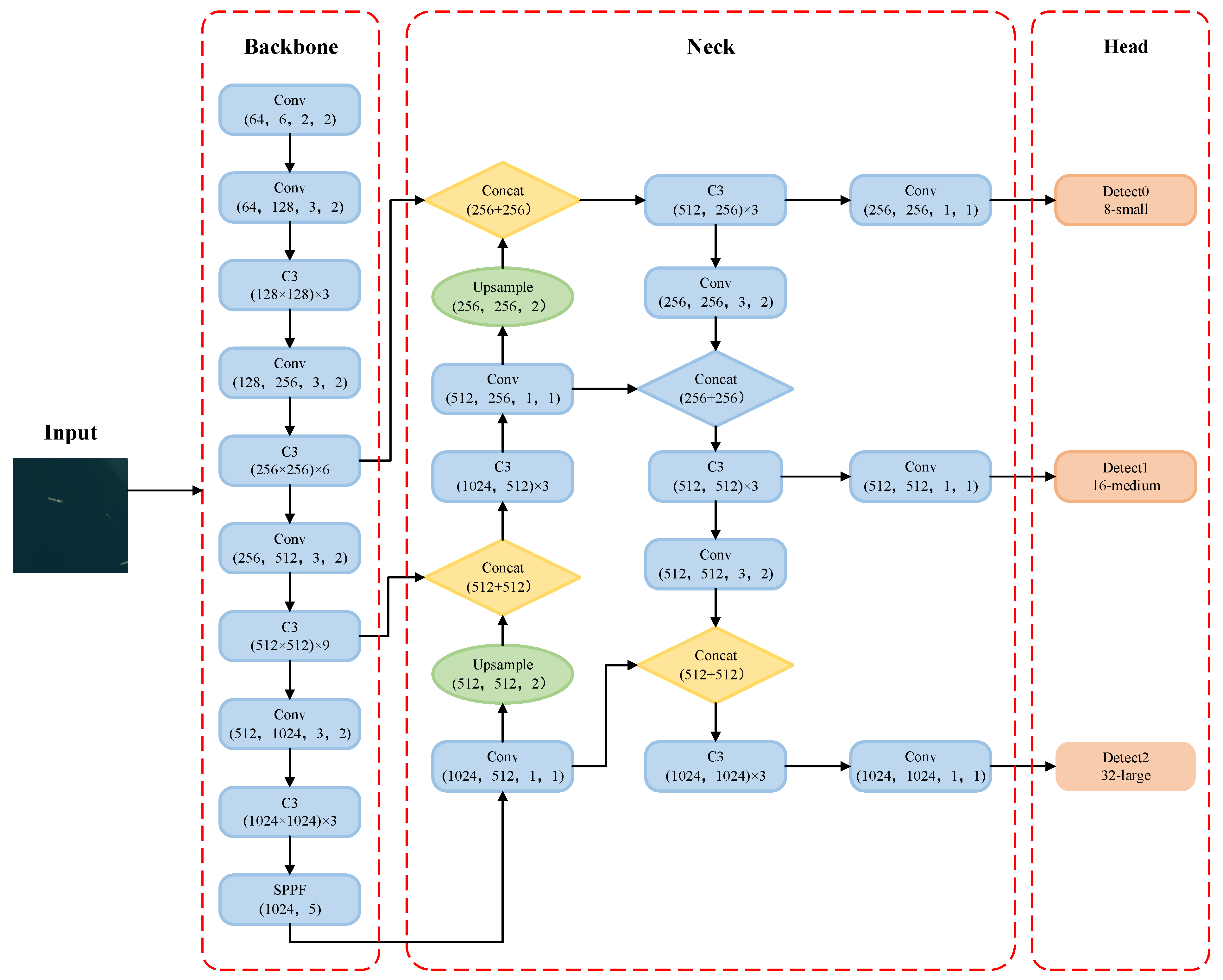
3.1. Network Structure

The YOLOv5s consists of four main parts: Input, Backbone, Neck, and Head [24]. The network structure is illustrated in Figure 2.

The Input component mainly performs preprocessing data operations, including Mosaic data enhancement, adaptive anchor frame calculation and adaptive image scaling [25] These techniques improve the training speed and network accuracy of the model.

The Backbone component adopts CSPDarknet53 as the backbone network [26], which mainly includes Conv (Conv2d+BN+SiLU) structure, C3 structure, and SSPF module. The network prevents overfitting and accelerates model convergence through Batch Normalization (BN); the C3 structure integrates gradient changes into the feature map to reduce computation while maintaining accuracy; the SPPF is an enhanced version of Spatial Pyramid Pooling (SPP), which further improve the running speed while preserving the original function.

The Neck component adopts the FPN+PAN structure, with Feature Pyramid Network (FPN) [27] passing semantic information from top to bottom and Path Aggregation Network (PAN) [28] transmitting low-level semantic and positioning information from bottom to top, thereby enhancing semantic expression and positioning capability of multiple scales.

The Head component predicts target features, generates bounding boxes, and identifies the target category.

3.2. Loss Function

The YOLOv5 loss can be divided into three main components: classification loss, objectness loss, and localization loss [29]. The overall loss is shown in Equation (1).

$$L={\lambda }_1{L}_{\mathrm{cls}}+{\lambda }_2{L}_{\mathrm{obj}}+{\lambda }_3{L}_{loc}$$

(1)

where $\lambda$ is the balance coefficient with values of 0.5, 1, and 0.05, respectively.

YOLOv5 uses Binary Cross Entropy Loss function (BCE Loss) to calculate classification loss and objectness loss. BCE loss is defined as:

$$L_{BCE}=-y\log p-\left(1-y\right)\log \left(1-p\right)==\left\{\begin{array}{c}-\log p\\ -\log \left(1-p\right)\end{array}\right.\begin{array}{c},y=1\\ ,y=0\end{array}$$

(2)

where $y$ represents the label of the input sample (positive sample is 1, negative sample is 0); $p$ represents the probability of the model predicting the input sample as a positive sample. Assuming that $p_t=\left\{\begin{array}{c}p\\ 1-p\end{array}\right.\begin{array}{c},y=1\\ ,y=0\end{array}$, the definition of BCE Loss Equation can be simplified as:

$$L_{BCE}=-\log p_t$$

(3)

The localization loss employs the C-IoU loss function, which takes into account geometric relationships such as overlap area, centroid distance and aspect ratio, and also effectively addresses the divergence problem during subsequent training. Its definition is mainly calculated from the Intersection over Union (IoU) [30], $L_{C-IoU}$ is formulated as in Equation (4).

$$L_{C-IoU}=1-IoU+\frac{{\rho }^2\left(b,b^{gt}\right)}{c^2}+\alpha v$$

(4)

Of which:

$$L_{C-IoU}=1-IoU+\frac{{\rho }^2\left(b,b^{gt}\right)}{c^2}+\alpha v$$

$$v=\frac{4}{{\pi }^2}{\left(\arctan \frac{w^{gt}}{h^{gt}}-\arctan \frac{w}{h}\right)}^2$$

where ${\rho }^2\left(b,b^{gt}\right)$ is the Euclidean distance between the center point of the prediction box and ground truth box, also known as $b$; $c$is the diagonal length of the minimum bounding box between the prediction and ground truth box; $\alpha$ is the weight coefficient; $v$ is used to measure the consistency of the aspect ratio; $gt$ is the ground truth box; $w$ and $h$ are the width and height of the prediction box, respectively.

4. Improved-YOLOv5 Target Detection Algorithm

The paper proposes an Improved-YOLOv5 algorithm for ship target detection in optical remote sensing imagery, with the overall network architecture is shown in Figure 3.

During the improvement process of the Backbone Network, the CBAM module [20] is added, which combines channel and spatial attention modules to make the feature extraction by focusing more on the target area and suppressing useless information. In the Neck structure, the BiFPN [21] is used to introduce contextual [31] and weight information, which helps in balancing features of different scales. Furthermore, an additional cross-layer connection channel is added to generate a larger receptive field and richer semantic information, this will achieve higher-level multi-scale feature fusion. Meanwhile, all Conv modules were replaced by GSConv modules [22] to reduce the parameters and computation brought about by the feature pyramid structure upgrades [5]. Finally, the Wise-IoU loss function is used to calculate the localization loss in the Output. By re-evaluating the quality of anchor boxes, a wise gradient gain allocation strategy is provided, which can effectively reduce the competitiveness of high-quality anchor boxes while also reducing harmful gradients generated by low-quality examples [23].

4.1. CBAM Attention Module

As the hierarchical depth of the network increases, the information extracted from the head of the YOLOv5s network becomes increasingly abstract which will lead to missed or false detection of small objects in the image [5]. Meanwhile, in remote sensing imagery, the majority of ship detection targets occupy a relatively small proportion of the entire image. The feature information extracted from these targets is often small and inconspicuous, so the CBAM [20] is added to the Backbone Network to obtain information of interest, suppress useless information, and enhance the ability to extract feature information for small targets. The working principle of the CBAM module is illustrated in Figure 4.

The CBAM consists of two main sub-modules, Channel Attention Module (CAM) and Spatial Attention Module (SAM) [32]. How it works: Firstly, CAM changes the feature map from $C \ast H \ast W$ to $C \ast 1 \ast 1$ through maximum pooling and average pooling, then after the Conv module and the ReLU activation function, the two activated results are summed element by element, then the output of the CAM is obtained through the Sigmoid activation function, and finally multiplied with the original map, which becomes the $C \ast H \ast W$ size again. Secondly, SAM takes the output of the CAM as input, and also passes through the MaxPool and AugPool layers to obtain two $C \ast 1 \ast 1$ feature maps, which are transformed into a 1-channel feature map through concatenating and $7 \ast 7$ Conv, and then passes through the Sigmoid activation function to obtain the output of SAM, which is finally multiplied with the original map to revert to the $C \ast H \ast W$ size. The CBAM can effectively focus on the local information region and improve the feature extraction capability.

4.2. Multi-Scale Feature Fusion

4.2.1. BiFPN Network

In the feature fusion part, the original network employs a top-down Feature Pyramid Network (FPN) [27] structure to achieve feature fusion of shallow location and deep semantic information. However, due to the unidirectional information flow, a bottom-up Path Aggregation Network (PAN) [28] pathway is added to reduce information loss. Nevertheless, this structure lacks direct connections between two nodes at the same level, which limits the degree of multi-scale feature fusion that can be achieved. In this study, BiFPN structure is introduced without adding too much computational cost [33], as shown in Figure 5. The importance of different input streams is determined by learnable weighting factors, while an additional cross-layer connection channel is added between two nodes to enable higher-level multi-scale feature fusion.

The feature map $C4$ is chosen as an example to illustrate the feature fusion process based on the incorporation of cross-scale connection and contextual information weighting operations.

Firstly, each input stream needs to be assigned a weight factor, and the weights are obtained by means of network self-learning, using the fast normalized fusion method [21] to constrain the size of each weight, which is calculated as shown:

$$O={\displaystyle {\sum }_i\frac{{\omega }_i\cdot X_i}{\epsilon +{\displaystyle {\sum }_j{\omega }_j}}}$$

(5)

where: $O$ is the output feature map; ${\omega }_i$ and ${\omega }_j$ are the learning weight coefficients of the feature map in layers $i$ and $j$, respectively; $X_i$ is the input feature map; $\epsilon \le 0.001$.

Secondly, it can be observed that the input streams of feature map $N4$ include $P4$, $M4$ and $N3$, where $M4$ is the image map of feature maps $P4$ and $P5$, and its calculation process is shown in Equation (6):

$$N_4=C\mathrm{onv}\left(\frac{{{\omega }^{\prime }}_1{P}_4^{in}+{{\omega }^{\prime }}_2{P}_4^{td}+{{\omega }^{\prime }}_3\cdot \mathrm{Resize}\left(P_3^{out}\right)}{{\omega }_1+{\omega }_2+{\omega }_3+\epsilon }\right)$$

(6)

where: $Conv$ is the convolution operation; ${\omega }_i$, ${\omega }_i^{’}$ are the different layer learning weights; $P_i^{in}$ and $P_i^{out}$ are the input and output of layer $i$, respectively; $P_i^{td}$is the output of the middle node of the feature map in layer $i$; $Res\mathrm{ize}$ refers to maintaining the consistency of the input feature map size by using upsampling or downsampling operations; and $\epsilon$is usually set to $0.0001$.

4.2.2. GSConv Structure

As the network deepens, the feature map gradually transmits spatial information to the channels during the backbone network feature extraction process. However, spatial compression and channel expansion operations lead to partial loss of semantic information. To address this issue, this paper uses lightweight GSConv structure [22] to replace the conventional Conv. This structure can alleviate the resistance of the input stream and reduce the complexity of the model, while greatly preserving each inter-channel hidden connections and spatial information without any compression processing. The structure is demonstrated in Figure 6.

4.3. Loss Function

A well-designed localization loss function plays a crucial role in the object detection loss function, as it can greatly enhance the performance of object detection models. In the real scene, there are some low-quality images, and the dataset in this paper is no exception. Geometric factors (such as distance and aspect ratio) will exacerbate the penalty for low-quality examples, thus reducing the generalization performance of the model. Based on dynamic non-monotonic focusing mechanism, Wise-IoU loss function is constructed to calculate the localization loss, which has three versions, namely W-IOU_v1, W-IOU_v2, and W-IOU_v3 [23]. In this paper, utilizing the W-IOU_v3 outlier degree to re-evaluate the quality of anchor boxes based on W-IOU_v1, and assigning different gradient gains to samples of different qualities. Figure 7 illustrates a schematic diagram of the calculation of each parameter in the Wise-IoU loss.

The W-IOU_v1 loss function is defined as:

$$L_{W-Io{U}_{v1}}=R_{W-IoU}{L}_{IoU}$$

(7)

Of which:

$$R_{W-IoU}=\exp \left(\frac{{\left(x-x_{gt}\right)}^2+{\left(y-y_{gt}\right)}^2}{{\left(W_g^2+H_g^2\right)}^{\ast }}\right)$$

$$L_{IoU}=\frac{B\cap B^{gt}}{B\cup B^{gt}}$$

where: $(x,y)$ and $(x_{gt},y_{gt})$ are the coordinate values of the center points of the prediction and ground truth box; $W_g,H_g$ are the width and height of the minimum bounding box between the prediction and ground truth box; $B,B_{gt}$ are the areas of the prediction and ground truth box.

W-IOU_v3 introduces the outlier degree to describe the quality of the anchor box on based on W-IOU_v1, it is defined as:

$$\beta =\frac{L_{IoU}^{\ast }}{\overline{L_{IoU}}}\in \left[0,+\infty \right)$$

(8)

A smaller outlier degree indicates a higher quality anchor box and is given a smaller gradient gain in order to concentrate the localization loss on regular anchor boxes; in addition, a larger outlier degree assigned a smaller gradient gain can effectively prevent harmful gradients from low quality examples.

Thus, the non-monotonic focusing mechanism factor $r$ constructed using the outlier degree is applied to W-IOU_v1, the definition of W-IOU_v3 is as follows:

$$L_{W-Io{U}_{v3}}=r{L}_{W-Io{U}_{v1}}$$

(9)

Of which:

$$r=\frac{\beta }{\delta a^{\beta -\delta }}$$

5. Experimental Results and Analysis

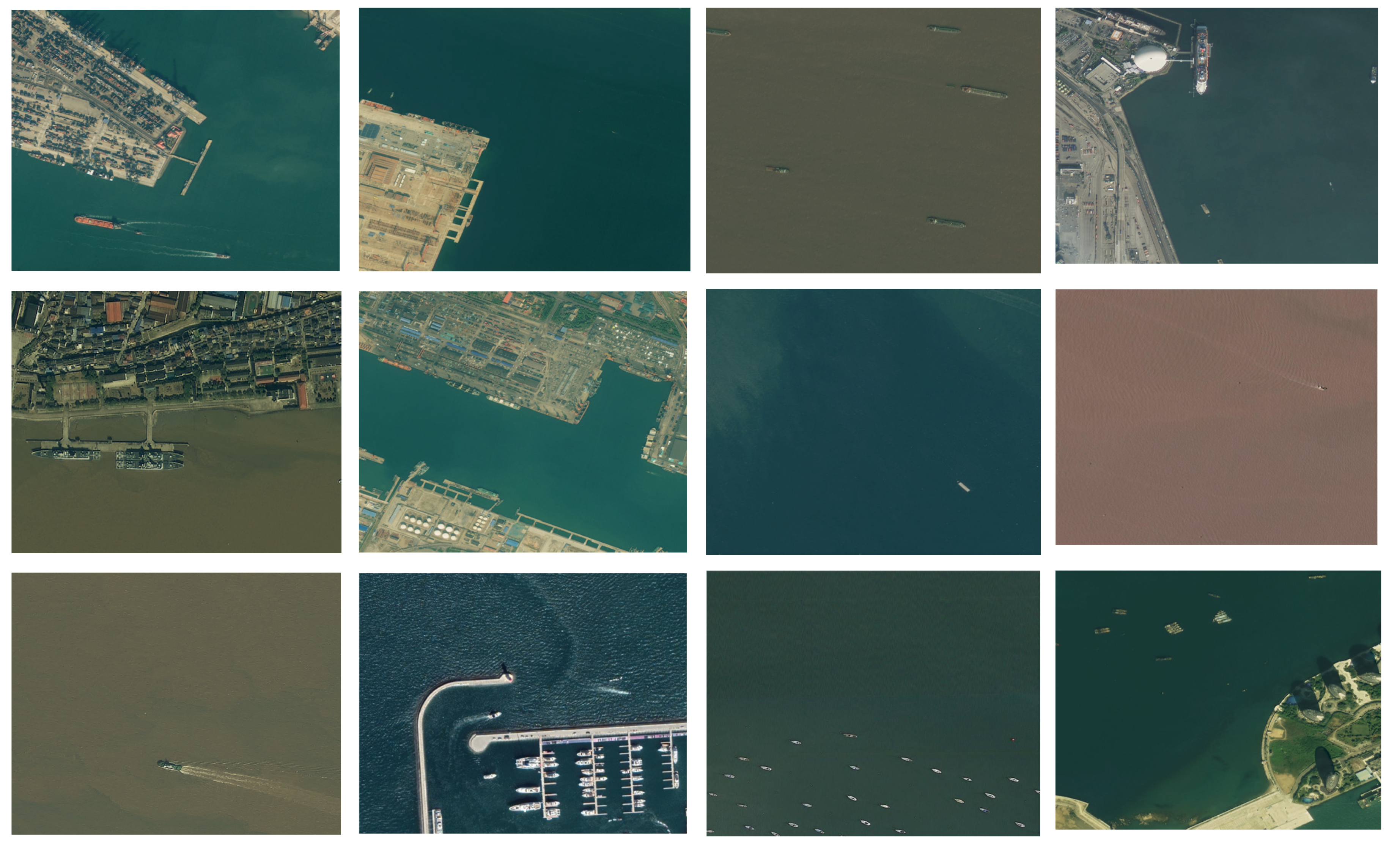
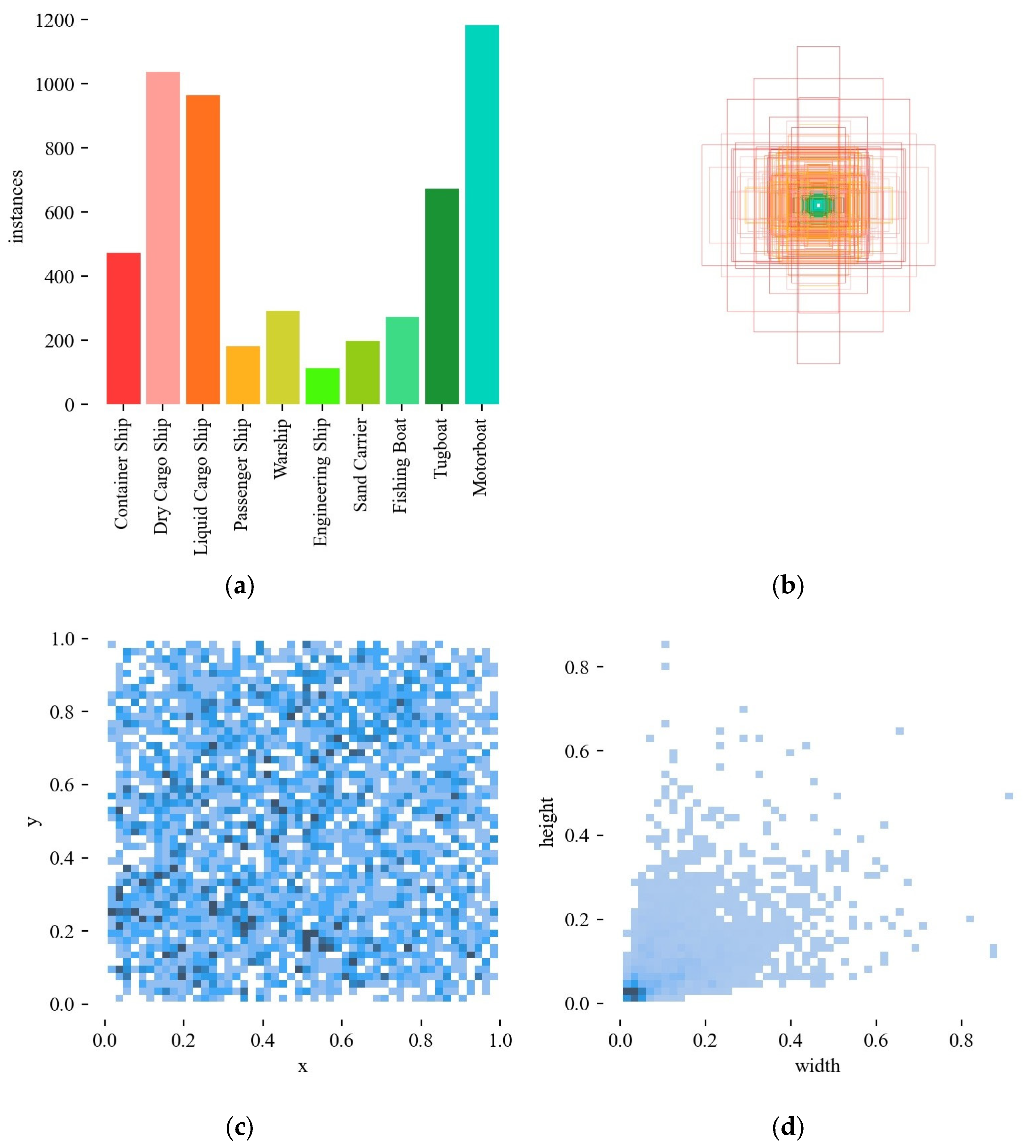
5.1. Experimental Dataset

The dataset for this experiment was chosen from the Fine-grained Object Recognition in High-resolution Remote Sensing Imagery (FAIRIM) [34] created by the Aero-space Information Research Institute of the Chinese Academy of Sciences. The dataset covers various scenes such as nearshore ports and offshore areas. This study has selected 2235 images and manually annotated them into 10 common types of ships (Container Ship (CS), Dry Cargo Ship (DCS), Liquid Cargo Ship (LCS), Passenger Ship (PS), Warship (WS), Engineering Ship (ES), Sand Carrier (SC), Fishing Boat (FB), Tugboat (TB), and Motorboat (MB)). In addition, the dataset is divided into a training set (80%) and a validation set (20%). Some of example images in the FAIRIM dataset are shown in Figure 8.

The visualization results of the dataset are presented in Figure 9. Figure 9a shows the types of vessels and the number of each category labelled in this dataset; Figure 9b can see intuitively the distribution of anchor boxes for the data labels; and Figure 9c reveals the relative position of the detection targets compared to the whole image coordinate system. Figure 9d is the normalized target size map, which means the size of the detection target in relation to the whole image [35], it can be seen from the figure that the target size distribution is relatively concentrated and mostly small.

5.2. Experimental Platform and Parameters Setting

The experimental platform configuration used in this study is shown in

Table 1. Experimental environment configuration.

Parameter	Configuration
Operating Environment	Windows 11
GPU	GeForce RTX 3050
Programming Language	Python 3.7
Programming Platform	Pycharm
Deep Learning Framework	Pytorch 1.13.0
CUDA	11.0
CuDNN	8.0

.

The network model training was conducted under the experimental environment described above, and the training parameters are shown in

Table 2. Experimental parameters setting.

Parameter	Number
Img-size	640 × 640
Batch-size	8
Epochs	300
Learning rate	0.01
Momentum	0.937
Weight-decay	0.0005

.

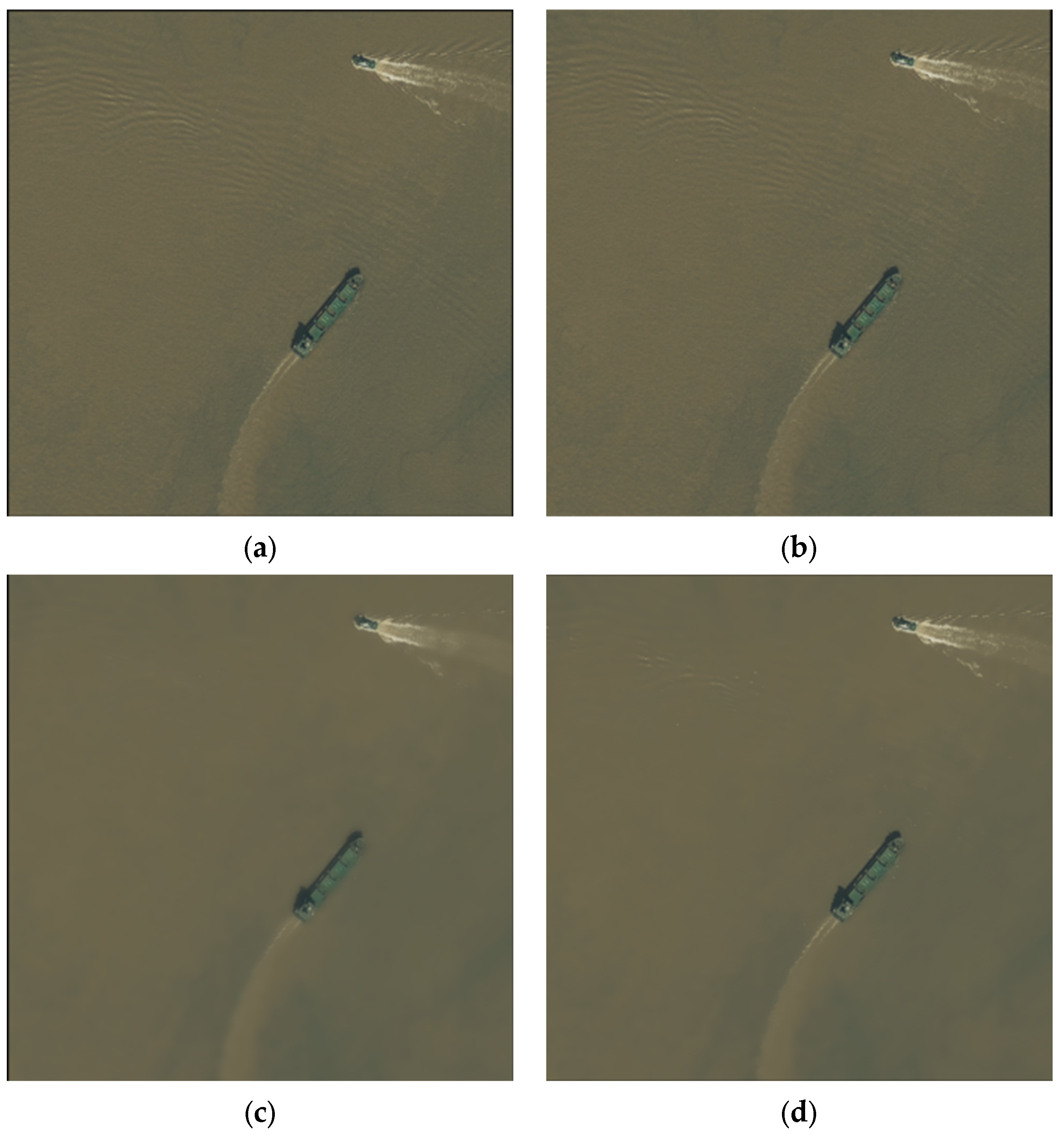
5.3. Image Preprocessing

To eliminate the interference of water ripples, waves, wakes, and salt and pepper noise around the ship and highlight the information of ship features, this paper combines median and bilateral filter method for noise reduction of the images.

Median Filter (MF) involves replacing the pixel value of a point in an image with the median value of the values of all points in its neighborhood. This makes the surrounding pixel values closer to the true values, thereby eliminating isolated noise points [36]. An example of this is shown in Figure 10.

Bilateral Filter (BF) is a non-linear filter that takes into account the influence weight of the Euclidean distance and the grey scale interpolation when calculating the new value of a certain pixel point [37]. It can effectively remove noise and preserve the edge features of ships better. The definition is as follows:

$$BF{\left[I\right]}_p=\frac{1}{W_p}{\displaystyle \sum _{q\in S}{G}_{{\sigma }_s}}\left(‖p-q‖\right)G_{{\sigma }_r}\left(\left|I\left(p\right)-I\left(q\right)\right|\right)I\left(q\right)$$

(10)

Of which:

$$W_p={\displaystyle \sum _{q\in S}{G}_{{\sigma }_s}}\left(‖p-q‖\right)G_{{\sigma }_r}\left(\left|I\left(p\right)-I\left(q\right)\right|\right)$$

where: $BF{\left[I\right]}_p$ is the image after bilateral processing; $W_p$is the normalization factor; $S$ is the neighborhood of a pixel point; $G_{{\sigma }_S}\left(‖p-q‖\right)$ is the spatial weight; ${\sigma }_s$is the standard deviation of the spatial domain; $p,q$ are any two pixel points in the image; $G_{{\sigma }_r}\left(\left|I\left(p\right)-I\left(q\right)\right|\right)$ is the pixel range weight; ${\sigma }_r$ is the standard deviation of the range; $I\left(p\right)$ is the input image; and $I\left(q\right)$ is the output image.

Through comparison between the median filter, bilateral filter, and their combination, it is observed that the combination of median and bilateral filter has a better noise reduction effect than using them individually. Therefore, this paper adopts the median + bilateral filter method for image noise reduction in the dataset, and its noise reduction effect is shown in Figure 11.

5.4. Evaluation Metrics

In this study, the algorithm’s performance is evaluated using Average Precision (AP), mean Average Precision (mAP), and Frames Per Second (FPS) as the evaluation metrics.

The AP is a measure of the quality of detection results for a certain category, usually related to Recall (R) and Precision (P); The mAP is a measure of detection results for multiple categories, and its calculation is related to the AP; The Equation for calculating AP and mAP are as follows.

Recall (R) is calculated by the Equation:

$$R=\frac{N_{TP}}{N_{TP}+N_{FN}}$$

where: $N_{TP}$ is the number of positive samples that are correctly classified; $N_{FN}$ is the number of samples that are positive but are misclassified as negative.

Precision (P) is calculated by the Equation:

$$P=\frac{N_{TP}}{N_{TP}+N_{FP}}$$

where: $N_{FP}$ is the number of samples that are negative but are misclassified as positive.

The AP is the area enclosed by the P-R curve, with Precision and Recall as the vertical and horizontal coordinates, which is calculated as:

$$AP={\displaystyle {\int }_0^{1}P(r)dr}$$

(11)

The AP of all samples were then averaged to obtain the mAP, which is calculated as:

$$mAP=\frac{{\displaystyle \sum AP}}{N_{all\_classes}}$$

(12)

where: $N_{all\_classes}$ is the total number of samples. mAP_0.5 and mAP_0.5:0.95 are two representations of the mAP. The mAP_0.5 sets the IoU threshold to 0.5 and then averages the AP for all classes; The mAP_0.5:0.95 sets different thresholds ranging from 0.5 to 0.95 with a step size of 0.5, and then averages the AP for all classes.

The FPS stands for frames per second, is the main indicator for real-time performance evaluation of a model, which is calculated as:

$$FPS=\frac{1000}{t_p+t_i+t_{NMS}}$$

(13)

where: $t_p$ is the image preprocessing time; $t_i$ is the model inference time; $t_{NMS}$ is the Non-Maximum Suppression time.

5.5. Ablation Experiment

This paper performed seven ablation experiments in order to assess the effectiveness of different improvements on the model performance. The specific improvement strategies include the CBAM module, BiFPN network, GSConv and Wise-IoU loss function. The target’s height and width in pixel values and categorize its dataset into Large-size (256 pixels × 256 pixels), Medium-size (128 pixels × 128 pixels), and Small-size (64 pixels × 64 pixels) [38]. The results of the ablation experiment are shown in

Table 3. Detailed comparison of the results of the ablation experiment. “×” means not applied, and ”√” verse vita.

Improvement Strategy			AP (%)										mAP_0.5 (%)	FPS (f/s)
			Large-Size				Medium-Size			Small-Size
CBAM	BiFPN+GSConv	W-IoU	CS	DCS	LCS	PS	WS	ES	SC	FB	TB	MB
×	×	×	88.4	93.4	88.7	73	97.6	47.4	56.5	76.7	59	68	74.9	69
√	×	×	91.3	93.2	89.5	78.7	97	52.7	58	85.2	57.4	67.7	77.1	67
×	√	×	88.1	94.5	87.6	79.6	98.3	53.7	65.4	81.9	53.3	67.5	77	69
×	×	√	89.8	94	87.8	80.5	96.6	55.7	60.4	83.7	56.8	67.5	77.3	71
√	√	×	91.2	93.9	90.4	81.9	95.4	55.2	55.9	84.9	53.5	66.5	76.9	76
√	×	√	89.3	92.9	87.6	77.8	97.4	56.2	58.1	79	47.5	63.8	75	76
×	√	√	89.2	94.7	88.9	78	97.7	61.7	47.4	81.7	54	64.7	75.8	76
√	√	√	89.9	93.9	87.9	82.9	96	59.3	61.3	82.7	58.8	68.6	78.1	75

, with the best results in bold.

Firstly, this paper adds CBAM module in the backbone network to suppress irrelevant information and focus more on the target information. Secondly, the neck is replaced with the BiFPN network to enable feature fusion at different levels, while the regular Conv is replaced with GSConv structures to reduce model parameters and shorten training time. Finally, using the Wise-IoU loss function to calculate the localization loss, it can effectively reduce the competitiveness of high-quality anchor boxes and harmful gradients generated by low-quality examples.

As can be seen from Table 3, in the ablation experiments, the improvement strategies proposed in this paper have achieved certain improvements in the detection performance indicators. Compared to the original YOLOv5, the mAP_0.5 of the individual improvement strategy increased by 2.2%, 2.1%, and 2.4%, respectively, the combination of the two improvement strategies increased by 2%, 0.1%, and 0.9%, respectively, and finally the combination of all improvement strategy increased by 3.2%. Ultimately, the improvement scheme was determined to include the CBAM, BiFPN network, lightweight GSConv structure and the W-IoU loss function. The experimental results before and after its improvement with the original model YOLOv5 are shown in Figure 12.

As shown in Figure 12, the Improved-YOLOv5 performs much better in AP for small and medium ships, and the overall loss is less than the original YOLOv5. In terms of mAP, mAP_0.5 and mAP_0.5:0.95 first surpassed the original YOLOv5 at about 105 and 120 epochs, respectively, and have maintained the lead ever since. In sum, after 300 epochs of training, the Improved-YOLOv5 algorithm has outperformed the original YOLOv5 in all evaluation metrics.

A confusion matrix was utilized to evaluate the accuracy of the model’s results. Each column of the confusion matrix represents the predicted proportions of each category, while each row represents the true proportions of the respective category in the data [39]. The confusion matrix for the two algorithms before and after the improvement is shown in Figure 13, as can be seen, most of the targets were correctly predicted. The improved-model has slightly better detection performance than the original model on small and medium ship targets.

The comparison of the detection performance before and after the algorithm improvement is illustrated in Figure 14.

Upon comparing the images, it can be found that the improved model can effectively improve the detection effect, avoid the situation of missed and false detection. Additionally, it enhances the ability to detect small and medium ship targets. The following images are displayed enlarged based on the original image.

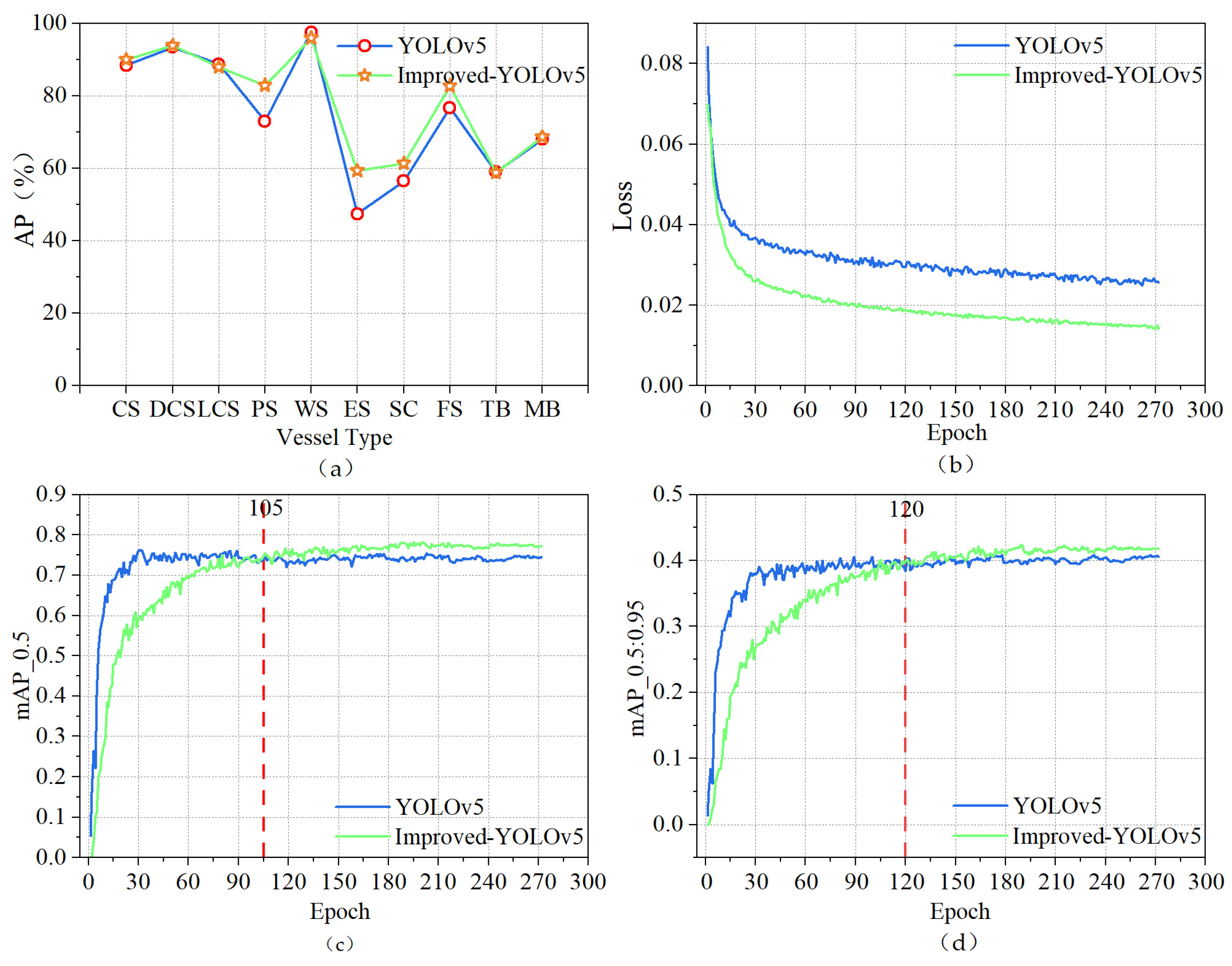
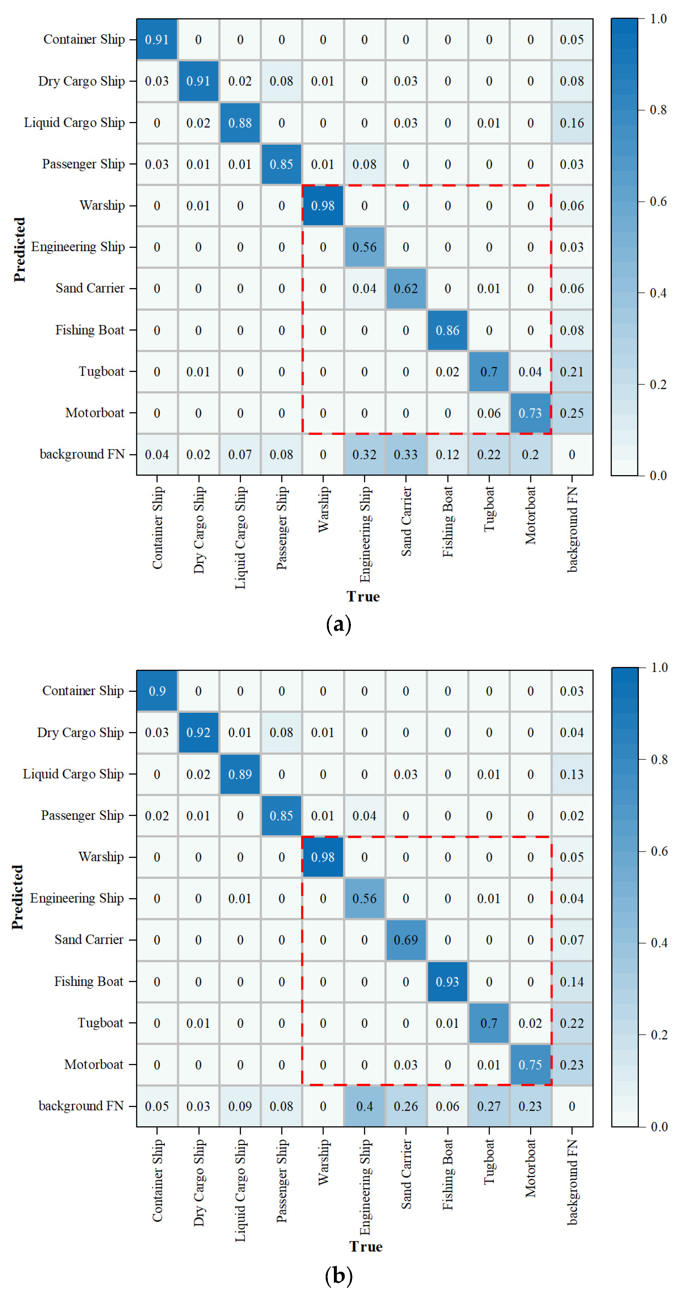
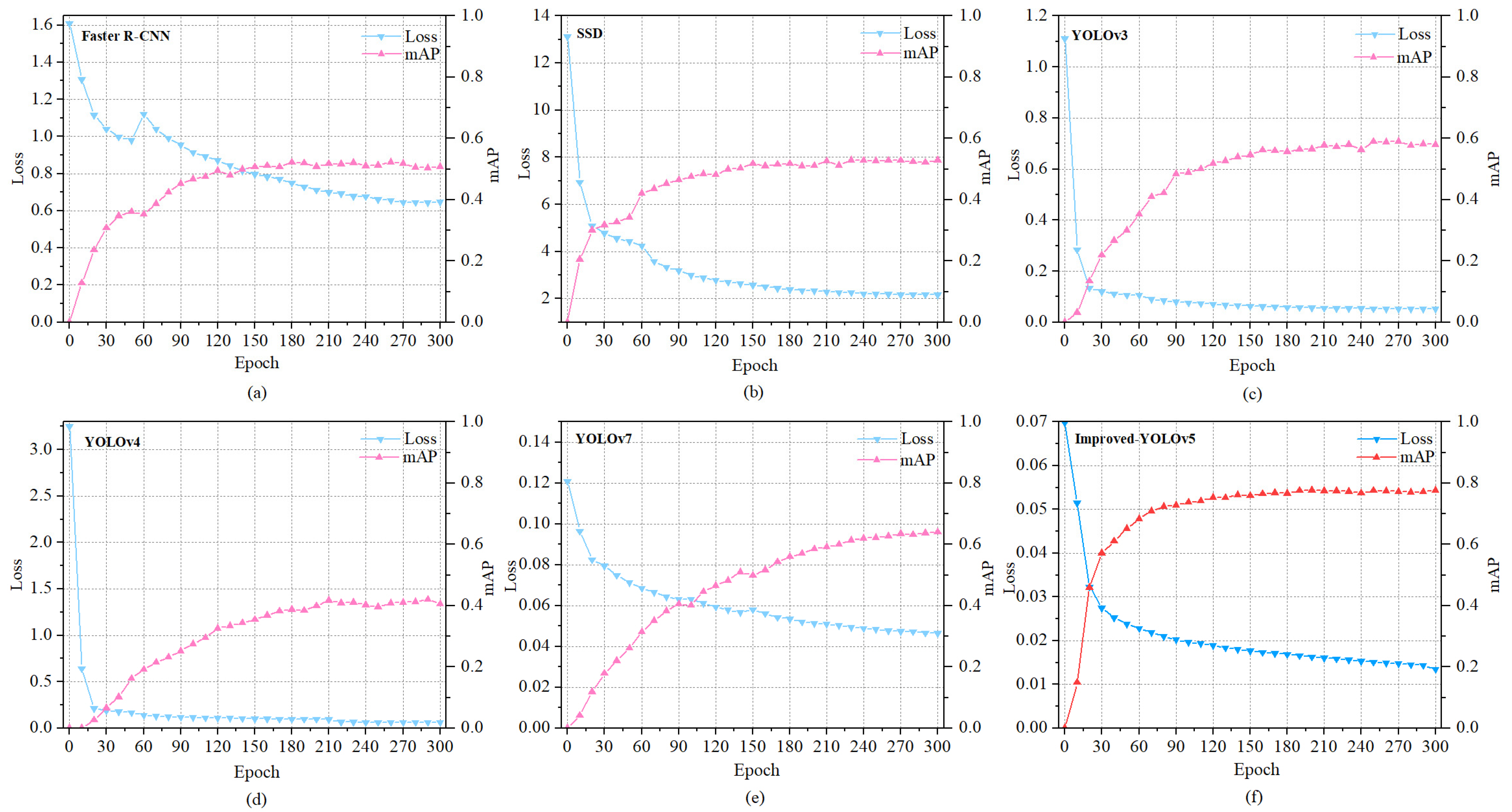
5.6. Performance Comparison of Various Target Detection Algorithms

In order to further validate the effectiveness of the improved algorithm, this study compared it with several advanced target detection algorithms, including Faster R-CNN, SSD, YOLOv3, YOLOv4, YOLOv5, YOLOv7, and YOLOv8 (see

Table 4. Comparison of detection results between different algorithms.

Modeling Algorithm	AP (%)										mAP (%)	FPS (f/s)
	Large-Size				Medium-Size			Small-Size
	CS	DCS	LCS	PS	WS	ES	SC	FB	TB	MB
Faster R-CNN	95.7	76.3	81.6	72	94.6	48.2	16.4	25.9	10.1	16.9	53.8	7
SSD	92.3	73.9	82.3	77.3	88.3	37.1	16.3	73.8	19.5	19.3	57.9	45
YOLOv3	93.9	72.7	84.6	85	92	26.2	10.2	55.7	38.7	50.8	60.9	33
YOLOv4	78.2	69.5	79.1	72.3	77.4	0	0	0	12.9	42.5	43.2	41
YOLOv5	88.4	93.4	88.7	73	97.6	47.4	56.5	76.7	59	68	74.9	69
YOLOv7	84.3	89.9	73.9	76.8	96.4	34	26.5	79.1	27	54..6	64.3	35
YOLOv8	86.6	93.8	88.1	80.7	96.9	54.3	61.6	79.9	60.2	68.7	77.3	46
Improved-YOLOv5	89.9	93.9	87.9	82.9	96	59.3	61.3	82.7	58.8	68.6	78.1	75

, with the best results in bold).

From the experimental results, it can be observed that the Improved-YOLOv5 proposed in this study achieves the best detection performance on the FAIRIM dataset, with the mAP of 78.1%. Improved-YOLOv5 has increased 24.3%, 20.2%, 17.2%, 34.9%, 3.2%, 13.8%, and 0.8% in the mAP compared to Faster R-CNN, SSD, YOLOv3, YOLOv4, YOLOv5, YOLOv7, and YOLOv8, respectively. In addition, YOLOv8 and Improved-YOLOv5 have an excellent performance in detecting small and medium ships. However, YOLOv8 is not as good as Improved-YOLOv5 in terms of detection effect and recognition accuracy. Furthermore, the FPS of Improved-YOLOv5 is significantly improved compared to other model algorithms, which better meet the requirements for real-time target detection. The experimental comparison results of training loss and the mAP of Improved-YOLOv5 and various target detection algorithms are shown in Figure 15.

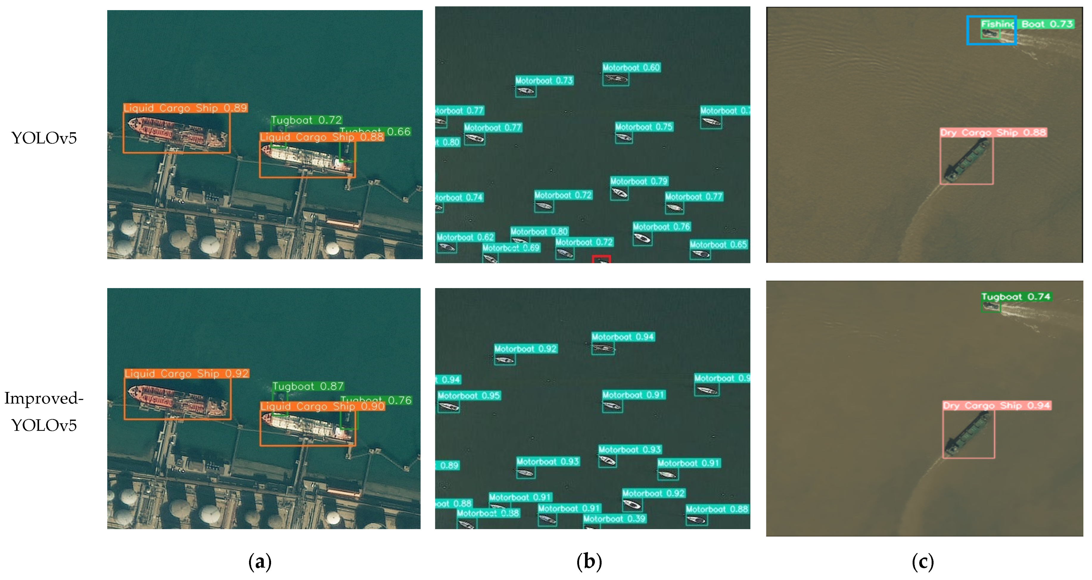
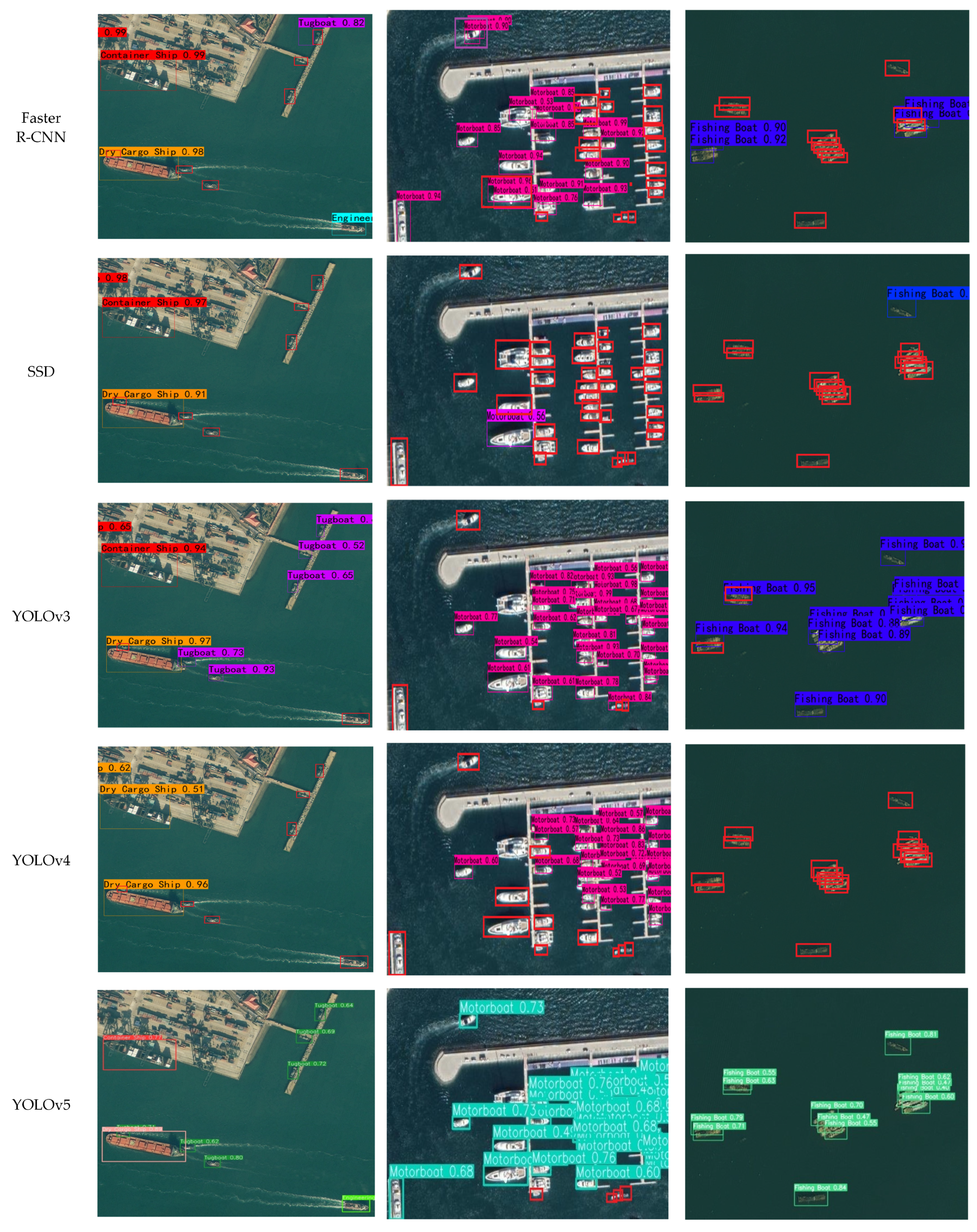
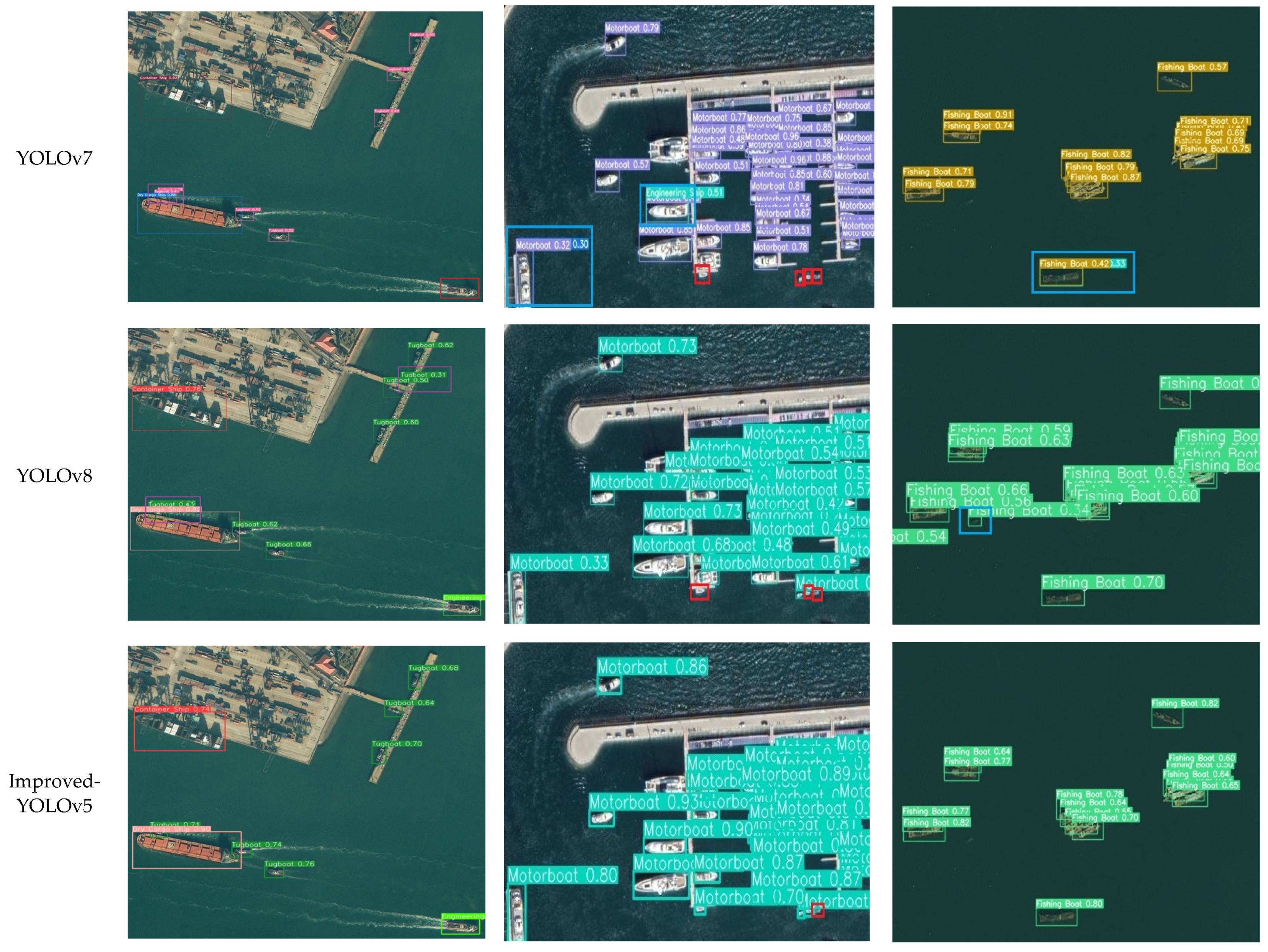
5.7. Comparison of Detection Results

Due to the distance and angle of remote sensing satellite imaging, the size of ship targets in the entire image is relatively small. This limitation results in feature information is insufficient in the network extraction process and leads to unsatisfactory detection performance of the current various target detection algorithms. In order to effectively verify the detection performance of our algorithm and several commonly used algorithms in complex scenes, we compared the proposed method with seven typical methods (Faster R-CNN, SSD, YOLOv3, YOLOv4, YOLOv5, YOLOv7, and YOLOv8). Figure 16 visually shows the ship detection results in different maritime scenes. Complex scenes include situations such as multi-scale, a large number of small and tight arranged targets. Compared to the others, our proposed improved method can efficiently and accurately identify ship types in different scenes captured by remote sensing satellites, especially in the detection ability of small and medium ship targets. The following images are displayed enlarged based on the original image.

The comparison in Figure 16 shows that Improved-YOLOv5 outperforms other algorithms in terms of both missed and false detections, and at the same time has a high detection accuracy. Meanwhile, it also can meet the requirements of accurate and real-time detection of ships on the sea surface from remote sensing images.

6. Conclusions

Due to the special characteristics of optical remote sensing images, the detection effect of small-sized and closely arranged targets is unsatisfactory, there are non-negligible cases of missed and false detection [4]. We have added some cutting-edge technologies based on YOLOv5. Firstly, CBAM is added to the backbone network to adaptively optimize the features of the targets in both channel and spatial dimensions, so that network focuses more on the feature regions. Secondly, a cross-layer connection channel is used in Neck to enable higher-level multi-scale feature fusion, while the lightweight GSConv module is replaced to reduce the number of parameters and computation of the model. Finally, the Wise-IoU loss function is used to assign a reasonable gradient gain in the face of image quality difference. The experimental results show that the improved-YOLOv5 has a significant improvement in detection performance compared to the original model and other algorithms, and also meets the requirements of real-time detection. Under the premise of ensuring high precision, the improved model effectively reduces the complexity of the model, significantly improves the speed of forward inference, and reduces the number of parameters in the whole model. However, the improved model still has some shortcomings. When detecting multi-scale targets, it is easy to have missed detection of some small targets, and there is still some room for improvement. At the same time, the improved model is only practiced on the ship dataset, which cannot effectively verify the universality and advancement of the improved model.

In the future, the next focus will be to find suitable datasets and compare them with object detection algorithms related to remote sensing images to verify the universality and advancement of the improved model. Eventually, the improved model is ported to an embedded platform for lightweight deployment.

References

1. Wang, B.; Dong, L.L.; Zhao, M.; Wu, H.D.; Ji, Y.Y.; Xu, W.H. An infrared maritime target detection algorithm applicable to heavy sea fog. Infrared Phys. Technol. 2015, 71, 56–62. [Google Scholar] [CrossRef]
2. Zhao, E.Z.; Dong, L.L.; Dai, H. Infrared Maritime Small Target Detection Based on Multidirectional Uniformity and Sparse-Weight Similarity. Remote Sens. 2022, 14, 5492. [Google Scholar] [CrossRef]
3. Yang, P.; Dong, L.; Xu, H.; Dai, H.; Xu, W. Robust Infrared Maritime Target Detection via Anti-Jitter Spatial–Temporal Trajectory Consistency. IEEE Geosci. Remote Sens. Lett. 2022, 19, 1–5. [Google Scholar] [CrossRef]
4. Lang, H.T.; Wang, R.F.; Zheng, S.Y.; Wu, S.W.; Li, J.L. Ship Classification in SAR Imagery by Shallow CNN Pre-Trained on Task-Specific Dataset with Feature Refinement. Remote Sens. 2022, 14, 5986. [Google Scholar] [CrossRef]
5. Liu, P.F.; Wang, Q.; Zhang, H.; Mi, J.; Liu, Y.C. A Lightweight Object Detection Algorithm for Remote Sensing Images Based on Attention Mechanism and YOLOv5s. Remote Sens. 2023, 15, 2429. [Google Scholar] [CrossRef]
6. Nie, G.T.; Huang, H. A Survey of Object Detection in Optical Remote Sensing Images. Acta Anat. Sin. 2021, 47, 1749–1768. [Google Scholar]
7. Li, K.; Fan, Y. Research on Ship Image Recognition Based on Improved Convolution Neural Network. Ship Sci. Tech. 2021, 43, 187–189. [Google Scholar]
8. Girshick, R.; Donahue, J.; Darrell, T.; Malik, J. Rich Feature Hierarchies for Accurate Object Detection and Semantic Segmentation. In Proceedings of the 2014 IEEE Conference on Computer Vision and Pattern Recognition (ICCV), Columbus, OH, USA, 23–28 June 2014; pp. 580–587. [Google Scholar]
9. Girshick, R. Fast R-CNN. In Proceedings of the 2015 IEEE international Conference on Computer Vision (ICCV), Santiago, Chile, 7–13 December 2015; pp. 1440–1448. [Google Scholar]
10. Ren, S.Q.; He, K.M.; Girshick, R.; Sun, J. Faster R-CNN: Towards Real-Time Object Detection with Region Proposal Networks. IEEE Trans. Pattern Anal. Mach. Intell. 2017, 39, 1137–1149. [Google Scholar] [CrossRef]
11. Liu, W.; Anguelov, D.; Erhan, D.; Szegedy, C.; Reed, S.; Fu, C.Y.; Berg, A. SSD: Single Shot MultiBox Detector. In Proceedings of the 14th European Conference on Computer Vision, Amsterdam, The Netherlands, 17 September 2016; pp. 21–37. [Google Scholar]
12. Redmon, J.; Kumar, S.; Divvala, K.; Girshick, R.; Farhadi, A. You Only Look Once: Unified, Real-Time Object Detection. In Proceedings of the 2016 IEEE Conference on Computer Vision and Pattern Recognition (CVPR), Las Vegas, NV, USA, 27–30 June 2016; pp. 779–788. [Google Scholar]
13. Zhang, P.P.; Xie, G.K.; Zhang, J.S. Gaussian Function Fusing Fully Convolutional Network and Region Proposal-Based Network for Ship Target Detection in SAR Images. Int. J. Antenn. Propag. 2022, 2022, 3063965. [Google Scholar] [CrossRef]
14. Wen, G.Q.; Cao, P.; Wang, H.N.; Chen, H.L.; Liu, X.L.; Xu, J.H.; Zaiane, O. MS-SSD: Multi-scale single shot detector for ship detection in remote sensing image. Appl. Intell. 2023, 53, 1586–1604. [Google Scholar] [CrossRef]
15. Chen, L.Q.; Shi, W.X.; Deng, D.X. Improved YOLOv3 Based on Attention Mechanism for Fast and Accurate Ship Detection in Optical Remote Sensing Images. Remote Sens. 2021, 13, 660. [Google Scholar] [CrossRef]
16. Huang, Z.X.; Jiang, X.N.; Wu, F.L.; Fu, Y.; Zhang, Y.; Fu, T.J.; Pei, J.Y. An Improved Method for Ship Target Detection Based on YOLOv4. Appl. Sci. 2023, 13, 1302. [Google Scholar] [CrossRef]
17. Zhou, J.C.; Jiang, P.; Zou, A.; Chen, X.L.; Hu, W.W. Ship Target Detection Algorithm Based on Improved YOLOv5. J. Mar. Sci. Eng. 2021, 9, 908. [Google Scholar] [CrossRef]
18. Chen, Z.; Liu, C.; Filaretov, V.F.; Yukhimets, D.A. Multi-Scale Ship Detection Algorithm Based on YOLOv7 for Complex Scene SAR Images. Remote Sens. 2023, 15, 2071. [Google Scholar] [CrossRef]
19. Dong, Z.; Lin, B.J. Learning a robust CNN-based rotation insensitive model for ship detection in VHR remote sensing images. Int. J. Remote Sens. 2020, 41, 3614–3626. [Google Scholar] [CrossRef]
20. Woo, S.H.; Park, J.; Lee, J.Y.; Kweon, I.S. CBAM: Convolutional Block Attention Module. In Proceedings of the 2018 European Conference on Computer Vision (ECCV), New York, NY, USA, 8–14 September 2018; pp. 3–19. [Google Scholar]
21. Tan, M.; Pnag, R.; Le, Q.V. EfficientDet: Scalable and efficient object detection. In Proceedings of the 2020 IEEE/CVF Conference on Computer Vision and Pattern Recognition (CVPR), Seattle, WA, USA, 13–19 June 2020; pp. 10778–10787. [Google Scholar]
22. Li, H.L.; Li, J.; Wei, H.B.; Liu, Z.; Zhan, Z.F.; Ren, Q.L. Slim-neck by GSConv: A better design paradigm of detector architectures for autonomous vehicles. arXiv 2022, arXiv:2206.02424. [Google Scholar]
23. Tong, Z.J.; Chen, Y.H.; Xu, Z.W.; Yu, R. Wise-IoU: Bounding Box Regression Loss with Dynamic Focusing Mechanism. In Proceedings of the IEEE Transactions on Circuits and Systems for Video Technology, February 2023; Available online: https://arxiv.org/abs/2301.10051 (accessed on 31 May 2023).
24. Wang, Z.; Wu, L.; Li, T.; Shi, P.B. A Smoke Detection Model Based on Improved YOLOv5. Mathematics 2022, 10, 1190. [Google Scholar] [CrossRef]
25. Malta, A.; Mendes, M.; Farinha, T. Augmented Reality Maintenance Assistant Using YOLOv5. Appl. Sci. 2021, 11, 4758. [Google Scholar] [CrossRef]
26. Wang, C.Y.; Markliao, H.Y.; Wu, Y.H.; Chen, P.Y.; Hsieh, J.W.; Yeh, I.H. CSPNet: A New Backbone that can Enhance Learning Capability of CNN. In Proceedings of the 2020 IEEE/CVF Conference on Computer Vision and Pattern Recognition Workshops (CVPRW), Seattle, WA, USA, 14–19 June 2020; pp. 1571–1580. [Google Scholar]
27. Lin, T.Y.; Dollar, P.; Girshick, R.; He, K.M.; Hariharan, B.; Belongie, S. Feature pyramid networks for object detection. In Proceedings of the 2017 IEEE Conference on Computer Vision and Pattern Recognition (CVPR), Honolulu, HI, USA, 21–26 July 2017; pp. 936–944. [Google Scholar]
28. Liu, S.; Qi, L.; Qin, H.F.; Shi, J.P.; Jia, J.Y. Path aggregation network for instance segmentation. In Proceedings of the 2018 IEEE/CVF Conference on Computer Vision and Pattern Recognition, Salt Lake City, UT, USA, 18–23 June 2018; pp. 8759–8768. [Google Scholar]
29. Zhang, X.P.; Xu, Z.Y.; Qu, J.; Qiu, W.X.; Zhai, Z.Y. Maritime Ship Recognition Based on Improved YOLOv5 Deep Learning Algorithm. J. Dalian Ocean Univ. 2022, 37, 866–872. [Google Scholar]
30. Jiang, B.R.; Luo, R.X.; Mao, J.Y.; Xiao, T.; Jiang, Y.N. Acquisition of localization confidence for accurate objection. In Computer Vision-ECCV 2018; Springer International Publishing: Cham, Switzerland, 2018; pp. 816–832. [Google Scholar]
31. Merugu, S.; Tiwari, A.; Sharma, S.K. Spatial–Spectral Image Classification with Edge Preserving Method. J. Indian Soc. Remote Sens. 2021, 49, 703–711. [Google Scholar] [CrossRef]
32. Fu, G.D.; Huang, J.; Yang, T.; Zheng, S.Y. Improved Lightweight Attention Model Based on CBAM. Comput. Eng. Appl. 2021, 57, 150–156. [Google Scholar]
33. Zhao, W.Q.; Kang, Y.J.; Zhao, Z.B.; Zhai, Y.J. A Remote Sensing Image Object Detection Algorithm with Improved YOLOv5s. CAAI Trans. Int. Sys. 2023, 18, 86–95. [Google Scholar]
34. Sun, X.; Wang, P.J.; Yan, Z.Y.; Xu, F.; Wang, R.P.; Diao, W.h.; Chen, J.; Li, J.H.; Feng, Y.C.; Xu, T.; et al. FAIR1M: A benchmark dataset for fine-grained object recognition in high-resolution remote sensing imagery. ISPRS J. Photogramm. 2022, 184, 116–130. [Google Scholar] [CrossRef]
35. Lei, F.; Tang, F.F.; Li, S.H. Underwater Target Detection Algorithm Based on Improved YOLOv5. J. Mar. Sci. Eng. 2022, 10, 310. [Google Scholar] [CrossRef]
36. Kumar, S.; Raja, R.; Mahmood, M.R.; Choudhary, S. A Hybrid Method for the Removal of RVIN Using Self Organizing Migration with Adaptive Dual Threshold Median Filter. Sens. Imaging 2023, 24, 9. [Google Scholar] [CrossRef]
37. Wu, L.S.; Fang, L.Y.; Yue, J.; Zhang, B.; Ghamisi, P.; He, M. Deep Bilateral Filtering Network for Point-Supervised Semantic Segmentation in Remote Sensing Images. IEEE Tran. Image Process. 2022, 31, 7419–7434. [Google Scholar] [CrossRef] [PubMed]
38. Gong, H.; Mu, T.K.; Li, Q.X.; Dai, H.S.; Li, C.L.; He, Z.P.; Wang, W.J.; Han, F.; Tuniyani, A.; Li, H.Y.; et al. Swin-Transformer-Enabled YOLOv5 with Attention Mechanism for Small Object Detection on Satellite Images. Remote Sens. 2022, 14, 2861. [Google Scholar] [CrossRef]
39. Liu, K.Y.; Sun, Q.; Sun, D.M.; Peng, L.; Yang, M.D.; Wang, N.Z. Underwater Target Detection Based on Improved YOLOv7. J. Mar. Sci. Eng. 2023, 11, 667. [Google Scholar] [CrossRef]
Figure 1. The imaging effects of three remote sensing images: (a) infrared; (b) SAR; (c) optical.
Remotesensing 15 04319 g001
Figure 2. YOLOv5 network structure.
Remotesensing 15 04319 g002
Figure 3. Improved-YOLOv5 network structure.
Remotesensing 15 04319 g003
Figure 4. The structure of Convolutional Block Attention Module.
Remotesensing 15 04319 g004
Figure 5. BiFPN feature fusion network.
Remotesensing 15 04319 g005
Figure 6. GSConv structure.
Remotesensing 15 04319 g006
Figure 7. Schematic diagram of the calculation of each parameter in Wise-IoU loss.
Remotesensing 15 04319 g007
Figure 8. Example images of the FAIRIM [34] dataset.
Remotesensing 15 04319 g008
Figure 9. Statistical results of the dataset: (a) bar chart of the number of targets in each class; (b) anchor box distribution map; (c) normalized target location map; (d) normalized target size map.
Remotesensing 15 04319 g009
Figure 10. Example of median filter processing.
Remotesensing 15 04319 g010
Figure 11. Median and bilateral filter for noise reduction: (a) original image; (b) median filter for noise reduction; (c) bilateral filter for noise reduction; and (d) median + bilateral filter for noise re-duction.
Remotesensing 15 04319 g011
Figure 12. Comparison of experimental results before and after algorithm improvement: (a) AP by vessel type; (b) overall loss of model; (c) mAP_0.5; (d) mAP_0.5:0.95.
Remotesensing 15 04319 g012
Figure 13. The confusion matrix of the before and after model improvement: (a) YOLOv5; (b) Im-proved-YOLOv5.
Remotesensing 15 04319 g013
Figure 14. Comparison of the detection performance before and after the algorithm improvement: (a) multi-scale; (b) small targets; and (c) disturbed by water wave background (the red box indicates missed detections, while the blue box indicates false detections).
Remotesensing 15 04319 g014
Figure 15. Comparison results of training loss and the mAP of Improved-YOLOv5 and various target detection algorithms: (a) Faster R-CNN; (b) SSD; (c) YOLOv3; (d) YOLOv4; (e) YOLOv7; (f) Im-proved-YOLOv5.
Remotesensing 15 04319 g015
Figure 16. Comparison of detection performance between Improved-YOLOv5 and various algorithms ((Faster R-CNN, SSD, YOLOv3, YOLOv4, YOLOv5, YOLOv6, YOLOv7, and YOLOv8), the red box indicates missed detections, the blue box indicates false detections, and the purple box indicates overlapping anchor boxes).
Remotesensing 15 04319 g016aRemotesensing 15 04319 g016b