A Spatial–Temporal Block-Matching Patch-Tensor Model for Infrared Small Moving Target Detection in Complex Scenes

Abstract

Detecting infrared (IR) small moving targets in complex scenes quickly, accurately, and robustly remains a challenging problem in the current research field. To address this issue, this paper proposes a novel spatial–temporal block-matching patch-tensor (STBMPT) model based on a low-rank sparse decomposition (LRSD) framework. This model enhances the traditional infrared patch-tensor (IPT) model by incorporating joint spatial–temporal sampling to exploit inter-frame information and constructing a low-rank patch tensor using image block matching. Furthermore, a novel prior-weight calculation is introduced, utilizing the eigenvalues of the local structure tensor to suppress interference such as strong edges, corners, and point-like noise from the background. To improve detection efficiency, the tensor is constructed using a matching group instead of using a traditional sliding window. Finally, the background and target components are separated using the alternating direction method of multipliers (ADMM). Qualitative and quantitative experimental analysis in various scenes demonstrates the superior detection performance and efficiency of the proposed algorithm for detecting infrared small moving targets in complex scenes.

1. Introduction

In comparison to radar imaging or visible light detection, infrared imaging offers many advantages, including excellent concealment, robust anti-interference capabilities, strong adaptability to various environments, and the ability to work continuously throughout the day [1]. These characteristics make it an indispensable tool in military applications such as early warning systems and security surveillance.

However, the existing methods for detecting infrared small moving targets still encounter several challenges. Notably, infrared targets such as unmanned aerial vehicles (UAVs) usually move fast and are small [2]. Due to the long distances involved in infrared imaging, the observed targets often occupy only a few pixels and lack distinctive features. Additionally, the imaging environment for targets is typically complex, further diminishing the contrast between the target and the background. Consequently, the observed target often appears faint and small, making it easy to obscure and challenging to detect, as illustrated in Figure 1. Moreover, the targets move quickly, demanding high-speed detection methods. As a result, the detection accuracy and timeliness of infrared small moving targets in complex scenes impose increasingly stringent requirements.

1.1. Related Works

Traditional infrared target detection methods can be categorized into two types based on the sequencing of the detection and tracking procedures [3]: Detect-Before-Track (DBT) and Track-Before-Detect (TBD). The DBT method primarily revolves around the initial processing of individual frames to acquire the target region. Subsequently, leveraging the multi-frame image data, the method proceeds to identify and detect the precise location of the target. Conversely, the TBD method prioritizes the temporal information contained within the image sequence. It undertakes trajectory tracking and energy superposition techniques on the potential target area coupled with inter-frame information association to effectively suppress false alarms.

The typical TBD methods include the three-dimensional matched-filtering algorithm [4,5,6] and the corresponding improved algorithms such as three-dimensional bidirectional filtering [7,8]. These approaches have demonstrated specific capabilities in reducing background interference and emphasizing targets. Currently, the primary TBD methods are pipeline filter [9], dynamic programming [10], temporal profile [11], Bayesian estimation [12], and multistage hypothesis testing [13]. The TBD approach demonstrates favorable detection performance for detecting faint and small infrared moving targets in complex scenes. Nevertheless, its utilization of information superposition and correlation among multiple frames results in a considerable time complexity, which reduces the computational efficiency and requires a large amount of computational resources and hardware, thereby impeding its widespread adoption. Comparatively, the DBT method has proven to be more efficient and practical, and it remains an active area of research in the field of infrared target detection.

DBT methods are generally classified into three types based on the extracted feature information from image sequences:

• Methods based on spatial filtering make use of target and background characteristics like contrast, size, and anisotropy to detect targets. Previous spatial filtering methods, such as the top-hat transformation [14], max–mean/max–median filter [15], and bilateral filter [16], use simple filters to perform convolution operations on the original image to highlight the targets. Although these methods are computationally convenient and efficient, they are less effective in suppressing the background in complex scenes.
• Methods based on the human visual system (HVS) have been proposed for infrared small moving target detection. These methods extract visual saliency features such as image contrast. One such method is the local contrast method (LCM) proposed by Chen et al. [17], which calculates the local contrast of image pixels and segments the feature map using an adaptive threshold to obtain a detection result. Several improved methods have been subsequently proposed, such as the improved local contrast method (ILCM) [18] which utilizes different sliding window modes to enhance detection efficiency, and the multi-scale patch-based contrast measure (MPCM) [19], which incorporates multi-scale contrast calculations into the LCM to improve its robustness, thus achieving superior performance. Furthermore, Shi et al. proposed the high-boost-based multi-scale local contrast measure (HB-MLCM) [20]. Cui et al. introduced the weighted three-layer-window local contrast method (WTLLCM) [21], which enhances the suppression effect on complex backgrounds by weighting the local contrast of filtered images with three-layer windows and improves the calculation efficiency by using a single-scale window. The derivative entropy-based contrast measure (DECM) [22], proposed by Bai et al., is based on the first-order grayscale feature of targets. This method was further improved by Lu et al. who proposed the multidirectional derivative-based weighted contrast measure (MDWCM) [23]. Ma et al. [24] proposed a method based on a coarse-to-fine structure (MCFS) for detecting small moving targets, which enhances the target and suppresses the background utilizing a Laplacian filter and weighted harmonic method and analyzes the features of temporal signals. HVS-based methods require less prior information and have higher calculation efficiency, although they need improvement in terms of detection accuracy for infrared small moving targets in complex scenes and robustness to noise.
• In recent years, infrared small-target detection methods based on low-rank sparse decomposition (LRSD) have gained traction. Essentially, these methods presuppose that an infrared image involves a background, a target, and noise components. By making low-rank and sparse assumptions on the background and target, respectively, they transform target detection into an optimization problem that involves recovering low-rank sparse matrices. A description of some typical matrix-based LRSD methods is shown in Table 1. Compared to a two-dimensional matrix, a tensor facilitates the extraction of the structural and grayscale information of the image’s background and target. A description of some typical tensor-based LRSD methods is shown in Table 2.

Table 1. Description of matrix-based LRSD methods.

Method	Authors	Objective	Contribution
Infrared patch-image (IPI) [25]	Gao et al.	Constructs low-rank sparse matrices	Effective with smoother backgrounds
Re-weighted infrared patch-image (WIPI) [26,27]	Dai et al.	Targets over-shrinkage	Enhanced the performance of the IPI model by replacing the kernel parametric minimization with singular-value partial-sum minimization
Non-convex rank approximation minimization (NRAM) [28]	Zhang et al.	False alarms triggered by strong edges	Used rank approximation with a $\gamma$ norm and the L${}_{1,2}$ norm constraint
Non-convex optimization with an Lp-norm constraint (NOLC) [29]	Zhang et al.	Restores sparser target images	Strengthened the sparse item constraint with the Lp-norm while appropriately scaling the constraints on low-rank items
Total variation regularization and principal component pursuit (TV-PCP) [30]	Wang et al.	Robustness in non-smooth backgrounds	Introduced the total variation (TV) norm into the low-rank sparse model
Single-frame block matching (SFBM) [31]	Man et al.	Further enhanced the low-rankness of the background matrix	Single-frame image block-matching

Table 1. Description of matrix-based LRSD methods.

Method	Authors	Objective	Contribution
Infrared patch-image (IPI) [25]	Gao et al.	Constructs low-rank sparse matrices	Effective with smoother backgrounds
Re-weighted infrared patch-image (WIPI) [26,27]	Dai et al.	Targets over-shrinkage	Enhanced the performance of the IPI model by replacing the kernel parametric minimization with singular-value partial-sum minimization
Non-convex rank approximation minimization (NRAM) [28]	Zhang et al.	False alarms triggered by strong edges	Used rank approximation with a $\gamma$ norm and the L${}_{1,2}$ norm constraint
Non-convex optimization with an Lp-norm constraint (NOLC) [29]	Zhang et al.	Restores sparser target images	Strengthened the sparse item constraint with the Lp-norm while appropriately scaling the constraints on low-rank items
Total variation regularization and principal component pursuit (TV-PCP) [30]	Wang et al.	Robustness in non-smooth backgrounds	Introduced the total variation (TV) norm into the low-rank sparse model
Single-frame block matching (SFBM) [31]	Man et al.	Further enhanced the low-rankness of the background matrix	Single-frame image block-matching

In addition to the traditional detection methods mentioned above, deep learning has become increasingly popular in the detection of infrared small moving targets. Wang et al. [32] applied a convolutional neural network (CNN) to extract IR target features, providing a reference for subsequent studies. Redmon et al. [33] proposed the YOLO series, whereas Goodfellow et al. [34] introduced generative adversarial networks (GAN), which have been widely studied, with various improved versions used for IR target detection. Wang et al. [35] proposed an asymmetric patch attention fusion network (APAFNet) to merge high-level semantics and low-level spatial details. However, the current deep learning neural network-based methods still face challenges in the resolution of IR images, less extractable features, and obtaining sufficient datasets, which limit their applicability in various scenes.

Table 2. Description of tensor-based LRSD methods.

Method	Authors	Objective	Contribution
Re-weighted infrared patch tensor (RIPT) [36]	Dai et al.	Computational efficiency	Replaced the matrix in the IPI model with a tensor and re-weighted the singular values
Partial sum of tensor nuclear norm (PSTNN) [37]	Zhang et al.	The lack of a description of the target	Introduced a type of prior-weight information of corner points and edges and approximated the rank by the partial sum of singular values
Tensor fibered nuclear norm based on the Log operator (LogTFNN) [38]	Kong et al.	Rank approximation	Introduced the spatial–temporal TV norm and constrained the rank based on a log operator
Multi-frame spatial–temporal patch tensor (MFSTPT)  [39]	Hu et al.	Spatial–temporal information and extraction of prior weights	Acquired better background residual suppression and target enhancement while sacrificing the computational efficiency
Edge and corner awareness-based spatial–temporal tensor (ECA-STT) [40]	Zhang et al.	Edge and corner detection	Introduced edge and corner awareness indicators and a non-convex tensor low-rank approximation (NTLA) regularization term
Asymmetric spatial–temporal total variation (ASTTV-NTLA) [41]	Liu et al.	Detection ability in complex scenarios	Assigned different weights to the TV norms in the temporal and spatial domains

Table 2. Description of tensor-based LRSD methods.

Method	Authors	Objective	Contribution
Re-weighted infrared patch tensor (RIPT) [36]	Dai et al.	Computational efficiency	Replaced the matrix in the IPI model with a tensor and re-weighted the singular values
Partial sum of tensor nuclear norm (PSTNN) [37]	Zhang et al.	The lack of a description of the target	Introduced a type of prior-weight information of corner points and edges and approximated the rank by the partial sum of singular values
Tensor fibered nuclear norm based on the Log operator (LogTFNN) [38]	Kong et al.	Rank approximation	Introduced the spatial–temporal TV norm and constrained the rank based on a log operator
Multi-frame spatial–temporal patch tensor (MFSTPT)  [39]	Hu et al.	Spatial–temporal information and extraction of prior weights	Acquired better background residual suppression and target enhancement while sacrificing the computational efficiency
Edge and corner awareness-based spatial–temporal tensor (ECA-STT) [40]	Zhang et al.	Edge and corner detection	Introduced edge and corner awareness indicators and a non-convex tensor low-rank approximation (NTLA) regularization term
Asymmetric spatial–temporal total variation (ASTTV-NTLA) [41]	Liu et al.	Detection ability in complex scenarios	Assigned different weights to the TV norms in the temporal and spatial domains

1.2. Motivation

Most current DBT methods for infrared small moving target detection process single-frame images only, failing to make effective utilization of inter-frame information in the time domain. Although these methods perform adequately for simple backgrounds, they struggle to produce accurate results when encountering relatively fast-moving targets or dramatic changes in the undulating spatial structure of the background. Therefore, it is crucial to incorporate inter-frame information into these algorithms to improve detection accuracy and reduce false alarms.

Furthermore, the current tensor construction method has limitations in meeting the low-rankness requirement of background matrices. This means that when obvious noise or highlighted regions exist in the background, the constructed tensor loses low-rank properties through the traditional neighboring sliding window method. This leads to background residuals and a large number of false alarms. To address these problems in complex backgrounds, it is necessary to enhance the low-rank property of the background component through initial proper tensor construction.

Additionally, the majority of false alarms come from strong edges, corners, and point-like noise, which means the description of prior weights plays a significant role in suppressing the interference. The RIPT method only considers edge features and ignores the corner-point features, leading to false alarms caused by strong corners. Similarly, the fixed prior weights used in PSTNN and the weighted prior weights used in MFSTPT have limited ability for background suppression. Therefore, we propose a new prior-weight calculation method to balance the interference from edges and corners.

Finally, efficiency and effectiveness are both critical for IR small moving target detection. LRSD-based methods generally show higher detection accuracy but sacrifice efficiency. Traditional SFBM uses the grayscale difference between image blocks as matching criteria, and tensor construction results in redundant and repeated computations, which increase the computation time. Thus, finding ways to improve efficiency and maintain high accuracy is an important issue.

To address the problems mentioned above, we propose a spatial–temporal block-matching patch-tensor (STBMPT) model for infrared small moving target detection in complex scenes. The main contributions of this paper are as follows:

(1)

A novel method of constructing the tensor based on spatial domain image block matching together with temporal domain sampling is proposed. This method enhances the rank deficiency of the background tensor in complex scenes while simultaneously extracting inter-frame information.

(2)

The suppression of strong edges and corners through prior weights in the methods still needs improvement. In this paper, we propose a new prior weight that further suppresses the background residuals and highlights the target.

(3)

To enhance efficiency, we use image local entropy as the matching criterion and optimize the iterative decomposition process by grouping matching blocks. The experimental results show that the proposed method provides superior detection performance in both efficiency and accuracy.

The rest of this paper is organized as follows. Section 2 contains the mathematical notations and formulas used, and Section 3 outlines the proposed model, including the construction of the tensor and the computation of local prior weights. Additionally, the optimization process for solving the model is explained in detail. Section 4 demonstrates the experiments and provides both qualitative and quantitative evaluations. Section 5 and Section 6 present the discussion and conclusions, respectively.

2. Notations and Preliminaries

In this section, we provide a brief introduction of essential notations and preliminary concepts. In this paper, we denote a tensor as $\mathcal{X}$, a matrix as $\mathit{X}$, and a scalar as $\mathit{x}$. Fibers are vectors obtained by fixing all indexes in $\mathcal{X}$ except one, and slices are matrices obtained by fixing all indexes in $\mathcal{X}$ except two. To obtain the mode-$\mathit{i}$ unfolding of $\mathcal{X}$, we create a matrix that contains mode-$\mathit{i}$ fibers as its columns, and denote it as ${\mathit{X}}_{\left(\mathit{i}\right)}$, i.e., ${\mathit{X}}_{\left(\mathit{i}\right)}$ = ${\mathit{unfold}}_{\mathit{i}}$($\mathcal{X}$). Here, we define the operator $\mathit{unfold}$ that maps $\mathcal{X}$ to a matrix and its inverse operator as $\mathit{fold}$.

Table 3. Mathematical symbols.

Symbol	Explanation
$\mathcal{X}\in {\mathbb{R}}^{n_1\times n_2\times n_3}$	A three-dimensional tensor
${\mathcal{X}}_{i,j,k}$	Its $(\mathit{i},\mathit{j},\mathit{k})$-th element
${\mathit{X}}_{i,:,:}$/${\mathit{X}}_{:,j,:}$/${\mathit{X}}_{:,:,k}$   or  ${\mathit{X}}^{\left(k\right)}$	The $\mathit{i}$-th horizontal/$\mathit{j}$-th lateral/$\mathit{k}$-th frontal slice
${\mathcal{X}}^i$	The $\mathit{i}$-th iteration of $\mathcal{X}$
${\parallel \mathcal{X}\parallel }_0$	The number of non-zero elements in $\mathcal{X}$, i.e., the zero norm
${\parallel \mathcal{X}\parallel }_1$	The sum of all non-zero elements in $\mathcal{X}$, i.e., the L1 norm
${\parallel \mathcal{X}\parallel }_F$	The square root of the sum of the squares of all elements, i.e., the Frobenius norm
${\parallel \mathit{X}\parallel }_{\ast }$	The sum of all singular values in $\mathit{X}$, i.e., the kernel norm
$\overline{\mathcal{X}}=fft(\mathcal{X},\left[\right],3)$	Fourier transform of $\mathcal{X}$
$\mathcal{X}=ifft(\overline{\mathcal{X}},\left[\right],3)$	Inverse Fourier transform of $\overline{\mathcal{X}}$

presents an explanation of the symbols used.

Definition 1.

The conjugate transposition of a tensor $\mathcal{X}\in {\mathbb{R}}^{n_1\times n_2\times n_3}$ is the tensor ${\mathcal{X}}^T\in {\mathbb{R}}^{n_1\times n_2\times n_3}$, which is defined as follows [42]:

$${\left({\mathcal{X}}^T\right)}^{\left(1\right)}={\left({\mathcal{X}}^{\left(1\right)}\right)}^T$$

(1)

$${\left({\mathcal{X}}^T\right)}^{\left(k\right)}={\left({\mathcal{X}}^{(n_3+2-k)}\right)}^T,k=2,\cdots ,n_3$$

(2)

Theorem 1.

Tensor singular-value decomposition algorithm.

The tensor singular-value decomposition (t-SVD) is a fundamental mathematical technique used to solve models through a low-rank sparse decomposition framework. The t-SVD operation is carried out in the Fourier transform domain, and its specific computational process is depicted in Algorithm 1 [42].

A three-dimensional tensor $\mathcal{X}\in {\mathbb{R}}^{n_1\times n_2\times n_3}$ can be decomposed using the t-SVD as follows:

$$\mathcal{X}=\mathcal{U}\ast \mathcal{S}\ast {\mathcal{V}}^T$$

(3)

Here, $\mathcal{U}\in {\mathbb{R}}^{n_1\times n_1\times n_3}$ and $\mathcal{V}\in {\mathbb{R}}^{n_2\times n_2\times n_3}$ are orthogonal tensors that comply with the following conditions:

$$\begin{array}{cc}\hfill {\mathcal{U}}^T\ast \mathcal{U}& =\mathcal{U}\ast {\mathcal{U}}^T\hfill \\ \hfill \mathcal{V}\ast {\mathcal{V}}^T& ={\mathcal{V}}^T\ast \mathcal{V}\hfill \end{array}$$

(4)

Each frontal slice of $\mathcal{S}\in {\mathbb{R}}^{n_1\times n_2\times n_3}$ is a diagonal matrix, as depicted in Figure 2.

Algorithm 1: The tensor singular-value decomposition for a 3D tensor

3. Proposed Model

3.1. Infrared Patch-Tensor Model

The original infrared images can be divided into three components: background, target, and noise. The model of the images can be expressed as follows:

$$f_D=f_B+f_T+f_N$$

(5)

where $f_D$ represents the original infrared image, $f_B$ represents the background component, $f_T$ represents the target component, and $f_N$ represents the noise component. Based on the framework of low-rank sparse decomposition, we hypothesize that the background component is low rank, whereas the target component is sparse, accompanied by an additive white noise component.

The IPI model was developed based on this framework [25]:

$$D=B+T+N$$

(6)

where $D,B,T,$ and N represent the original infrared image, target, background, and noise. In the IPI model, the image is initially sampled using a sliding window. The obtained image blocks are then transformed into column vectors to construct a low-rank matrix. On the other hand, target pixels with relatively high contrast and small size are represented as sparse components. To extract the sparse components and obtain the target detection results, robust principal component analysis (RPCA) is applied.

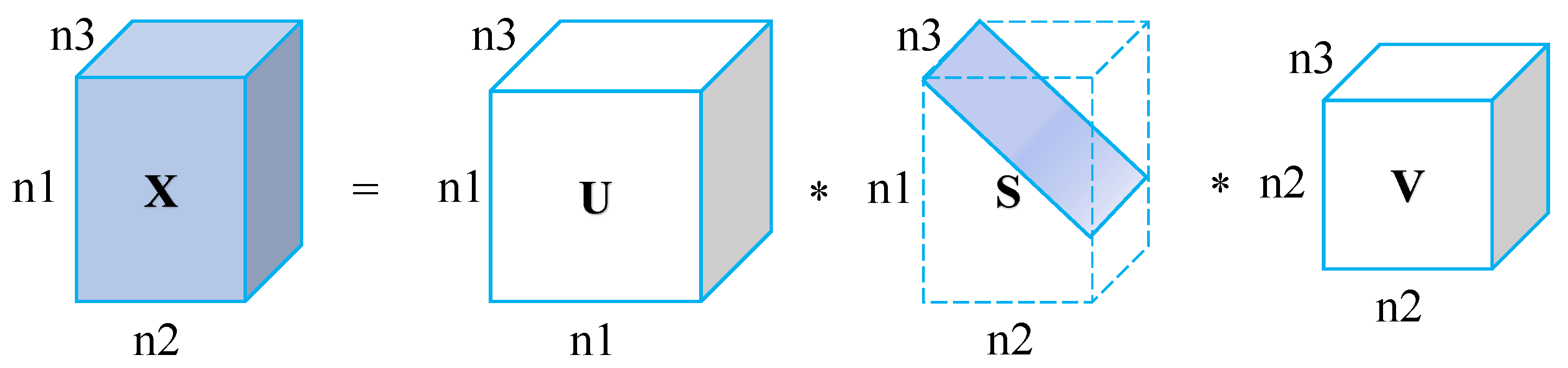
Compared with transforming each patch into a vector, the infrared patch-tensor model (IPT) introduced by Dai et al. [36] constructs the tensor model by directly stacking the patches, obtained via sliding a window from the top left to the bottom right over the image. Following this rationale, we establish the infrared patch-tensor model as follows:

$$\mathcal{D}=\mathcal{B}+\mathcal{T}+\mathcal{N}$$

(7)

where $\mathcal{D},\mathcal{B},\mathcal{T},\mathcal{N}\in {\mathbb{R}}^{m\times n\times k}$ represent the constructed image tensor, the decomposed background tensor, the target tensor, and the noise tensor, respectively. The construction method for the image tensor $\mathcal{D}$ is explained in a subsequent section. Using the low-rank sparse decomposition framework, we assume that the target tensor $\mathcal{T}$ exhibits sparsity, denoted as ${\parallel \mathcal{T}\parallel }_0<k$. Here, k is a constant that represents the level of sparsity, which is determined by the complexity of the infrared image. The noise tensor $\mathcal{N}$ is assumed to be additive white noise, expressed as ${\parallel \mathcal{N}\parallel }_F<\delta$. This leads to the constraint ${\parallel \mathcal{D}-\mathcal{B}-\mathcal{T}\parallel }_F<\delta$, where $\delta >0$.

The assumption of low-rankness for the background tensor $\mathcal{B}$ can be described as:

$$rank\left({\mathcal{B}}_{\left(1\right)}\right)\le r_1,rank\left({\mathcal{B}}_{\left(2\right)}\right)\le r_2,rank\left({\mathcal{B}}_{\left(3\right)}\right)\le r_3$$

(8)

where $rank\left({\mathcal{B}}_{\left(i\right)}\right),i=1,2,3$ denotes the rank of different slices of the background tensor $\mathcal{B}$. The constants $r_1,r_2$, and $r_3$ are positive and determined by the complexity of the image background. However, solving the rank by the L0 norm is challenging, and therefore the L1 norm is commonly used as an alternative approximation.

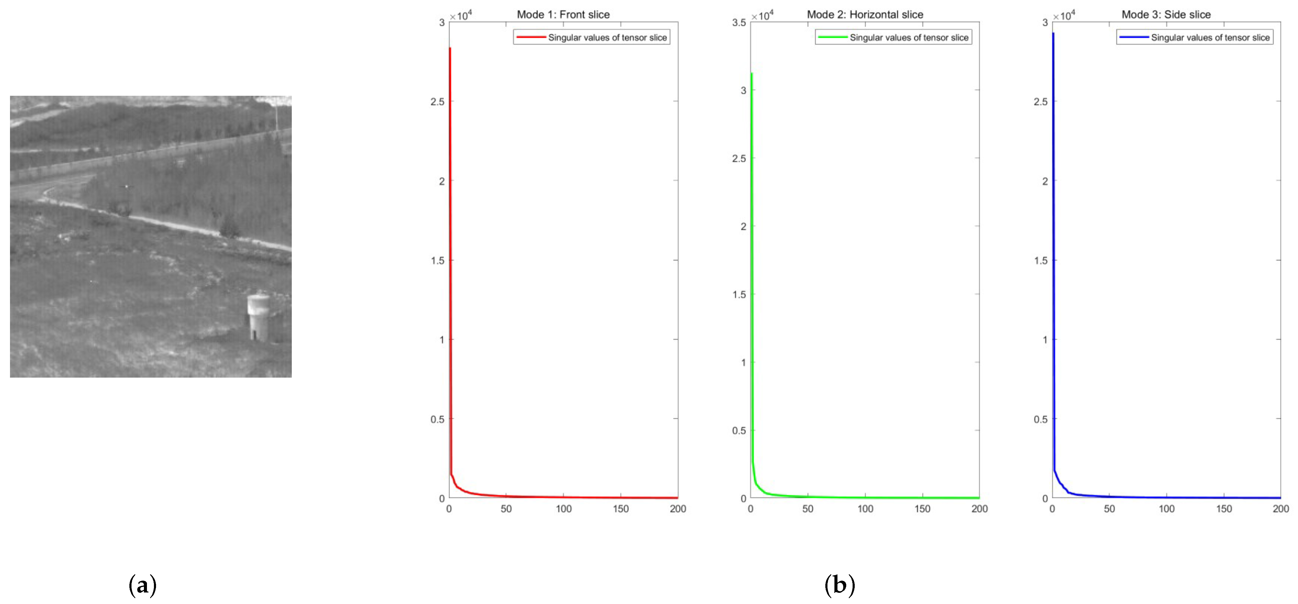
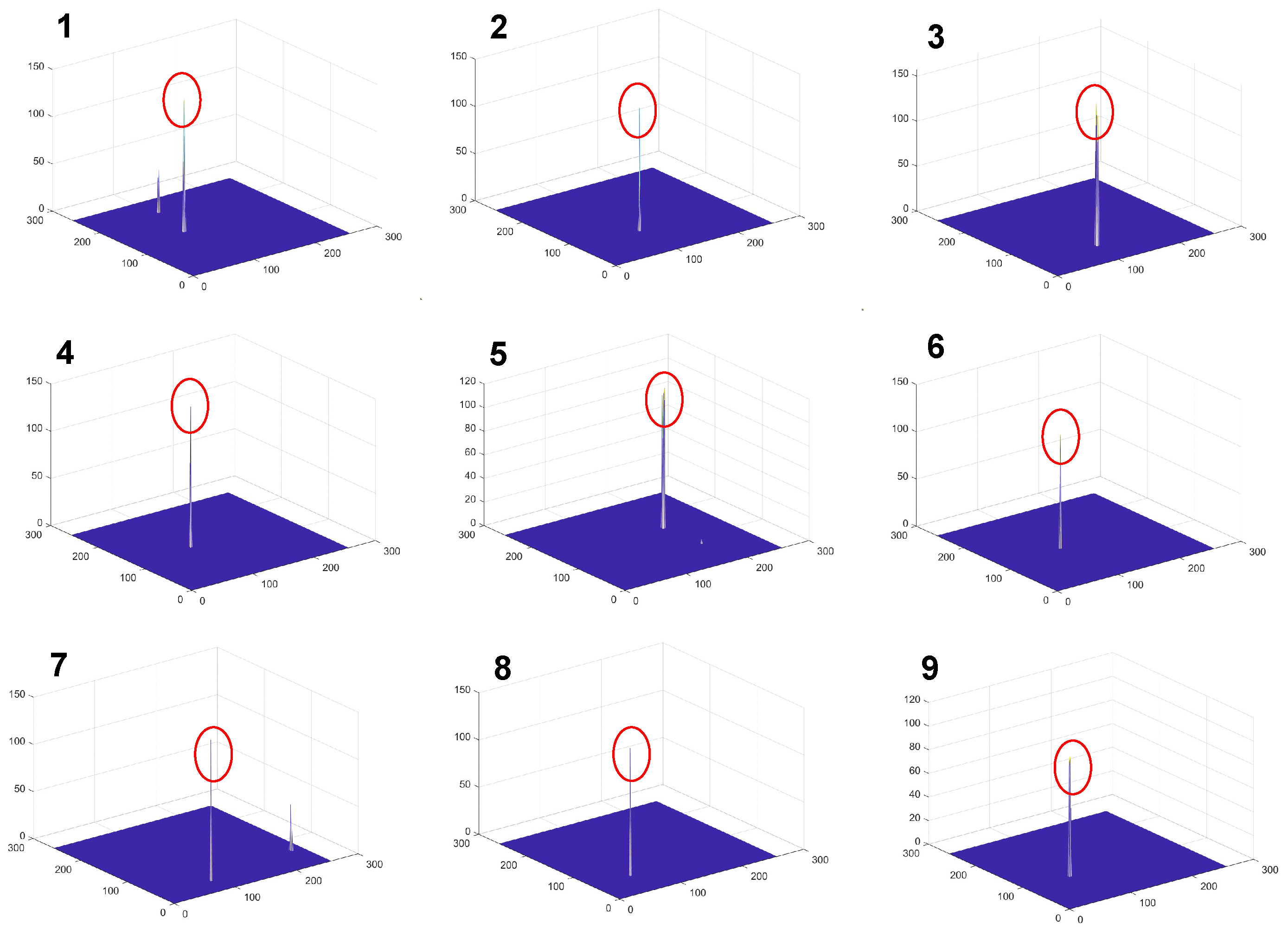
To examine the hypothesis of low-rankness, we unfold the raw tensor of the infrared image in three modes. This expansion enables us to analyze the variation of singular values for all modes. The results are presented in Figure 3. Notably, the singular values of the frontal slices, horizontal slices, and side slices demonstrate a pronounced decrease, which consistently aligns with the fundamental assumption of low-rank sparsity. Using the framework of low-rank sparse decomposition, we establish the following objective function:

$$\begin{array}{cc}\hfill \underset{B,T}{min}& rank\left(\mathcal{B}\right)+{\lambda \parallel \mathcal{T}\parallel }_1\hfill \\ \hfill s.t.& \mathcal{D}=\mathcal{B}+\mathcal{T}+{\mathcal{N},\parallel \mathcal{N}\parallel }_F<\delta \hfill \end{array}$$

(9)

where $\lambda$ is a compromising parameter that governs the trade-off between the target tensor and the background tensor. The L0 norm, which is computationally difficult to solve, is substituted with the L1 norm.

3.2. Spatial–Temporal Block-Matching Patch-Tensor Construction

Using a single-frame sliding window to acquire infrared patches and then constructing the tensor via these neighboring blocks is often ineffective in complex scenes. The SFBM model [31] attempts to improve the low-rankness of the tensor but still results in a significant number of false alarms and background residuals due to the lack of temporal information and the limitations of the matching criterion. The MFSTPT model [39] incorporates temporal information between frames through spatial–temporal sampling, but it still relies on the same neighborhood sliding window method as PSTNN [37] to obtain the tensor. Additionally, both the neighborhood sliding window method and matching block searching have redundancies, leading to a high number of repeated calculations in the subsequent iterative solution of the low-rank sparse decomposition, which results in generally low detection efficiency.

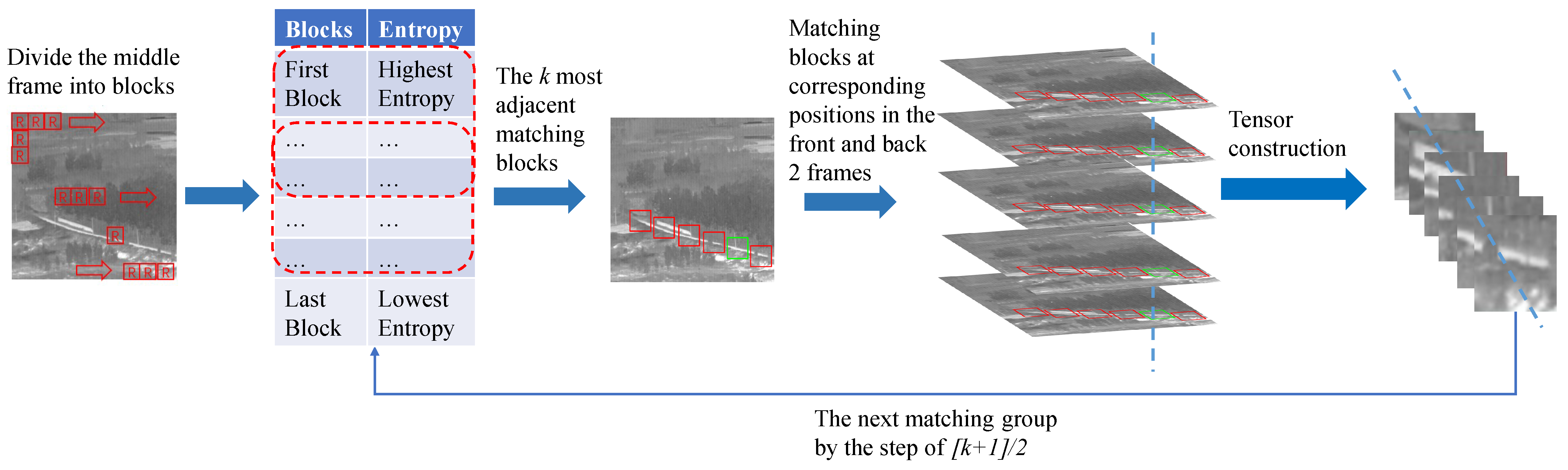
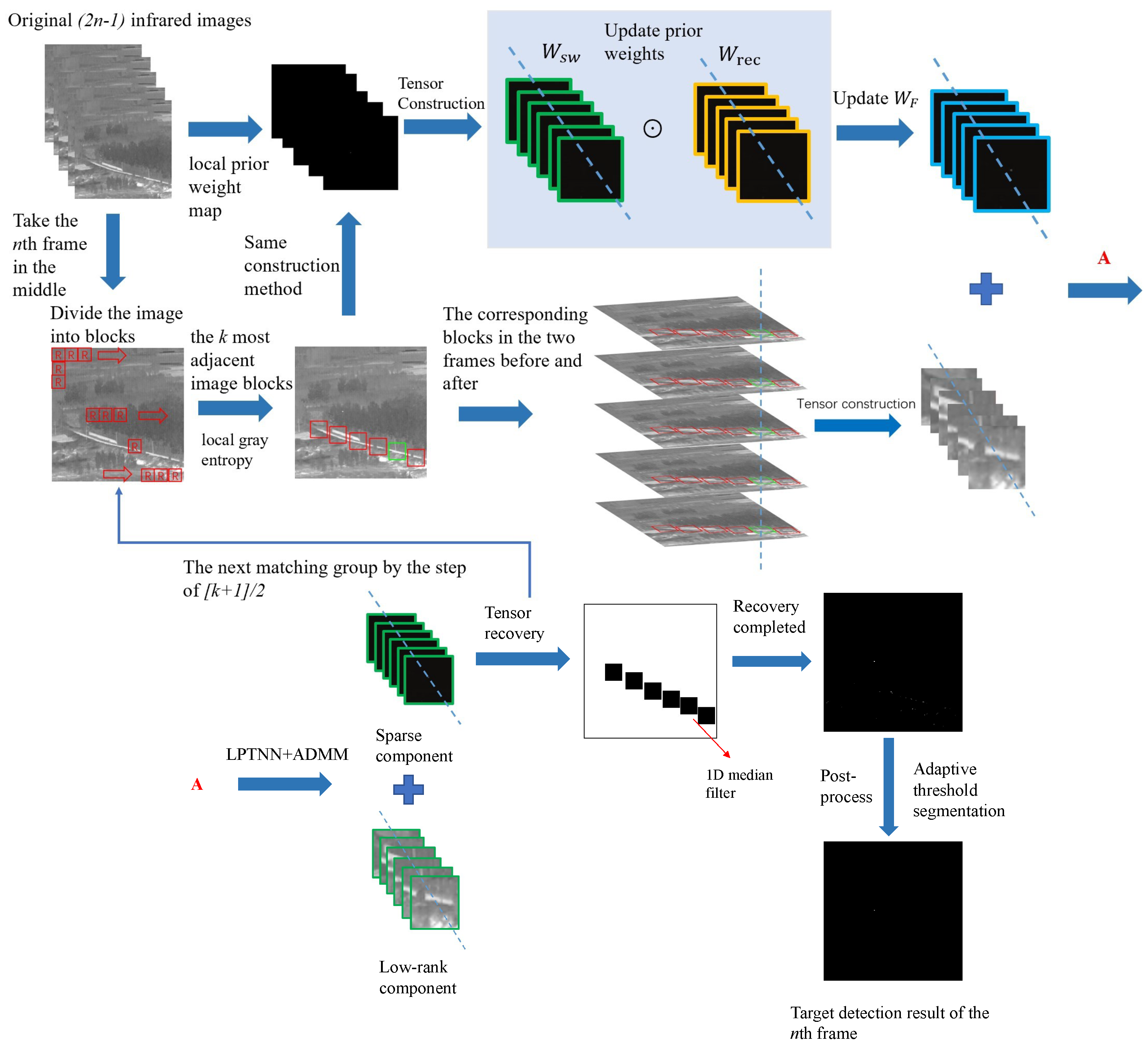
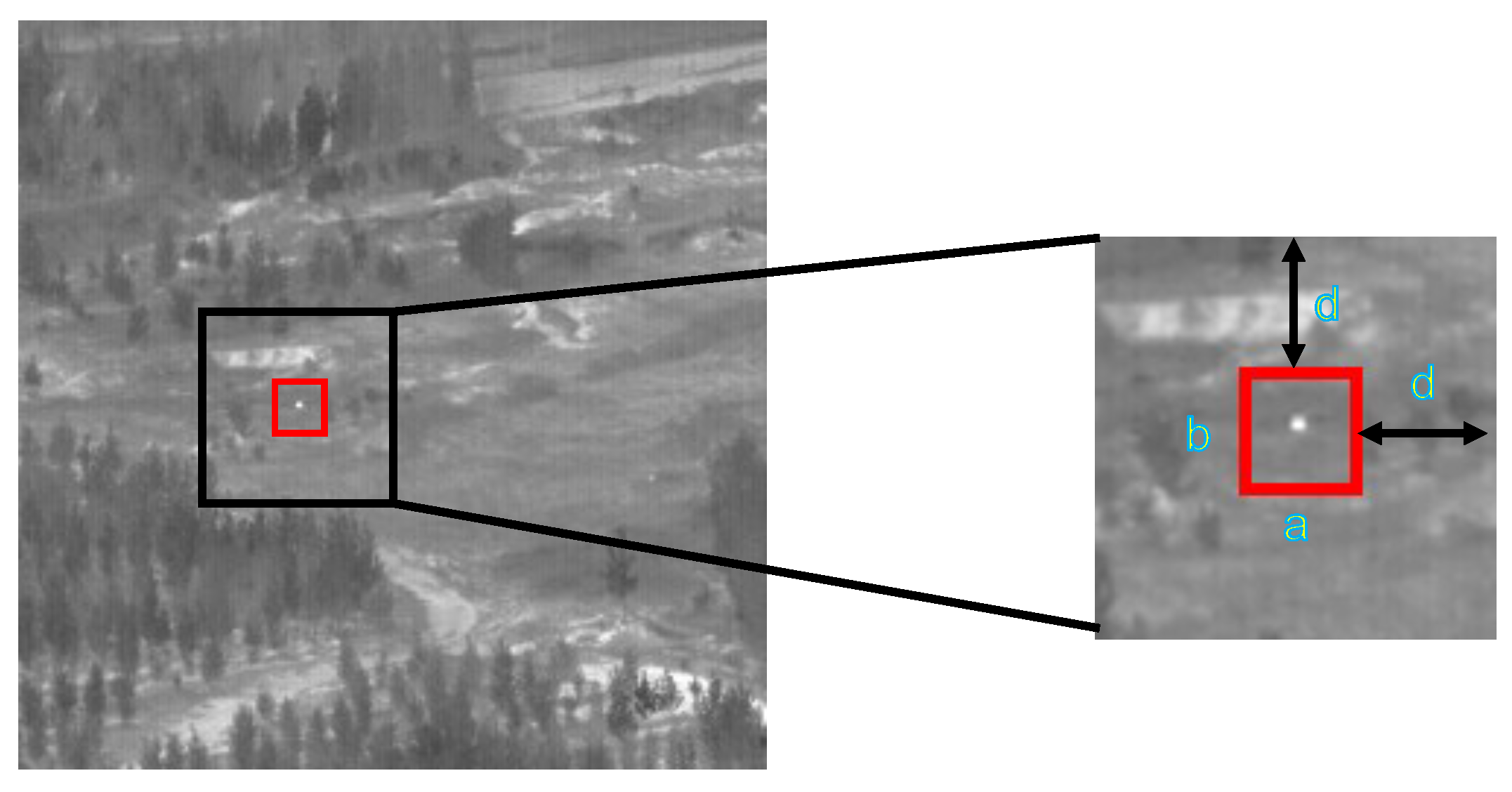
To address the aforementioned issues, we propose a spatial–temporal block-matching method to construct a low-rank tensor. First, the image is divided into multiple reference blocks, as shown in Figure 4. The matching values of each reference block are then computed. A matching group is formed by selecting the k most adjacent matching blocks. The current image frame is located in the middle of the image sequence. The green rectangle represents the current reference block, whereas the red border represents the matching block for this reference block. To detect the current image, we utilize its previous $(n-1)$ frames and subsequent $(n-1)$ frames, resulting in a total of $(2\times n-1)$ frames as the input model. Based on experimental testing, we set $n=3$ for the balance between detection accuracy and processing time. The middle frame image is divided into several reference blocks of a designated size. The local grayscale entropy value of each reference block is calculated as the matching value. These matching values are then sorted in descending order to obtain the top k blocks with the closest matching values. Together with the corresponding matching blocks in the preceding and subsequent frames, these k blocks form a matching group, which is used to construct a low-rank tensor. The value of k is determined by the ratio $\theta$ of the total number of matching blocks. The next matching group is selected from the sorted list of matching values in increments of $[k+1]/2$. This approach avoids the global searching of block acquirement, which reduces the times of decomposition iterations and thus can improve the detection efficiency.

3.3. Matching Criterion Based on the Local Grayscale Entropy

The SFBM model matches image blocks solely based on grayscale differences, thereby disregarding the spatial distribution and structural characteristics. Additionally, it also relies on a sliding window traversal approach for searching matching blocks, leading to low detection efficiency. Recently, local grayscale entropy has gained significant attention in the fields of small target detection and image enhancement [43,44,45]. To capture the spatial characteristics of the grayscale information in an image block, we establish a matching criterion based on the local grayscale entropy of the block. The pixel point of the statistical image, along with the surrounding neighborhood information, forms a new binary feature denoted as $(i,j)$, where i and j represent the grayscale values of the pixel and the corresponding neighborhood pixels, respectively. To further encompass the joint characteristics of the gray value at a pixel position and the gray distribution of its neighboring pixels, we define the probability of the occurrence of $f(i,j)$ in the image as $p_{ij}$:

$$p_{ij}=f(i,j)/(L\ast H)$$

(10)

where $f(i,j)$ denotes the number of occurrences of the binary feature $(i,j)$, and L and H signify the dimensions of the image. We can then calculate the local entropy of the given image block as follows:

$$S=-\sum _{i=0}^{255}\sum _{j=0}^{255}{p}_{ij}{log}_2{p}_{ij}$$

(11)

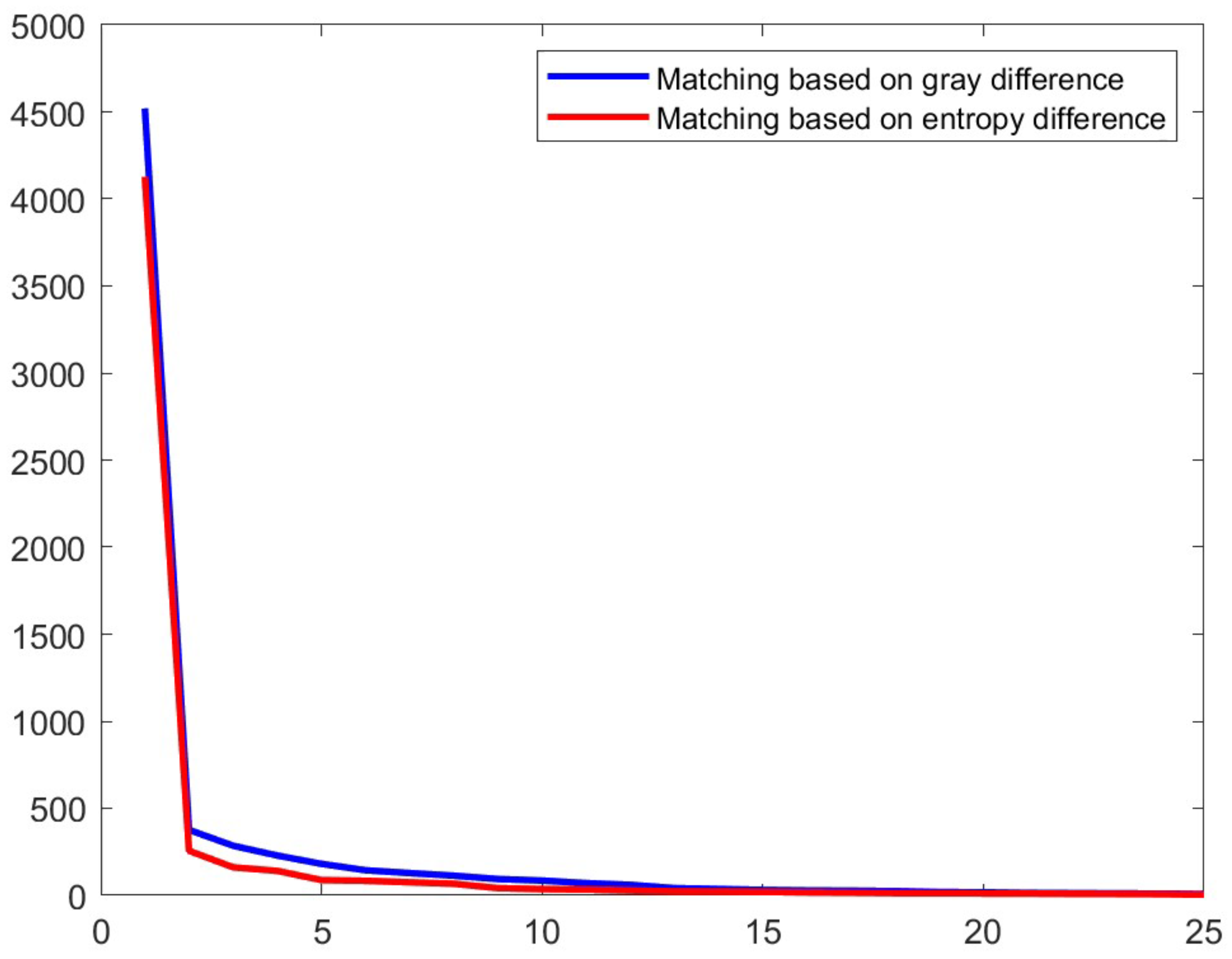
S represents the entropy value of the image block, and a higher similarity in the entropy value indicates better matching between the two image blocks, ultimately resulting in a more favorable low rank of the constructed tensor. Figure 5 demonstrates the singular-value curve of the tensor constructed from the image in Figure 3. It can be seen that the proposed method acquires a faster-decreasing curve compared to the grayscale difference employed in the SFBM model.

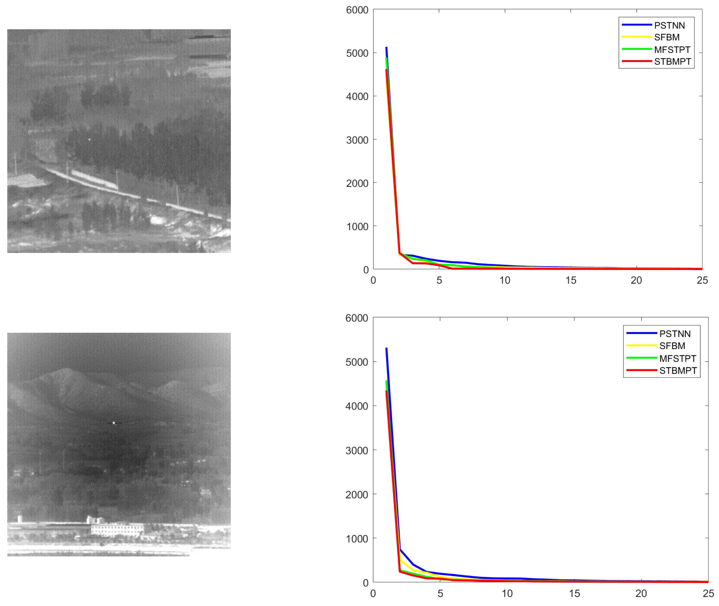
Moreover, we compare the PSTNN, SFBM, and MFSTPT models with the proposed STBMPT model for the construction of a low-rank tensor/matrix in two different infrared image sequences, and the corresponding singular-value curves are depicted in Figure 6. The results demonstrate that the proposed tensor construction method displays the fastest decline in singular values and achieves the best low-rank properties.

3.4. Local Prior Information

False alarms in infrared small moving target detection frequently arise from strong edges and corner points in intricate backgrounds, which often become the background residuals and subsequently impact the accuracy. Therefore, it is necessary to compute local priors to suppress the pixels associated with strong edges and bright corner points before iteratively solving the model. Gao et al. [46] proposed a method to distinguish edges from corner points by calculating the eigenvalues (${\lambda }_1,{\lambda }_2$) of the structure tensor of pixels:

$$J_{\rho }=K_{\rho }·(\Delta D_{\rho }\otimes \Delta D_{\rho })=\left(\begin{array}{cc}{J}_{11}& J_{12}\\ J_{21}& J_{22}\end{array}\right)=\left(\begin{array}{cc}{K}_{\rho }·I_x^2& K_{\rho }·I_x{I}_y\\ K_{\rho }·I_x{I}_y& K_{\rho }·I_y^2\end{array}\right)$$

(12)

$$\begin{array}{c}\hfill {\lambda }_1=\frac{1}{2}\left(J_{11}+J_{22}+\sqrt{{(J_{22}-J_{11})}^2+4J_{12}^2}\right)\\ \hfill {\lambda }_2=\frac{1}{2}\left(J_{11}-J_{22}+\sqrt{{(J_{22}-J_{11})}^2+4J_{12}^2}\right)\end{array}$$

(13)

where $\Delta$ is the gradient operator, and $I_x$ and $I_y$ are the derivatives with respect to the x- and y-directions. $K_{\rho }$ represents a Gaussian kernel function with variance $\rho$, and ⊗ denotes the Kronecker product. Gao et al. demonstrated that when ${\lambda }_1\gg {\lambda }_2\approx 0$, the pixel corresponds to a corner point. On the other hand, when ${\lambda }_1\ge {\lambda }_2\approx 0$, the pixel is associated with an edge. Finally, when ${\lambda }_1\approx {\lambda }_2\approx 0$, the pixel belongs to a smooth background region.

The local prior weight used in RIPT [36] is as follows:

$$E(x,y)={\lambda }_1-{\lambda }_2$$

(14)

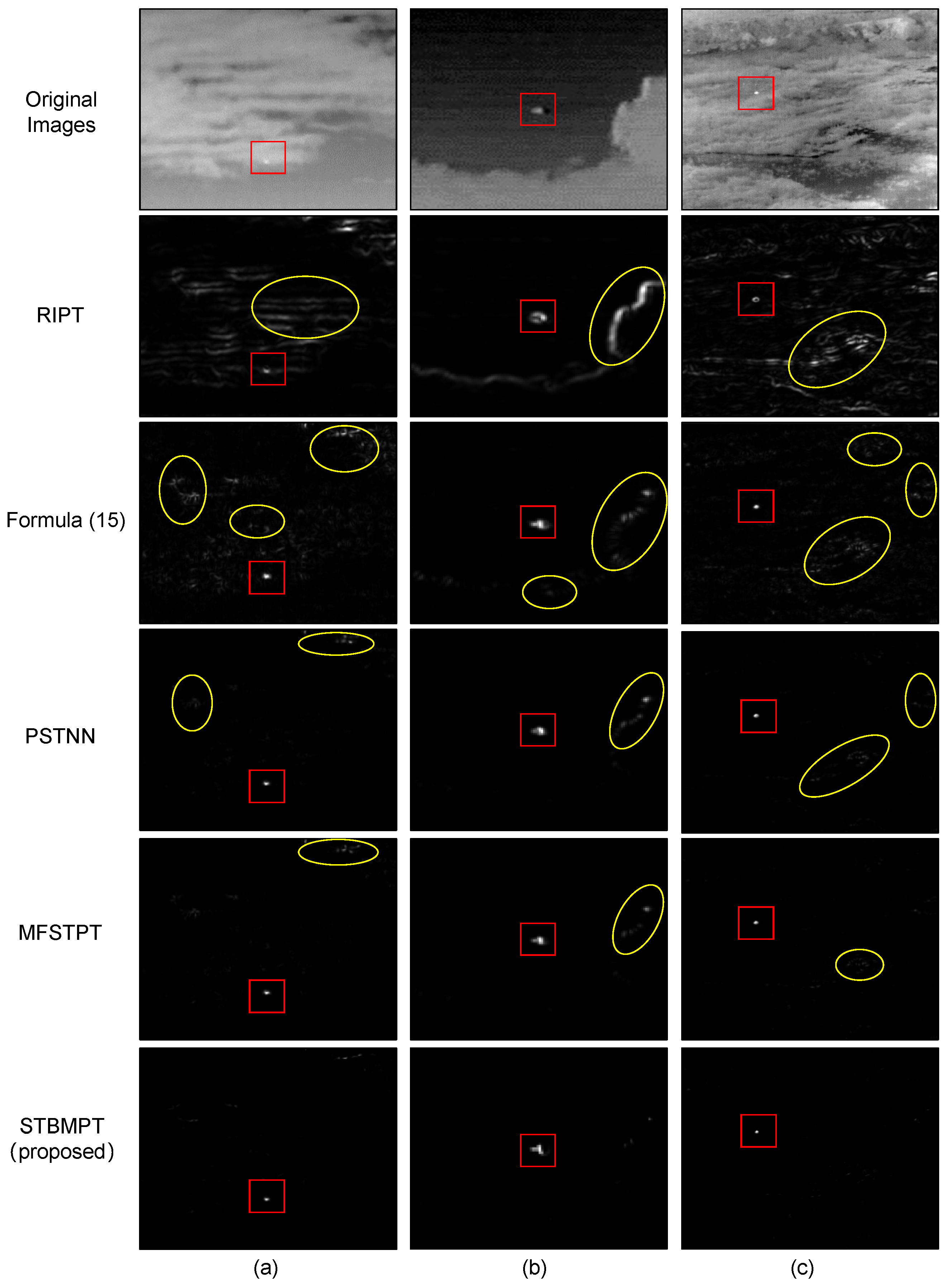
where $(x,y)$ denotes the pixel location. It can be observed in the second row in Figure 7 that RIPT only evaluates the edges, which may result in more edge residues in the detection outcomes, thereby affecting the results. The corner-point weighting function proposed by Brown et al. [47] is as follows:

$$C=w_{cs}(x,y)=\frac{det\left(ST\right(x,y\left)\right)}{\mathrm{tr}\left(ST\right(x,y\left)\right)}=\frac{{\lambda }_1·{\lambda }_2}{{\lambda }_1+{\lambda }_2}$$

(15)

where $w_{cs}(x,y)$ is half of the harmonic mean of the eigenvalues; $det(·)$ and $tr(·)$ are the determinant and trace of the matrix, respectively; and $ST(·)$ is the structure tensor. Using Formula (15) as the prior weights leads to residual corner-point elements, contributing to a significant amount of point noise in the detection results, as shown in the third row in Figure 7.

The PSTNN model [37] employs the maximum value of the eigenvalues instead of the difference as the edge weight function and multiplies it with Formula (15) to obtain the prior weights, as shown in Formula (16). Partly suppressing the strong edges, this method still lacks sufficient suppression of strong corner pixels, as shown in the fourth row in Figure 7.

$$W_p(x,y)=C\odot E=max({\lambda }_1,{\lambda }_2)\odot \frac{{\lambda }_1·{\lambda }_2}{{\lambda }_1+{\lambda }_2}$$

(16)

The MFSTPT model [39] computes the prior weight in the form of a weighted geometric average. This formula combines the edge weighting function presented in Formula (14) and the corner-point weighting function presented in Formula (15), as indicated in Formula (17):

$$W_c(x,y)=\sqrt[n]{C^p·E^q}$$

(17)

However, as depicted in the fifth row in Figure 7, the background residuals still cannot be eliminated when there are significant fluctuations near the edges.

To address the above issues, in combination with the previously mentioned laws of the structure tensor (${\lambda }_1$ and ${\lambda }_2$), we introduce a new local prior-weight calculation method inspired by the Frangi filtering method [48]. We begin by defining two indicators that depict the shape of the pixels:

$$R(x,y)=\frac{\left|{\lambda }_1\right|}{\left|{\lambda }_2\right|}$$

(18)

$$S(x,y)=\sqrt{{\lambda }_1^2+{\lambda }_2^2}$$

(19)

Here, ${\lambda }_1$ and ${\lambda }_2$ are the two eigenvalues, and $|{\lambda }_2|\ge |{\lambda }_1|$. In the case of a speckled shape, the two eigenvalues are close to each other, resulting in a larger R-value. Conversely, when the shape is expressed as an edge, the difference between the two eigenvalues is larger, leading to a smaller R-value. Furthermore, when the pixels belong to the background, the eigenvalues are both smaller, resulting in a smaller S-value. On the contrary, the S-value is larger if there is at least one larger eigenvalue present. Therefore, we establish the local prior weights as:

$$W_P(x,y)=exp\left(-\frac{R^2}{2{\beta }^2}\right)·\left(1-exp\left(-\frac{S^2}{2c^2}\right)\right)$$

(20)

Here, $W_P(x,y)$ represents the local prior weights of the pixel positions in the image. The parameters $\beta$ and c are used to adjust the sensitivity of the edge and corner-point weights. In this paper, $\beta$ is set at 2 and the value of c is set at half of the maximum S-value among all pixels. The weights are then normalized as:

$${\mathcal{W}}_P=\frac{{\mathcal{W}}_P-w_{\min }}{w_{\max }-w_{\min }}$$

(21)

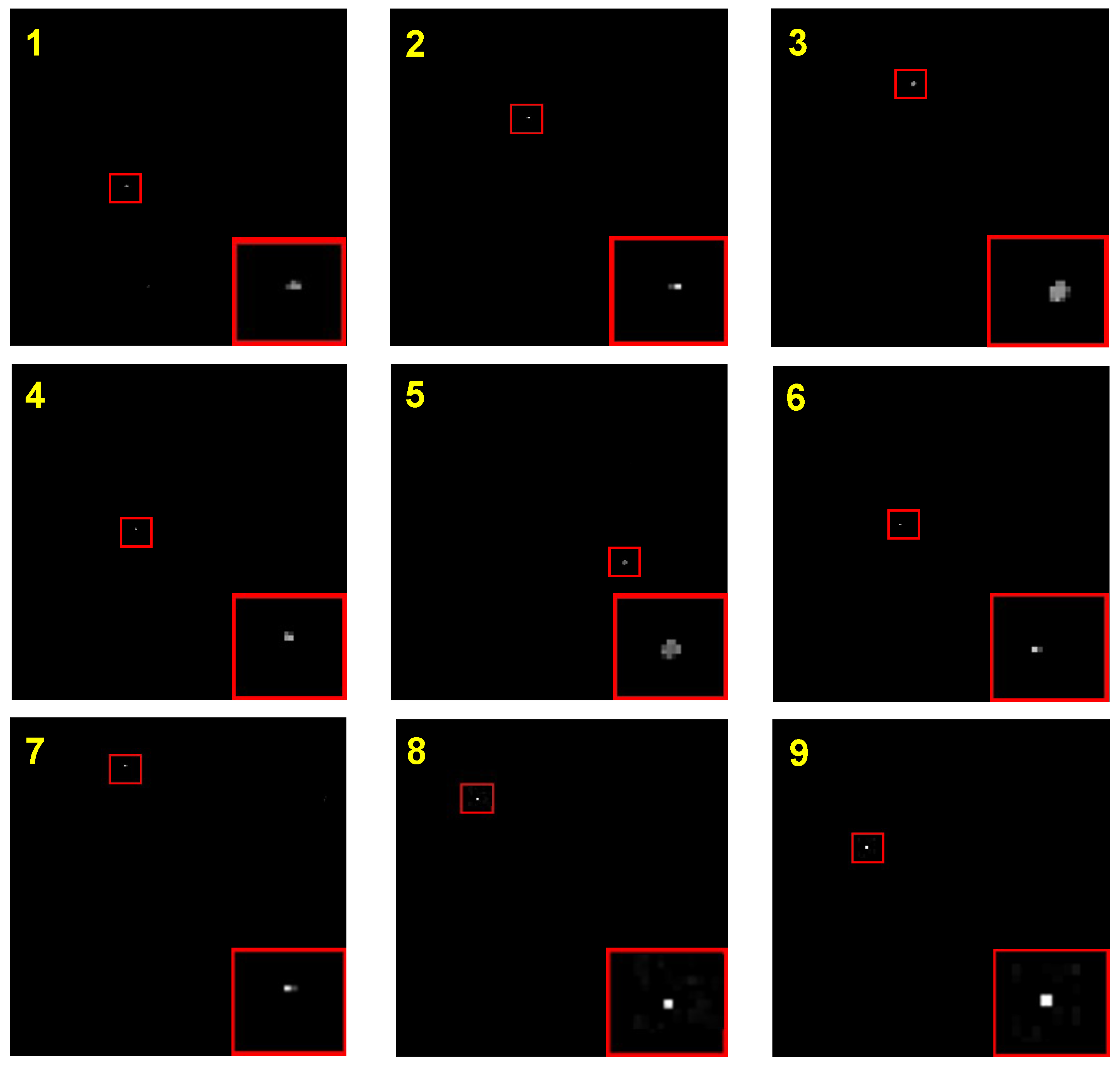
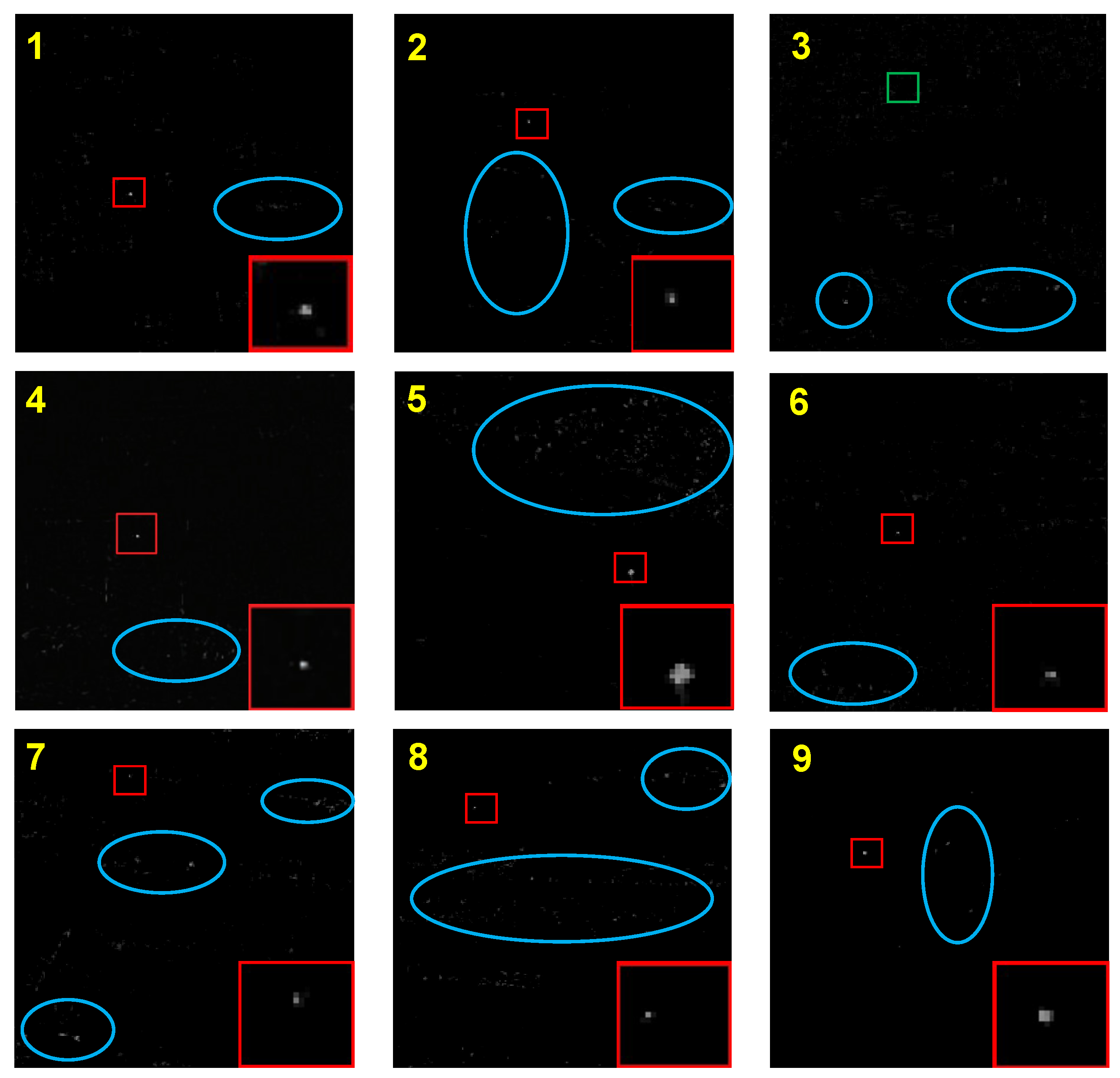
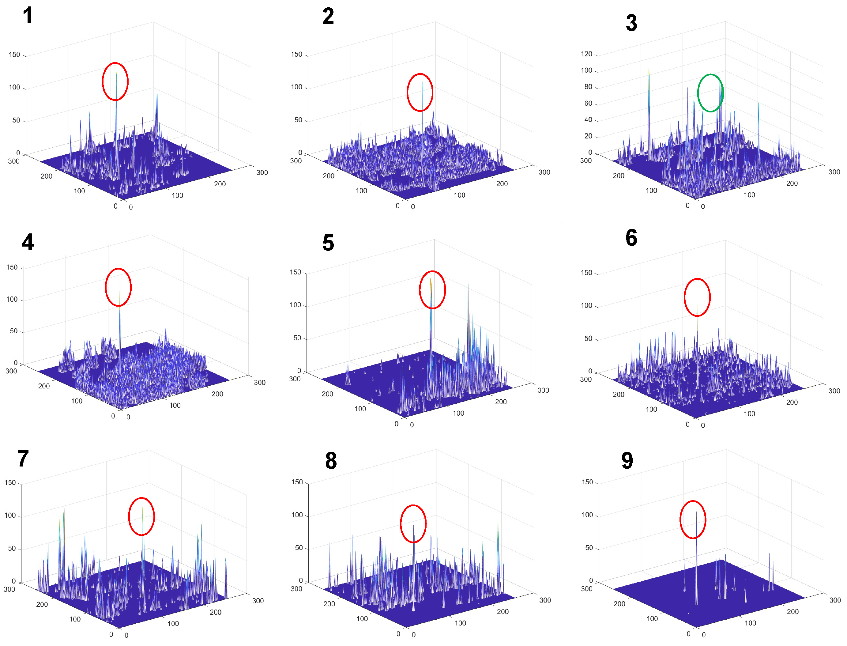
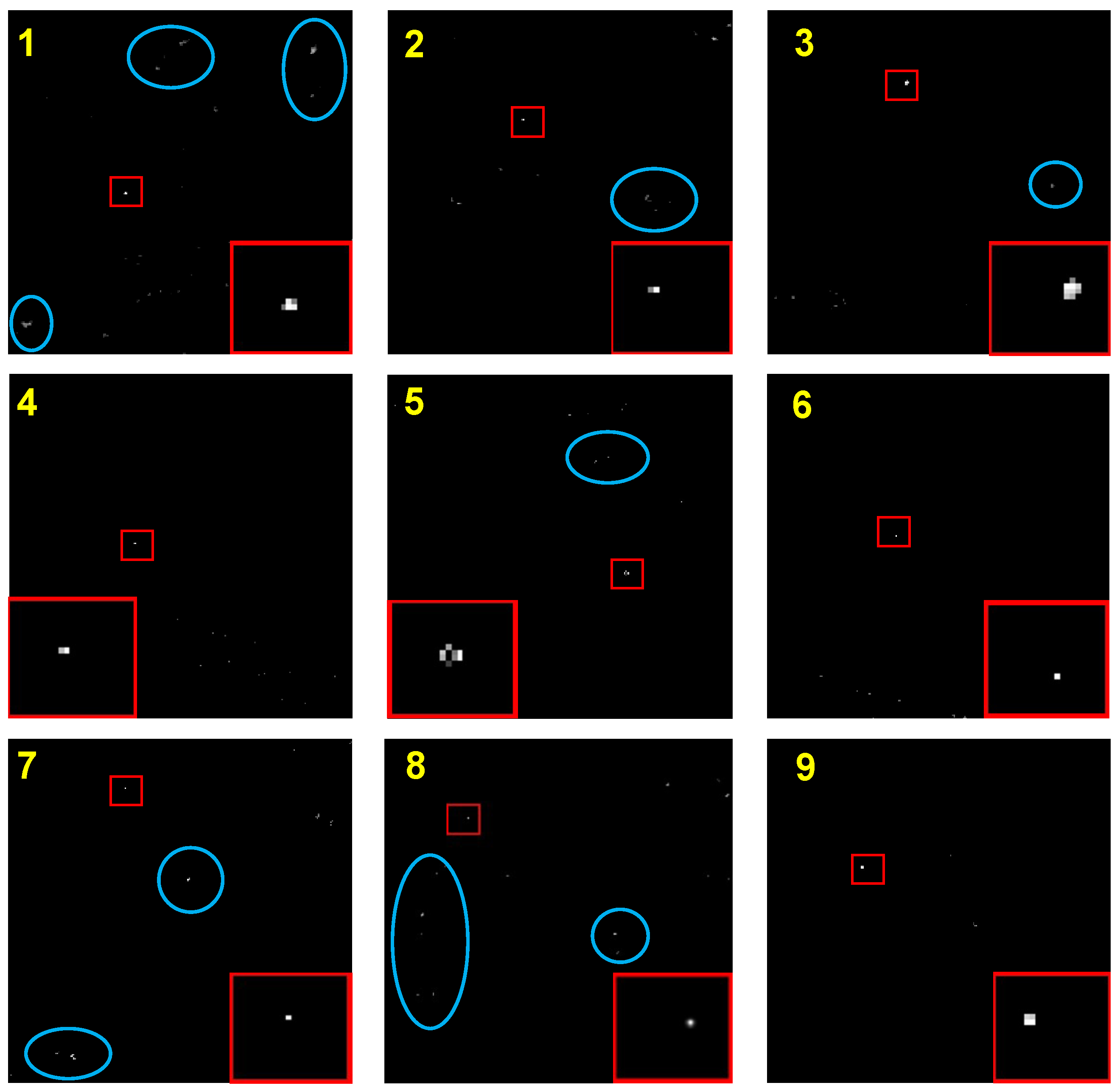
where $w_{\min }$ and $w_{\max }$ represent the minimum and maximum values in $W_P$, respectively. The prior weights proposed in this paper allocate appropriate weights to the background edges and corner points, effectively suppressing strong edges and bright corner points while highlighting the target. To compare the impacts of different prior weights, we employ the aforementioned state-of-the-art prior weights to calculate the local weight maps for three common infrared images, which are presented in Figure 7. The targets are enclosed within red boxes, whereas the residual background is enclosed within yellow elliptical boxes. It is evident that the proposed prior weights offer superior results compared to other models. Although there is a slight shrinkage of the target, the background residuals are significantly suppressed regardless of whether it is a complex or smooth background.

3.5. Sparsity Constraints and Rank Approximation

For the L1 parametric sparsity constraint on the target component $\mathcal{T}$ in Formula (9), the widely used sparsity-enhanced weighting scheme is employed to minimize the L1 norm [49]:

$${\mathcal{W}}_{\mathrm{SW}}^{(k+1)}=\frac{p}{\left|{\mathcal{T}}^k\right|+ϵ}$$

(22)

where p represents a non-negative constant, $ϵ$ is a small positive number introduced to prevent division by zero, and k represents the number of iterations. Combining the sparse weights in Formula (22) and the prior weights in Formula (21), the target weight matrix is constructed as follows:

$$\mathcal{W}={\mathcal{W}}_{\mathrm{SW}}\odot {\mathcal{W}}_{\mathrm{rec}}$$

(23)

where $W_{rec}$ is the reciprocal of the corresponding element of $W_P$ and ⊙ denotes the Hadamard product.

For the low-rank constraint of the background component $\mathcal{B}$ in Formula (9), the approximation of the tensor rank is a crucial issue. To address this, we adopt the rank approximation method based on the Laplace operator used in the MFSTPT model [39]. This method, known as the Laplace patch-tensor nuclear norm (LPTNN), is used to approximate the background tensor rank as shown in Formula (24). Compared to other methods, the Laplace operator is able to assign automatic weights to singular values, resulting in a closer approximation to the background tensor rank.

$${\parallel \mathcal{X}\parallel }_{\mathrm{LPTNN}}=\sum _{i=1}^{n^3}\sum _{j=1}^p\varphi \left({\sigma }_j\left({\overline{X}}^i\right)\right)=\sum _{i=1}^{n^3}\sum _{j=1}^p\left(1-e^{-{\sigma }_j\left({\overline{X}}^i\right)/\gamma }\right)$$

(24)

where ${\sigma }_j\left({\overline{X}}^i\right)$ represents the singular value of the ith frontal slice, p is the number of singular values, and $\gamma$ is a small positive number. As a result, the proposed solution model is updated in Formula (25):

$$\begin{array}{cc}\hfill \underset{B,T}{min}& {∥\mathcal{B}∥}_{LPTNN}+\lambda {∥\mathcal{W}\odot \mathcal{T}∥}_1\hfill \\ \hfill s.t.& \mathcal{D}=\mathcal{B}+\mathcal{T}+{\mathcal{N},\parallel \mathcal{N}\parallel }_F<\delta \hfill \end{array}$$

(25)

3.6. Optimization and Solution of the Proposed Model

The alternating direction method of multipliers (ADMM) method has been widely recognized for its fast convergence and high solution accuracy in solving problems involving low-rank sparse decomposition [50]. We employ the ADMM method to solve the model in Formula (25) through the following procedure.

Firstly, we express the model to be solved in the form of an augmented Lagrangian function, given by:

$$L_{\mu }(\mathcal{B},\mathcal{T},\mathcal{W},\mathcal{Y})={∥\mathcal{B}∥}_{\mathrm{LPTNN}}+\lambda {∥\mathcal{W}\odot \mathcal{T}∥}_1+〈\mathcal{Y},\mathcal{B}+\mathcal{T}-\mathcal{D}〉+\frac{\mu }{2}{∥\mathcal{B}+\mathcal{T}-\mathcal{D}∥}_F^2$$

(26)

where $\mathcal{Y}$ is a Lagrange multiplier, $\mu$ is a penalty factor greater than 0, $〈·〉$ denotes the inner product, and ${\parallel \mathcal{N}\parallel }_F$ is replaced by ${\parallel \mathcal{B}+\mathcal{T}-\mathcal{D}\parallel }_F$ according to the constraints in Formula (25). To solve for $\mathcal{B}$ and $\mathcal{T}$, we solve for the other variable while keeping one variable fixed. As a result, the problem in Formula (26) can be decomposed into two subproblems:

$${\mathcal{T}}^{k+1}=arg\underset{\mathcal{T}}{min}\lambda {∥{\mathcal{W}}^k\odot \mathcal{T}∥}_1+\frac{{\mu }^k}{2}{∥{\mathcal{B}}^k+\mathcal{T}-\mathcal{D}+\frac{{\mathcal{Y}}^k}{{\mu }^k}∥}_F^2$$

(27)

$${\mathcal{B}}^{k+1}=arg\underset{\mathcal{B}}{min}{∥\mathcal{B}∥}_{\mathrm{LPTNN}}+\frac{{\mu }^k}{2}{∥\mathcal{B}+{\mathcal{T}}^{k+1}-\mathcal{D}+\frac{{\mathcal{Y}}^k}{{\mu }^k}∥}_F^2$$

(28)

• The first subproblem can be effectively resolved using a soft thresholding optimization algorithm [51]. By applying thresholding to the tensor elements, the solution to Subproblem (27) of the target tensor can be obtained as follows:

  $${\mathcal{T}}^{k+1}=S_{\frac{\lambda {\mathcal{W}}^k}{{\mu }^k}}\left(\mathcal{D}-{\mathcal{B}}^k-\frac{{\mathcal{Y}}^k}{{\mu }^k}\right)$$

  (29)

  where $S_{\tau }\left(x\right)$ is the thresholding operator:

  $$S_{\tau }\left(x\right)=\mathrm{sign}\left(x\right)·max\left(\right|x|-\tau ,0)$$

  (30)
• For the subproblem in Formula (28), the task of solving the background tensor is initially conceptualized as the following optimization problem:

  $$arg\underset{\mathcal{X}}{min}{∥\mathcal{X}∥}_{\mathrm{LPTNN}}+\frac{\beta }{2}{∥\mathcal{X}-\mathcal{Z}∥}_F^2$$

  (31)

  In fact, we can calculate the non-convex rank of the LPTNN substitution by combining all the front slices of the tensor in the Fourier transform domain along $X(:,:,1,\cdots ,n3)$. This transformation converts the problem into an optimization problem for the sum of the singular values of $n_3$ matrices:

  $$arg\underset{{\overline{X}}^{\left(g\right)}}{min}\sum _{i=1}^{n_3}\varphi \left({\sigma }_i\left({\overline{X}}^{\left(g\right)}\right)\right)+\frac{\beta }{2}{∥{\overline{X}}^{\left(g\right)}-{\overline{Z}}^{\left(g\right)}∥}_F^2$$

  (32)

  where ${\overline{X}}^{\left(g\right)},{\overline{Z}}^{\left(g\right)}\in {\mathbb{R}}^{n_1\times n_2},g=1,2,\dots ,n_3$ are two-dimensional frontal slices. To address Problem (32), the generalized weighted singular-value threshold operator [52] is employed:

  $${\overline{X}}^{\left(g\right)}={\overline{U}}^{\left(g\right)}·{\overline{D}}^{\left(g\right)}·{{\overline{V}}^{\left(g\right)}}^H$$

  (33)

  $${\overline{D}}_{\frac{\Delta \varphi }{\beta }}^{\left(g\right)}=max\left(\left({\overline{S}}^{\left(g\right)}(i,i)-\frac{\Delta \varphi \left({\sigma }_i^{k,g}\right)}{\beta }\right),0\right)$$

  (34)

  where

  $${\overline{Z}}^{\left(g\right)}={\overline{U}}^{\left(g\right)}·{\overline{S}}^{\left(g\right)}·{{\overline{V}}^{\left(g\right)}}^H$$

  (35)

  $$\Delta \varphi \left({\sigma }_i^{k,g}\right)=\frac{1}{\epsilon }exp\left(-\frac{{\sigma }_i^{k,g}}{\epsilon }\right)$$

  (36)

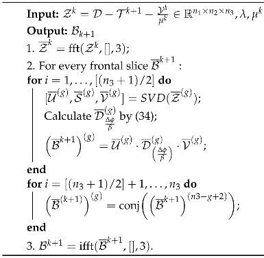
  An inverse Fourier transform of the result yields X. Therefore, the background tensor in Problem (28) can be resolved. The algorithm’s flow is illustrated below in Algorithm 2.

Algorithm 2:Solution for the background tensor problem (28)

    $\mathcal{Y}$ and $\mu$ are updated based on the following formulas:

$${\mathcal{Y}}^{k+1}={\mathcal{Y}}^k+{\mu }^k(\mathcal{D}-{\mathcal{B}}^{k+1}-{\mathcal{T}}^{k+1})$$

(37)

$${\mu }^{k+1}=\rho {\mu }^k$$

(38)

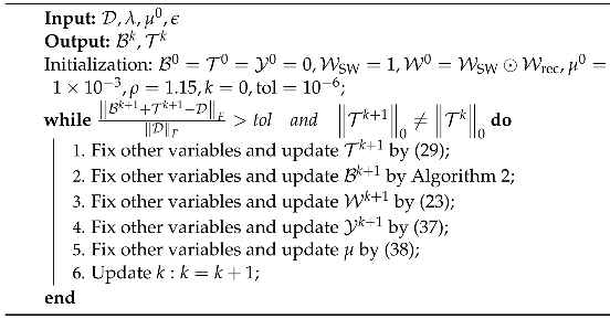
Algorithm 3 shows the complete process of utilizing the ADMM method to optimize and solve the proposed model. The algorithm’s post-processing step applies a simple threshold segmentation to the target components. The threshold value is determined as $mean+q\ast s$, where $mean$ represents the average grayscale value of the entire image, s stands for the standard deviation of the image’s grayscale, and q is a constant.

Algorithm 3:Solution of the proposed model.

3.7. The Flowchart of the Proposed Model

Figure 8 illustrates the complete process of the proposed STBMPT model.

• The input consists of an image sequence, where five consecutive frames are taken;
• The local prior-weight map is constructed using Formula (23);
• The tensor is then constructed by partitioning each frame into image blocks of a certain size. The local gray entropy of each image block is calculated and sorted. The tensor $\mathcal{X}$ is constructed by considering the k most adjacent image blocks according to the step of $[k+1]/2$. The corresponding image blocks in the two frames before and after are grouped;
• Using the ADMM algorithm based on the LPTNN constraint, the matching block tensor $\mathcal{D}$ and prior-weight tensor $\mathcal{W}$ are decomposed into a low-rank background tensor $\mathcal{B}$ and a sparse target tensor $\mathcal{T}$;
• The tensor recovery process involves placing each frontal slice of the sparse target tensor $\mathcal{T}$ and the low-rank background tensor $\mathcal{B}$ back in their original positions in the image. A one-dimensional median filter is then applied to the overlapping pixel positions;
• Finally, an adaptive threshold segmentation is performed on the recovered sparse target result map to obtain the final target image.

4. Experiments and Results

In this section, we conduct experimental validation of the proposed model, which consists of an introduction to the evaluation metrics, a description of the dataset used in the experiment, parameter analysis, a quantitative evaluation of background suppression and target detection accuracy, an evaluation of the detection efficiency, and a comprehensive comparison of the experimental results with those of current state-of-the-art infrared small moving target detection methods.

4.1. Evaluation Metrics

The proposed method is assessed through the evaluation metrics commonly utilized in this field, and the target with its adjacent region is illustrated in Figure 9. The dimensions of the target region are denoted as $a\ast b$, whereas the size of the surrounding background region is represented as $(a+2d)\ast (b+2d)$.

The evaluation metrics utilized include the following:

(1)

The signal-to-clutter ratio gain (SCRG) can evaluate the suppression of clutter and enhancement of the target, which comes from the signal-to-clutter ratio (SCR) and is computed as follows:

$$SCR=\frac{|{\mu }_t-{\mu }_b|}{{\sigma }_b}$$

(39)

where ${\mu }_t$ and ${\mu }_b$ denote the grayscale mean of the target region and the neighborhood background region, and ${\sigma }_b$ represents the grayscale standard deviation of the neighborhood background region, as shown in Figure 9. As a result, the SCRG is defined as:

$$SCRG=\frac{SC{R}_{out}}{SC{R}_{in}}$$

(40)

where $SC{R}_{out}$ represents the SCR value of the output target image, and $SC{R}_{in}$ represents the SCR value of the original input image.

(2)

The background suppression factor (BSF) [53] can be utilized to assess the extent of background suppression, which is determined using the following equation:

$$BSF=\frac{{\delta }_{in}}{{\delta }_{out}}$$

(41)

where ${\delta }_{in}$ represents the standard deviation of the background area in the input image, and ${\delta }_{out}$ represents the standard deviation of the background area in the output image.

(3)

The detection rate $P_d$ and false alarm rate $F_a$ are utilized to evaluate the performance of the algorithm and can be calculated as:

$$P_d=\frac{DT}{AT}$$

(42)

where $DT$ is the number of detected targets, and $AT$ is the actual number of targets in the original image sequence. The false alarm rate is determined as follows:

$$F_a=\frac{FP}{NP}$$

(43)

where $FP$ is the number of pixels in the false alarm region, and $NP$ is the total number of pixels in the image sequence. The detection performance of the algorithm can be visualized by plotting a receiver operating characteristic (ROC) curve. This curve represents the trade-off between the detection rate (horizontal coordinate) and the false alarm rate (vertical coordinate). The area enclosed by the ROC curve and the coordinate axis is the AUC value, which stands for the area under the curve. A higher AUC value indicates a better performance of the target detection algorithm.

4.2. Dataset Description

The experiments were conducted on a dataset consisting of real infrared image sequences of small moving aircraft targets with a ground/air background [54]. This dataset specifically focuses on airborne infrared targets and includes various scenes such as the sky and ground features in complex situations. The target locations in the dataset are marked by red boxes, as shown in Figure 10. To evaluate the performance of the proposed method, five representative scenes were selected as the test sequence.

Table 4. Description of the five sequences.

Sequence	Total Frame	Average SCR	Description
Data 2	399	5.11	Near to far, single moving target, ground background
Data 4	399	6.07	Far to near, single moving target, ground background
Data 7	399	1.51	Near and far, single small moving target, ground background, interference from strong edges and bright points in the background
Data 8	398	3.42	Faint and small moving target, ground background
Data 9	399	3.32	Single moving target, complex background in air-to-ground scenarios

provides detailed descriptions of these five data segments. All of the experiments were implemented using Matlab R2021a on Windows 11, based on an 11th Gen Intel Core i5-11320H 3.20 GHz CPU with 16G of RAM.

4.3. Parameter Analysis

To improve the performance of our proposed model with real datasets, it is crucial to set appropriate parameters through experimental analysis. Essential parameters, including the compromising parameter $\lambda$, penalty factor $\mu$, block size, and matching ratio $\theta$, have a significant impact on the robustness of the model in different scenes. In Figure 11, we present the ROC curves for the five real infrared sequences in Table 4, demonstrating the performance variation under different model parameters while keeping the others fixed. The rows in the table correspond to different parameters arranged in the same sequence, whereas the columns represent the results of a particular parameter across different sequences. It is important to note that solely optimizing one parameter while keeping the others constant may not result in globally optimal outcomes.

4.3.1. Compromising Parameter

The parameter $\lambda$ serves as a compromise between the background tensor $\mathcal{B}$ and the target tensor $\mathcal{T}$, as presented in Formula (25). Previous studies [34,36] were consulted to determine the value of $\lambda$:

$$\lambda =\frac{L}{\sqrt{max(n1,n2)·n3}}$$

(44)

By adjusting the values of L, we tested the impact of the compromising parameter $\lambda$ on the experimental outcomes, as shown in the first column in Figure 11. The values of L were set to 0.1, 0.5, 0.7, 1.0, 1.5, 2.0, and 2.5, respectively. In the figure, it is evident that excessively large or small $\lambda$ values resulted in a loss of robustness of the target detection. This is because larger $\lambda$ values placed more emphasis on the target tensor $\mathcal{T}$ in the minimization problem, leading to more suppression of the background components. However, this also resulted in target shrinkage and decreased contrast. Conversely, smaller $\lambda$ values enhanced target prominence and retention, but simultaneously preserved more background components, leading to a higher false alarm rate. Based on the experimental results, L was set to 0.7 to achieve better detection performance.

4.3.2. Penalty Factor

As shown in Formula (26), the penalty factor $\mu$ functions as a threshold operator that regulates the balance between the low-rank component and the sparse component. Increasing $\mu$ results in inadequate suppression of the low-rank component, the diminished sparsity of the target, and an elevated false alarm rate. Conversely, a smaller $\mu$, although effective in eliminating background components in the sparse component, leads to a decrease in the contrast of the target or even missed detection. Thus, it is necessary to determine an appropriate penalty factor $\mu$ to achieve optimal detection performance. For our analytical experiments, we tested $\mu$ values of $3\times {10}^{-4},5\times {10}^{-4},7\times {10}^{-4},1\times {10}^{-3},$$3\times {10}^{-3},5\times {10}^{-3},7\times {10}^{-3}$, and $1\times {10}^{-3}$. The second column in Figure 11 demonstrates that both excessively large and excessively small $\mu$ values diminished the model’s detection capability and robustness. Notably, a $\mu$ value of $3\times {10}^{-3}$ achieved a better balance and yielded improved detection performance between the low-rank component and the sparse component.

4.3.3. Block Size

Block size is a critical parameter in this model, as it significantly affects the accuracy of target detection and the detection efficiency. A larger block size enhances target sparsity and reduces computational complexity. However, it also leads to more sparsity noise, such as strong edges and bright corner points. Conversely, too small a block size results in insufficient target sparsity, inadequate inter-frame motion information, and insufficient matching between image blocks, leading to more missed detection. To determine the optimal block size, we varied the block size from 10 to 70 in steps of 10. The results, as shown in the third column in Figure 11, reveal that larger block sizes performed better in Data 9, where the target size was relatively large. However, they performed poorly in other sequences due to excessive sparse noise retained in the target results. Furthermore, a block size of 10 resulted in a significant number of missed detections. Based on these experimental findings, it can be concluded that a block size of 30 is the most suitable for this model.

4.3.4. Matching Ratio

The matching ratio $\theta$ is the ratio of the number of blocks in each matching group to the total number of blocks. It plays a crucial role in determining the dimension of the patch tensor $\mathcal{D}$ and has a significant impact on detection performance and efficiency. A large $\theta$ enhances the low-rankness of the background tensor $\mathcal{B}$ and effectively suppresses the background residuals in the target component $\mathcal{T}$. However, it also decreases the sparsity of the target component, leading to the misclassification of the target as background residuals and unintended suppression, resulting in missed detections. On the other hand, if $\theta$ is too small, the dimension of the patch tensor in the t-SVD solution process becomes insufficient, causing a loss of low-rankness and inadequate suppression of prominent non-target noise. Consequently, the smaller targets in the background component become indistinguishable from the highlighted noise. To determine the optimal matching ratio, we conducted experiments with different values of $\theta$ ranging from 0.10 to 0.50 in steps of 0.05. The fourth column in Figure 11 displays the corresponding results. The results illustrate that the proposed model achieves optimal performance with $\theta$ set to 0.40.

4.4. Ablation Experiments

To validate the efficacy of each component, we conducted an ablation experiment, as illustrated in Figure 12. Ablation experiments were carried out separately on the five actual infrared sequences listed in Table 4. The ”Without” in the legend refers to an experiment conducted without a specific part of the proposed algorithm. The AUC values derived from the 3-D ROC curves are listed in

Table 5. AUC values derived from the 3D ROC curves of the ablation experiments.

Method	Sequence 2	Sequence 4	Sequence 7	Sequence 8	Sequence 9
Proposed	0.9788	0.9795	0.8964	0.9182	0.9754
Without ST	0.8042	0.8126	0.6865	0.5449	0.8629
Without BM	0.7576	0.7043	0.8204	0.8412	0.8975
Without prior	0.8504	0.6967	0.7189	0.7679	0.7453
Without entropy	0.7753	0.7695	0.7898	0.8784	0.9427

. The best results are marked in red for each metric. The results of the ablation experiments demonstrate that the overall algorithm outperformed the removal or replacement of any single module, thereby substantiating the contribution of each component in enhancing the detection performance.

4.5. Qualitative Evaluation

This section presents a qualitative evaluation of the proposed model, focusing on its robustness in various scenarios. Moreover, we compare the performance of the proposed method with nine state-of-the-art methods in terms of their ability to enhance targets and suppress background.

4.5.1. Evaluation in Different Scenes

The STBMPT model proposed in this paper was applied to nine real infrared image sequences, as depicted in Figure 10. The detection results are presented in Figure 13. The targets are indicated and enlarged by red boxes, whereas the missed targets are represented by green boxes. A 3D visualization of the detection results shown in Figure 13 is displayed in Figure 14. The targets are highlighted by red oval boxes and the missed targets are denoted by green oval boxes.

Due to space constraints, we have only included the target detection results of the baseline methods (SFBM and MFSTPT) for the nine infrared image sequences mentioned in this section. These results can be seen in Figure 15 and Figure 17, respectively, whereas the corresponding 3D images are shown in Figure 16 and Figure 18. In the detection results, the target positions are indicated by red boxes, false alarms are indicated by blue ellipses, and missing targets are indicated by green boxes.

As shown in Figure 15 and Figure 16, although the SFBM method partially suppressed the edges and corner points, it still faced two main challenges: (1) point noise (Data 7 and 8) and highlighted background areas (Data 4 and 5) were not effectively eliminated; and (2) the target was excessively shrunk or even missed (Data 3). The SFBM method constructed a low-rank matrix by segmenting and sliding a window to search for matching blocks based on a single-frame image and a threshold-matching criterion using grayscale difference. This approach can fail to match high-contrast or large-sized target blocks and background regions with prominent gray values. As a result, it can lead to a low-dimensional input matrix, resulting in excessive shrinkage or missed detections. Additionally, targets with low contrast or small sizes can be mistakenly matched with neighboring regions containing scattered noise, which leads to more false alarms.

The MFSTPT model incorporated geometric averaging weighting to assign prior weights to edges and corner points while also incorporating temporal information based on PSTNN. The results in Figure 17 and Figure 18 show that the MFSTPT model achieved good detection results with a low false alarm rate in simple background scenarios (Data 4, 6, 9). However, when faced with complex backgrounds or small, faint targets (Data 2, 7, 8), the MFSTPT model produced a significant amount of point-like noise. This issue arose because the MFSTPT model employed a sliding window neighborhood sampling method to construct the tensor. In cases where the background was not too erratic, adjacent image blocks remained relatively smooth and satisfied the low-rank property. However, when there were substantial pixel variations between adjacent image blocks, the constructed tensor failed to adequately adhere to the low-rank property. As a result, strong corners and point-like noise were incorrectly decomposed as sparse target components. Furthermore, the prior weight utilized by the MFSTPT model did not achieve an optimal balance between suppressing edges and corner points. Consequently, the target component was preserved intact while bright sparse noise was also highlighted.

In contrast, the proposed STBMPT model effectively suppressed the background edge and corner-point noise while preserving the target, as depicted in Figure 13 and Figure 14. The grayscale 3D view shown in Figure 14 further demonstrates that the proposed method accurately located the target, significantly suppressed the target background, and maintained a minimal number of false alarms that were negligible compared to the target brightness. Moreover, the spatial–temporal block-matching sampling enabled the proposed method to effectively differentiate the target and point noise in scenarios with faint and small targets, such as Data 7 and 8. Although there was a small degree of target shrinkage for the larger-sized and high-contrast targets (Data 1 and 3), it did not impact the detection results due to the complete suppression of the background noise.

4.5.2. Comparison with State-of-the-Art Methods

To illustrate the superiority of the proposed STBMPT model, nine state-of-the-art infrared small moving target detection methods were compared in this experiment, including RIPT [36], SFBM [31], PSTNN [37], MFSTPT [39], LogTFNN [38], WTLLCM [21], NRAM [28], ECA-STT [40], and ASTTV-NTLA [41]. The parameter settings for each comparison method are shown in

Table 6. State-of-the-art methods and corresponding parameter settings.

Method	Parameter Settings
RIPT	Patch size: $30\times 30$; sliding step: 10, $\lambda =\frac{2.5}{\sqrt{min(m,n)}}$, $\epsilon ={10}^{-7}$, $h=1$
SFBM	Patch size: $10\times 10$; step size: 10
PSTNN	Patch size: $40\times 40$; step: 40, $\lambda =\frac{3.7}{\sqrt{min(m,n)}}·n_3$, $\epsilon ={10}^{-7}$
MFSTPT	Patch size: $60\times 60$; step: 60, $\lambda =\frac{1.0}{\sqrt{max(n_1,n_2)·n_3}}$
LogTFNN	Patch size: $40\times 40$; step: 40, $\lambda =\frac{0.4}{\sqrt{max(n_1,n_2)·n_3}}$, $\beta =0.05$, $\mu =200$
WTLLCM	Window size: $3\times 3$, $K=4$
NRAM	Patch size: $40\times 40$; sliding step: 10, $\lambda =\frac{1}{\sqrt{min(m,n)}}$, ${\mu }_0=3\sqrt{min(m,n)}$, $\gamma =0.002$, $C=\frac{3}{\sqrt{min(m,n)}}$, $\epsilon ={10}^{-7}$
ECA-STT	$\beta =0.1$, $t=3$, ${\lambda }_1=0.009$, ${\lambda }_2=\frac{5.0}{\sqrt{min(m,n)·t}}$, ${\lambda }_3=100$, $\epsilon ={10}^{-7}$
ASTTV-NTLA	$L=3$, $H=6$, ${\lambda }_{tv}=0.005$, ${\lambda }_s=\frac{H}{\sqrt{max(m,n)·L}}$, ${\lambda }_3=100$
STBMPT (Proposed)	Blocksize: $30\times 30$, $\mu =3\times {10}^{-3}$, $\lambda =\frac{0.7}{\sqrt{max(n_1,n_2)·n_3}}$, $\theta =0.40$

. The parameter values used in this experiment are consistent with those reported in the literature for each method.

The detection results of the five image sequence data shown in Table 4 are presented in Figure 19, Figure 20, Figure 21, Figure 22 and Figure 23. In these figures, the target location is indicated by a red box, the false alarm area is represented by a blue oval, and any missed detections for the target are indicated by a green box.

Among the compared methods, the RIPT method, a classical LRSD method, used an ineffective prior-weight calculation method. This led to a significant amount of background residuals dominated by strong edges, despite the successful detection of the target region. SFBM exhibited better suppression of edges, as mentioned in the previous section. However, it lacked temporal information and a suitable matching criterion. PSTNN and MFSTPT were more effective in sequences with smooth and simple backgrounds, as well as prominent targets. However, they struggled with complex and rapidly changing backgrounds, where the neighborhood sliding window sampling failed to ensure low-rankness, resulting in non-suppressed background residuals. LogTFNN performed spatial feature extraction and tensor construction, employing a log operator for sparsity constraint. Although it successfully located the target region, it failed to adequately suppress high-brightness areas and corner points (Figure 20). Small and faint low-detectable targets also tended to go undetected (Figure 21 and Figure 22). WTLLCM, a more recent method based on spatial filtering, effectively highlighted the target. However, it was sensitive to strong edges and bright noise and was limited by the size of the filter window. Additionally, it did not perform well in feature extraction for low-detectable IR targets, as shown in Figure 21 and Figure 22. The NRAM method effectively constrained background noise in smooth and simple backgrounds, whereas it struggled to distinguish high-brightness point-like noise, resulting in more false alarms compared to the other methods, as shown in Figure 22 and Figure 23. The ECA-STT method addressed the influence of background region edges and corner points, resulting in relatively better suppression of background residuals in complex backgrounds. Unfortunately, it failed to detect faint and small targets and adequately suppress corner points in the background (Figure 23). ASTTV-NTLA asymmetrically weighted the spatial and temporal features, utilizing inter-frame information for better detection compared to the other methods. However, false alarms still occurred in the selected five sequences of complex backgrounds, especially in the case of small and faint targets.

In contrast, the proposed STBMPT model effectively satisfied the low-rank characteristic of the background tensor and suppressed background residuals. The model also eliminated strong edges and bright corner-point noise in complex backgrounds by constructing appropriate prior weights, leading to a significant reduction in false alarms. Although there may have been a slight decrease in target size and brightness, it did not impact the effectiveness and purpose of the detection. Overall, the proposed STBMPT model demonstrated excellent results in detecting infrared small moving targets in complex scenes.

4.6. Quantitative Evaluation

To obtain a more accurate evaluation of the algorithms listed in Table 6, we quantitatively analyzed the detection results of the five image sequences listed in Table 4. We applied the measurement criteria introduced in Section 4.1 to conduct this analysis and the results are presented in

Table 7. Quantitative comparison of different methods.

	Sequence 2				Sequence 4				Sequence 7
Method	BSF	SCRG	AUC		BSF	SCRG	AUC		BSF	SCRG	AUC
RIPT	2.110	9.729	0.5700		2.411	7.239	0.7937		0.687	1.983	0.3116
SFBM	13.166	7.365	0.7137		15.334	9.584	0.7946		8.775	8.108	0.5245
PSTNN	9.958	5.311	0.7664		8.981	6.128	0.7834		10.577	8.366	0.5041
MFSTPT	17.800	5.558	0.9360		121.466	6.584	0.9535		18.648	1.678	0.6978
LogTFNN	10.112	1.206	0.6301		15.310	6.170	0.7113		17.969	0.094	0.3148
WTLLCM	9.001	5.475	0.4818		12.882	6.875	0.5158		14.107	3.026	0.3000
NRAM	13.343	7.077	0.8654		20.672	6.544	0.7880		13.336	8.404	0.5598
ECA-STT	11.127	5.721	0.7493		16.890	6.831	0.8489		11.533	8.709	0.4507
ASTTV-NTLA	24.015	4.787	0.9555		173.968	4.606	0.9780		35.147	4.071	0.7734
Proposed	81.759	11.334	0.9788		290.951	8.170	0.9795		85.197	9.245	0.8267

and

Table 8. Quantitative comparison of different methods.

	Sequence 8				Sequence 9
Method	BSF	SCRG	AUC		BSF	SCRG	AUC
RIPT	0.800	1.358	0.3277		1.468	1.589	0.3971
SFBM	10.262	0.299	0.4311		23.572	5.510	0.4901
PSTNN	8.274	0.160	0.4992		59.504	9.211	0.5575
MFSTPT	14.587	0.393	0.7273		280.498	3.934	0.9584
LogTFNN	11.482	0.121	0.4000		38.292	8.822	0.7334
WTLLCM	12.687	0.528	0.2500		278.489	7.753	0.4516
NRAM	14.948	5.225	0.5119		70.243	8.544	0.5453
ECA-STT	14.288	4.906	0.4211		85.062	10.741	0.9372
ASTTV-NTLA	13.316	0.155	0.8654		75.106	1.015	0.9656
Proposed	64.105	6.649	0.9044		650.755	9.864	0.9837

. The best results are marked in red for each metric.

The optimal results are indicated in red in the table. It is evident that the proposed method outperformed the nine state-of-the-art methods, especially in terms of the BSF metrics. The proposed method effectively suppressed both strong edges and bright corner points through the proper prior weights. The constructed tensor also effectively captured the low-rankness of the background in complex scenes, resulting in significant suppression of background residuals. It is worth noting that the SCRG values for the detection results in Sequence 4 and Sequence 9 are not optimal. This is because when the target motion is slow, the spatial–temporal block-matching sampling of multiple frames enhances the low-rankness of the patch tensor, but also reduces the sparsity of the target component to a certain extent due to the overlapping of image blocks in the target region, resulting in a slight decrease in target contrast. Nevertheless, the proposed method still achieved competitive results.

To visually present the quantitative analysis of the detection results, ROC curves of the ten tested methods for the five image sequences are displayed in Figure 24, which reveal that the filtering-based WTLLCM method exhibited low robustness and greater fluctuation across different scenes. On the other hand, typical methods based on LRSD, such as RIPT, LogTFNN, and PSTNN, demonstrated moderate performance. ASTTV-NTLA and MFSTPT effectively utilized multi-frame image information and acquired higher resistance to interference. However, the detection results for Sequence 7 and Sequence 8, where the targets were small and faint, were not satisfactory for these methods. The method proposed in this paper achieved optimal detection and false alarm rates across different scenarios.

4.7. Computation Time

Table 9. Computation time (in seconds) of different methods.

Method	Sequence 2	Sequence 4	Sequence 7	Sequence 8	Sequence 9
RIPT	1.693	1.971	1.997	1.857	1.532
SFBM	25.545	25.573	25.689	25.820	25.333
PSTNN	0.245	0.526	0.966	0.249	0.699
MFSTPT	17.782	17.839	18.328	18.040	18.131
LogTFNN	4.584	4.985	5.084	4.918	4.705
WTLLCM	0.052	0.750	1.128	0.405	0.040
NRAM	8.257	9.145	9.402	8.713	9.181
ECA-STT	3.185	3.370	3.809	3.233	3.405
ASTTV-NTLA	8.472	8.545	8.781	8.560	8.487
Proposed	2.325	3.161	3.593	2.744	3.487

presents the average detection times of the various methods. It is evident that the proposed method achieved a favorable detection time. WTLLCM, as a spatial filtering method, exhibited the lowest computational complexity, resulting in the highest detection efficiency. However, this approach compromised the detection accuracy and false alarm rate. RIPT and PSTNN are LRSD algorithms based on a single frame, which require less computational effort compared to other LRSD-based methods. As a joint spatial–temporal sampling algorithm, the proposed method achieved significantly higher detection efficiency compared to similar methods such as MFSTPT, ECA-STT, and ASTTV-NTLA. Moreover, it exceeded the detection efficiency of single-frame-based methods like SFBM and LogTFNN. This superiority can be attributed to the proposed model’s substantial optimization of the iterative solution process of the LRSD through the matching group division, reducing repeated decomposition and redundant computations. In conclusion, the proposed method ensures superior detection accuracy while maintaining detection efficiency, thus offering practical value in applications.

4.8. Intuitive Effect

To evaluate the intuitive effect of the proposed model, the average results of the above quantitative experiments of four evaluation indicators are summarized in a histogram, as shown in Figure 25. The values plotted on the histogram represent the average effects obtained for the five sequences. It can be seen that the proposed method exhibits significant advantages in all quantitative indicators, which means the proposed model simultaneously offers improved detection accuracy and efficiency.

5. Discussion

Although numerous scholars have conducted research in the field of infrared small moving target detection, there is still room for improvement in this area. The spatial filtering approach and the HVS-based detection method offer faster detection and require less prior information. However, they lack sufficient accuracy in detecting small targets in complex scenes. Most LRSD-based models improve the detection accuracy, but the prior weight is limited to single-frame information, failing to utilize inter-frame information in the time domain of moving targets. Moreover, the current prior-weight calculation method for feature extraction of strong edges and bright corner points needs improvement. Additionally, the traditional approach for constructing tensors based on neighborhood sliding windows requires enhancements for low ranking in complex changing scenes, as it incurs high computational complexity and low detection efficiency.

To address these issues, we propose the STBMPT model. This method extracts inter-frame information through joint sampling in the spatial–temporal domain and constructs the tensor by matching image blocks to enhance the low-rankness of the background tensor. A new approach for prior-weight calculation is also utilized to further suppress background residuals and emphasize the target, as depicted in Figure 7. Furthermore, the ADMM solving process is optimized by dividing matching groups, significantly improving detection efficiency and maintaining accuracy, as shown in Table 9. Through a series of experiments for robustness evaluation, target enhancement, background suppression, detection capability, and computation time, as evidenced by the visual evaluations in Figure 13, Figure 14, Figure 15, Figure 16, Figure 17, Figure 18, Figure 19, Figure 20, Figure 21, Figure 22 and Figure 23, the ROC curves in Figure 24, and the intuitive effect histogram in Figure 25, it is demonstrated that the proposed method outperforms nine state-of-the-art methods, namely RIPT, SFBM, PSTNN, MFSTPT, LogTFNN, WTLLCM, NRAM, ECA-STT, and ASTTV-NTLA. Nonetheless, there is scope for enhancing robustness to strong noise and further improving detection efficiency in future research.

6. Conclusions

In this paper, the STBMPT model is proposed for the detection of infrared small moving targets in complex scenes. To address the performance–efficiency imbalance in the existing methods, we construct a tensor model using joint spatial–temporal sampling and image block matching. This construction ensures that the tensor adheres more closely to the low-rank assumption of LRSD. Furthermore, we introduce a novel method for calculating the prior weights, which effectively suppresses noise interference. To solve the established model, we employ the ADMM algorithm. Finally, we conduct qualitative and quantitative experiments in various scenes to evaluate the performance of our method. The results demonstrate that our method achieves competitive and superior detection performance with high efficiency.

References

1. Eysa, R.; Hamdulla, A. Issues on Infrared Dim Small Target Detection and Tracking. In Proceedings of the 2019 International Conference on Smart Grid and Electrical Automation (ICSGEA), Xiangtan, China, 10–11 August 2019; pp. 452–456. [Google Scholar] [CrossRef]
2. Tong, Z.; Can, C.; Xing, F.W.; Qiao, H.H.; Yu, C.H. Improved small moving target detection method in infrared sequences under a rotational background. Appl. Opt. 2018, 57, 9279–9286. [Google Scholar] [CrossRef] [PubMed]
3. Peng, Z.; Zhang, Q.; Guan, A. Extended target tracking using projection curves and matching pel count. Opt. Eng. 2007, 46, 066401. [Google Scholar] [CrossRef]
4. Reed, I.; Gagliardi, R.; Stotts, L. Optical moving target detection with 3-D matched filtering. IEEE Trans. Aerosp. Electron. Syst. 1988, 24, 327–336. [Google Scholar] [CrossRef]
5. Fries, R.W. Three Dimensional Matched Filtering. In Proceedings of the Infrared Systems and Components III, Los Angeles, CA, USA, 16–17 January 1989; Caswell, R.L., Ed.; International Society for Optics and Photonics; SPIE: Bellingham, WA, USA, 1989; Volume 1050, pp. 19–27. [Google Scholar] [CrossRef]
6. Aridgides, A. Adaptive three-dimensional spatio-temporal filtering techniques for infrared clutter suppression. In Proceedings of the Processing of Small Targets, Orlando, FL, USA, 16–18 April 1990. [Google Scholar]
7. Li, M.; Zhang, T.; Yang, W.; Sun, X. Moving weak point target detection and estimation with three-dimensional double directional filter in IR cluttered background. Opt. Eng. 2005, 44, 107007. [Google Scholar] [CrossRef]
8. Zhang, T.; Li, M.; Zuo, Z.; Yang, W.; Sun, X. Moving dim point target detection with three-dimensional wide-to-exact search directional filtering. Pattern Recognit. Lett. 2007, 28, 246–253. [Google Scholar] [CrossRef]
9. Xu, J.; qi Zhang, J.; hong Liang, C. Prediction of the performance of an algorithm for the detection of small targets in infrared images. Infrared Phys. Technol. 2001, 42, 17–22. [Google Scholar] [CrossRef]
10. Succary, R.; Cohen, A.; Yaractzi, P.; Rotman, S.R. Dynamic programming algorithm for point target detection: Practical parameters for DPA. In Proceedings of the Signal and Data Processing of Small Targets 2001, San Diego, CA, USA, 30 July–2 August 2001; Drummond, O.E., Ed.; International Society for Optics and Photonics; SPIE: Bellingham, WA, USA, 2001; Volume 4473, pp. 96–100. [Google Scholar] [CrossRef]
11. Bae, T.W.; Kim, B.I.; Kim, Y.C.; Sohng, K.I. Small target detection using cross product based on temporal profile in infrared image sequences. Comput. Electr. Eng. 2010, 36, 1156–1164. [Google Scholar] [CrossRef]
12. Yu, Y.; Guo, L. Infrared Small Moving Target Detection Using Facet Model and Particle Filter. In Proceedings of the 2008 Congress on Image and Signal Processing, Sanya, China, 27–30 May 2008; Volume 4, pp. 206–210. [Google Scholar] [CrossRef]
13. Blostein, S.; Huang, T. Detecting small, moving objects in image sequences using sequential hypothesis testing. IEEE Trans. Signal Process. 1991, 39, 1611–1629. [Google Scholar] [CrossRef]
14. Tom, V.T.; Peli, T.; Leung, M.; Bondaryk, J.E. Morphology-based algorithm for point target detection in infrared backgrounds. In Proceedings of the Signal and Data Processing of Small Targets 1993, Orlando, FL, USA, 12–14 April 1993. [Google Scholar]
15. Deshpande, S.D.; Er, M.H.; Venkateswarlu, R.; Chan, P. Max-mean and max-median filters for detection of small targets. In Proceedings of the SPIE’s International Symposium on Optical Science, Engineering, and Instrumentation, Denver, CO, USA, 18–23 July 1999. [Google Scholar]
16. Tomasi, C.; Manduchi, R. Bilateral filtering for gray and color images. In Proceedings of the Sixth International Conference on Computer Vision (IEEE Cat. No.98CH36271), Bombay, India, 4–7 January 1998; pp. 839–846. [Google Scholar] [CrossRef]
17. Chen, C.L.P.; Li, H.; Wei, Y.; Xia, T.; Tang, Y.Y. A Local Contrast Method for Small Infrared Target Detection. IEEE Trans. Geosci. Remote Sens. 2014, 52, 574–581. [Google Scholar] [CrossRef]
18. Han, J.; Ma, Y.; Zhou, B.; Fan, F.; Liang, K.; Fang, Y. A Robust Infrared Small Target Detection Algorithm Based on Human Visual System. IEEE Geosci. Remote Sens. Lett. 2014, 11, 2168–2172. [Google Scholar] [CrossRef]
19. Wei, Y.; You, X.; Li, H. Multiscale patch-based contrast measure for small infrared target detection. Pattern Recognit. 2016, 58, 216–226. [Google Scholar] [CrossRef]
20. Shi, Y.; Wei, Y.; Yao, H.; Pan, D.; Xiao, G. High-Boost-Based Multiscale Local Contrast Measure for Infrared Small Target Detection. IEEE Geosci. Remote Sens. Lett. 2018, 15, 33–37. [Google Scholar] [CrossRef]
21. Cui, H.; Li, L.; Liu, X.; Su, X.; Chen, F. Infrared Small Target Detection Based on Weighted Three-Layer Window Local Contrast. IEEE Geosci. Remote Sens. Lett. 2022, 19, 7505705. [Google Scholar] [CrossRef]
22. Bai, X.; Bi, Y. Derivative Entropy-Based Contrast Measure for Infrared Small-Target Detection. IEEE Trans. Geosci. Remote Sens. 2018, 56, 2452–2466. [Google Scholar] [CrossRef]
23. Lu, R.; Yang, X.; Li, W.; Fan, J.; Li, D.; Jing, X. Robust Infrared Small Target Detection via Multidirectional Derivative-Based Weighted Contrast Measure. IEEE Geosci. Remote Sens. Lett. 2022, 19, 7000105. [Google Scholar] [CrossRef]
24. Ma, Y.; Liu, Y.; Pan, Z.; Hu, Y. Method of Infrared Small Moving Target Detection Based on Coarse-to-Fine Structure in Complex Scenes. Remote Sens. 2023, 15, 1508. [Google Scholar] [CrossRef]
25. Gao, C.; Meng, D.; Yang, Y.; Wang, Y.; Zhou, X.; Hauptmann, A.G. Infrared Patch-Image Model for Small Target Detection in a Single Image. IEEE Trans. Image Process. 2013, 22, 4996–5009. [Google Scholar] [CrossRef]
26. Dai, Y.; Wu, Y.; Song, Y. Infrared small target and background separation via column-wise weighted robust principal component analysis. Infrared Phys. Technol. 2016, 77, 421–430. [Google Scholar] [CrossRef]
27. Dai, Y.; Wu, Y.; Song, Y.; Guo, J. Non-negative infrared patch-image model: Robust target-background separation via partial sum minimization of singular values. Infrared Phys. Technol. 2017, 81, 182–194. [Google Scholar] [CrossRef]
28. Zhang, L.; Peng, L.; Zhang, T.; Cao, S.; Peng, Z. Infrared Small Target Detection via Non-Convex Rank Approximation Minimization Joint l2,1 Norm. Remote Sens. 2018, 10, 1821. [Google Scholar] [CrossRef]
29. Zhang, T.; Wu, H.; Liu, Y.; Peng, L.; Yang, C.; Peng, Z. Infrared Small Target Detection Based on Non-Convex Optimization with Lp-Norm Constraint. Remote Sens. 2019, 11, 559. [Google Scholar] [CrossRef]
30. Wang, X.; Peng, Z.; Kong, D.; Zhang, P.; He, Y. Infrared dim target detection based on total variation regularization and principal component pursuit. Image Vis. Comput. 2017, 63, 1–9. [Google Scholar] [CrossRef]
31. Man, Y.; Yang, Q.; Chen, T. Infrared Single-Frame Small Target Detection Based on Block-Matching. Sensors 2022, 22, 8300. [Google Scholar] [CrossRef] [PubMed]
32. Wang, W.; Qin, H.; Cheng, W.; Wang, C.; Leng, H.; Zhou, H. Small target detection in infrared image using convolutional neural networks. In Proceedings of the AOPC 2017: Optical Sensing and Imaging Technology and Applications, Beijing, China, 4–6 June 2017; Jiang, Y., Gong, H., Chen, W., Li, J., Eds.; International Society for Optics and Photonics; SPIE: Bellingham, WA, USA, 2017; Volume 10462, p. 1046250. [Google Scholar] [CrossRef]
33. Redmon, J.; Divvala, S.; Girshick, R.; Farhadi, A. You Only Look Once: Unified, Real-Time Object Detection. In Proceedings of the 2016 IEEE Conference on Computer Vision and Pattern Recognition (CVPR), Vegas, NV, USA, 27–30 June 2016; pp. 779–788. [Google Scholar] [CrossRef]
34. Goodfellow, I.J.; Pouget-Abadie, J.; Mirza, M.; Xu, B.; Warde-Farley, D.; Ozair, S.; Courville, A.; Bengio, Y. Generative Adversarial Nets. In Proceedings of the 27th International Conference on Neural Information Processing Systems—Volume 2, Montreal, QC, Canada, 8–13 December 2014; MIT Press: Cambridge, MA, USA, 2014. NIPS’14. pp. 2672–2680. [Google Scholar]
35. Wang, Z.; Yang, J.; Pan, Z.; Liu, Y.; Lei, B.; Hu, Y. APAFNet: Single-Frame Infrared Small Target Detection by Asymmetric Patch Attention Fusion. IEEE Geosci. Remote Sens. Lett. 2023, 20, 7000405. [Google Scholar] [CrossRef]
36. Dai, Y.; Wu, Y. Reweighted Infrared Patch-Tensor Model With Both Nonlocal and Local Priors for Single-Frame Small Target Detection. IEEE J. Sel. Top. Appl. Earth Obs. Remote Sens. 2017, 10, 3752–3767. [Google Scholar] [CrossRef]
37. Zhang, L.; Peng, Z. Infrared Small Target Detection Based on Partial Sum of the Tensor Nuclear Norm. Remote Sens. 2019, 11, 382. [Google Scholar] [CrossRef]
38. Kong, X.; Yang, C.; Cao, S.; Li, C.; Peng, Z. Infrared Small Target Detection via Nonconvex Tensor Fibered Rank Approximation. IEEE Trans. Geosci. Remote Sens. 2022, 60, 5000321. [Google Scholar] [CrossRef]
39. Hu, Y.; Ma, Y.; Pan, Z.; Liu, Y. Infrared Dim and Small Target Detection from Complex Scenes via Multi-Frame Spatial-Temporal Patch-Tensor Model. Remote Sens. 2022, 14, 2234. [Google Scholar] [CrossRef]
40. Zhang, P.; Zhang, L.; Wang, X.; Shen, F.; Pu, T.; Fei, C. Edge and Corner Awareness-Based Spatial–Temporal Tensor Model for Infrared Small-Target Detection. IEEE Trans. Geosci. Remote Sens. 2021, 59, 10708–10724. [Google Scholar] [CrossRef]
41. Liu, T.; Yang, J.; Li, B.; Xiao, C.; Sun, Y.; Wang, Y.; An, W. Nonconvex Tensor Low-Rank Approximation for Infrared Small Target Detection. IEEE Trans. Geosci. Remote Sens. 2022, 60, 5614718. [Google Scholar] [CrossRef]
42. Lu, C.; Feng, J.; Chen, Y.; Liu, W.; Lin, Z.; Yan, S. Tensor Robust Principal Component Analysis with a New Tensor Nuclear Norm. IEEE Trans. Pattern Anal. Mach. Intell. 2020, 42, 925–938. [Google Scholar] [CrossRef] [PubMed]
43. Deng, H.; Sun, X.; Liu, M.; Ye, C.; Zhou, X. Infrared small-target detection using multiscale gray difference weighted image entropy. IEEE Trans. Aerosp. Electron. Syst. 2016, 52, 60–72. [Google Scholar] [CrossRef]
44. Zhang, H.; Qian, W.; Wan, M.; Zhang, K. Infrared image enhancement algorithm using local entropy mapping histogram adaptive segmentation. Infrared Phys. Technol. 2022, 120, 104000. [Google Scholar] [CrossRef]
45. Wang, Z.; Duan, S.; Sun, C.; Zhou, N. Infrared Small Target Detection Method Combined with Bilateral Filter and Local Entropy. Sec. Commun. Netw. 2021, 2021, 6661852. [Google Scholar] [CrossRef]
46. Gao, C.Q.; Tian, J.; Wang, P. Generalised-structure-tensor-based infrared small target detection. Electron. Lett. 2008, 44, 1349–1351. [Google Scholar] [CrossRef]
47. Brown, M.; Szeliski, R.; Winder, S. Multi-image matching using multi-scale oriented patches. In Proceedings of the 2005 IEEE Computer Society Conference on Computer Vision and Pattern Recognition (CVPR’05), San Diego, CA, USA, 20–26 June 2005; Volume 1, pp. 510–517. [Google Scholar] [CrossRef]
48. Frangi, A.F.; Niessen, W.J.; Vincken, K.L.; Viergever, M.A. Multiscale vessel enhancement filtering. In Proceedings of the Medical Image Computing and Computer-Assisted Intervention—MICCAI’98, Cambridge, MA, USA, 11–13 October 1998; Wells, W.M., Colchester, A., Delp, S., Eds.; Springer: Berlin/Heidelberg, Germany, 1998; pp. 130–137. [Google Scholar]
49. Zhou, F.; Wu, Y.; Dai, Y.; Wang, P. Detection of Small Target Using Schatten 1/2 Quasi-Norm Regularization with Reweighted Sparse Enhancement in Complex Infrared Scenes. Remote Sens. 2019, 11, 2058. [Google Scholar] [CrossRef]
50. Boyd, S.; Parikh, N.; Chu, E.; Peleato, B.; Eckstein, J. Distributed Optimization and Statistical Learning via the Alternating Direction Method of Multipliers; Now Foundations and Trends: Hanover, MD, USA, 2011. [Google Scholar]
51. Hale, E.T.; Yin, W.; Zhang, Y. Fixed-Point Continuation for 1-Minimization: Methodology and Convergence. SIAM J. Optim. 2008, 19, 1107–1130. [Google Scholar] [CrossRef]
52. Lu, C.; Tang, J.; Yan, S.; Lin, Z. Nonconvex Nonsmooth Low Rank Minimization via Iteratively Reweighted Nuclear Norm. IEEE Trans. Image Process. 2016, 25, 829–839. [Google Scholar] [CrossRef]
53. Guan, X.; Peng, Z.; Huang, S.; Chen, Y. Gaussian Scale-Space Enhanced Local Contrast Measure for Small Infrared Target Detection. IEEE Geosci. Remote Sens. Lett. 2020, 17, 327–331. [Google Scholar] [CrossRef]
54. Hui, B.; Song, Z.; Fan, H.; Zhong, P.; Hu, W.; Zhang, X.; Ling, J.; Su, H.; Jin, W.; Zhang, Y.; et al. A dataset for infrared detection and tracking of dim-small aircraft targets under ground/air background. China Sci. Data 2020, 5, 12. [Google Scholar]
Figure 1. Typical infrared images; (a,b) are infrared small target images in complex scenes; targets are marked with red boxes and are shown enlarged.
Remotesensing 15 04316 g001
Figure 2. Illustration of tensor singular-value decomposition; * denotes tensor product.
Remotesensing 15 04316 g002
Figure 3. Illustration of the low-rankness of unfolding matrices. (a) The original image. (b) The singular values from three modes.
Remotesensing 15 04316 g003
Figure 4. Spatial–temporal block-matching patch-tensor construction.
Remotesensing 15 04316 g004
Figure 5. The singular-value curve of the tensor constructed using different matching criteria.
Remotesensing 15 04316 g005
Figure 6. The singular-value curve of the tensor/matrix constructed by different models.
Remotesensing 15 04316 g006
Figure 7. Comparison of different local prior weights. The first row is the original images. The other rows are the prior weights obtained using different methods. Columns (ac) are the prior weights obtained for three different infrared image sequences.
Remotesensing 15 04316 g007
Figure 8. The flowchart of the proposed STBMPT model. A in the picture above are connected to A in the picture below.
Remotesensing 15 04316 g008
Figure 9. Illustration of target and neighborhood background area. The target region is enclosed within the red box, whereas the background region is enclosed within the black box.
Remotesensing 15 04316 g009
Figure 10. Nine real infrared sequences used in the experiments. The numbers in the picture refer to the corresponding data sequences.
Remotesensing 15 04316 g010
Figure 11. The 3-D ROC curves for the five real infrared sequences shown in Table 4 using various parameters. The first column represents the impact of different compromising parameters λ . The second column represents the impact of different penalty factors μ , and 3e-3 denotes 3 × 10 3 . The third column reflects the influence of the block size, and the fourth column indicates the effect of the matching ratio θ . Each row corresponds to a specified image sequence.
Remotesensing 15 04316 g011
Figure 12. The 3-D ROC curves of the ablation experiments on the five actual infrared sequences listed in Table 4.
Remotesensing 15 04316 g012
Figure 13. Detection results of the proposed STBMPT model for the 9 real infrared sequences shown in Figure 10.
Remotesensing 15 04316 g013
Figure 14. A 3D visualization of the detection results shown in Figure 13.
Remotesensing 15 04316 g014
Figure 15. Detection results of the SFBM model for the 9 real infrared sequences shown in Figure 10.
Remotesensing 15 04316 g015
Figure 16. A 3-D visualization of the detection results shown in Figure 15.
Remotesensing 15 04316 g016
Figure 17. Detection results of the MFSTPT model for the 9 real infrared sequences shown in Figure 10.
Remotesensing 15 04316 g017
Figure 18. A 3D visualization of the detection results shown in Figure 17.
Remotesensing 15 04316 g018
Figure 19. Detection results for Data 2 by different methods.
Remotesensing 15 04316 g019
Figure 20. Detection results for Data 4 by different methods.
Remotesensing 15 04316 g020
Figure 21. Detection results for Data 7 by different methods.
Remotesensing 15 04316 g021
Figure 22. Detection results for Data 8 by different methods.
Remotesensing 15 04316 g022
Figure 23. Detection results for Data 9 by different methods.
Remotesensing 15 04316 g023
Figure 24. The 3-D ROC curves of the detection results of different methods.
Remotesensing 15 04316 g024
Figure 25. Intuitive display of the detection performance of different methods.
Remotesensing 15 04316 g025